NCSS 2000 – “Number Cruncher” - Statcon
NCSS 2000 – “Number Cruncher” - Statcon
NCSS 2000 – “Number Cruncher” - Statcon

Create successful ePaper yourself
Turn your PDF publications into a flip-book with our unique Google optimized e-Paper software.
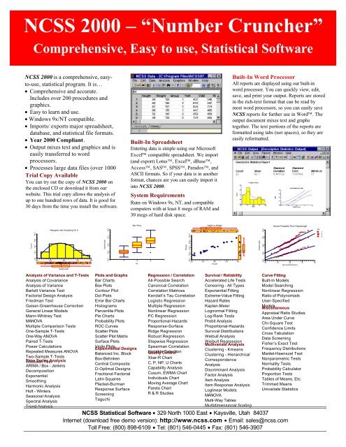
<strong>NCSS</strong> <strong>2000</strong> <strong>–</strong> <strong>“Number</strong> <strong>Cruncher”</strong><br />
<strong>NCSS</strong> <strong>2000</strong> is a comprehensive, easyto-use,<br />
statistical program. It is…<br />
• Comprehensive and accurate.<br />
Includes over 200 procedures and<br />
graphics.<br />
• Easy to learn and use.<br />
• Windows 9x/NT compatible.<br />
• Imports/ exports major spreadsheet,<br />
database, and statistical file formats.<br />
• Year <strong>2000</strong> Compliant.<br />
• Output mixes text and graphics and is<br />
easily transferred to word<br />
processors.<br />
• Processes large data files (over 1000<br />
Trial variables Copy and Available 200,000 rows).<br />
You can try out the copy of <strong>NCSS</strong> <strong>2000</strong> on<br />
the enclosed CD or download it from our<br />
website. This trial copy allows the analysis of<br />
up to one hundred rows of data. It is good for<br />
30 days from the time you install the software.<br />
Count<br />
0.0 15.0 30.0 45.0 60.0<br />
Comprehensive, Easy to use, Statistical Software<br />
Histogram with Everything On It<br />
40.0 50.0 60.0 70.0 80.0<br />
SepalLength<br />
Analysis of Variance and T-Tests<br />
Analysis of Covariance<br />
Analysis of Variance<br />
Barlett Variance Test<br />
Factorial Design Analysis<br />
Friedman Test<br />
Geiser-Greenhouse Correction<br />
General Linear Models<br />
Mann-Whitney Test<br />
MANOVA<br />
Multiple Comparison Tests<br />
One-Sample T-Tests<br />
One-Way ANOVA<br />
Paired T-Tests<br />
Power Calculations<br />
Repeated Measures ANOVA<br />
Two-Sample T-Tests<br />
Wilcoxon Time Series Test Analysis<br />
ARIMA / Box - Jenkins<br />
Decomposition<br />
Exponential<br />
Smoothing<br />
Harmonic Analysis<br />
Holt - Winters<br />
Seasonal Analysis<br />
Spectral Analysis<br />
Trend Analysis<br />
SepalLength<br />
40.0 50.0 60.0 70.0 80.0<br />
Built-In Spreadsheet<br />
Entering data is simple using our Microsoft<br />
Excel compatible spreadsheet. We import<br />
(and export) Lotus, Excel, dBase,<br />
Access, SAS, SPSS, Paradox, and<br />
ASCII formats. So if your data is in another<br />
format, chances are you can easily import it<br />
into <strong>NCSS</strong> <strong>2000</strong>.<br />
System Requirements<br />
Runs on Windows 9x, NT, and compatible<br />
computers with at least 8 megs of RAM and<br />
30 megs of hard disk space.<br />
Box Plots<br />
1 2<br />
Iris<br />
3<br />
Plots and Graphs<br />
Bar Charts<br />
Box Plots<br />
Contour Plot<br />
Dot Plots<br />
Error Bar Charts<br />
Histograms<br />
Percentile Plots<br />
Pie Charts<br />
Probability Plots<br />
ROC Curves<br />
Scatter Plots<br />
Scatter Plot Matrix<br />
Surface Plots<br />
Violin<br />
Experimental<br />
Plots<br />
Designs<br />
Balanced Inc. Block<br />
Box-Behnken<br />
Central Composite<br />
D-Optimal Designs<br />
Fractional Factorial<br />
Latin Squares<br />
Placket-Burman<br />
Response Surface<br />
Screening<br />
Taguchi<br />
Weight<br />
50.0 100.0 150.0 200.0 250.0<br />
Regression / Correlation<br />
All-Possible Search<br />
Canonical Correlation<br />
Correlation Matrices<br />
Kendall’s Tau Correlation<br />
Logistic Regression<br />
Multiple Regression<br />
Nonlinear Regression<br />
PC Regression<br />
Proportional-Hazards<br />
Response-Surface<br />
Ridge Regression<br />
Robust Regression<br />
Stepwise Regression<br />
Spearman Correlation<br />
Variable Quality Control Selection<br />
Xbar-R Chart<br />
C, P, NP, U Charts<br />
Capability Analysis<br />
Cusum, EWMA Chart<br />
Individuals Chart<br />
Moving Average Chart<br />
Pareto Chart<br />
R & R Studies<br />
Height vs Weight<br />
50.0 57.5 65.0<br />
Height<br />
72.5 80.0<br />
Survival / Reliability<br />
Accelerated Life Tests<br />
Censoring - All Types<br />
Exponential Fitting<br />
Extreme-Value Fitting<br />
Hazard Rates<br />
Kaplan-Meier<br />
Lognormal Fitting<br />
Log-Rank Tests<br />
Probit Analysis<br />
Proportional-Hazards<br />
Survival Distributions<br />
Weibull Analysis<br />
Weibull Regression<br />
Multivariate Analysis<br />
Clustering - Kmeans<br />
Clustering - Hierarchical<br />
Correspondence<br />
Analysis<br />
Discriminant Analysis<br />
Factor Analysis<br />
Item Analysis<br />
Item Response Analysis<br />
Loglinear Models<br />
MANOVA<br />
Multi-Way Tables<br />
Multidimensional Scaling<br />
Principal Components<br />
Built-In Word Processor<br />
All reports are displayed using our built-in<br />
word processor. You can quickly view, edit,<br />
save, and print your output. Reports are stored<br />
in the rich-text format that can be read by<br />
most word processors, so you can easily save<br />
<strong>NCSS</strong> reports for further use in Word. The<br />
output document mixes text and graphs<br />
together. The text portions of the reports are<br />
formatted using tabs (not spaces), so they are<br />
easily reformatted.<br />
SepalLength<br />
40.0 50.0 60.0 70.0 80.0<br />
Normal Probability Plot of SepalLength<br />
-3.0 -1.5 0.0<br />
Normal Distribution<br />
1.5 3.0<br />
Curve Fitting<br />
Built-In Models<br />
Model Searching<br />
Nonlinear Regression<br />
Ratio of Polynomials<br />
User-Specified<br />
Models<br />
Miscellaneous<br />
Appraisal Ratio Studies<br />
Area Under Curve<br />
Chi-Square Test<br />
Confidence Limits<br />
Cross Tabulation<br />
Data Screening<br />
Fisher’s Exact Test<br />
Frequency Distributions<br />
Mantel-Haenszel Test<br />
Nonparametric Tests<br />
Normality Tests<br />
Probability Calculator<br />
Proportion Tests<br />
Tables of Means, Etc.<br />
Trimmed Means<br />
Univariate Statistics<br />
<strong>NCSS</strong> Statistical Software • 329 North 1000 East • Kaysville, Utah 84037<br />
Internet (download free demo version): http://www.ncss.com • Email: sales@ncss.com<br />
Toll Free: (800) 898-6109 • Tel: (801) 546-0445 • Fax: (801) 546-3907<br />
Iris<br />
1<br />
3<br />
2
<strong>NCSS</strong> provides and complete set of statistical charts and graphs. You control the labels, lines, and<br />
colors of the graphs. The graphs may be copied to your favorite word processor or graphics editing<br />
package.<br />
SepalLength<br />
40.0 50.0 60.0 70.0 80.0<br />
SepalWidth<br />
15.0 22.5 30.0 37.5 45.0<br />
SepalLength<br />
40.0 50.0 60.0 70.0 80.0<br />
Amount<br />
0.0 20.0 40.0 60.0 80.0<br />
Box Plots<br />
1 2<br />
Iris<br />
3<br />
Grid Plot of PetalLength<br />
40.0 50.0 60.0<br />
SepalLength<br />
70.0 80.0<br />
Normal Probability Plot of SepalLength<br />
PetalLength<br />
A 3.5<br />
B 10.5<br />
C 17.5<br />
D 24.5<br />
E 31.5<br />
F 38.5<br />
G 45.5<br />
H 52.5<br />
I 59.5<br />
J 66.5<br />
-3.0 -1.5 0.0<br />
Normal Distribution<br />
1.5 3.0<br />
SepalLength<br />
Violin Plots at 30% Data<br />
SepalWidth<br />
Variables<br />
PetalLength<br />
PetalWidth<br />
• Box plot<br />
• Chi-square probability plot<br />
• Density trace<br />
• Dot plot<br />
• Exponential probability plot<br />
• Frequency polygon<br />
• Gamma probability plot<br />
Charts and Graphs<br />
Test2<br />
0.0 25.0 50.0 75.0 100.0<br />
Count<br />
0.0 15.0 30.0 45.0 60.0<br />
FailTime<br />
Weight<br />
50.0 100.0 150.0 200.0 250.0<br />
Contour Plot of Test3<br />
Sample Plots<br />
30.0 47.5 65.0<br />
Test1<br />
82.5 100.0<br />
Density Trace at 20% Data Range<br />
40.0 50.0 60.0 70.0 80.0<br />
1000<br />
100<br />
10<br />
0.10<br />
SepalLength<br />
Weibull Probability Plot of FailTime<br />
0.20<br />
0.80<br />
0.70<br />
0.60<br />
0.50<br />
0.40<br />
0.30<br />
Weibull Distribution<br />
Height vs Weight<br />
Test3<br />
40.0<br />
50.0<br />
60.0<br />
70.0<br />
80.0<br />
90.0<br />
50.0 57.5 65.0<br />
Height<br />
72.5 80.0<br />
0.90<br />
Count<br />
0.0 15.0 30.0 45.0 60.0<br />
Weight<br />
50.0 100.0 150.0 200.0 250.0<br />
Weight<br />
50.0 100.0 150.0 200.0 250.0<br />
• Grid plot<br />
• Half normal probability plot<br />
• Histogram<br />
• Normal probability plot<br />
• Percentile plot<br />
• Scatter plot<br />
• Scatter plot matrix<br />
SepalLength<br />
40.0 50.0 60.0 70.0 80.0<br />
Dot Plots<br />
1 2<br />
Iris<br />
3<br />
Histogram with Everything On It<br />
40.0 50.0 60.0 70.0 80.0<br />
SepalLength<br />
Height vs Weight<br />
50.0 57.5 65.0<br />
Height<br />
72.5 80.0<br />
Height vs Weight<br />
50.0 57.5 65.0<br />
Height<br />
72.5 80.0<br />
• Sunflower plot<br />
• Uniform probability plot<br />
• Violin plot<br />
• Weibull probability plot
Descriptive Statistics and Cross Tabulation<br />
Several procedures are available for tabulating and summarizing your data. The frequency table<br />
procedure provides tabulation of single variables. The cross tabulation procedure provides tabulation<br />
of two variables into two-way tables. The descriptive tables procedure computes summary statistics<br />
(means, median, standard deviations, etc.) according to up to eight breakdown variables. All of<br />
these procedures provide numeric and graphic reports. A specialized appraisal ratio module provides<br />
reports for mass appraisal.<br />
Frequency Table Report<br />
Row Percentages Section<br />
Values<br />
Variables 0 0.5 1 2 3 Total<br />
Garage Size 4.7 0.0 65.3 28.7 1.3 100.0<br />
Fireplaces 26.0 0.0 52.0 22.0 0.0 100.0<br />
Brick Ratio 34.0 31.3 34.7 0.0 0.0 100.0<br />
Total 21.6 10.4 50.7 16.9 0.4 100.0<br />
Column Percentages Section<br />
Values<br />
Variables 0 0.5 1 2 3 Total<br />
Garage Size 7.2 0.0 43.0 56.6 100.0 33.3<br />
Fireplaces 40.2 0.0 34.2 43.4 0.0 33.3<br />
Brick Ratio 52.6 100.0 22.8 0.0 0.0 33.3<br />
Total 100.0 100.0 100.0 100.0 100.0 100.0<br />
Row Pct<br />
80.0<br />
55.0<br />
30.0<br />
5.0<br />
-20.0<br />
Row Pct of Values by Variables<br />
0 0.5 1<br />
Values<br />
2 3<br />
• Cross Tabulation<br />
• Armitage test for trend<br />
• Break Variables (up to five)<br />
• Chi-square test<br />
• Contingency analysis<br />
• Continuous variables allowed<br />
• Cramer’s V<br />
• Expected values<br />
• Fisher’s exact test<br />
• Gamma<br />
• Kendall’s tau - B & C<br />
• Lambda A & B<br />
• McNemar Test<br />
• Percentages<br />
• Phi coefficient<br />
• Text variables allowed<br />
• Tschuprow’s T<br />
• Value labels<br />
Variables<br />
Garage Size<br />
Fireplaces<br />
Brick Ratio<br />
Column Pct<br />
120.0<br />
85.0<br />
50.0<br />
15.0<br />
-20.0<br />
• Descriptive Statistics<br />
• Average absolute deviation<br />
• Coef. of dispersion - COD<br />
• Coefficient of variation<br />
• Confidence limits<br />
• Density trace<br />
• Fisher’s g1 and g2<br />
• Geometric mean<br />
• Harmonic mean<br />
• Histogram<br />
• Kurtosis measures<br />
• Means, medians, modes<br />
• Mininmum and maximum<br />
• Normal probability plot<br />
• Normality tests<br />
• Percentiles<br />
• Price-related diff. - PRD<br />
• Skewness measures<br />
• Standard deviation / error<br />
• Stem-leaf plot<br />
• Trimmed mean<br />
Column Pct of Values by Variables<br />
0 0.5 1<br />
Values<br />
2 3<br />
Variables<br />
Garage Size<br />
Fireplaces<br />
Brick Ratio<br />
• Descriptive Tables<br />
• Numeric break variables<br />
• One-way and Two-way tables<br />
• Plots of tabulated statistics<br />
• Tables of medians, means,<br />
standard deviations, counts,<br />
COV’s, and COD’s<br />
• Text break variables<br />
• Value labels<br />
• Frequency Tables<br />
• Chi-square test<br />
• Counts<br />
• Cumulative statistics<br />
• Frequency distribution<br />
• Multinomial test<br />
• Percents
Curve fitting refers to nonlinear-regression techniques for fitting curved lines to X-Y data. You can<br />
select a standard model from the large list of precoded models or you can enter your own. If you do<br />
not have a specific model in mind, the program can search through hundreds of possible models<br />
looking for the one that best fits your data. The program will fit models with up to four independent<br />
variables.<br />
Model Estimation Section<br />
Parameter Parameter Asymptotic Lower Upper<br />
Name Estimate Standard Error 95% C.L. 95% C.L.<br />
A 0.3901402 5.033759E-03 0.3799816 0.4002987<br />
B 0.101633 1.336168E-02 7.466801E-02 0.1285979<br />
Dependent Y<br />
Independent X<br />
Model Y = A+(0.49-A)*EXP(-B*(X-8))<br />
R-Squared 0.873375<br />
Iterations 13<br />
Estimated Model<br />
(.3901402)+(0.49-(.3901402))*EXP(-(.101633)*((X)-8))<br />
Predicted Values and Residuals Section<br />
Row Predicted Lower 95.0% Upper 95.0%<br />
No. X Y Value Value Value Residual<br />
1 8 0.49 0.49 0.4679772 0.5120228 0<br />
2 8 0.49 0.49 0.4679772 0.5120228 0<br />
3 10 0.48 0.4716319 0.4494232 0.4938406 0.0083681<br />
4 10 0.47 0.4716319 0.4494232 0.4938406 -0.0016319<br />
5 10 0.48 0.4716319 0.4494232 0.4938406 0.0083681<br />
Y<br />
0.4 0.4 0.5 0.5 0.6<br />
Plot of Y = A+(0.49-A)*EXP(-B*(X-8))<br />
5.0 15.0 25.0<br />
X<br />
35.0 45.0<br />
• Bleasdale-Nelder Model<br />
• Double-Exponential Model<br />
• Exponential Model<br />
• Farazdaghi Model<br />
• Gompertz Models<br />
• Goodness of Fit Measures<br />
• Holliday Model<br />
• Logistic Model<br />
• Lognormal Model<br />
Curve Fitting<br />
Y<br />
10.0 25.0 40.0 55.0 70.0<br />
• Marquart algorithm<br />
• Monomolecular Model<br />
• Morgan-Mercer Model<br />
• Nonlinear Regression<br />
• Normal Model<br />
• Piecewise-Polynomials<br />
• Probability Plots<br />
• Ratio of Polynomials<br />
• Reciprocal Model<br />
Y = PolyRatio(X, 3, 4)<br />
0.0 25.0 50.0<br />
X<br />
75.0 100.0<br />
• Richards Model<br />
• Scatter-Plot Matrix<br />
• Search Routines<br />
• Sum of Functions Regression<br />
• Transformation Bias<br />
Correction<br />
• User-Supplied Models<br />
• Weibull Model
Regression analysis refers to a group of techniques for studying the relationships among two or<br />
more variables. <strong>NCSS</strong> makes it easy to run either a simple linear regression analysis or a complex<br />
multiple regression analysis. You can perform a regression analysis with modern graphical and<br />
numeric residual analysis. Major options include multiple regression, stepwise regression, correlation<br />
matrix, residual analysis, robust regression, all-possible regressions, response surface regression,<br />
proportional hazards regression, ridge regression, and logistic regression.<br />
Regression Equation Section<br />
Multiple Regression Report<br />
Independent Regression Standard T-Value Prob Decision Power<br />
Variable Coefficient Error (Ho: B=0) Level (5%) (5%)<br />
Intercept 85.24039 23.69514 3.5974 .005772 Reject Ho .891498<br />
Test1 -1.933571 1.029096 -1.8789 .092969 Accept Ho .389629<br />
Test2 -1.659881 .872896 -1.9016 .089661 Accept Ho .397357<br />
Test3 .1049543 .219902 .4773 .644541 Accept Ho .071290<br />
R-Squared .399068<br />
Normality Tests Section<br />
Assumption Value Probability Decision(5%)<br />
Skewness 2.0329 .042064 Rejected<br />
Kurtosis 1.5798 .114144 Accepted<br />
Omnibus 6.6285 .036361 Rejected<br />
Count<br />
0.0 2.0 4.0 6.0 8.0<br />
Histogram<br />
-15.0 -5.0 5.0 15.0 25.0<br />
• All-possible regressions<br />
• Alpha level is flexible<br />
• Beta coefficients<br />
• Biweight regression<br />
• Coefficient of variation<br />
• Condition number<br />
• Confidence limits<br />
• Cook’s D<br />
• Correlations<br />
• CovRatio<br />
• Cp Statistic<br />
• DFBetas<br />
• Dffits<br />
• Durbin Watson statistic<br />
• Eigenvalues<br />
• Eigenvectors<br />
• F-ratios<br />
• Hat diagonal<br />
• Inverse diagonal<br />
• LAV regression<br />
Residuals of IQ<br />
Regression Analysis<br />
Residuals of IQ<br />
-15.0 -5.0 5.0 15.0 25.0<br />
• Logistic regression<br />
• Mean squares<br />
• Multiple regression<br />
• Multiple regression<br />
• Normal probability plot<br />
• Normality tests of residuals<br />
• Partial correlation<br />
• Pearson’s correlation<br />
• Power calculations<br />
• Predicted values<br />
• Prediction limits<br />
• Predicts new observations<br />
• Press statistic<br />
• P.C. Regression<br />
• Proportional-Hazards<br />
• R-bar squared<br />
• R-squared<br />
• Regression coefficient<br />
• Residual analysis and plots<br />
• Response surface analysis<br />
Normal Probability Plot of Residuals of IQ<br />
-2.0 -1.0 0.0<br />
Normal Distribution<br />
1.0 2.0<br />
• Ridge Regression<br />
• Robust regression<br />
• Rstudent<br />
• Serial correlation plot<br />
• Simple linear regression<br />
• Spearman’s rank correlation<br />
• Standard error of beta<br />
• Standardized coefficient<br />
• Stepwise regression<br />
• Sum of squares<br />
• T-test for beta=0<br />
• Through the origin<br />
• Tolerance level<br />
• Variable selection<br />
• Variance inflation factor<br />
• Weighted regression
The t-test procedures test the difference between two averages. The two sample t-test is used when<br />
the means come from two independent samples. The paired t-test is used when the observations<br />
are obtained in pairs. The one sample t-test is used to compare a single mean with a target value.<br />
<strong>NCSS</strong> offers a comprehensive t-test analysis. It automatically checks all model assumptions,<br />
performs analogous nonparametric tests, displays appropriate plots, and computes confidence limits.<br />
Two-Sample T-Test<br />
Descriptive Statistics Section<br />
Standard Standard 95% LCL 95% UCL<br />
Variable Count Mean Deviation Error of Mean of Mean<br />
YldA 13 549.3846 168.7629 46.80641 447.4022 651.367<br />
YldB 16 557.5 104.6219 26.15546 501.7509 613.249<br />
Confidence-Limits of Difference Section<br />
Variance Mean Standard Standard 95% LCL 95% UCL<br />
Assumption DF Difference Deviation Error of Mean of Mean<br />
Equal 27 -8.115385 136.891 51.11428 -112.9932 96.76247<br />
Unequal 19.1690 -8.115385 198.5615 53.61855 -120.2734 104.0426<br />
Equal-Variance T-Test Section<br />
Alternative Prob Decision Power Power<br />
Hypothesis T-Value Level (5%) (Alpha=.05) (Alpha=.01)<br />
(YldA)-(YldB)0 -0.1588 0.875032 Accept Ho 0.052693 0.010837<br />
(YldA)-(YldB)0 -0.1588 0.562484 Accept Ho 0.035954 0.006616<br />
Tests of Assumptions Section<br />
Assumption Value Probability Decision(5%)<br />
Skewness Normality (YldA) 0.2691 0.787854 Cannot reject normality<br />
Kurtosis Normality (YldA) 0.3081 0.758028 Cannot reject normality<br />
Omnibus Normality (YldA) 0.1673 0.919743 Cannot reject normality<br />
Variance-Ratio Equal-Variance Test 2.6020 0.092546 Cannot reject equal variances<br />
Modified-Levene Equal-Variance Test 13.9235 0.002234 Reject equal variances<br />
Amount<br />
200.0 400.0 600.0 800.0 1000.0<br />
Box Plots<br />
YldA YldB<br />
Variables<br />
• Aspin-Welch unequal-variance<br />
test<br />
• Box plots<br />
• Confidence limits<br />
• Descriptive statistics<br />
• Kolmogorov-Smirnov test<br />
• Levene equal-variance test<br />
T-Tests<br />
YldB<br />
300.0 425.0 550.0 675.0 800.0<br />
• Mann-Whitney U test<br />
• Normal probability plots<br />
• Normality tests<br />
• One and two tailed tests<br />
• One sample t-test<br />
• Pair comparisons t-test<br />
Normal Probability Plot of YldB<br />
-2.0 -1.0 0.0<br />
Normal Distribution<br />
1.0 2.0<br />
• Power calculations<br />
• Probability levels<br />
• Quantile test<br />
• Two sample t-test<br />
• Unequal variance case<br />
• Wilcoxon rank sum test
Analysis of variance is the statistical technique for testing differences among group means. <strong>NCSS</strong><br />
contains several analysis of variance procedures, including general linear models (GLM), one-way<br />
analysis of variance, unweighted means analysis of variance, and MANOVA. You can perform a<br />
simple one-way analysis of variance, a complex repeated-measures analysis of variance, a factorial<br />
analysis of variance, an analysis of covariance, and a host of multiple-comparison tests. All<br />
procedures work with balanced and unbalanced experimental designs.<br />
Analysis of Variance Table<br />
Source Sum of Mean Prob Power<br />
Term DF Squares Square F-Ratio Level (Alpha=0.05)<br />
A (Treatment) 3 486.7488 165.5833 .61 .555761 .089834<br />
B(A) 15 4064.833 270.9889<br />
C (Time) 1 277.7778 277.7778 50.51 .000004* .995231<br />
AC 3 352.0833 117.3611 21.34 .000041* .968851<br />
BC(A) 15 82.5 5.5<br />
Tukey's HSD Multiple-Comparison Test<br />
Term A: Exercise<br />
Alpha=0.050 Error Term=B(A) DF=15 MSE=270.9889 Critical Value=4.895637<br />
Different<br />
Group Count Mean From Groups<br />
1 3 210.6667<br />
4 3 211.3333<br />
3 3 238<br />
2 3 257.6667<br />
Response<br />
100.0 150.0 200.0 250.0 300.0<br />
Means of Response<br />
1 2 3 4<br />
Treatment<br />
• Analysis of covariance<br />
• ANOVA table<br />
• Area Under Curve<br />
• Assumptions testing<br />
• Automatic F-ratios<br />
• Bonferroni tests<br />
• Box plots<br />
• Box’s M test<br />
• Comparisons<br />
• Contrasts<br />
• Covariance analysis<br />
• Duncans test<br />
• Expected mean squares<br />
• F-ratios<br />
• Factorial designs<br />
• Fishers LSD test<br />
• Fixed terms<br />
• Fractional factorial designs<br />
• Geisser-Greenhouse<br />
• GLM solution<br />
Analysis of Variance<br />
Response<br />
• Hotelling’s trace<br />
• Huynh-Feldt Correction<br />
• Interation plots<br />
• Kruskal Wallis z tests<br />
• Latin square designs<br />
• Least-squares means<br />
• Levene Variance test<br />
• MANOVA (with up to 10<br />
factors)<br />
• Mauchley’s Test<br />
• Mean Squares<br />
• Means plots<br />
• Multiple comparisons of<br />
factors<br />
• Multiple comparisons of<br />
interactions<br />
• Nested terms<br />
• Newman-Keuls test<br />
• Normality tests<br />
• Pillai’s Trace<br />
100.0 150.0 200.0 250.0 300.0<br />
Means of Response<br />
1 2<br />
Blocks<br />
3<br />
Treatment<br />
1<br />
2<br />
3<br />
4<br />
• Planned comparisions<br />
• Post-hoc tests<br />
• Power calculations<br />
• Random terms<br />
• Randomized complete block<br />
• Repeated measures<br />
• R and R Study<br />
• Roy’s Root<br />
• Scheffe’s test<br />
• Split-plot designs<br />
• Tukey-Kramer HSD tests<br />
• Unbalanced data<br />
• Wilks’ Lambda
The repeated measures procedure performs an analysis of variance on within-subject designs using<br />
the general linear models approach. The experimental design may include up to three betweensubject<br />
factors as well as three within-subject factors. Box’s M test and Mauchley’s test of the<br />
assumptions about the within-subject covariance matrices are provided. Geisser-Greenhouse, Box,<br />
and Huynh-Feldt corrected probability levels on the within-subject F tests are given along with the<br />
associated test power.<br />
Analysis of Variance Table<br />
Source Sum of Mean Prob Power<br />
Term DF Squares Square F-Ratio Level (Alpha=0.05)<br />
A: Exercise 2 427.4445 213.7222 0.61 0.555040 0.076179<br />
B(A): Subject 15 5234.556 348.9704<br />
C: Time 2 547.4445 273.7222 36.92 0.000000* 0.999974<br />
AC 4 191.4444 47.86111 6.45 0.000716* 0.874052<br />
BC(A) 30 222.4444 7.414815<br />
Probability Levels for F-Tests with Geisser-Greenhouse Adjustments<br />
Geisser Huynh<br />
Greenhouse Box Feldt<br />
Regular Epsilon Epsilon Epsilon<br />
Source Prob Prob Prob Prob<br />
Term DF F-Ratio Level Level Level Level<br />
A: Exercise 2 0.61 0.555040<br />
B(A): Subject 15<br />
C: Time 2 36.92 0.000000* 0.000021* 0.000000* 0.000000*<br />
AC 4 6.45 0.000716* 0.009496* 0.000755* 0.000716*<br />
BC(A) 30<br />
Power Values for F-Tests with Geisser-Greenhouse Adjustments<br />
Geisser Huynh<br />
Greenhouse Box Feldt<br />
Regular Epsilon Epsilon Epsilon<br />
Source Power Power Power Power<br />
Term DF F-Ratio (Alpha=0.05) (Alpha=0.05) (Alpha=0.05) (Alpha=0.05)<br />
A: Exercise 2 0.61 0.076179<br />
B(A): Subject 15<br />
C: Time 2 36.92 0.999974 0.889537 0.999966 0.999974<br />
AC 4 6.45 0.874052 0.371111 0.867399 0.874052<br />
BC(A) 30<br />
HeartRate<br />
90.00<br />
78.75<br />
67.50<br />
56.25<br />
45.00<br />
Means of HeartRate<br />
0 - None 1 - Week<br />
Exercise<br />
2 - Dail<br />
• Analysis of variance<br />
• Box’s M test<br />
• Circularity test<br />
• Compound symmetry test<br />
• Contrasts<br />
• Covariance matrix tests<br />
• Epsilon values<br />
• F ratios<br />
Repeated Measures ANOVA<br />
Time<br />
0<br />
10<br />
20<br />
HeartRate<br />
90.00<br />
78.75<br />
67.50<br />
56.25<br />
45.00<br />
• Fixed or random factors<br />
• Geisser-Greenhouse<br />
• Huynh-Feldt correction<br />
• Mauchley’s test<br />
• Means plots<br />
• Multiple comparisons<br />
• Planned comparisons<br />
• Power values<br />
HeartRate vs Time by Subject<br />
0 10<br />
Time<br />
20<br />
• Probability levels<br />
• Randomized block designs<br />
• Repeated measures<br />
• Subject plots<br />
• Within-subject designs
These programs can generate 2 k factorial designs, B.I.B. designs, d-optimal designs, fractional<br />
factorial designs, Latin square designs, screening designs, Taguchi designs, and response surface<br />
designs. <strong>NCSS</strong> also provides for the analysis of these designs using either the general purpose<br />
ANOVA and regression procedures or specialized procedures for designs with factors at only two<br />
levels.<br />
Means and Effects Section<br />
Term Term Estimated Standard<br />
No. Symbol Mean - Mean + Effect Error<br />
0 Grand Mean 64.25 0.71<br />
1 A (Temp) 52.75 75.75 23.00 1.41<br />
2 B (Concentration) 66.75 61.75 -5.00 1.41<br />
3 AB 63.50 65.00 1.50 1.41<br />
4 C (Catalyst) 63.50 65.00 1.50 1.41<br />
5 AC 59.25 69.25 10.00 1.41<br />
6 BC 64.25 64.25 0.00 1.41<br />
7 ABC 64.00 64.50 0.50 1.41<br />
Analysis of Variance Section<br />
Term Term Mean Prob Statistically<br />
No. Symbol DF Square F-Ratio Level Significant<br />
1 A (Temp) 1 2116.0000 264.50 0.000000 Yes<br />
2 B (Concentration) 1 100.0000 12.50 0.007670 Yes<br />
3 AB 1 9.0000 1.13 0.319813 No<br />
4 C (Catalyst) 1 9.0000 1.13 0.319813 No<br />
5 AC 1 400.0000 50.00 0.000105 Yes<br />
6 BC 1 0.0000 0.00 1.000000 No<br />
7 ABC 1 1.0000 0.13 0.732810 No<br />
Error 8 8.0000<br />
Total 15 2699.0000<br />
Effects<br />
-10.0 -1.3 7.5 16.3 25.0<br />
Normal Probability Plot of Effects<br />
-1.5 -0.8 0.0<br />
Normal Distribution<br />
0.8 1.5<br />
• Aliasing reports<br />
• Analysis of variance tables<br />
• Automatic design detection<br />
• Balanced incomplete block<br />
• Block confounding<br />
• Blocking<br />
• Box-Behnken designs<br />
• Box-Hunter-Hunter designs<br />
• Central composite designs<br />
• Contour plots<br />
Design of Experiments<br />
Temp<br />
-1.5 -0.8 0.0 0.8 1.5<br />
• D-optimal designs<br />
• Effect estimation<br />
• Fractional factorials<br />
• Latin Squares<br />
• Factorial designs<br />
• Means Plots<br />
• Placket-burman designs<br />
• Probability plots of residuals<br />
and effects<br />
• Repeated Measures designs<br />
Contour Plot of Odor<br />
-2 -1 0<br />
Ratio<br />
1 2<br />
Odor<br />
-40.0<br />
-20.0<br />
0.0<br />
20.0<br />
40.0<br />
60.0<br />
80.0<br />
100.0<br />
120.0<br />
140.0<br />
• Residual analysis<br />
• Response-surface designs<br />
• Screening designs (up to 31<br />
Factors)<br />
• Taguchi designs
Survival analysis includes several techniques to study data in which the response variable is elapsed<br />
time. Procedures include survival distribution analysis (including the Kaplan-Meier survival<br />
distribution estimate), log rank tests, and proportional hazards regression.<br />
S(t) Exponential<br />
Kaplan-Meier Product-Limit Survival Distribution<br />
Sample Survivorship Std Error Hazard Fn Std Error<br />
Rank Size Time S(t) of S(t) H(t)=-Log(S(t)) of H(t)<br />
1 19 3.0 .947368 .051228 .054067 .238910<br />
2 18 3.0+<br />
3 17 4.0 .891641 .072440 .114692 .301855<br />
4 16 6.0 .835913 .086738 .179230 .352326<br />
5 15 8.0 .780186 .097223 .248223 .399657<br />
6 14 8.0 .724458 .105043 .322331 .447373<br />
7 13 8.0+<br />
8 12 10.0 .664087 .112306 .409343 .504634<br />
9 11 12.0 .603715 .117205 .504653 .567076<br />
10 10 13.0+<br />
11 9 16.0 .536636 .121875 .622436 .650547<br />
12 8 17.0 .469556 .123732 .755967 .749122<br />
13 7 21.0+<br />
14 6 26.0+<br />
15 5 30.0 .375645 .129821 .979111 .959169<br />
16 4 33.0 .281734 .126865 1.266793 1.264245<br />
17 3 35.0+<br />
18 2 44.0+<br />
19 1 45.0+<br />
0.000 0.250 0.500 0.750 1.000<br />
S(t) Exponential Plot<br />
0.0 12.5 25.0<br />
TIME3<br />
37.5 50.0<br />
• Accelerated life testing<br />
• Beta distribution<br />
• Censoring <strong>–</strong> All Types<br />
• Cox’s regression<br />
• Cox-Mantel test<br />
• Exponential distribution<br />
• Exponential regression<br />
• Extreme Value distribution<br />
• Extreme Value regression<br />
• Gamma distribution<br />
• Gehan’s Wilcoxon test<br />
• Goodness of fit<br />
Survival Analysis<br />
Hazard Function<br />
0.000 0.350 0.700 1.050 1.400<br />
• Hazard rate plots<br />
• Hazard functions & plots<br />
• Kaplan-Meier product limit<br />
• Least squares estimates<br />
• Log-logistic distribution<br />
• Log-logistic regression<br />
• Log rank test<br />
• Lognormal distribution<br />
• Lognormal regression<br />
• Maximum likelihood<br />
• Peto / Wilcoxon test<br />
• Probit Analysis<br />
Hazard Function Plot<br />
0.0 12.5 25.0<br />
TIME3<br />
37.5 50.0<br />
• Proportional hazards<br />
regression<br />
• Rayleigh distribution<br />
• Reliability statistics<br />
• Stress variables<br />
• Survival functions & plots<br />
• Survival percentiles<br />
• Variable selection options<br />
• Weibull distribution<br />
• Weibull regression
The reliability procedure estimates the parameters of the exponential, extreme value, logistic, loglogistic,<br />
lognormal, normal, and Weibull probability distributions by maximum likelihood and least<br />
squares. It can fit complete, right censored, left censored, interval censored (readout), and grouped<br />
data values. It also computes the nonparametric Kaplan-Meier and Nelson-Aalen estimates of<br />
reliability and associated hazard rates.<br />
Another module fits the regression relationship between time-to-failure and one or more<br />
independent variables. The distribution of the residuals (errors) can follow the exponential, extreme<br />
value, logistic, log-logistic, lognormal, lognormal10, normal, or Weibull distributions. The data may<br />
include failed, left censored, right censored, and interval observations. This type of data often arises<br />
in the area of accelerated life testing.<br />
Weibull Parameter Estimation Section<br />
Probability Maximum MLE MLE MLE<br />
Plot Likelihood Standard 95% Lower 95% Upper<br />
Parameter Estimate Estimate Error Conf. Limit Conf. Limit<br />
Shape 1.26829 1.511543 0.4128574 0.8849655 2.581753<br />
Scale 279.7478 238.3481 57.21616 148.8944 381.5444<br />
Log Likelihood -80.05649<br />
Reliability Section<br />
Prob Prob Max Like 95% Lower 95% Upper<br />
Failure Estimate of Estimate of Conf. Limit of Conf. Limit of<br />
Time Survival Survival Survival Survival<br />
40.0 0.9186 0.9349 0.8065 0.9791<br />
80.0 0.8151 0.8253 0.6728 0.9112<br />
120.0 0.7105 0.7016 0.5312 0.8199<br />
160.0 0.6112 0.5784 0.3775 0.7352<br />
Percentile Section<br />
Prob Prob Max Like 95% Lower 95% Upper<br />
Failure Estimate of Estimate of Conf. Limit of Conf. Limit of<br />
Time Failure Failure Failure Failure<br />
Percentage Time Time Time Time<br />
25.0000 104.7 104.5 69.7 156.8<br />
50.0000 209.5 187.0 124.7 280.5<br />
75.0000 361.9 295.8 170.9 512.1<br />
95.0000 664.5 492.6 227.8 1065.0<br />
Hazard Rate<br />
0.010<br />
0.008<br />
0.005<br />
0.003<br />
Weibull Hazard Rate Plot<br />
0.000<br />
0.0 50.0 100.0<br />
Time<br />
150.0 200.0<br />
• Accelerated life testing<br />
• Arrhenius transformation<br />
• Beta distribution<br />
• Censoring <strong>–</strong> All Types<br />
• Confidence Limits<br />
• Cox-Snell Residuals<br />
• Distribution selection<br />
• Exponential distribution<br />
• Exponential regression<br />
• Extreme-value distribution<br />
• Extreme-value regression<br />
• Failure time percentiles<br />
Reliability Analysis<br />
Ln(Time)<br />
5.50<br />
4.75<br />
4.00<br />
3.25<br />
• Gamma distribution<br />
• Goodness of fit<br />
• Hazard rate plots<br />
• Hazard functions & plots<br />
• Information Matrix<br />
• Kaplan-Meier product limit<br />
• Least squares estimates<br />
• Log-logistic distribution<br />
• Log-logistic regression<br />
• Lognormal distribution<br />
• Lognormal regression<br />
• Maximum likelihood<br />
Weibull Probability Plot<br />
2.50<br />
-4.00 -3.13 -2.25<br />
Weibull Quantile<br />
-1.38 -0.50<br />
• Probability plots<br />
• Reliability statistics<br />
• Residual Analysis<br />
• Residual Life Report<br />
• Stress variables<br />
• Stress plots<br />
• Threshold Estimate<br />
• Weibull distribution<br />
• Weibull regression
<strong>NCSS</strong> provides a complete set of the latest variables and attribute control charts. It includes popular<br />
features such as runs tests, individuals charts, automatic outlier removal, capability analysis, usersupplied<br />
sigma, and comprehensive chart labeling. Since the quality control programs are completely<br />
integrated with the rest of the system, once you detect an out-of-control signal, you can investigate<br />
with the other procedures in <strong>NCSS</strong>.<br />
Xbar and R Charts<br />
Xbar<br />
1980.0 1988.8 1997.5 2006.3 2015.0<br />
Quality Control Charts and SPC<br />
13 22<br />
36<br />
Xbar Chart<br />
0.0 30.0 60.0<br />
Row<br />
90.0 120.0<br />
Range<br />
-10.0 7.5 25.0 42.5 60.0<br />
11<br />
Range Chart<br />
0.0 30.0 60.0<br />
Row<br />
90.0 120.0<br />
Out-of-Control List<br />
Row Mean Range Row Label Reason<br />
4 6.8 5 4 Range: 4 of 5 in zone B or beyond<br />
5 12.2 48 5 Xbar: beyond control limits<br />
6 9.8 27 6 Xbar: 2 of 3 in zone A<br />
7 5.6 4 7 Xbar: 2 of 3 in zone A<br />
Capability Analysis Section<br />
Parameter Lower Center Upper<br />
3-Sigma Limits -5.390758 6.036585 17.46393<br />
4-Sigma Limits -9.199872 6.036585 21.27304<br />
Specification Limits 1 14<br />
Specification z-Values -1.322246 2.090621<br />
Percent Outside Specification 3.252033 2.439024<br />
Capacities 0.440749 0.696874<br />
Cp Index 0.518452 0.568811 0.619112<br />
Cpk Index 0.383108 0.440749 0.498389<br />
Count = 246 Sigma = 3.809114 Alpha Level = 0.050000<br />
• Attribute charts<br />
• C chart<br />
• Capability analysis<br />
• Cp index<br />
• Cpk Index<br />
• Cusum chart<br />
• EWMA chart<br />
• Exception report<br />
• Frequency distribution<br />
• Histogram<br />
• Individuals chart<br />
• Moving average chart<br />
• Moving range chart<br />
• Normality test<br />
• NP chart<br />
• Out-of-control list<br />
• P chart<br />
• Pareto charts<br />
• Primary control limits<br />
• R and R Study<br />
• R chart<br />
• Robust chart analysis<br />
• Runs tests<br />
• S (sigma) chart<br />
• Secondary control limits<br />
• U chart<br />
• Variables charts<br />
• Xbar chart<br />
• Zone display
Multivariate analysis refers to a group of statistical techniques that analyze two or more variables at<br />
a time, including: discriminant analysis, factor analysis, cluster analysis, logistic regression,<br />
MANOVA, and principal component analysis.<br />
Factor Analysis Report<br />
Eigenvalues after Varimax Rotation<br />
Individual Cumulative<br />
No. Eigenvalue Percent Percent Scree Plot<br />
1 3.288191 54.89 54.89 |||||||||||<br />
2 2.701207 45.09 99.99 ||||||||||<br />
3 0.001207 0.02 100.00 |<br />
4 -.000099 0.00 100.00 |<br />
5 -.000121 0.00 100.00 |<br />
6 -.000295 0.00 100.00 |<br />
Factor Loadings after Varimax Rotation<br />
Variables Factor1 Factor2<br />
X1 -.019936 -.998792<br />
X2 -.967470 -.252572<br />
X3 -.994037 -.107126<br />
X4 -.478418 -.873578<br />
X5 -.594943 -.803812<br />
X6 -.883654 -.468080<br />
Score1<br />
-2.0 -0.8 0.5 1.8 3.0<br />
15<br />
17 11<br />
23<br />
12<br />
14<br />
19<br />
521<br />
Factor Scores<br />
18<br />
3<br />
1<br />
16<br />
20 27<br />
9 7<br />
4<br />
8<br />
25<br />
-2.0 -1.0 0.0<br />
Score2<br />
1.0 2.0<br />
• Discriminant Analysis<br />
• Canonical coefficient reports<br />
• Classification reports<br />
• Influential variable reports<br />
• Linear discriminant functions,<br />
scores, and coefficients<br />
• Prior probabilities<br />
• Stepwise variable selection<br />
• Cluster Algorithms<br />
• Complete Linkage<br />
• Dendrograms<br />
• Fuzzy clustering<br />
• Hierarchical<br />
• K-means algorithm<br />
• Mediod partitioning<br />
• Nearest neighbor<br />
• Regression clustering<br />
• Single Linkage<br />
Multivariate Analysis<br />
30<br />
26<br />
13<br />
2<br />
6 24<br />
28 29<br />
22<br />
10<br />
Loading1<br />
-1.0 -0.8 -0.5 -0.3 0.0<br />
• Factor and Principal<br />
Component Analysis<br />
• Bartlett’s sphericity test<br />
• Communality estimates<br />
• Correlation matrix input<br />
• Eigenvalue/vector analysis<br />
• Factor loadings and scores<br />
• Gleason-Staelin redundancy<br />
• Missing value estimation<br />
• Outlier detection<br />
• Principal axis method<br />
• Quartimax rotation<br />
• Robust estimation<br />
• Score and Loading Plots<br />
• Scree plot<br />
• T 2 analysis<br />
• Varimax rotation<br />
• Equality of Covariance<br />
• Bartlett’s variance test<br />
• Box’s M test<br />
• Cronbachs alpha<br />
• Eigenvalue analysis<br />
1<br />
4<br />
5<br />
Factor Loadings<br />
6<br />
2<br />
3<br />
-1.0 -0.8 -0.5<br />
Loading2<br />
-0.3 0.0<br />
• MANOVA<br />
• Approximate F-test<br />
• Box’s M test<br />
• Canonical analysis<br />
• Homogeneity of variance test<br />
• Hotelling’s T 2<br />
• Lawley-Hotelling trace<br />
• Pillai’s trace<br />
• Roy’s largest root<br />
• Wilks’ lambda<br />
• Logistic Regression<br />
• Beta estimates<br />
• Chi-square tests<br />
• Classification table<br />
• Normal probability plots<br />
• Odds ratios<br />
• Predict new observations<br />
• Step-down variable selection<br />
• Step-up variable selection
Loglinear models techniques are used to analyze the relationships among the factors in a multi-way<br />
contingency table. Several model selection techniques, goodness of fit tests, and parameter<br />
estimation reports are provided.<br />
Correspondence analysis is a technique for graphically displaying a two-way contingency table by<br />
calculating coordinates representing its rows and columns. These coordinates are analogous to<br />
factors in a factor analysis.<br />
Multidimensional scaling is a technique that creates a map displaying the relative positions of a<br />
number of objects, given only a table of the distances between them. The program calculates either<br />
the metric or the non-metric solution.<br />
Loglinear Models Multiple-Term Test Section<br />
Like. Ratio Prob Pearson Prob<br />
K-Terms DF Chi-Square Level Chi-Square Level<br />
1WAY & Higher 31 2666.19 0.0000 3811.81 0.0000<br />
2WAY & Higher 26 596.84 0.0000 751.31 0.0000<br />
3WAY & Higher 16 19.56 0.2406 21.21 0.1705<br />
4WAY & Higher 6 3.23 0.7791 3.32 0.7680<br />
5WAY & Higher 1 1.02 0.3116 1.01 0.3157<br />
Like. Ratio Prob<br />
K-Terms DF Chi-Square Level<br />
1WAY Only 5 2069.35 0.0000<br />
2WAY Only 10 577.28 0.0000<br />
3WAY Only 10 16.33 0.0906<br />
4WAY Only 5 2.21 0.8196<br />
Factor2 (12%)<br />
-0.25 0.15<br />
JE<br />
Heavy<br />
JM<br />
More Multivariate Procedures<br />
Correspondence Plot<br />
Medium<br />
Light<br />
-0.40 0.50<br />
Factor1 (88%)<br />
SM<br />
• Loglinear Models<br />
• Automatic model selection<br />
• Delta value for zero cells<br />
• Estimated effects<br />
• Goodness of fit statistics<br />
• Hierarchical models<br />
• Likelihood ratio tests<br />
• Pearson chi-square tests<br />
• Residual analysis<br />
• Up to seven factors<br />
SC<br />
SE<br />
None<br />
Dim2<br />
-1.50 -0.50 0.50 1.50 2.50<br />
• Correspondence Analysis<br />
• Chi-square contributions<br />
• Column/row profiles<br />
• Coordinates report<br />
• Eigenvalues<br />
• Mass values<br />
• Point quality index<br />
• Supplementary rows<br />
• Variable/profile correlation<br />
Golf<br />
Croquet<br />
Tennis<br />
MDS Map<br />
Basketball<br />
Hockey<br />
Football<br />
-4.00 -2.00 0.00<br />
Dim1<br />
2.00 4.00<br />
• Multidimensional Scaling<br />
• Classical (metric) scaling<br />
• Dissimilarity and correlation<br />
input<br />
• Eigenvalue report<br />
• Kruskal’s stress statistic<br />
• Non-metric scaling
Forecasting and Time Series Analysis<br />
<strong>NCSS</strong> provides several methods of forecasting and time series analysis. For forecasting, it provides<br />
classical methods based on exponential smoothing, trend-season-cycle decomposition (like X11),<br />
and ARIMA (Box-Jenkins). For time series analysis, it provides spectral analysis, ARIMA, and<br />
autocorrelation analysis.<br />
The program contains a theoretical procedure that generates univariate time series from a specified<br />
model. This is useful for improving your forecasting skills.<br />
Series1-MEAN<br />
Model Estimation Section<br />
Parameter Parameter Standard Prob<br />
Name Estimate Error T-Value Level<br />
AR(1) 0.5778422 0.1725721 3.3484 0.000813<br />
AR(2) 0.3962256 0.1596349 2.4821 0.013062<br />
MA(1) 0.7604249 0.1349649 5.6342 0.000000<br />
Observations 40 Residual Sum of Squares 28.84119<br />
Iterations 20 Mean Square Error 0.7794916<br />
Pseudo R-Squared 21.586142 Root Mean Square 0.8828882<br />
Autocorrelations of Residuals of Series1-MEAN<br />
Lag Correlation Lag Correlation Lag Correlation Lag Correlation<br />
1 -0.091919 11 0.003063 21 0.090220 31 0.057736<br />
2 -0.089101 12 0.000842 22 -0.036684 32 -0.069254<br />
3 -0.006732 13 -0.037963 23 0.105105 33 0.112294<br />
4 -0.091508 14 0.038344 24 0.048037 34 0.049954<br />
. . . . . . . .<br />
. . . . . . . .<br />
Significant if |Correlation|> 0.316228<br />
-4.0 -2.5 -1.0 0.5 2.0<br />
Series1-MEAN Chart<br />
1990 2006 2022<br />
Time<br />
2038 2054<br />
• ARIMA<br />
• ARMA<br />
• Autocorrelations<br />
• Automatic Box-Jenkins<br />
• Box-Jenkins Method<br />
• Census X11<br />
• Cycle Analysis<br />
• Decomposition Methods<br />
• Double-Exponential<br />
Smoothing<br />
Autocorrelations<br />
-1.000 -0.500 0.000 0.500 1.000<br />
• Easy To Use<br />
• Error Plots<br />
• Exponential Smoothing<br />
• Forecast Plots<br />
• Generate Series<br />
• Harmonic Analysis<br />
• Log Transformation<br />
• Modified Yule-Walker<br />
Equations<br />
• Partial Autocorrelations<br />
Autocorrelations of Residuals<br />
0 10 19<br />
Lag<br />
29 38<br />
• Periodogram<br />
• Portmanteau Test<br />
• Prediction Limits - ARIMA<br />
• Residual Analysis<br />
• Seasonal Adjustment<br />
• Seasonal Analysis<br />
• Seasonal ARIMA Models<br />
• Spectral Analysis<br />
• Trend Analysis
NOW YOU CAN…<br />
• Be up and running in less than 30<br />
minutes with our Quick Start<br />
booklet.<br />
• Complete your first statistical<br />
analysis in less than an hour.<br />
• Have your technical questions<br />
answered free by a PhD statistician.<br />
• Have confidence when ordering<br />
because of our 30 day unconditional<br />
money back guarantee.<br />
OUR GUARANTEE…<br />
HERE’S WHAT DR. BILL BIGG<br />
OF HUMBOLDT STATE<br />
UNIVERSITY FORESTRY<br />
DEPARTMENT SAYS…<br />
In the fifteen years I have been<br />
teaching I have used several<br />
different statistical software<br />
packages. None have been<br />
easier to learn and operate than<br />
<strong>NCSS</strong> for Windows. The help<br />
file is particularly complete and<br />
makes interpretation of the<br />
output straight forward—even<br />
when you can’t remember what<br />
a particular item means.<br />
<strong>NCSS</strong> LETS YOU…<br />
• Easily mix graphs and reports<br />
together in a format recognized by<br />
word processors.<br />
• Enter your data into a spreadsheet.<br />
• Have confidence in the accuracy of<br />
your results since they are backed by<br />
our 18-year-old company.<br />
• Spend your time doing interpretation<br />
rather than programming.<br />
• Analyze large (200,000+ rows)<br />
databases.<br />
HERE’S WHAT DR. CHET MCCALL<br />
OF THE GRADUATE SCHOOL OF<br />
EDUCATION AND PSYCHOLOGY AT<br />
PEPPERDINE UNIVERSITY SAYS…<br />
For more than seven years, we have<br />
watched <strong>NCSS</strong> evolve into a most<br />
user friendly and powerful statistical<br />
system. We find that <strong>NCSS</strong> is easy to<br />
use and, for those with a math<br />
phobia, it does the job with minimal<br />
instruction. Tutorials are<br />
outstanding. Anybody in higher<br />
education who needs statistical<br />
software could do well to view<br />
<strong>NCSS</strong>. I personally feel it is the best<br />
buy on the market.<br />
Yes! I want to obtain the latest version of these <strong>NCSS</strong> products. Please<br />
rush me my own personal license of <strong>NCSS</strong> <strong>2000</strong> and/or<br />
PASS <strong>2000</strong> at their amazingly low prices.<br />
Qty<br />
___ <strong>NCSS</strong> <strong>2000</strong> CD and printed documentation: $399.95.......... $_____<br />
___ <strong>NCSS</strong> <strong>2000</strong> CD (electronic documentation): $299.95........... $_____<br />
___ PASS <strong>2000</strong> CD and Printed Manual: $249.95...................... $_____<br />
___ PASS <strong>2000</strong> Upgrade CD for PASS 6.0 users: $99.95............. $_____<br />
___ PASS <strong>2000</strong> Manual for PASS 6.0 users: $49.95 .................... $_____<br />
Shipping & Handling: USA: $10 regular, $17 2-day, $30 overnight.<br />
Canada: $17 Mail. Europe: $40. International: $70 ................ $_____<br />
Total: ....................................................................................... $_____<br />
FOR FASTEST DELIVERY, CALL<br />
1-800-898-6109<br />
Email your order to sales@ncss.com<br />
or fax your order to 1-801-546-3907<br />
<strong>NCSS</strong>, 329 North 1000 East, Kaysville, UT 84037<br />
WHEN YOU BUY <strong>NCSS</strong>, YOU<br />
WILL HAVE A PROGRAM THAT…<br />
• Is comprehensive and accurate<br />
• Is easy to learn and use.<br />
• Imports and Exports all major spreadsheet,<br />
database, and statistical file formats (including<br />
Excel and dBase).<br />
• Outputs reports in a tabbed format that is ready<br />
for Word or Word Perfect.<br />
• Costs least than half what our competitors<br />
charge.<br />
If you are not completely satisfied with an <strong>NCSS</strong> product during the first 30 days for any reason, return the program for a full, prompt<br />
refund (excluding shipping)—no questions asked.<br />
HERE’S WHO’S PUBLISHING USING <strong>NCSS</strong> TO DO THEIR<br />
ANALYSIS…<br />
Am Heart Journal N.S. Kleiman 1994<br />
Am J. of Physical Anthropology C. Tardieu 1994<br />
Am J. of Physiology M. Okada 1994<br />
Analytical Biochemistry S. Butenas 1995<br />
Annals of Human Biology J.H. Relethford 1994<br />
Annals of Oncology L. Vanwarmerdam 1994<br />
Annals of Surgery J.A. Morris 1994<br />
Bone Marrow Transplantation E. Conde 1994<br />
Hypertension P. Boutouyrie 1995<br />
J. Am College of Nutrition M.J. Glade 1993<br />
J. Applied Physiology J. Qvist 1993<br />
J. of Family Practice R. Sheff 1994<br />
J. Pharmacy and Pharmacology P. Bustamante 1993<br />
Oecologia C.J. Bilbrough 1995<br />
Preventive Veterinary Medicine P.D. Mansell 1993<br />
<strong>NCSS</strong>’S ACCURACY…We at <strong>NCSS</strong> have put a great deal of effort into finding the most accurate algorithms possible. The programs<br />
have been tested and verified over and over, both by us and by our customers. Each routine has been verified against textbooks,<br />
journal articles, and, where possible, other software. <strong>NCSS</strong> is one of the most accurate statistical analysis programs available.<br />
My Payment Option:<br />
___ Check enclosed<br />
___ Please charge my: __VISA __MasterCard __Amex<br />
___ Purchase order enclosed<br />
VISA/MC/AMEX Expiration<br />
Signature ________________________________________________<br />
Telephone Number (Required) __________________________<br />
Ship my <strong>NCSS</strong> Products to:<br />
NAME ___________________________________________________<br />
COMPANY ________________________________________________<br />
ADDRESS (1) ______________________________________________<br />
ADDRESS (2) ______________________________________________<br />
CITY/STATE/ZIP ____________________________________________<br />
COUNTRY ________________________________________________<br />
EMAIL _____________________________________________________________________