elastic anisotropy of hcp metal crystals and polycrystals

IJRRAS 6 (4) ● March 2011 Tromans ● Elastic Anisotropy of Hcp Metal Crystals and Polycrystals
Although Eqs. (19) and (20) are both calculated from compliances (tensors), the essential difference between them is
that Eq. (19) is dependent upon the average of a summated set of reciprocal tensors whereas Eq. (20) involves the
reciprocal average of a set of summated tensors. Obviously if the individual grains (crystals) were perfectly isotropic
Eqs. (19) and (20) would yield identical results.
The calculation procedures for Eq. (19) involve a numerical integration of polar diagrams based on the reciprocal
1
1
compliances ( S33) and ( S G ) which is described with reference to the θ versus E polar diagram of Fig. 13, using
the Sc diagram in Fig 10 as an example. The integration is relatively straightforward because three dimensional
polar diagrams of HCP crystals exhibit cylindrical symmetry around the X3 axis. Consequently, all planes containing
the X3 axis are identical in shape and all planes normal to the X3 axis are circular in shape but of different radius.
Finally, all planes lying above the origin normal to the X3 axis are mirror images of corresponding planes equidistant
below the origin. Hence, the upper part of the polar diagram is a mirror image of the lower part.
(a) z
(b)
O
(E 1)
x
1
E
1
(E )
1 z
x
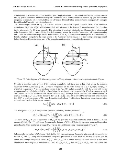
Figure 13. Polar diagram of Sc illustrating numerical integration procedures; z-axis equivalent to the X3 axis.
Consider a modulus vector E1 (i.e. 1/ S 33 ) making an angle θ1 with the z-axis in Fig 13(a), where the z-axis is
equivalent to the X3 axis in Fig. 10. The vector components on the x and z axes are (E1)x = E1sin(θ1) and (E1)z =
E1cos(θ1), respectively. A second modulus vector E2 in Fig.13(b) makes an angle θ2 with the z-axis with vector
components (E2)x = E2sin(θ2) and (E2)z = E2cos(θ2) on the x-axis and z-axis, respectively. If both vectors are rotated
360 o around the z-axis two circles are formed of radius (E1)x and (E2)x which enclose a disc shaped volume of
average radius [(E1)x + (E2)x]/2 and thickness Δz = [(E1) - (E2)z] Thus, if θ is allowed to increase from 0 to π radians
(i.e. 180 o ) in small increments of Δθ (~one degree) the total volume VE of the three dimensional polar diagram is the
summation of a series of disc shaped volumes:
2
V E [( E1
) z ( E2)
z][(
E1)
x ( E2)
x]
(21)
4
0
477
O
z
2
(E 2)
x
The average radius (Eav)1 of an equivalent sphere of volume VE is readily obtained:
1/
3
3
2
( ) 1 3 / 4
[(
1)
( 2)
][( 1)
( 2)
]
16
0
E av VE
E z E z E x E x
(22)
The value of (Eav)1 in (22) is equivalent to (Eav)1 in Eq. (19) and calculated results are listed in Table 7. In like
manner, (Gav)1 in Eq. (19) is obtained from the polar diagram of G (i.e. 1 / S G ) using the same numerical integration
procedures to obtain a spherical average (Gav)1 via Eq. (23), and the resulting values included in Table 7
1/
3
3
2
( ) 1 3 / 4
[(
1)
( 2)
][( 1)
( 2)
]
16
0
G av VG
G z G z G x G x
(23)
Subsequently, the values of (Eav)2 and (Gav)2 in Eq. (20) were determined from polar diagrams of the compliance
vectors S 33 and S G , using similar numerical integration procedures to those described for Eqs. (22) and (23) to
obtain the average compliance radius, ( S 33)
av and ( S G)
av , of a sphere having the same volume as the three
dimensional polar diagram of compliances. Thus, 1/( S 33 ) av ( Eav)
2 and 1/( S 44 ) av ( Gav)
2 , and their values are
E
2
z
(E )
2 z
1/
3
1/
3
x