elastic anisotropy of hcp metal crystals and polycrystals

IJRRAS 6 (4) ● March 2011 www.arpapress.com/Volumes/Vol6Issue4/IJRRAS_6_4_14.pdf 

ELASTIC ANISOTROPY OF HCP METAL CRYSTALS 

AND POLYCRYSTALS 

Desmond Tromans 

Department of Materials Engineering, University of British Columbia, Vancouver BC, Canada V6T 1Z4 

E-mail: dtromans@interchange.ubc.ca 

ABSTRACT 

The monocrystal elastic behaviours of twenty four hexagonal close packed (HCP) metals at room temperature are 

reviewed based on published values of their monocrystal elastic constants. In particular, the angular variation of the 

Young’s Modulus (E) and the Rigidity (Shear) Modulus (G) are determined using general equations developed by 

Voigt [1928] and comparisons between the different metals presented graphically. The consequences of anisotropic 

monocrystal behaviour on the elastic behaviour of polycrystals composed of randomly oriented grains (crystal 

aggregates) are explored using a three dimensional spherical analysis together with the analytical methods of Voigt 

[1889] and Reuss [1929], and comments made on the consequences of non-randomly oriented grains. 

Keywords: Matrices, stiffness, compliance, Young’s modulus, shear modulus, texture. 

1. INTRODUCTION 

There is considerable experimental information on the elastic constants of metal monocrystals and mineral crystals. 

However, a comparative examination of behaviour between all HCP metals stable at room temperature, particularly 

a single source graphical comparison, is both desirable and useful. The physics upon which elastic constants are 

based and the relationships between the constants and crystallography are well established. However, the language 

of crystal physics is somewhat complex, involving conventions and procedures which are not immediately obvious 

to the non-specialist. Consequently, some general comments relating to the basic terminologies of stresses and 

strains, tensors and matrices, and crystal structure are presented first, followed by an examination of the elastic 

behaviour of HCP monocrystals and subsequent effects on polycrystals. 

2. BASIC TERMINOLOGY 

2.1. Stress and Strain. 

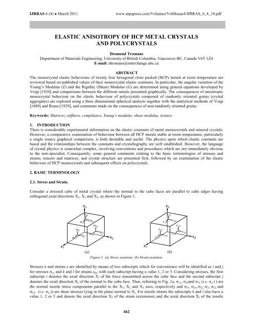
Consider a stressed cube of metal crystal where the normal to the cube faces are parallel to cube edges having 

orthogonal axial directions X1, X2 and X3, as shown in Figure 1. 

x 1 

11 

31 

13 

x 3 

21 

33 

23 32 12 

22 

x 2 

(a) (b) 

Figure 1. (a) Stress notation; (b) Strain notation. 

Stresses σ and strains ε are identified by means of two subscripts which for convenience will be identified as i and j 

for stressesijand k and l for strains εkl, with each subscript having a value 1, 2 or 3. Considering stresses, the first 

subscript i denotes the axial direction Xi of the force transmitted across the cube face and the second subscript j 

denotes the axial direction Xj of the normal to the cube face. Thus, referring to Fig. 1a, σ11, σ22and σ33 (i.e. σiiare 

the normal tensile stress components parallel to the X1, X2 and X3 axes, respectively and and 

(i.e. ij are shear stresses lying in the plane normal to Xj. For tensile strains the subscripts k and l also have a 

value 1, 2 or 3 and denote the axial direction Xk of the strain (extension) and the axial direction Xl of the tensile 

462 

x 1 

11 

31 

13 

x 3 

21 

33 

23 

32 

12 

22 

x 2

IJRRAS 6 (4) ● March 2011 Tromans ● Elastic Anisotropy of Hcp Metal Crystals and Polycrystals 

force. Consequently, referring to Fig. 1b, and (i.e. kk) are tensile strains (fractional extensions) parallel 

to the X1, X2 and X3 axes, respectively. The shear strains kl are due to a rotation towards the Xk axis of a line 

element parallel to the Xl axis. For example, 23 indicates a rotation towards the X2 axis of a line element parallel to 

the X3 axis, which obviously involves a rotation about the third axis X1 

. 

X 3 

23 

23= 32 = 

32 

X 3 

 

X2 X2 (a) (b) 

Figure. 2. Relationship between (a) tensor shear strain pairs and (b) engineering shear strain . 

463 

= 23+ 32 The shear strains are angles measured in radians. For example, if a pure shear stress (torque) is applied to cause a 

rotation about the X1 axis the resulting pure shear strains 23 and 32 are shown in Fig. 2. Note that the engineering 

shear strain is the sum of the shear strains 23 + 32. The consequences of this are discussed later in relation to 

compliances. 

2.2. Elastic Stiffness and Compliance. 

Elastic materials exhibit a proportional relationship between an applied stress and the resulting tensile strain , 

provided the strains are smallThe resulting linear relationship is known as Hooke’s Law. In engineering, the 

constant of proportionality is known as the tensile elastic modulus E (Young’s Modulus) and the usual form of the 

relationship is given by Eq. (1) where is a uniaxial stress and is the strain elongation in the direction of the 

applied stress: 

= E 1) 

In fact, Equation 1 describes a uniaxial stress situation with three dimensional strains (elongation strain plus lateral 

strains dependent upon Poisson’s ratio) and is more formally stated in elasticity in terms of the compliance S with 

as the dependent variable: 

= S (2) 

where S is the reciprocal Young’s Modulus (1/E). 

In analogous manner, a three dimensional stress situation with uniaxial strain is expressed in terms of the stiffness C 

with the stress in the direction of uniaxial strain being the dependent variable: 

= C 

2.3. Tensors and Matrices. 

Note that in general C ≠ E. and the elastic relationship between stresses and strains in crystals must be stated in a 

more generalized manner: 

C and S 

(4) 

ij ijkl kl 

kl klij ij 

In Eq. (4), Cijkl are stiffness constants of the crystal and Sklij are the compliances of the crystal and both are a fourth 

rank tensor (Wooster, 1949; Nye, 1985). Figure 1 shows there are nine forms of ij and nine forms of kl so that the 

generalized Eq. (4) leads to 81 Cijkl stiffness coefficients and 81 Sklij compliance coefficients which form a fourth 

rank tensor represented by a symmetrical 9 x 9 array of coefficients. Thus, Eq. (4) becomes: 

11 

C 

 

 

22 

 

C 

 

33 C 

 

23 

C 

 

 

31 C 

 

12 

C 

 

 

32 

 

C 

 

 

13 C 

 

 

21 

 

C 

1111 

2211 

3311 

2311 

3111 

1211 

3211 

1311 

2111 

C 

C 

C 

C 

C 

C 

C 

C 

C 

1122 

2222 

3322 

2322 

3122 

1222 

3222 

1322 

2122 

Full tensor notation Full tensor notation 

C1133 

C1123 

C1131 

C1112 

C1132 

C1113 

C1121 

11 

 

 

C 

 

2233 C2223 

C2231 

C2212 

C2232 

C2213 

C2221 

22 

C 

 

 

3333 C3323 

C3331 

C3312 

C3332 

C3313 

C3321 

33 

 

 

C2333 

C2323 

C2331 

C2312 

C2332 

C2313 

C2321 

23 

C 

 

 

3133 C3123 

C3131 

C3112 

C3132 

C3113 

C3121 

31 

 

C1233 

C1223 

C1231 

C1212 

C1232 

C1213 

C1221 

12 

 

 

 

C3233 

C3223 

C3231 

C3212 

C3232 

C3213 

C3221 

 

32 

 

C 

 

 

1333 C1323 

C1331 

C1312 

C1332 

C1313 

C1321 

13 

 

 

C2133 

C2123 

C2131 

C2112 

C2132 

C2113 

C2121 

 

21 

11 

S1111 

S1122 

S1133 

S1123 

S1131 

S1112 

S1132 

S 

 

 

22 

 

S2211 

S2222 

S2233 

S2223 

S2231 

S2212 

S2232 

S 

 

33 S3311 

S3322 

S3333 

S3323 

S3331 

S3312 

S3332 

S 

 

23 

S 

2311 S2322 

S2333 

S2323 

S2331 

S2312 

S2332 

S 

 

 

31 S3111 

S3122 

S3133 

S3123 

S3131 

S3112 

S3132 

S 

 

12 

S1211 

S1222 

S1233 

S1223 

S1231 

S1212 

S1232 

S 

 

 

32 

 

S3211 

S3222 

S3233 

S3223 

S3231 

S3212 

S3232 

S 

 

 

13 S1311 

S1322 

S1333 

S1323 

S1331 

S1312 

S1332 

S 

 

 

21 

 

 

S2111 

S2122 

S2133 

S2123 

S2131 

S2112 

S2132 

S 

1113 

2213 

3313 

2313 

3113 

1213 

3213 

1313 

2113 

S 

1121 

S 

S 

S 

S 

S 

S 

S 

S 

2221 

3321 

2321 

3121 

1221 

3221 

1321 

2121 

 

 

 

 

 

 

 

 

 

 

 

 

 

 

 

 

 

 

11 

22 

33 

23 

31 

12 

32 

13 

21 

 

 

 

 

 

 

 

 

 

 

 

 

 

 

(5)


The physical meaning of each Cijkl is obtained by considering a set of applied stress components where all 

components of strain vanish except for either one normal component or a pair of shear components. An example 

with one normal component of strain is 11 =C111111 (i.e. ii =Ciikk where i= k). A situation corresponding to one 

pair of tensor shear components is = C232323 + C233232 (where i ≠ j, k ≠ l) Similarly, the meaning of each Sijkl is 

obtained by considering a set of applied strain components where all components of stress vanish except for either 

one normal component or a pair of shear components. An example with one normal component of stress is given by 

the situation where 11 =S111111 (i.e. ii =Siikk where i= k). The situation corresponding to one pair of shear stress 

components is given by = S232323 + S233232 (where i ≠ j, k ≠ l). 

The number of suffixes on the stiffness and compliance may be decreased by considering the static equilibrium of a 

stressed cube in Fig. 1. It is evident that 12 = 21, 13= 31 and 23 = 32 otherwise rotations occur. Similarly, 12 = 

21, 13 = 31 and 32 = 23. The ability to interchange suffixes i and j in ij, and suffixes k and l in kl, implies that it is 

unnecessary to distinguish between i and j or between k and l (e.g. = Consequently, following 

from Voigt [1928)], it has become common practice to use a contracted matrix notation with single number suffixes 

instead of pairs. The relationship between pairs (ij or kl) and single numbers (m or n) is shown below: 

ij or kl 11 22 33 23,32 31,13 12,21 

↓ ↓ ↓ ↓ ↓ ↓ 

m or n 1 2 3 4 5 6 

Equation (5) may now be rewritten as Eq. (6) in the contracted tensor notation where the engineering shear strain 

= (+32), = (+13) and = (+11), according to Fig. 2. Also, using the contracted notation 

 

and 

Contracted tensor notation Contracted tensor notation 

1 

C11 

C12 

C13 

C14 

C15 

C16 

C14 

C15 

C16 

1 

 

 

 

 

 

2 

 

C12 

C22 

C23 

C24 

C25 

C26 

C24 

C25 

C26 

 

2 

 

 

 

 

 

3 C13 

C23 

C33 

C34 

C35 

C36 

C34 

C35 

C36 

3 

 

 

 

4 

C14 

C24 

C34 

C44 

C45 

C46 

C44 

C45 

C46 

 

4 / 2 

 

 

 

/ 2 

5 C15 

C25 

C35 

C45 

C55 

C56 

C45 

C55 

C56 

5 

 

 

 

6 

C16 

C26 

C36 

C46 

C56 

C66 

C46 

C56 

C66 

 

6 / 2 

 

 

 

 

4 

 

C14 

C24 

C34 

C44 

C45 

C46 

C44 

C45 

C46 

 

4 / 2 

 

 

 

 

/ 2 

5 C15 

C25 

C35 

C45 

C55 

C56 

C45 

C55 

C56 

5 

 

 

 

 

6 

 

 

C16 

C26 

C36 

C46 

C56 

C66 

C46 

C56 

C66 

 

 

6 / 2 

1 

S11 

S12 

S13 

S14 

S15 

S16 

S14 

S15 

S16 

1 

 

 

 

 

 

2 

 

S12 

S22 

S23 

S24 

S25 

S26 

S24 

S25S26 

 

2 

 

 

 

 

 

3 S13 

S23 

S33 

S34 

S35 

S36 

S34 

S35 

S36 

3 

 

 

 

 

4 / 2 

S14 

S24 

S34 

S44 

S45 

S46 

S44 

S45S46 

 

4 

 

 

 

 

5 / 2 S15 

S25 

S35 

S45 

S55 

S56 

S45 

S55 

S56 

5 

 

 

 

 

6 / 2 

S16 

S26 

S36 

S46 

S56 

S66 

S46 

S56S66 

6 

 

 

 

 

 

4 / 2 

 

S14 

S24 

S34 

S44 

S45 

S46 

S44 

S45S46 

 

4 

 

 

 

 

 

5 / 2 S15 

S25 

S35 

S45 

S55 

S56 

S45 

S55 

S56 

5 

 

 

 

 

6 

/ 2 

 

S16 

S26 

S36 

S46 

S56 

S66 

S46 

S56 

S66 

 

6 

 

After summing each tensor equation represented in Eq. (6) it becomes evident that all the relationships between 

stresses, strains, and stiffness coefficients, and strains, stresses and compliance coefficients, may each be represented 

by a symmetrical 6x6 matrix as shown in Eq. (7): 

C- Matrix S- Matrix S-Matrix, -factors included 

1 

C11 

C12 

C13 

C14 

C15 

C16 

1 

 

 

 

 

 

2 

 

C12 

C22 

C23 

C24 

C25 

C26 

 

2 

 

 

 

 

 

3 C13 

C23 

C33 

C34 

C35 

C36 

3 

 

 

 

4 

C14 

C24 

C34 

C44 

C45 

C46 

 

4 

 

 

 

 

5 C15 

C25 

C35 

C45 

C55 

C56 

5 

 

 

 

 

6 

 

 

C16 

C26 

C36 

C46 

C56 

C66 

 

 

6 

 

1 

S11 

S12 

S13 

2S14 

2S15 

2S16 

1 

 

 

 

 

 

2 

 

S12 

S22 

S23 

2S24 

2S25 

2S26 

 

2 

 

 

 

 

 

3 S13 

S 23 S33 

2S34 

2S35 

2S36 

3 

 

 

 

 

4 2S14 

2S24 

2S34 

4S44 

4S45 

4S46 

4 

 

 

 

 

 

5 2S15 

2S25 

2S35 

4S45 

4S55 

4S56 

5 

 

 

 

 

6 

 

 

2S16 

2S26 

2S36 

4S46 

4S56 

4S 

66 

 

6 

 

1 

S11 

S12 

S13 

S14 

S15 

S16 

1 

 

 

 

 

 

2 

 

S12 

S22 

S23 

S24 

S25 

S26 

 

2 

 

 

 

 

 

3 S13 

S 23 S33 

S34 

S35 

S (7) 

36 3 

 

 

 

 

4 S14 

S24 

S34 

S44 

S45 

S46 

 

4 

 

 

 

 

5 S15 

S25 

S35 

S45 

S55 

S56 

5 

 

 

 

 

6 

 

 

S16 

S26 

S36 

S46 

S56 

S 66 

 

6 

 

When the pairs of suffixes mn on the matrix shear compliances, Smn are such that m or n are both 4, 5, or 6 the 

compliance Smn is multiplied by a factor () of 4 (e.g. 4S45, and 4S56). When either m or n are 4, 5, or 6 the 

compliance Smn is multiplied by a factor () of 2 (e.g. 2S16, 2S35, 2S24). All other compliances have a multiplying 

factor of unity. The consequences are such that it is standard recommended practice [Voigt 1928; Nye 1985] when 

using or measuring compliance values that the multiplying factor ( ) is always included in the reported value (e.g. it 

is implicit S44 = 4S44). All compliance values reported in the present study follow this practice. [N.B. Wooster’s 

[1949] treatment does not include multiplying factors of 2 or 4 in his reported S values. They must be applied later.] 

2.4. Effects of Crystal Symmetry on C and S Matrices. 

The number of independent coefficients in the 6 x 6 matrix array is reduced from 36 to 21 by a centre of symmetry 

(e.g. C12 = C21, C13 = C31 ….; S12 = S21, S13 = S31…, etc.) as evident in Eq. (7), and is further reduced by other 

symmetry elements such as axes of rotation, mirror planes and inversion such that some constants are zero and 

464 

(6)


others have equal values. The resulting effect for hexagonal crystal structures of all classes is to reduce the number 

of independent elastic constants to six [Voigt, 1928; Nye, 1985; Hearmon, 1979], as shown in the symmetrical 6 x 6 

matrices in Eq. (8): 

1 

C11 

C12 

C13 

1 

1 

S11 

S12 

S13 

1 

 

 

 

 

 

2 

 

C12 

C11 

C 

 

 

 

 

 

13 

2 

2 

 

S12 

S11 

S13 

 

 

2 

 

 

 

 

3 C13 

C13 

C33 

3 

 

 

 

3 S13 

S13 

S33 

3 

 

 

 

 

 

(8) 

4 

 

C44 

 

4 

 

4 

 

S44 

4 

 

 

 

 

 

5 

C 

 

 

 

44 

5 

 

 

 

 

5 S44 

5 

 

 

 

 

6 

 

 

C66 

 

6 

 

 

6 

 

 

S66 

 

6 

 

C66 ( C11 

C12) 

/ 2 

S66 2( S11 

S12) 

The 6 x 6 matrices in Eq. (8) are related to each other via matrix inversion. Consequently if the compliances (Smn) 

are known then the corresponding stiffness constants (Cmn) may be obtained via matrix inversion and vice versa. 

This is important because initial compliance measurements were most easily measured via static techniques such as 

bending and torsion tests [Hearmon, 1946] whereas stiffness may not be measured in this manner (e.g. it is difficult 

to conduct a static tensile test for a uniaxial strain situation because three orthogonal stresses are necessary). 

However, experiments involving propagation of longitudinal and transverse elastic waves allow measurement of the 

Cmn because the tensile stiffness in a specific direction is related to the density of the test material and the velocity of 

the longitudinal wave in the same direction [Rowland and White, 1972; Gebrande, 1982; Blessing, 1990; Lim et al. 

2001]. Similarly, the shear stiffness on a specific plane is related to the velocity of the shear wave on that plane and 

the density of the test material. 

3. METAL HCP CRYSTALS 

3.1. Crystallography. 

The crystallographic nature of the hexagonal metal structures is shown in Fig. 3. The unit cell in (a) has two axes a1 

and a2 of equal length inclined at 60 o , and an orthogonal axis of different length c. Fig. 3(b) shows the principal 

crystallographic directions in the (0001) basal plane expressed in the Miller-Bravais system [Cullity, 1956] using 

four axes composed of three planar a-axes (a1 = a2 = a3) at 120 o to each other and the orthogonal c-axis. Fig 3(c) 

shows the relationship between the orthogonal X-axes in Fig. 1 and crystallographic directions. 

a 1 

c 

a 2 

a 1 

90 o 

c 

90 o 

120 o 

a 2 

- [1210] 

-- 

[1120] - [2110] 

a 3 

465 

- [1100] 

- - [1210] 

- [0110] 

a 2 

x 1 

90 o 

[0001] 

x3 o 

90 o 

90 o 

x2 - [0110] 

a 1= a 2= a3 

[2110] -- 

a1 - [1010] 

- [1120] 

-- 

[2110] 

(a) (b) (c) 

Figure 3 HCP metal crystallography.(a) Unit cell showing the a1, a2, and c-axes. (b) Directions in Miller-Bravais indices. 

(c) Relationship between X1, X2 and X3 axes in Figure 1 and crystallographic directions. 

When defining and measuring compliance and stiffness constants it is most important that the orthogonal axes X1 X2 

and X3 in Fig.1 conform to standardised orthogonal directions in the HCP crystals (Nye). These directions are shown 

in Fig 3(c) where X1 = [ 21 

10] 

i.e. the a1-axis, X2 = [ 011 

0] 

and X3 = [0001] i.e. the c-axis. All S and C constants 

are reported with respect to these axial directions. For example in Fig.1, and correspond to tensile stresses 

and strains in the [0001] direction and S33 and C33 correspond to the compliance and stiffness constants, respectively, 

measured in the [0001] direction. 

3.2. HCP Metals Examined. 

Twenty four hexagonal structured metals with an atomic number (At. No.) ranging from 4 to 81were examined. All 

belong to the crystal class P63/mmc. They are listed in Table 1 in order of their At. No., together with their c/a ratio 

and density (ρ) obtained from Metals Handbook [1985]. The ideal c/a ratio required for close packing of spheres to 

form the HCP structure is 1.633 (i.e. 24 / 3).


At. 

No. 

Table 1. Hexagonal crystals studied with c/a ratio and density ρ. 

Metal c/a ρ 

(g cm -3 ) 

466 

At. 

No. 

Metal c/a ρ 

(g cm -3 ) 

4 Be α-Beryllium 1.56803 1.85 60 Nd α-Neodymium ‡ 3.22404 7.00 

12 Mg Magnesium 1.62350 1.74 64 Gd α-Gadolinium 1.58791 7.86 

21 Sc α-Scandium 1.59215 2.9 65 Tb α-Terbium 1.58056 8.25 

22 Ti α-Titanium 1.58734 4.51 66 Dy α-Dysprosium 1.57382 8.55 

27 Co α-Cobalt 1.62283 8.85 67 Ho α-Holmium 1.56983 8.79 

30 Zn Zinc 1.85635 7.13 68 Er α-Erbium 1.52877 9.15 

39 Y α-Yttrium 1.56986 4.47 69 Tm α-Thulium 1.57932 9.31 

40 Zr α-Zirconium 1.59312 6.49 71 Lu α-Lutetium 1.57143 9.85 

44 Ru Ruthenium 1.58330 12.45 72 Hf α-Hafnium 1.58147 13.1 

48 Cd Cadmium 1.88572 8.65 75 Re Rhenium 1.61522 21.0 

57 La α-Lanthanum ‡ 3.22546 6.15 76 Os Osmium 1.57993 22.61 

59 Pr α-Praseodymium ‡ 3.22616 6.77 81 Tl α-Thallium 1.59821 11.85 

Three metals La, Pr and Nd have the DHCP (double HCP) structure where the stacking of close packed planes 

follows the order ABACABAC instead of the usual HCP sequence ABAB [Nareth, 1969]. Consequently, close 

packing under these conditions leads to an ideal c/a ratio of 3.3256. Overall, most of the metals were lower and 

within -0.1 of their ideal c/a ratio, except for Cd and Zn which exceeded the ratio by 0.223 and 0.194, respectively. 

Values for the five independent stiffness and compliance constants of all twenty four hexagonal metals were 

obtained from the published literature and listed in Table 2. Most were obtained from the data compiled by Hearmon 

[1979]. Additionally, as noted at the foot of Table 2, constants for the metals La, Os, Tm and Tl were obtained from 

(a) Ouyang et al. [2009], (b) Pantea et al. [2008], (c)Lim et al. [2001] and Singh [1999], and (d) the combined 

averages of Ferris et al. [1963] and Weil and Lawson [1966]. A matrix inversion of C to S, and vice versa (see Eq. 

(8)), was conducted by the author to confirm consistency between the stiffness and compliance values. In some 

instances only C-values were measured and reported, in which case the author used matrix inversion to obtain the 

corresponding S-values. In the case of La no experimental measurements were available, possibly due to the 

difficulty of growing single crystals of the DHCP -phase which were free from the metastable FCC -phase phase 

at room temperature [Stassis et al.1982, Dixon et al. 2008]. Consequently, the theoretical stiffness calculations of La 

by Ouyang et al [2009] were employed because their work shows reasonable correlation between measured and 

theoretical values in other hexagonal metal crystals. 

Table 2. Stiffness and Compliance Data. Hearmon [1979], unless indicated otherwise. 

Metal Stiffness Constants (GPa) Compliance Constants (TPa) -1 

C11 C33 C44 C12 C13 S11 S33 S44 S12 S13 

Be 292 349 163 24 6 3.45 2.87 6.14 -0.28 -0.05 

Mg 59.3 61.5 16.4 25.7 21.4 22.0 19.7 60.98 -7.75 -4.96 

Sc 99.3 107 27.7 39.7 29.4 12.46 10.57 36.1 -4.32 -2.24 

Ti 160 181 46.5 90 66 9.62 6.84 21.5 -4.67 -1.81 

Co 295 335 71 159 111 4.99 3.56 14.08 -2.36 -0.87 

Zn 165 61.8 39.6 31.1 50 8.07 27.55 25.25 0.606 -7.02 

Y 77.9 76.9 24.3 29.2 20 15.44 14.4 41.15 -5.10 -2.69 

Zr 144 166 33.4 74 67 10.20 8.01 29.94 -4.09 -2.46 

Ru 563 624 181 188 168 2.09 1.82 5.525 -0.576 -0.408 

Cd 116 50.9 19.6 43 41 12.20 33.76 51.02 -1.32 -8.763 

La (a) 

51.44 54.63 13.92 17.27 10.4 22.35 19.42 71.84 -6.91 -2.94 

Pr 49.4 57.4 13.6 23 14.3 26.60 19.32 73.53 -11.28 -3.82 

Nd 54.8 60.9 15.0 24.6 16.6 23.66 18.53 66.66 -9.45 -3.87 

Gd 67.25 71.55 20.75 25.3 21 18.15 16.12 48.19 -5.686 -3.659 

Tb 68.55 73.3 21.6 24.65 22.4 17.68 16.0 46.30 -5.10 -3.84 

Dy 74 78.6 34.3 25.5 21.8 16.03 14.48 41.15 -4.59 -3.17 

Ho 76.5 79.6 25.9 25.6 21 15.32 14.1 38.60 -4.33 -2.90 

Er 84.1 84.7 27.4 29.4 22.6 14.10 13.2 36.50 -4.21 -2.63 

Tm (c) 

92.5 81.5 28.2 33.5 21 12.82 13.42 35.46 -4.133 -2.237 

Lu 86.2 80.9 26.8 32 28 14.28 14.79 37.30 -4.17 -3.50 

Hf 181 197 55.7 77 66 7.15 6.13 18.0 -2.47 -1.57 

Re 616 683 161 273 206 2.11 1.70 6.210 -0.804 -0.394 

Os (b) 

765 846 270 229 219 1.501 1.334 3.704 -0.365 -0.294 

Tl (d) 

41.35 53.85 7.23 36 29.45 104.5 31.80 138.3 -82.40 -12.12 

(a) Ouyang et al. [2009]: (b) Pantea et al. [2008], (c) Lim et al. [2001] except C13 which is the average of the 

interpolated value of 25 GPa by Lim et al. [2008] and a calculated value of ~17 GPa by Singh [1999]: (d) Average 

of data from Ferris et al [1963] and Weil and Lawson [1966].


3.3 Stiffness. 

The most important aspect of uniaxial strain conditions is the three dimensional stress state where the presence of 

lateral tensile stresses allows no lateral strain contractions i.e. Poisson’s ratio is zero. This is readily evident from an 

examination of the stiffness (C) relationships in Eq. (8), leading to Eq. (9), for uniaxial strains and 

: ( 

1 

2 

3 

2 

: ( 

1 

: ( 

1 

3 

3 

2 

 

 

0) 

: 

0) 

: 

0) 

: 

C 

 

1 

2 

3 

C 

11 11 

11 

33 

 

2 

3 

467 

, 

, 

 

2 

1 

1 

C , C 

12 

C 

12 

13 

1 

2 

3 

, 

3 

3 

2 

13 1 

C 

C , C , C 

3.4 Young’s Modulus E and Rigidity (Shear) Modulus G. 

The tensile modulus E is the constant of proportionality between stress and strain under uniaxial stress loading as 

measured in the direction of the applied stress (i.e. a three dimensional strain situation). It has wide application in 

engineering design. Examination of the compliance (S) relationships in Eq. (8) under a uniaxial stress or 3 

yields the relationships shown in Eq. (10) where it is evident that E is the reciprocal compliance S -1 : 

: ( 

1 

2 

3 

2 

1 

: ( 

1 

3 

: ( 

3 

2 

 

 

 

0) 

: 

0) 

: 

0) 

: 

E 

E 

E 

( 21 

10) 

( 011 

0) 

( 0001) 

/ ( S 

 

3 

1 

2 

1 

/ 

3 

2 

( S 

/ ( S 

) 

1 

11 

1 

11 

) 

) 

1 

33 

 

 

 

1 

2 

1 

12 

12 

13 

2 

3 

13 

13 

S , S 

1 

2 

3 

3 

3 

2 

13 

S , S 

13 

S , S 

The subscripts ( 21 

10) 

, ( 011 

0) 

and (0001) in Eq. [10] refer to the crystal plane lying normal to the direction of 

the uniaxial stress (see Figs. 3 and 4) and the corresponding E values are listed in Table 3. 

(0001) 

(0110) 

(2110) 

(1011) 

(a) (b) (c) (d) (e) 

13 

1 

2 

3 

(1121) 

Figure 4. Orientations and Miller-Bravais indices of principal planes in hexagonal crystals (a) basal plane, (b) primary 

prismatic plane: (c) secondary prismatic plane: (d) primary pyramidal plane and (e) secondary pyramidal plane. 

For uniaxial stresses and 3 the corresponding average Poisson’s ratios, 1 2 and 3 are obtained: 

( 

2 

3) 

( 

S12 S13) 

( 

1 

3) 

( 

S12 

S13) 

( 

2 

1) 

( 

S13 

S13) 

1 ; 2 

; 3 

; (11) 

2 

2S 

2 

2S 

2 

2S 

1 

11 

2 

The negative sign in the formulae for Poisson’s ratio in Eq. (11) is introduced because the lateral strains are usually 

contractions (negative strain) and it is conventional to express as a positive number. Note that the ratios of the two 

components S12/S11 and S13/S11 in and 2 are unequal leading to different lateral strains in orthogonal directions X1 

and X3 in the ( 21 

10) 

prismatic plane and orthogonal directions X2 and X3 in the ( 011 

0) 

prismatic plane (see Figs. 

3 and 4). Zinc is an unusual metal because S12 has a positive value (see Table 2) indicating that there is an expansion 

along the c-axis in the X3 direction on the prismatic planes (i.e. a negative of -S12/S11 = -0.075 in the X3 direction). 

Similar negative -values on prismatic planes of Zn have been reported previously [Lubarda and Meyers, 1999] 

Although uncommon, negative -values are not forbidden by thermodynamics and have been reported for several 

metal crystals of cubic symmetry when stretched in the [110] direction [Baughman et al., 1998] and in the mineral 

cristobalite [Yeganeh-Haeri et al. 1992]. Based on Eq. (11) average values of Poisson’s ratio 1 and 2 on the 

prismatic planes, and 3 on the basal plane, are listed in Table 3. 

Conditions of pure shear are produced under torsional loading where the stresses involved are readily seen by an 

examination of Figs. 1, 3 and 4. If torsion is produced on the ( 21 

10) 

prismatic plane by rotation around the X1 axis 

the shear stresses involved are 31 and 21 (i.e. 5 and 6 in the contracted notation). Similarly, torsion produced on 

11 

3 

33 

(9) 

(10)


the 011 

0) 

( prismatic plane by rotation around the X2 axis involves the shear stresses 32 and 12 (i.e. 4 and 6), 

whereas torsion on the (0001) basal plane via rotation around the X3 axis requires the shear stresses 13 and 23 (i.e. 

4 and 5). Consequently, from Eq.(12), the average shear compliances SG on the ( 21 

10) 

, ( 011 

0) 

and (0001) 

planes are obtained: 

5 / 5 

6 

/ 6 

S55 

S66 

S44 

2S11 

2S12 

 

SG 

( 21 

10) 

 

2 

 

2 

 

2 

 

 

 

 

4 / 4 

6 

/ 6 

S44 

S66 

S44 

2S11 

2S12 

 

SG 

( 011 

0) 

 

2 

 

2 

 

2 

 

(12) 

 

 

 

4 / 4 

5 

/ 5 

S44 

S55 

 

SG 

 

S 

( 0001) 

 

44 

2 

 

2 

 

 

 

Hence, the shear modulus G on each crystal plane is simply the reciprocal compliance (SG) -1 and is listed in Table 3 

for the different hexagonal metal crystals. 

 

Table 3. Young’s Modus (E ), Poisson’s Ratio and Shear Modulus (G ) 

E , E 

( 21 

10) 

( 011 

0) 

E ( 0001) 

( 1 ) , ( 2) 

 

( 21 

10) 

( 011 

0) 

3 ( 0001) 

Metal 

(GPa) (GPa) 

) ( G , G 

( 21 

10) 

( 011 

0) 

G ( 0001) 

(GPa) (GPa) 

Be 290 348.4 0.0479 0.0174 147.1 162.3 

Mg 45.5 50.76 0.289 0.252 16.6 16.4 

Sc 80.3 94.67 0.263 0.212 28.7 27.7 

Ti 104 146.2 0.337 0.265 39.9 46.5 

Co 200 280.9 0.324 0.244 69.5 71.0 

Zn 124 36.3 0.397 0.255 49.8 39.6 

Y 64.8 69.44 0.252 0.187 24.3 24.3 

Zr 98 124.8 0.321 0.307 34.2 33.4 

Ru 478 549.5 0.235 0.224 184.2 181 

Cd 82 29.62 0.413 0.259 25.6 19.6 

La (a) 

44.7 51.49 0.220 0.151 15.3 13.9 

Pr 37.6 51.76 0.284 0.198 13.4 13.6 

Nd 42.3 53.97 0.281 0.209 15.1 15.0 

Gd 55.1 62.04 0.257 0.227 20.9 20.8 

Tb 56.6 62.5 0.253 0.240 21.8 21.6 

Dy 62.4 69.06 0.242 0.219 24.3 24.3 

Ho 65.3 70.92 0.236 0.206 25.7 25.9 

Er 70.9 75.76 0.243 0.199 27.4 27.4 

Tm (c) 

78 74.5 0.248 0.167 28.8 28.2 

Lu 70 67.6 0.269 0.237 27.0 26.8 

Hf 140 163.1 0.283 0.256 53.7 55.6 

Re 474 588.2 0.284 0.232 166 161 

Os (b) 

666 749.6 0.220 0.220 269 270 

Tl (d) 

9.57 31.45 0.452 0.381 3.91 7.23 

3.5 Representation of Angular Anisotropy of E and G. 

While the magnitude and anisotropy of the elastic moduli is indicated in Table 3 for the three principal planes, it is 

desirable to know the full effect of differently oriented planes on the values of E and G in hexagonal crystals. For 

example, consider a plane which makes intercepts x, y and z on the X1 X2 and X3 axes, respectively, as shown in Fig. 

(5a). Let the direction of the normal (N) to this plane make an angel θ with respect to the X3 axis. The X1 X2 and X3 

axes are now rotated to the positions 1 X , 2 X and 3 X while remaining orthogonal so that the angle between X3 and 

X 3 is θ, as shown in Fig. 5(b). It is evident from Eq. (10) that the tensile compliance on the xyz plane is S 33 with a 

corresponding tensile modulus 

S 

S 

) / 2 and 

E ( S 

. Similarly, from Eq. (12), the shear compliance on the same plane is 

 

 

1 

33) 

SG ( 44 55 

1 

G ( SG 

) , where S 33 , S 44 and S 55 are calculated with respect to the new (transformed) 

axes 1 X , 2 X and 3 X . [N.B. While S44 = S55 when using the standard X1 X2 and X3 axes as shown in Eq. (12), 

468


S 44 S 

55 when referred to the transformed axes [Voigt 1928]. Furthermore, transformation of compliances to the 

new axes must be conducted in the full tensor notation (see Eq. (5)) after which values may be converted to the 

contracted matrix notation [Nye 1985]. Transformation is a tedious procedure aided by the resulting cylindrical 

symmetry of the compliances with respect to the c-axis of the unit cell. Calculations of the transformed compliances 

were first conducted by Voigt [1928, pg. 746-747] to yield Eqs. (13) and (14): 

x 1 

x 

x3 

z 

y 

N 

x2 

469 

x 1' 

x1 -- 

[2110] 

[0001] 

x3 

o 

(a) (b) 

x3' 

- 

x2 [0110] 

Figure 5. (a) Direction (θ degrees) of the normal N to the plane xyz with respect to X3 (b) Transformed orthogonal axes X 1 , 

X 2 and 3 

X such that X3 is rotated by θ to coincide with N direction. 

4 

4 

2 2 

S S (sin ) 

S (cos ) 

( 2S 

S )(cos )(sin 

) 

(13) 

33 

11 

33 

13 

2 

2 2 

S ( 

G S S ) / 2 S ( S S 0. 

5S 

)(sin ) 

2( 

S S 2S 

S )(cos sin 

) 

(14) 

44 

55 

44 

11 

12 

44 

Voigt’s [1928] original equations were written in terms of cos 2 θ and (1-cos 2 θ). In Eqs. (13) and (14) the original (1cos 

2 θ) terms have been replaced by sin 2 θ. Note that when θ equals 0 o and 90 o 1 

, Eq. (13) shows that ( S is 

equivalent to (S33) -1 and (S11) -1 , respectively, consistent with Eq. (10). Similarly, in regard to Eq. (14), G 

equivalent to S44 when θ = 0 o , and S G is equivalent to ( S44 2S11 

2S12) 

/ 2 when θ = 90 o , consistent with Eq. (12). 

44 

11 

33 

13 

44 

x 2' 

33) 

S is 

1 

1 

Based on Eqs. (13) and (14), together with the relationships E ( S33) 

and G ( S 

G ) the angular variations of 

Young’s modulus (E ) and the shear modulus (G )for all metals listed in Table 1 may be represented graphically, via 

θ versus E and θ versus G diagrams . This is shown for the three metals Zn, Mg and Cd in Fig. 6 where the main 

consideration determining the combination was a reasonable similarity in magnitude between the E moduli and G 

moduli of each metal. It is readily evident that Zn and Cd are markedly anisotropic in behaviour, particularly Zn, 

whereas Mg tends to be considerably less anisotropic. Furthermore, the cylindrical symmetry of the behaviours of E 

and G with respect to the X3 axis (i.e. c-axis, [0001] direction) is evident in Fig 6, and evident in subsequent Figs. 7 

and 8, via the mirror image of the angular data on either side of the X3 axis. 

E (GPa) 

100 

50 

0 

Zn Zn 

Cd 

Mg 

X3 N - + N 

-90 -60 -30 0 30 60 90 

(degrees) 

Cd 

Mg 

G (GPa) 

50 

40 

30 

20 

10 

0 

Zn Zn 

Cd 

Mg 

X3 N - + N 

-90 -60 -30 0 30 60 90 

(degrees) 

Figure 6. Angular variation of E and G for Zn, Cd and Mg 

Cd 

Mg


The other twenty one metals investigated were also grouped in figures where there was a reasonable similarity in the 

magnitudes of the moduli. Thus, Fig. 7 shows the angular modulus behaviours of E and G for 0 o < θ < 90 for three 

groups of metals: Hf, Ti, Zr, Sc, and Y; Tm; Lu, Ho, Tb, and La; Er, Dy, Gd, Nd, Pr and Tl. 

E (GPa) 

200 

150 

100 

50 

0 

E (GPa) 

80 

60 

40 

20 

0 

Hf 

Ti 

Zr 

Sc 

Y 

X3 N - + N 

-90 -60 -30 0 30 60 90 

Lu 

Ho 

Tb 

La 

E (GPa) 

80 

60 

40 

20 

0 

(degrees) 

Tm Tm 

X3 N - + N 

-90 -60 -30 0 30 60 90 

Nd 

Pr 

(degrees) 

Er 

Dy 

Gd 

Tl 

X3 N - + N 

(degrees) 

Lu 

Ho 

Tb 

La 

Nd 

-90 -60 -30 0 30 60 90 

Pr 

470 

G (GPa) 

70 

60 

50 

40 

30 

20 

10 

0 

Y 

G (GPa) 

30 

20 

10 

0 

Hf 

Ti 

Zr 

Sc 

X3 N - + N 

-90 -60 -30 0 30 60 90 

Ho 

(degrees) 

Tm Tm 

Lu 

Lu 

Tb 

La 

G (GPa) 

30 

20 

10 

0 

X3 N - + N 

-90 -60 -30 0 30 60 90 

(degrees) 

Er 

Dy 

Gd 

Nd 

Pr 

(degrees) 

Y 

Ho 

Tb 

La 

Tl X3 Tl 

N - + N 

-90 -60 -30 0 30 60 90 

Figure 7. Angular variation of E and G for Hf, Ti, Zr, Sc and Y: Tm, Lu, Ho, Tb and La: Er, Dy Gd Nd Pr and La. 

As a general observation, with the exception Ti and Tl, E-behaviour in Fig 7 tends to exhibit a maximum on the 

(0001) basal plane (i.e. when θ is zero and N coincides with the [0001] direction) and a maximum (in most cases) on 

the prismatic planes where θ is 90 o . Additionally, in most cases, E tends to exhibit a minimum value between 0 o < θ 

< 90 o . In contrast, G tends to exhibit a minimum when θ is zero and 90 o , and a maximum for 0 o < θ < 90 o . In the case 

of Ti and Tl, the behaviours of E and G are similar, exhibiting a maximum when θ is zero and a minimum when θ is 

90 o . 

The group Os, Ru, Re, Be and Co exhibit the highest moduli of all the HCP metals and their collective behaviour is 

shown in Fig. 8. All show a pronounced maximum value of E on the basal plane, for which θ is zero, and a tendency 

by Ru, Re and Co to exhibit a minimum between 0 o < θ < 90. With the exception of Be, the G-behaviour exhibits a 

minimum when θ is zero and 90 o , and a maximum for 0 o < θ < 90 o . In the case of Be, a maximum G occurs when θ is 

zero, indicating G is highest on the basal plane. Overall, Figs 6 to 8 demonstrate a remarkably wide difference in the 

maximum E values in HCP metal crystals, ranging from an extremely high value of 749.6 GPa for Os (Fig. 8) to a 

low of 32.5 GPa for Tl (Fig. 7).


E (GPa) 

800 

700 

600 

500 

400 

300 

200 

100 

0 

Os Os 

Ru 

Re 

Re 

Be Be 

-90 -60 -30 0 30 60 90 

(degrees) 

Ru 

Co Co 

X3 N - + N 

471 

G (GPa) 

300 

250 

200 

150 

100 

50 

0 

Os Os 

Ru 

Re 

Be Be 

-90 -60 -30 0 30 60 90 

(degrees) 

Re 

Ru 

Co X3 Co 

N - + N 

Figure 8. Angular variation of E and G for Os, Ru, Re, Be and Co 

The presence and precise position of an intermediate maximum or minimum E at 0 < θ < 90 degrees in most of the 

graphical plots in Figs 6 to 8, due to a minimum or maximum in S 33 , was ascertained by differentiating Eq. (13) and 

placing the first differential equal to zero: 

S 

/ 

4S 

3 

sin cos 

4S 

3 

cos sin 

2( 

2S 

S 

33 

11 

o o 

with solutions 0 , 90 , and tan [( S 

33 

44 

13 

2S 

13 

44 

2S 

3 

3 

)(sin cos 

cos sin 

) 

0 

Similar procedures were applied to calculate the position of intermediate maxima/minima for G at 0< θ


Table 5. Calculate angles between the (0001) and selected (hkil) planes. 

Metal 

HCP 

c/a Ratio ( 101 

1) 

θ degrees 

( 1121) 

θ degrees 

( 101 

2) 

θ degrees 

( 1122) 

θ degrees 

( 101 

3) 

θ degrees 

( 2023) 

θ degrees 

Be 1.56803 61.09 72.31 42.15 57.47 31.11 50.36 

Mg 1.6235 61.92 72.88 43.15 58.37 32.00 51.34 

Sc 1.59215 61.46 72.57 42.59 57.87 31.50 50.79 

Ti 1.58734 61.38 72.52 42.50 57.79 31.42 50.70 

Co 1.62283 61.91 72.88 43.14 58.36 31.99 51.32 

Zn 1.85635 64.99 74.93 46.98 61.69 35.55 55.02 

Y 1.56986 61.12 72.33 42.19 57.50 31.14 50.39 

Zr 1.59312 61.47 72.58 42.61 57.88 31.52 50.81 

Ru 1.5833 61.32 72.47 42.43 57.72 31.36 50.63 

Cd 1.88572 65.33 75.15 47.43 62.06 35.97 55.44 

Gd 1.58791 61.39 72.52 42.51 57.80 31.43 50.71 

Tb 1.58056 61.28 72.45 42.38 57.68 31.31 50.58 

Dy 1.57382 61.18 72.38 42.26 57.57 31.21 50.46 

Ho 1.56983 61.12 72.33 42.19 57.50 31.14 50.39 

Er 1.52877 60.47 71.89 41.43 56.81 30.47 49.64 

Tm 1.57932 61.26 72.43 42.36 57.66 31.29 50.56 

Lu 1.57143 61.14 72.35 42.22 57.53 31.17 50.42 

Hf 1.58147 61.29 72.46 42.40 57.69 31.33 50.60 

Re 1.61522 61.80 72.80 43.00 58.24 31.87 51.19 

Os 1.57993 61.27 72.44 42.37 57.67 31.30 50.57 

Tl 1.59821 61.55 72.63 42.70 57.97 31.60 50.90 

Metal 

DHCP 

c/a Ratio ( 101 

2) 

θ degrees 

( 1122) 

θ degrees 

( 101 

4) 

θ degrees 

( 1124) 

θ degrees 

( 101 

6) 

θ degrees 

( 2026) 

θ degrees 

La 3.22546 61.76 72.77 42.96 58.20 31.83 51.15 

Pr 3.22616 61.77 72.78 42.96 58.20 31.84 51.15 

Nd 3.22404 61.75 72.77 42.94 58.19 31.82 51.14 

Examination of Tables 4 and 5 indicates that in most cases the intermediate minimum values of E for HCP structures 

occur on planes inclined at angles of ~50 o to 60 o with respect to the (0001) plane, corresponding to a mix of planes 

of the type ( 2023) 

, ( 1122) 

and ( 101 

1) 

. In contrast, intermediate maximum values of G occur at angles of 

approximately 45 o ±2 o corresponding to planes of the type 101 

2) 

472 

( . In the case of the three DCHP metals La, Pr and 

Nd, the minimum values of E are between ~48 o and ~56 o , near 50 o , corresponding to planes near 2026) 

maximum G values occur at angles near 46 o corresponding to planes near 101 

4) 

( . 

( and the 

3.6 Polar Diagrams of E and G. 

The θ versus E and θ versus G graphs are useful for comparing angular variations in moduli, but polar co-ordinate 

plots are more effective for assessing angular symmetry. Voigt [1928] and Wooster [1949] used compliance (S) 

polar plots for the mineral Beryl and Zinc. The present study uses polar plots of the modulus (i.e. reciprocal 

compliance S -1 ) where E is treated as a vector with co-ordinates E sin 

normal to the X3 axis and co-ordinates 

E cos parallel to the X3 axis. The shear modulus G is treated in the same manner. Importantly, each vector 

(modulus) is normalized with respect to the modulus value at θ = 90 o (i.e. sin 1 

) so that metals having very 

different moduli may be compared in the same figure. If all crystals were perfectly symmetrical in their modulus 

behaviour all polar plots would be circles with a radius of unity. Deviations from circular behaviour readily indicate 

the degree and direction of anisotropic behaviour. as shown in Fig, 9 for Mg, Cd, Zn and Be, and Ti, Y, Co and Zr. 

Metal groupings in this and subsequent figures were chosen to minimise overlap of individual data sets.


(a) E data 

Cd 

(a) E data 

Zn 

0.5 

0.5 

Mg 

Y 

Be 

Zr 

X3 

0 

X3 

0 

1.0 

0.5 

0.5 

1.0 

1.0 

0.5 

0.5 

1.0 

0.5 

0.5 

Co 

Mg 

Cd 

Zn 

Be 

Ti 

Ti 

Y 

Co 

Zr 

473 

(b) G data 

(b) G data 

(a) (b) 

Figure 9. Normalized polar diagrams: Mg, Cd, Zn, Be (top) and Ti, Y, Co Zr (bottom). (a) E data: (b) G data. 

It is evident that anisotropy in the normalized behaviour of Cd and Zn is extreme for both E and G, whereas 

Mg and Be approach a distorted circular symmetry. In the Ti, Y, Co and Zr group, Y exhibits the least anisotropy 

whereas Ti, Co and Zr have significant departures from circularity of E in the X3 direction. The anisotropic 

behaviour of G behaviour is similar for Y, Co and Zr with Ti exhibiting a larger anisotropy in the X3 direction. 

Figure 10 shows the modulus behaviour of Nd, Sc, Lu and La, Re and Er. The approximate circular nature of the 

polar diagrams of E and G for Lu indicate it is almost isotropic in contrast to Nd and Sc which exhibit distorted 

circles in the X3 direction. Regarding La, Re and Er, all three show distorted circular symmetry in their E-behaviour. 

However, in the case of their G-behaviour, Er approaches circular symmetry more closely. 

Cd 

0.5 

0.5 

Zn 

Be 

Mg 

X3 

0 

X3 

0 

1.0 

0.5 

0.5 

1.0 

0.5 

0.5 

Ti 

0.5 

0.5 

Co 

Mg 

Cd 

Be 

Zn 

Ti 

Y 

Co 

Zr


(a) E data 

(a) E data 

0.5 

La 

0.5 

Lu 

Nd 

Re 

Sc 

Er 

X3 

0 

X3 

0 

1.0 

0.5 

0.5 

1.0 

1.0 

0.5 

0.5 

1.0 

0.5 

0.5 

Nd 

Lu 

Sc 

La 

Er 

Re 

474 

(b) G data 

(b) G data 

(a) (b) 

Figure 10. Normalized polar diagrams: Nd, Sc, Lu, (top) and La, Re Er (bottom). (a) E data: (b) G data. 

Extreme departure from circularity (X3 extension) in the modulus behaviour of Tl is shown in Fig. 11. 

Tl (G data) 

Tl (E data) 

3.0 2.0 1.0 0 

0.5 

1.0 2.0 3.0 

0.5 

Figure 11. Normalized polar diagrams of La showing both E and G behaviour (direction of X 3 runs left to right.) 

Figure 12 shows the modulus behaviours of Os, Pr, Tm, Hf; Ho, Ru and Tb, Dy Gd. 

G 

E 

Er 

Nd 

Lu 

0.5 

0.5 

X3 

La 

X3 

1.0 

0 

1.0 

X3 

0.5 

1.0 

0 

0.5 

0.5 

1.0 

0.5 

0.5 

0.5 

Nd 

Lu 

Sc 

La 

Er 

Re


(a) E data 

(a) E data 

(a) E data 

Tb 

Dy 

0.5 

0.5 

0.5 

Tm 

X3 

Pr 

Hf 

Os 

Ru 

Ho 

1.0 

0 

X3 

0 

X3 

0.5 

0.5 

1.0 

1.0 

0.5 

0.5 

1.0 

1.0 

0 

0.5 

0.5 

1.0 

0.5 

0.5 

0.5 

Gd 

Os 

Pr 

Tm 

Hf 

Ho 

Ru 

Tb 

Dy 

Gd 

475 

(b) G data 

Ru 

Pr 

(b) G data 

Ho 

(a) G data 

(a) (b) 

Figure 12. Normalized polar diagrams: Os, Pr Tm Hf, (top);). Ho, Ru (middle) and Tb, Dy, Gd (bottom) 

.(a) E data: (b) G data. 

In the group Os, Pr, Tm and Hf, it is Tm which exhibits the most isotropic E and G behaviour. The least isotropic is 

Pr with a pronounced distorted circle in the X3 direction. The normalised anisotropic behaviours of Ho and Ru are 

almost identical despite the large differences in the moduli of each metal (c.f. Figs. 7 and 8). The normalized values 

of the moduli for the metals Gd, Tb and Dy are virtually indistinguishable. In fact they are so similar that in both the 

Tb 

Dy 

0.5 

0.5 

0.5 

X3 

0 

X3 

1.0 

0 

0.5 

0.5 

0.5 

1.0 

X3 

0.5 

1.0 

0 

0.5 

0.5 

1.0 

0.5 

0.5 

0.5 

Os 

Gd 

Os 

Pr 

Tm 

Hf 

Ho 

Ru 

Tb 

Dy 

Gd


E and G polar diagrams, the upper right quadrant is a superposition of the data for all three metals, whereas the 

lower right quadrant is Gd data, the lower left quadrant is Dy data and the upper left quadrant is Tb data. 

3. 7 Anisotropy Factors. 

Based on the cylindrical symmetry of the polar diagrams around the X3 axis in Figs. 9-12 it appears that the most 

practical and useful way of defining an anisotropy factor for each metal crystal is the ratio of the elastic moduli 

(reciprocal compliances) in the X3 and X1 directions, as shown in Eq. (18), based on Eqs. (10) and (12): 

fE S11 

/ S33 

; fG 

( S44 

2S11 

2S12) 

/ 2S44 

(18) 

The resulting anisotropy factors are listed in Table 6 utilising compliances listed in Table 2. It is evident that Tl is 

the most anisotropic metal, closely followed by Zn and Cd, with decreasing anisotropy in the general order Ti, Co, 

Pr, Nd, Zr, Re, and Be. Generally, the fG values tend to indicate that the shear modulus exhibits less anisotropy than 

the tensile modulus. [N.B. Tomé [1998] discusses other means of expressing anisotropy in terms of stiffness 

constants.] 

Table 6. Anisotropy factors fE and fG for hexagonal metals 

Metal fE fG Metal fE fG 

Be 1.202 1.107 Nd 1.277 0.997 

Mg 1.117 0.988 Gd 1.126 0.995 

Sc 1.179 0.965 Tb 1.105 0.992 

Ti 1.406 1.165 Dy 1.107 1.001 

Co 1.402 1.022 Ho 1.087 1.009 

Zn 0.293 0.796 Er 1.068 1.002 

Y 1.072 0.999 Tm 0.955 0.978 

Zr 1.273 0.977 Lu 0.966 0.995 

Ru 1.148 0.983 Hf 1.166 1.034 

Cd 0.361 0.765 Re 1.241 0.969 

La 1.151 0.907 Os 1.125 1.004 

Pr 1.377 1.015 Tl 3.286 1.851 

4. POLYCRYSTAL BEHAVIOUR 

In this section some methods are examined for estimating elastic moduli in a quasi-isotropic polycrystal aggregate 

composed of randomly oriented grains whose size is small relative to the size of the polycrystal, followed by 

comments on the influence of preferred orientation on polycrystal moduli. 

4.1 Estimation of Polycrystal Moduli E and G. 

4.1.1 .Average spherical modulus. 

The behaviour of a completely randomly oriented aggregate of grains may be estimated from the compliances (S) by 

determining an average tensile modulus (Eav), and average shear modulus (Gav), based on a three dimensional 

summation of the angular variations of S 33 and S G in Eqs. (13) and (14)), subsequently termed the average spherical 

modulus. Calculations may be conducted in two ways. The first determination of Eav and Gav is based on the 

summated average of N moduli obtained from the reciprocal compliances as indicated in Eq. (19): 

( E 

( G 

) 

av 1 

) 

av 1 

 

 

( 1/ 

N) 

( 1/ 

N) 

n 

N [( 1/ 

S 

) ( 1/ 

) ........ ( 1/ 

) ] 

n 1 33 n1 

S 

33 n2 

S 

 

33 n 

N 

n 

N [( 1/ 

S 

G) 

n1 

( 1/ 

S 

G) 

n2........ 

( 1/ 

S 

G) 

n 

N ] 

 

n1 

The second determination of Eav and Gav is based on the reciprocal of the summated total of N compliances: 

( E 

( G 

av 

av 

) 

) 

2 

2 

 

 

( 1/ 

N) 

( 1/ 

N) 

n 

N 1/[( 

S 

) ( ) ........ ( ) ] 

n 1 33 n1 

S 

33 n2 

S 

 

33 n 

N 

n 

N 1/[( 

S 

G) 

n1 

( S 

G) 

n2........ 

( S 

G) 

n 

N ] 

 

n1 

476 

(19) 

(20)


Although Eqs. (19) and (20) are both calculated from compliances (tensors), the essential difference between them is 

that Eq. (19) is dependent upon the average of a summated set of reciprocal tensors whereas Eq. (20) involves the 

reciprocal average of a set of summated tensors. Obviously if the individual grains (crystals) were perfectly isotropic 

Eqs. (19) and (20) would yield identical results. 

The calculation procedures for Eq. (19) involve a numerical integration of polar diagrams based on the reciprocal 

1 

1 

compliances ( S33) and ( S G ) which is described with reference to the θ versus E polar diagram of Fig. 13, using 

the Sc diagram in Fig 10 as an example. The integration is relatively straightforward because three dimensional 

polar diagrams of HCP crystals exhibit cylindrical symmetry around the X3 axis. Consequently, all planes containing 

the X3 axis are identical in shape and all planes normal to the X3 axis are circular in shape but of different radius. 

Finally, all planes lying above the origin normal to the X3 axis are mirror images of corresponding planes equidistant 

below the origin. Hence, the upper part of the polar diagram is a mirror image of the lower part. 

(a) z 

(b) 

O 

(E 1) 

x 

1 

E 

1 

(E ) 

1 z 

x 

Figure 13. Polar diagram of Sc illustrating numerical integration procedures; z-axis equivalent to the X3 axis. 

Consider a modulus vector E1 (i.e. 1/ S 33 ) making an angle θ1 with the z-axis in Fig 13(a), where the z-axis is 

equivalent to the X3 axis in Fig. 10. The vector components on the x and z axes are (E1)x = E1sin(θ1) and (E1)z = 

E1cos(θ1), respectively. A second modulus vector E2 in Fig.13(b) makes an angle θ2 with the z-axis with vector 

components (E2)x = E2sin(θ2) and (E2)z = E2cos(θ2) on the x-axis and z-axis, respectively. If both vectors are rotated 

360 o around the z-axis two circles are formed of radius (E1)x and (E2)x which enclose a disc shaped volume of 

average radius [(E1)x + (E2)x]/2 and thickness Δz = [(E1) - (E2)z] Thus, if θ is allowed to increase from 0 to π radians 

(i.e. 180 o ) in small increments of Δθ (~one degree) the total volume VE of the three dimensional polar diagram is the 

summation of a series of disc shaped volumes: 

 

2 

V E [( E1 

) z ( E2) 

z][( 

E1) 

x ( E2) 

x] 

(21) 

4 

0 

477 

O 

z 

2 

(E 2) 

x 

The average radius (Eav)1 of an equivalent sphere of volume VE is readily obtained: 

1/ 

3 

3 

2 

( ) 1 3 / 4 

 

[( 

1) 

( 2) 

][( 1) 

( 2) 

] 

16 

0 

 

 

E av VE 

E z E z E x E x 

(22) 

 

The value of (Eav)1 in (22) is equivalent to (Eav)1 in Eq. (19) and calculated results are listed in Table 7. In like 

manner, (Gav)1 in Eq. (19) is obtained from the polar diagram of G (i.e. 1 / S G ) using the same numerical integration 

procedures to obtain a spherical average (Gav)1 via Eq. (23), and the resulting values included in Table 7 

1/ 

3 

3 

2 

( ) 1 3 / 4 

 

[( 

1) 

( 2) 

][( 1) 

( 2) 

] 

16 

0 

 

 

G av VG 

G z G z G x G x 

 

(23) 

Subsequently, the values of (Eav)2 and (Gav)2 in Eq. (20) were determined from polar diagrams of the compliance 

vectors S 33 and S G , using similar numerical integration procedures to those described for Eqs. (22) and (23) to 

obtain the average compliance radius, ( S 33) 

av and ( S G) 

av , of a sphere having the same volume as the three 

dimensional polar diagram of compliances. Thus, 1/( S 33 ) av ( Eav) 

2 and 1/( S 44 ) av ( Gav) 

2 , and their values are 

E 

2 

z 

(E ) 

2 z 

1/ 

3 

1/ 

3 

x


listed in Table 7, together with the mean average spherical modulus E E ) ( E ) ] / 2 and 

478 

mean 

[( av 1 av 2 

Gmean [( Gav) 

1 ( Gav) 

2] 

/ 2 . Note that a comparison of Tables 6 and 7 indicates that metals with anisotropy factors 

exhibiting the largest deviations from unity also tend to have the largest differences between (Eav)1 and (Eav)2, and 

between (Gav)1 and (Gav)2 (e.g. Zn, Cd and Tl). 

Table 7. Polycrystalline modulus estimations based on spherical averages. 

Metal (Eav)1 (Eav)2 Emean (Gav)1 (Gav)2 Gmean mean Kmean 

(Gpa) (GPa) (GPa) (GPa) (GPa) (GPa) (GPa) 

Be 313.10 309.9 311.49 150.50 150.2 150.33 0.036 111.9 

Mg 44.58 44.4 44.50 17.27 17.2 17.25 0.290 35.3 

Sc 77.54 76.9 77.20 30.44 30.3 30.36 0.271 56.2 

Ti 114.60 111.7 113.17 42.81 42.5 42.65 0.327 108.9 

Co 202.50 198.1 200.29 75.75 75.1 75.43 0.328 193.7 

Zn 109.15 73.3 91.20 38.04 34.2 36.13 0.262 63.9 

Y 63.06 62.9 62.99 25.32 25.3 25.30 0.245 41.2 

Zr 97.28 96.1 96.67 36.25 36.1 36.17 0.336 98.4 

Ru 475.95 474.0 474.97 190.78 190.5 190.62 0.246 311.5 

Cd 66.06 50.7 58.36 22.10 21.3 21.72 0.344 62.3 

La 41.14 40.4 40.78 16.52 16.3 16.44 0.241 26.2 

Pr 37.82 37.1 37.44 14.58 14.5 14.52 0.289 29.6 

Nd 41.75 41.2 41.48 16.18 16.1 16.13 0.285 32.2 

Gd 54.61 54.4 54.51 21.64 21.6 21.62 0.260 37.9 

Tb 56.35 56.2 56.28 22.37 22.3 22.36 0.259 38.9 

Dy 62.26 62.1 62.19 25.00 25.0 24.98 0.245 40.6 

Ho 65.16 65.1 65.11 26.38 26.4 26.37 0.235 40.9 

Er 69.95 69.8 69.90 28.20 28.2 28.18 0.240 44.8 

Tm 73.46 73.14 73.30 29.51 29.7 29.59 0.238 46.7 

Lu 68.44 68.4 68.42 27.15 27.1 27.15 0.260 47.6 

Hf 143.06 142.4 142.73 55.63 55.6 55.59 0.284 110.0 

Re 460.76 455.1 457.92 177.63 176.5 177.09 0.293 368.6 

Os 675.65 673.9 674.75 275.24 274.8 275.02 0.227 411.6 

Tl 16.67 12.0 14.35 4.77 4.4 4.58 

‡ 

0.565 Invalid 

Tl *12.0 *4.4 *0.364 *14.7 

‡ Invalid value, must be 

0.5 and K is negative). This is perhaps not too surprising considering the large anisotropy factors for Tl in Table 6. 

Therefore (Eav)2 and (Gav)2 must play the more dominant roles in determining the spherical behaviour of Tl. 

Consequently, if Emean and Gmean are replaced by (Eav)2 and (Gav)2 the Poisson ratio and bulk modulus of Tl exhibit 

sensible values, as shown on the last line of Table 7. 

4.1.2 .Voigt and Reuss Analyses. 

Commencing with the pioneering studies of Voigt in 1889 there has been ongoing interest in determining a general 

numerical relationship between monocrystal elastic constants of all crystal classes and the moduli of their respective 

quasi-isotropic polycrystal aggregates. Voigt [1889] based his analysis on the stiffness constants Cmn and the 

assumption that homogeneous strain was maintained throughout the stressed poly crystal in all directions (also see 

summary on pages 962-963 in Voigt [1928]). In this manner, via three dimensional integration, he derived general 

equations applicable to all crystal classes for two moduli; (i) the bulk modulus K involving volume change without 

shape change, and (ii) the shear modulus G which involves shape change without volume change. The value of


Young’s modulus E, involving both shape and volume change was obtained by rearrangement of Eq. (24) applicable 

to isotropic materials i.e. EV ( G 3K) 

/ 9KG 

. The general forms of the resulting moduli are shown in Eq. (25) 

using the subscript V to denote Voigt’s analysis; 

K c 2c 

) / 3; 

G c ; E ( c )( c 2c 

) /( c c ) 

(25) 

V ( 1 V 2 V 2 1 1 2 

where ( 3A 

2B 

4) 

/ 5; 

c ( A 

4B 

2) 

/ 5; 

c ( A 

B 3) 

/ 5; 

c ( c c ) / 2 

c 1 

2 

2 1 

C11 

C22 

33 ; 3B C23 

C31 

C12 

; 3 C44 C55 

C66 

. 

3A C 

After substituting for c, c1, c2, A, B and , together with the six independent elastic stiffness constants for hexagonal 

crystal structures in Eq. (8), the HCP polycrystal moduli are obtained in terms of the Cmn in Eq. (26) and listed in 

Table 8: 

K 

G 

V 

V 

( A 2B) 

/ 3 ( 2C 

C 

4C 

( A B 3) 

/ 5 ( 3. 

5C 

C 

11 

33 

11 

33 

13 

2C 

2C 

13 

12 

) / 9 

2. 

5C 

( A B 3)( 

A 2B) 

( 3. 

5C11 

C33 

2C13 

2. 

5C12 

6C44)( 

2C11 

C33 

4C13 

2C12) 

EV 

 

 

( 2A 

3B 

) 

3( 

4. 

5C11 

2C23 

6C13 

2. 

5C12 

2C44) 

In a later study, Reuss [1929] calculated the bulk elastic modulus K and the shear modulus G of a polycrystal based 

on the compliances Smn and the assumption that homogeneous stress was maintained throughout the stressed poly 

crystal in all directions. This analysis, involving a three dimensional integration, was examined by Hill [1952] and 

Gebrande [1982] and shown to lead to Eq. (27) applicable to all classes of crystals where the subscript R refers to 

the Reuss analysis: 

KR 1/( 3 

6); 

GR 

5/( 

4 

4 

3) 

: ER 

( 9KRGR 

) /( 3KR 

GR) 

(27) 

479 

12 

6C 

and 3 S11 S22 

S33; 

3 

S23 

S31 

S12 

: 3 

S44 

S55 

S66 

. 

After substituting for , , and in Eq. (27), together with the six independent compliances for hexagonal crystal 

structures in Eq. (8), the HCP polycrystal moduli are obtained in terms of the Smn in Eq. (28), and listed in Table 8: 

K 1/( 

2S 

S 4S 

2S 

) 

G 

E 

R 

R 

R 

11 

15/( 

14S 

15/( 

8S 

11 

11 

33 

4S 

3S 

33 

33 

13 

8S 

4S 

13 

13 

12 

2S 

44 

10S 

44 

) / 15 

12 

6S 

Table 8. Results of Voigt (V) and Reuss (R) analyses of moduli (K, G, and E)and combined Voigt-Reuss (V-R) averages. 

Metal 

KV 

(GPa) 

GV 

(GPa) 

EV 

(GPa) 

KR 

(GPa) 

GR 

(GPa) 

Be 111.67 151.80 313.39 110.99 150.27 310.62 111.33 151.0 312.0 0.033 

Mg 35.23 17.36 44.73 35.26 17.24 44.48 35.25 17.3 44.6 0.289 

Sc 55.84 30.85 78.15 55.90 30.34 77.07 55.87 30.6 77.6 0.268 

Ti 105.00 44.20 116.28 105.26 42.59 112.58 105.13 43.4 114.4 0.319 

Co 187.44 78.27 206.11 187.27 75.32 199.26 187.36 76.8 202.7 0.320 

Zn 72.67 46.61 115.20 59.45 35.31 88.43 66.06 41.0 101.8 0.243 

Y 41.23 25.49 63.40 41.12 25.29 62.96 41.18 25.4 63.2 0.244 

Zr 96.67 36.76 97.87 96.25 36.14 96.36 96.46 36.4 97.1 0.332 

Ru 310.89 191.63 476.91 310.95 190.56 474.71 310.92 191.1 475.8 0.245 

Cd 59.21 25.67 67.28 48.83 21.58 56.42 54.02 23.6 61.8 0.309 

La 25.96 16.95 41.76 25.95 16.41 40.65 25.95 16.7 41.2 0.235 

Pr 28.82 15.05 38.46 28.84 14.50 37.26 28.83 14.8 37.9 0.281 

Nd 31.79 16.53 42.27 31.78 16.12 41.36 31.78 16.3 41.8 0.281 

Gd 37.85 21.75 54.75 37.86 21.62 54.49 37.86 22.0 54.6 0.241 

Tb 38.81 22.43 56.41 38.76 22.35 56.25 38.79 22.4 56.3 0.258 

Dy 40.53 29.07 70.38 40.52 24.98 62.16 40.53 27.0 66.3 0.226 

Ho 40.87 26.45 65.27 40.85 26.36 65.09 40.86 26.4 65.2 0.234 

Er 44.68 28.32 70.13 44.52 28.18 69.81 44.60 28.2 70.0 0.239 

Tm 46.39 29.91 73.86 45.77 29.69 73.25 46.08 29.8 73.6 0.234 

Lu 47.70 27.16 68.48 47.60 27.15 68.43 47.65 27.2 68.5 0.261 

Hf 108.56 56.01 143.38 108.58 55.58 142.44 108.57 55.8 142.9 0.281 

Re 365.00 180.70 465.31 365.50 176.90 456.98 365.25 178.8 461.1 0.290 

Os 412.22 275.53 675.99 411.56 274.84 674.40 411.89 275.2 675.2 0.227 

Tl 36.26 6.20 17.61 36.34 4.49 12.94 36.30 5.3 15.3 0.428 

Hill [1952] concluded that both the Voigt and Reuss were approximations because the forces between the grains 

could not be in equilibrium with Voigt’s [1889] assumption of constant strain, whereas in the Reuss [1929] model 

the distorted grains could not fit together under the assumption of homogeneous stress. Hence, from a consideration 

of the energy densities, Hill [1952] determined that the Voigt moduli (EV and GV) should exceed the Reuss moduli 

ER 

(GPa) 

44 

) 

KV-R 

(GPa) 

GV-R 

(GPa) 

EV-R 

(GPa) 

V-R 

(26) 

(28)


(ER and GR), consistent with Table 8, and the true values should lie between these two bounds. This led to Hill 

(1952) suggesting a mean value between the two could be a good approximation. Consequently, the mean values 

(Voigt+Reuss)/2 are listed in Table 6 with subscripts V-R. (N.B. The calculated KV-R for diamond is ~458 GPa, 

based on Hearmon’s [1979] elastic constants. This compares with a KV-R of ~412 GPa for Os. Hence, osmium has an 

elastic hardness approaching diamond and much interest has been shown in the similarity and difference in 

compressibility (reciprocal K) between the two elements [Hebbache and Zemzemi 2004]). 

Comparison of Tables 7 and 8 shows that there is a generally good agreement between the Emean, Gmean and Kmean 

moduli obtained via the spherical analysis method and the mean EV-R, GV-R and KV-R moduli obtained via the Voigt- 

Reuss analyses. The exception is Tl where, even though the Emean and Gmean values are comparable to the EV-R, and 

GV-R, the mean and Kmean are invalid. 

Other analyses of note concerning polycrystal behaviour are those by Huber and Schmid [1934] and Boas and 

Schmid [1934]. Their analyses are more complex to use than those of Voigt [1889] in Eq. (26)) and by Reuss [1929] 

in Eq. (28). However, the results of Boas and Schmid [1934] indicate their E and G values for Mg, Zn and Cd are 

near to and slightly less than those obtained by the Voigt analysis. Ledbetter [1990] has provided critical comment 

on these and lesser used methods to estimate randomly oriented polycrystal behaviour. Overall, it appears that the 

most useful procedures are the Voigt-Reuss analyses combined with Hill’s [1952] averaging method. 

4.1.3 Polycrystal C and S matrices. 

For a truly random aggregate of grains the HCP monocrystal matrices in equation (8) should be replaced by 

isotropic matrices which have only two independent stiffness constants and two independent compliances [Nye, 

1985] as indicated in Eq. (29): 

C11 

C12 

C12 

S11 

S12 

S12 

 

 

 

 

C12 

C11 

C 

 

 

12 

S12 

S11 

S12 

 

 

C 

 

12 C12 

C11 

S 

 

12 S12 

S11 

 

 

 

 

(29) 

 

C44 

 

S44 

 

 

C 

 

44 

 

 

S44 

 

 

 

 

C44 

 

S44 

C44 ( C11 

C12) 

/ 2 S44 2( S11 

S12) 

Clearly, 1/G =S44=2(S11-S12), and since S11=1/E, then S12= (1/E)-(1/2G) and the stiffness constants may be obtained 

via matrix inversion. This been done, based on the EV-R and GV-R moduli in Table 8, and the results listed in Table 9. 

Table 9. Compliance and stiffness constants for polycrystals having a randomly oriented aggregate of grains. 

Metal S11 

(TPa) -1 

S12 

(TPa) -1 

S44 

(TPa) -1 

C11 

(GPa) 

C12 

(GPa) 

C44 

(GPa) 

Be 3.21 -0.11 6.62 312.71 10.64 151.04 

Mg 22.42 -6.49 57.80 58.36 23.76 17.30 

Sc 12.88 -3.46 32.69 96.66 35.47 30.59 

Ti 8.74 -2.78 23.04 162.95 76.17 43.39 

Co 4.93 -1.58 13.02 289.69 136.10 76.80 

Zn 9.82 -2.38 24.41 120.59 38.67 40.96 

Y 15.83 -3.87 39.39 75.03 24.25 25.39 

Zr 10.30 -3.42 27.44 145.05 72.15 36.45 

Ru 2.10 -0.51 5.23 565.69 183.49 191.10 

Cd 16.17 -5.00 42.34 85.51 38.27 23.62 

La 24.27 -5.71 59.96 48.19 14.83 16.68 

Pr 26.41 -7.42 67.67 48.52 18.97 14.78 

Nd 23.92 -6.71 61.26 53.54 20.90 16.32 

Gd 18.31 -4.75 46.12 66.76 23.40 21.68 

Tb 17.75 -4.58 44.66 68.64 23.86 22.39 

Dy 15.09 -3.41 37.00 76.37 22.32 27.02 

Ho 15.34 -3.59 37.87 76.07 23.25 26.41 

Er 14.29 -3.41 35.40 82.26 25.77 28.25 

Tm 13.60 -3.18 33.55 85.82 26.21 29.80 

Lu 14.61 -3.81 36.83 83.85 29.55 27.15 

Hf 7.00 -1.96 17.92 182.96 71.37 55.80 

Re 2.17 -0.63 5.59 603.61 246.01 178.80 

Os 1.48 -0.34 3.63 778.81 228.43 275.19 

Tl 65.48 -28.03 187.03 42.55 31.85 5.35 

480


4.2 Preferred Orientation. 

In practice, it is difficult to obtain an ideally randomly oriented crystalline aggregate. Initial departures from 

randomness may occur during solidification due to differences in crystal growth directions. Subsequent metal 

working processes, such as rolling, extrusion, annealing and recrystallization, provide other mechanisms for the 

formation of preferred orientation textures. Typical textures developed during metal processing of HCP metals have 

been discussed by Rollet and Wright [1998] and Wang and Huang [2003]. Examples of studies on specific metals 

include those on Be [Brown et al. 2005], Zn [Solas et al. 2001], Mg [Agnew et al 2001], Gehrmann et al.2005], and 

Ti [Balasubramanian and Anand 2002, and Zaefferer 2003]. In general, much work has been conducted on the 

effects of processing temperature and plastic deformation modes (slip and twinning) on texture development, 

especially for the control of directional ductility and yield stress in engineered products. Little experimental 

information is available on the anisotropic elastic behaviour of textured polycrystals and when preferred orientation 

effects are present the Voigt-Reuss analyses for complete randomness in Table and 8 are of are of limited 

application. 

Based on the polar diagrams in Figs. 9 to 12 and the anisotropy factors in Table 6, it is possible to make some 

general comments on the effects of texture on elastic anisotropy of HCP polycrystals. First, the metals with polar 

diagrams which most approach circularity with an anisotropy factor close to unity should experience smaller 

directional variations in the resulting elastic moduli, E and G, as result of metal processing. These include Mg and 

Y. In contrast, metals with significant departures from circularity, and anisotropy factors much less or greater than 

unity, are likely to experience considerable directional variations in their elastic moduli as a result of processing. In 

particular, these include Zn and Cd. Important metals such as Be, Ti Zr and Co are likely to experience some 

variations in their polycrystal moduli, but not to the same extent as Zn and Cd. 

If a strong texture is present it is possible to anticipate some elastic anisotropy effects. Extruded rods of hexagonal 

metals such as pure Ti often exhibit a cylindrical symmetry fibre texture where the basal plane poles (i.e. [0001]) of 

the grains are perpendicular to the extrusion axis [Rollet and Wright, 1998]. Consequently the tensile modulus along 

the extrusion axis Eaxis should approach that of the modulus normal to the prismatic planes of the monocrystal ~1/S11 

(~104 GPa from Table 2). Cold rolling textures in sheet metals such as Zn and Cd with c/a ratios >1.633 tend to 

have the basal poles [0001] tilted ± 15 o to 25 o from the normal to the rolling plane (RP) towards the rolling direction 

(RD) and [ 1120] 

poles aligned with the RD [Rollet and Wright 1998]. Consequently, Young’s modulus ETD in the 

transverse direction (TD) should approach that on the prismatic planes of the monocrystal (i.e. 1/S11) and ERD should 

approach that of a plane whose normal is inclined ~70 o to the X3 axis of the monocrystal (see Figs 5 and 6, and Eq. 

13). The shear modulus GRP on the RP should approach that of a plane whose normal is inclined ~20 o to the X3 axis 

of the monocrystal (see Fig. 6 and Eq. (14). Resulting estimated values of ETD, ERD and GRP are listed in Table 10. 

Table 10. Estimated moduli of cold rolled textured sheet. 

Metal ETD (GPa) ERD (GPa) GRP (GPa) ETD-EV-R ERD-EV-R GRP-GV-R 

(GPa) (GPa) (GPa) (GPa) (GPa) (GPa) 

Zn 124 127.7 36.8 +22.2 +25.9 -4.2 

Cd 82.0 74.5 19.2 +20.2 +12.7 -4.4 

Mg 45.4 45.4 16.4 +0.8 +0.8 -0.9 

Co 200.4 200.4 71 -2.3 -2.3 -5.8 

Zr 91.5 98.1 36.7 -5.6 +1.0 +0.3 

Ti 108.8 104 45.8 -5.6 -9.4 +2.4 

Hf 139.3 139.9 56.9 -3.6 -3.0 +1.1 

Cold rolling of Metals with c/a ratio close to the ideal value of 1.633, such as Mg and Co in Table 1, tends to form 

[0001] textures where the basal plane lies in the RP [Rollet and Wright 1998]. Consequently, both ETD and ERD 

should approach the modulus on the prismatic planes of the monocrystal, 1/S11 = 1/S22, and GRP should approach the 

shear modulus on the basal plane, 1/S44. The resulting values are listed in Table 10. For metals with c/a ratios such 

as Zr, Ti and Hf , with c/a ratios


It is evident from Table 10 that the influence of texture on elastic moduli is most pronounced for Zn and Cd, 

significant for Ti, somewhat significant for Co, Zr, Ti and Hf, and least for Mg. The magnitude of the differences in 

moduli produced by texture effects in Table 10 are within the ranges of experimental study via sensitive dynamic 

modulus measurements [Wolfenden 1990]. Such techniques could be usefully applied more widely to the study of 

preferred orientation and texture development. 

5. CONCLUSIONS 

As a group, the HCP metals cover a wide range of atomic numbers and exhibit a broad spectrum of elastic properties 

extending from low shear modulus (G) and low Young’s modulus (E) to high G and E values, together with a range 

of bulk moduli varying from the elastically soft (low K) to the elastically hard (high K). The cylindrical symmetry of 

the HCP crystal structure lends itself well to the calculation and graphical representation of the anisotropic 

dependence of monocrystal E and G moduli on crystallographic direction. The anisotropic elastic behaviour of the 

monocrystal exerts its influence on the elastic behaviour of polycrystals and, under well characterized preferred 

orientation (texture) conditions, the anisotropy of E and G in the textured polycrystal may be estimated. 

6. ACKNOWLEDGEMENTS 

The author wishes to thank the Natural Sciences and Engineering Research Council (NSERC) of Canada for 

financial support of the study. 

7. REFERENCES 

[1]. Agnew S.R., Yoo M.H. Tomé C.N., 2001. Application of texture simulation to understanding mechanical 

behaviour of Mg and solid solution alloys containing Li or Y. Acta mater. 49, pp 4277-4289. 

[2]. Balasubramanian S., Anand L., 2002. Plasticity of initially textured hexagonal polycrystals at high 

homologous temperatures: application to titanium. Acta mater. 50, 133-148. 

[3]. Baughman R.H., Shacklette J.M., Zakhidov A.A., Stafström S., 1998. Negative Poisson’s ratios as a common 

feature of cubic metals. Nature 392, pp 392-365. 

[4]. Blessing, G.V. 1990. The pulsed ultrasonic velocity method for determining material dynamic elastic moduli. 

A. Wolfenden (Ed.), Dynamic Elastic Modulus Measurements in Materials, STP 1045, ASTM, Philadelphia 

PA, pp 47-57. 

[5]. Boas W., Schmid E. 1934. Zur Berechnung physikalischer Konstanten quasiisotroper Vielkristalle. Helvetica 

Phys. Acta, 7, pp 628-632. 

[6]. Brown D.B., Abeln S.P., Blumenthal W.R., Bourke M.A.M., Mataya M.C., Tomé C.N. 2005. Development of 

crystallographic texture during high rate deformation of hot-pressed beryllium. Met. Mat. Trans. A 36A, pp 

929-939. 

[7]. Cullity, B.D., 1956. “Elements of X-Ray Diffraction”, Addison-Wesley Inc., Reading, MA. 

[8]. Dixon L.W., Papaconstantopoulos D.A., Mehl M.J., 2008. Electronic structure and superconducting 

properties of lanthanum. Phys. Rev. B 78, pp 214510-1 to 214510-13. 

[9]. Gebrande H., 1982. Elasticity and inelasticity. Hellwege, K.-H., and Angenheister (Eds.), Landolt-Börnstein 

Tables, Group V, Vol. 1, Springer-Verlag, Berlin, pp 1-96. 

[10]. Gehrman R., Frommert M.M., Gottstein G., 2005. Texture effects on plastic deformation of magnesium. Mat. 

Sci. Eng. A 395, pp 338-349. 

[11]. Hearmon R.F., 1946. The elastic constants of anisotropic materials. Rev. Modern Phys. 12(1), pp 409-440. 

[12]. Hearmon R.F., 1979. The elastic constants of crystals and other anisotropic materials. In: Hellwege K.-H., 

Hellwege A.M. (Eds.), Landolt-Börnstein Tables, Group III, Vol. 11, Springer-Verlag, Berlin, pp 1-154. 

[13]. Hebbache M., Zemzemi M., 2004. Ab initio study of the high-pressure behaviour of a low compressibility 

metal and a hard metal: Osmium and Diamond. Phys. Rev. B 70, pp 224107-(1-6). 

[14]. Hibbeler R.C.,1997. Mechanics of Materials, Prentice-Hall Inc., Upper Saddle River, NJ, USA. 

[15]. Hill R., 1952. The elastic behaviour of a crystalline aggregate. Proc. Phys. Soc. A 65, pp 349-354. 

[16]. Huber, A., Schmid E., 1934. Bestimmung der elastischen Eigenschaftsen quasiisotroper Vielkristalle durch 

Mittelung. Helvetica Phys. Acta, 7, pp 620-627. 

[17]. Ledbetter H., 1990. Monocrystal-polycrystal elastic constant models. A. Wolfenden (Ed.), Dynamic Elastic 

Modulus Measurements in Materials, STP 1045, ASTM, Philadelphia PA, pp 135-148. 

[18]. Lim C.M., Edwards C., Dixon S., Palmer S.B., 2001. J. Magnetism Magnetic Mat. 234, pp 387-394. 

[19]. Lubarda V.A., Meyers M.A., 1999. On the negative Poisson ratio in monocrystalline zinc. Scripta Mater. 

40(8), pp 975-977. 

[20]. Metals Handbook, 1985. Desk Edition, H.E. Boyer and T.L. Gall (Eds.) ASM, Metals Park, OH, USA, pp 1- 

43 to 1-48. 

482


[21]. Nareth, A.,1969. Nuclear magnetic resonance in hexagonal lanthanum metal: Knight shifts, spin relaxation 

rates, and quadrupole coupling constants. Phys. Rev. 179(1), pp 359-368. 

[22]. Nye, J.F., 1985. “Physical Properties of Crystals –Their Representation by Tensors and Matrices”, Oxford 

University Press, UK. 

[23]. Ouyang Y., Tao X., Zeng F., Chen H., Du Y., Feng Y., He Y., 2009. First-principles calculations of elastic 

and thermo-physical properties of Al, Mg and rare earth lanthanide elements. Physica B 404, pp 2299-2304. 

[24]. Pantea C., Stroe I., Ledbetter H., Betts J.B., Zhao Y., Daemen L.L., Cynn H., Miglion A., 2008. Osmium’s 

Debye temperature. J. Phys. Chem. Solids 69, pp 211-213. 

[25]. Reuss, A., 1929. Berechung der Fließ enze von Mischkristallen auf Grund der Plastizitätsbedingung für 

Einkristalle. Zeit. Angew. Math. Mech. (ZAMM), 9, pp 49-58. 

[26]. Rollett A.D., Wright S.I., (1998). Typical textures in metals. U.F. Kocks, C.N. Tomé, H.R. Wenk (Eds.), 

Texture and Anisotropy, University Press, Cambridge, UK, pp 178-238. 

[27]. Rowland W.D., White J.S., 1972. The determination of the elastic constants of beryllium in the temperature 

range 25 to 300 o C. J. Phys. F: Metal Phys. 2, pp 231-236. 

[28]. Singh N., 1999. Phase transformation and elastic constants of HCP rare earth metals: Theory. Physica B 

270, pp 298-306. 

[29]. Solas D.E., Tomé C.N., Engler O. Wenk H.R., 2001. Deformation and recrysatallization of hexagonal metals 

modeling and experimental results for zinc. Acta mater. 49, pp 3791-3801. 

[30]. Stassis C., Loong C.-K., Zaretsky J., 1982. Phonon dispersion curves of fcc La. Phys. Rev. B 26(10), pp 

5426-5432. 

[31]. Tomé C., 1998. Tensor properties of textured polycrystals. U.F. Kocks, C.N. Tomé, H.R. Wenk (Eds.), 

Texture and Anisotropy, University Press, Cambridge, UK, pp 283-324. 

[32]. Voigt, W., 1889. Ueber die Beziechung zwischen den beiden Elasticitätsconstanten isotroper Körper. Ann. d. 

Phys. u. Chem. N.F. 38, pp 573-587. 

[33]. Voigt, W., 1928. “Lehrbuch Der Kristallphysik”, B.G. Teubner, Leipzig, Germany. 

[34]. Wang, Y.N., Huang, J.C., 2003. Texture analysis in hexagonal materials. Mater. Chem. Phys. 81 pp 11-26. 

[35]. Weil R., Lawson A.W., 1966. Ultrasonic studies in normal and superconducting thallium. Phys. Rev. 141(1) 

pp 452-460. 

[36]. Wolfenden A, 1990. (Ed.) Dynamic Elastic Modulus Measurements in Materials, STP 1045, ASTM, 

Philadelphia, PA. 

[37]. Wooster W.A., 1949. “A Textbook on Crystal Physics”, Cambridge University Press, UK. 

[38]. Yeganeh-Haeri A., Weidner D.J., Parise J.B., 1992. Elasticity of -cristobalite: A silicon dioxide with a 

negative Poisson’s ratio. Science, 257(July), pp 650-652. 

[39]. Zaefferer S., 2003. A study of active deformation systems in titanium alloys: dependence on alloy composition 

and correlation with deformation texture. Mat. Sci. Eng., A344 pp 20-30. 

483

elastic anisotropy of hcp metal crystals and polycrystals

Create successful ePaper yourself

Delete template?

Save as template?