114938.pdf
114938.pdf
114938.pdf

Create successful ePaper yourself
Turn your PDF publications into a flip-book with our unique Google optimized e-Paper software.
Report No.: ORNL/TM-2002/196<br />
NERI PROJECT 99-119.<br />
TASK 2. DATA-DRIVEN PREDICTION OF<br />
PROCESS VARIABLES. FINAL REPORT<br />
Belle R. Upadhyaya<br />
(Principal Investigator)<br />
Baofu Lu<br />
Ke Zhao<br />
Nuclear Engineering Department<br />
The University of Tennessee<br />
Knoxville, TN 37996-2300<br />
J. A. Mullens<br />
J. March-Leuba<br />
Oak Ridge National Laboratory<br />
September 2002<br />
Prepared by the<br />
Oak Ridge National Laboratory<br />
Oak Ridge, Tennessee 37831<br />
Managed by<br />
UT-Battelle, LLC<br />
For<br />
U.S. Department of Energy<br />
Under contract DE-AC05-00OR22725
DISCLAIMER<br />
This report was prepared as an account of work sponsored<br />
by an agency of the United States government. Neither the<br />
United States Government nor any agency thereof, nor any<br />
of their employees, makes any warranty, express or implied,<br />
or assumes any legal liability or responsibility for the<br />
accuracy, completeness, or usefulness of any information,<br />
apparatus, product, or process disclosed, or represents that<br />
its use would not infringe privately owned rights. Reference<br />
herein to any specific commercial product, process, or<br />
service by trade name, trademark, manufacturer, or<br />
otherwise, does not necessarily constitute or imply its<br />
endorsement, recommendation, or favoring by the United<br />
States Government or any agency thereof. The views and<br />
opinions of authors expressed herein do not necessarily state<br />
or reflect those of the United States Government or any<br />
agency thereof.<br />
ii
TABLE OF CONTENTS<br />
Introduction......................................................................................................................... 4<br />
Task 2.2 Detection of Simultaneous Faults ........................................................................ 4<br />
Task 2.3 Implementation of On-line Diagnostics System.................................................. 4<br />
Group method of data handling (GMDH)....................................................................... 5<br />
Principal component analysis (PCA) .............................................................................. 5<br />
Adaptive network fuzzy inference system (ANFIS)....................................................... 6<br />
Fault detection................................................................................................................. 6<br />
Fault isolation using parallel approaches........................................................................ 6<br />
Applications of the FDI method to a steam generator system........................................ 7<br />
Attachments ...................................................................................................................... 10<br />
Attachment I Task 2 Phase 1 Report............................................................................ 10<br />
Attachment II Task 2 Phase 2 Report .......................................................................... 10<br />
Attachment III Task 2 Phase 3 Report......................................................................... 10<br />
3
INTRODUCTION<br />
This report describes the detailed results for task 2 of DOE-NERI project number 99-119<br />
entitled Automatic Development of Highly Reliable Control Architecture for Future<br />
Nuclear Power Plants. This project is a collaboration effort between the Oak Ridge<br />
National Laboratory (ORNL,) The University of Tennessee, Knoxville (UTK) and the<br />
North Carolina State University (NCSU). UTK is the lead organization for Task 2 under<br />
contract number DE-FG03-99SF21906.<br />
Under task 2 we completed the development of data-driven models for the<br />
characterization of sub-system dynamics for predicting state variables, control functions,<br />
and expected control actions. We have also developed the Principal Component Analysis<br />
(PCA) approach for mapping system measurements, and a nonlinear system modeling<br />
approach called the Group Method of Data Handling (GMDH) with rational functions,<br />
and includes temporal data information for transient characterization.<br />
The majority of the results are presented in detailed reports for Phases 1 through 3 of our<br />
research, which are attached to this report.<br />
TASK 2.2 DETECTION OF SIMULTANEOUS FAULTS<br />
Under this task, we completed the development of a fault detection and isolation module<br />
that combines system operational knowledge (including system simulation) and a rulebased<br />
logic for FDI of both single and dual faults in dissimilar sensor and field devices.<br />
In addition, we have developed a complimentary approach that quantifies the prediction<br />
errors using a fault pattern classification technique.<br />
The above techniques have been applied to a laboratory process control loop using both<br />
simulation and actual loop measurements. The techniques have been demonstrated for<br />
detecting and isolating faults in sensors and devices in a U-tube steam generator (UTSG)<br />
in a pressurized water reactor (PWR) using a full-scope PWR simulator developed by<br />
North Carolina State University. The application to the laboratory system and<br />
preliminary application to a PWR steam generator were described in the Phase 1 Report.<br />
TASK 2.3 IMPLEMENTATION OF ON-LINE DIAGNOSTICS<br />
SYSTEM<br />
The key contributions of Task 2 during Phase-3 of the project include the following: 1.<br />
Development of data-driven system models using Group Method of Data Handling<br />
(GMDH), Principal Component Analysis (PCA) and Adaptive Network Fuzzy Inference<br />
System (ANFIS), 2. Fault detection by tracking model residuals of selected process<br />
variables and control functions, and 3. Fault isolation using a rule-based technique, a<br />
residual pattern classification technique, and a multi-observer digraph approach. Fault<br />
diagnosis, during both steady state and transient operations, is demonstrated with<br />
4
applications to a nuclear plant steam generator. A full-scope physics model of the steam<br />
generator in a pressurized water reactor (PWR) has been used to generate an extensive<br />
database of normal plant operation and faulty operation data. Some of the faults being<br />
monitored include: degradation of turbine control valve, steam generator water level<br />
sensor drift, feed water flow meter sensor offset, dead band error in feed control valve,<br />
steam pressure sensor drift and steam flow meter offset. The type of degradations used in<br />
the study include several dual faults that are selected from the above single device faults.<br />
Group method of data handling (GMDH)<br />
The GMDH constructs a model of a desired output as a function of a set of related inputs<br />
from a subsystem, by a successive polynomial approximation (Farlow, 1984). The<br />
general relationship has the form shown in Equation (1) where {x1, x2, … , xm} is a<br />
vector of input variables and y is the variable to be predicted. This formulation can be<br />
extended to the prediction of multiple outputs {y1, y2, … , yn}. An efficient numerical<br />
algorithm has been developed for applications to process control loops (Upadhyaya et<br />
al.).<br />
m<br />
∑<br />
i=<br />
1<br />
m<br />
m<br />
∑∑<br />
i=<br />
1 j=<br />
1<br />
5<br />
m<br />
∑∑∑<br />
y = a + b x + c x x + d x x x + L (1)<br />
i<br />
i<br />
ij<br />
i<br />
j<br />
m<br />
m<br />
i = 1 j=<br />
1 k=<br />
1<br />
Principal component analysis (PCA)<br />
PCA makes use of the property of the data that for normal operation the measurements<br />
can be characterized by a low dimension hyper-surface. Faulty conditions in one or more<br />
of the field devices lead to deviations from the surface. These deviations from the<br />
surface, in terms of prediction residuals, can be used for fault detection. The pattern of<br />
the residuals of the various measurements may be established for each type of fault under<br />
consideration.<br />
Consider an (m x n) data matrix X, with n samples along the rows and each sample<br />
consisting of m measurements. PCA decomposes X into a product of scores (T) and<br />
orthogonal loadings (P) as (Kaistha and Upadhyaya, 2001)<br />
X = TP T + E (2)<br />
where E contains the residuals. The principal components (PCs) in the successive<br />
columns of P are obtained such that maximum variance in X is explained. Thus, if the<br />
data are highly collinear, the first few PCs explain most of the variability in the data and<br />
are retained. The residuals in E constitute the unexplained variation in the data and<br />
contain the higher PCs that are rejected. The PCs are obtained as the right singular<br />
vectors of the data matrix X, using its singular value decomposition. The PCA method<br />
can be generalized to include nonlinear forms of the measurement vector (Kaistha &<br />
Upadhyaya, 2001).<br />
ijk<br />
i<br />
j<br />
k
Adaptive network fuzzy inference system (ANFIS)<br />
ANFIS is a data-driven modeling approach that combines the system knowledge with the<br />
learning capability of an artificial neural network (Jang, 1993). The system knowledge is<br />
represented by rules. The membership functions of each of the input signals are<br />
estimated using the training data and a neural network model. This step introduces<br />
nonlinearity in the estimated weights for all the postulated rules. For each fuzzy rule, the<br />
output is computed using a linear model of the input signals. The strength of this<br />
approach lies in the ability to use prior knowledge, and to update membership functions<br />
that provide a better model for the desired output.<br />
Fault detection<br />
The first step in the FDI implementation is the detection of possible faults in sensors and<br />
other devices. The GMDH, PCA or the ANFIS model is used to compute the residuals<br />
between the measured variable and its prediction from other measurements. This<br />
calculation is performed for all the variables considered in the analysis. If the residual<br />
RMS value exceeds a preset alarm level, then we declare that a possible error exists in<br />
one or more of the devices. In this study, we have considered anomalies in one or two<br />
devices at a time. Once a fault is detected, the next step is to isolate a single or a dual<br />
fault.<br />
Fault isolation using parallel approaches<br />
The first step in the fault isolation procedure is to compute the residual sequence between<br />
the measurements and the model-estimated values of the set of variables used in the<br />
analysis. For a steam generator system the number of state variables and control<br />
functions considered is less than m = 15. For the GMDH and ANFIS models, the<br />
residuals are calculated as the difference between the measurement and the model<br />
prediction. The residuals are calculated similarly for the PCA model, where all the state<br />
variables considered in the multivariate model are used for residual computation. Thus,<br />
if x is a sample measurement vector, the residual vector e is given by (P is the matrix of<br />
principal components)<br />
e = x(I – PP T ) (3)<br />
The first approach used for fault isolation is the development of a rule base for each of<br />
the fault types. The rule base describes the directional and magnitude variations in the<br />
residuals of all the variables considered in the analysis. The fault isolation is then<br />
performed by comparing the residual pattern with each of the pre-established residual<br />
patterns (similar to a template matching) for all the faults. The pattern with the best<br />
match is then used for deciding about the fault type.<br />
The second approach for fault isolation uses the PCA model of the residuals for each<br />
known fault. The first principal component of this model is used as a fault signature. For<br />
a given test case, the residual vector is computed using the data-driven model. This<br />
6
vector is then projected on to the selected PC direction and the corresponding cosine of<br />
the angle is determined. If this measure is close to unity<br />
(> 0.9), then the fault is isolated. This procedure is repeated for all the fault directions.<br />
The third approach for fault isolation is the multi-model digraph technique. For a set of<br />
m models of the measurements, identify the measurements that have propagated their<br />
faults by tracking backwards until a model gives insignificant residual, or its output has<br />
not been corrupted. Next, reconstruct all the corrupted outputs by tracking forward from<br />
the identified fault origin to the input nodes of the detected model. Compute the residual<br />
of the measurement in question using all the reconstructed inputs. If the reconstructed<br />
residuals and the original residuals are consistent then a local fault is isolated. For the<br />
case of a dual fault, the reconstructed residuals of the local device would deviate from the<br />
original residual, indicating an additional fault in the input signal.<br />
The simultaneous implementation of the above techniques increases the confidence of<br />
fault isolation.<br />
Applications of the FDI method to a steam generator system<br />
Both normal operation and faulty operation data were generated using a full-scope PWR<br />
simulation code. The following measurements are considered in the following<br />
applications: narrow range (NR) SG water level sensor, feed water flow transmitter,<br />
steam flow transmitter, steam pressure transmitter, turbine control valve (TCV) position,<br />
feed control valve (FCV) position.<br />
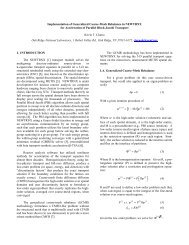
Figure 1shows the plot of the residual directions of the measurements for the case when<br />
there is a bias fault in the narrow range SG level sensor. Note that the NR direction<br />
signature has a maximum value (≈0.9). The direction signatures for the steam flow and<br />
feed flow are not insignificant, primarily because their settings change because of error in<br />
the NR sensor and the resulting feedback. Note that each of the fault direction plots<br />
illustrates nine steady-state operating conditions.<br />
7
Figure 1. Narrow range SG water level sensor bias fault for the case of steady-state plant<br />
operation. The residual directional features are plotted for six different measurements at nine<br />
operating levels. The confidence level for the NR fault has the largest value.<br />
8
An example of tracking turbine control valve fault during transient power operation is<br />
shown in Figure 2. A change in the actuator time constant has been simulated. Figure 2a<br />
is a plot of the measured and model-predicted values of the TCV position. The residual<br />
between the two variables is plotted in Figure 2b. The application illustrates that the<br />
time-dependent GMDH model is able to track the valve error during the transient<br />
operation.<br />
(a) (b)<br />
Figure 2. A comparison of the measured and predicted values of the TCV position is made in<br />
(a).This is the case of fault detection during a plant transient. The residual plot is shown in (b).<br />
The last example illustrates the application of ANFIS modeling and the multi-model<br />
digraph for isolating both single and dual faults. The single fault considered is the feed<br />
water flow transmitter error. The dual fault considers simultaneous errors in the SG<br />
pressure transmitter and the feed water flow transmitter.<br />
Figure 3 shows the plots of feed water flow measurement residual. Among other signals<br />
the model uses the SG pressure. The residual magnitude exceeds the acceptable limit,<br />
indicating a possible fault in the feed water flow transmitter. The model predictions<br />
using the SG pressure and using the reconstructed SG pressure are the same, thus<br />
indicating that the SG pressure is not in error. In the case when the SG pressure<br />
transmitter has an error, the two prediction residuals do not match, as shown in Figure 3b.<br />
This indicates that the SG pressure transmitter is also faulty, in addition to the faulty feed<br />
water flow sensor. The model-based directional graph is able to detect both single and<br />
dual faults.<br />
9
Residual of feed water flow rate<br />
x 10-3<br />
2<br />
0<br />
-2<br />
-4<br />
-6<br />
-8<br />
-10<br />
0 10 20 30 40 50 60 70 80 90-0.025<br />
0 10 20 30 40 50 60 70 80 90<br />
ATTACHMENTS<br />
The following attachments are included<br />
Residual of Feed Water Flow Rate<br />
Sample Number<br />
Attachment I Task 2 Phase 1 Report<br />
Attachment II Task 2 Phase 2 Report<br />
Attachment III Task 2 Phase 3 Report<br />
10<br />
0.005<br />
0<br />
-0.005<br />
-0.01<br />
-0.015<br />
(a) (b)<br />
-----after SG pressure is reconstructed<br />
-0.02<br />
___before SG pressure is reconstructed<br />
Sample Number<br />
Figure 3. Figure 3. Prediction residual of feed water flow transmitter using measured and<br />
reconstructed SG pressure for the case of single fault (a) and simultaneous dual faults (b).
Attachment I<br />
Task 2 Phase 1 Report
Task 2. Phase 1<br />
Advanced Monitoring and Diagnostics<br />
SUMMARY<br />
This report describes the tasks performed and the progress made by The University<br />
of Tennessee (UTK) during 1999-2000 on the DOE-NERI project entitled Automatic<br />
Development of Highly Reliable Control Architecture for Future Nuclear Power<br />
Plants. UTK is collaborating with the Instrumentation & Controls Division of ORNL (lead<br />
organization) and the North Carolina State University (NCSU). The objective of the UTK<br />
research task is to develop an on-line monitoring system for fault detection and isolation<br />
(FDI) of sensors and field devices in a nuclear power plant. In this research emphasis is<br />
given to process instrumentation in a nuclear power plant such as temperature, pressure,<br />
flow, level transmitters, and measurements of control functions. Field devices include<br />
valve actuators, control modules, spray and heater systems, pumps, and other similar<br />
equipment. The goal of this task is to provide diagnostics information to a system<br />
executive for enhanced decision-making by the plant control system.<br />
The following R&D tasks have been accomplished during this reporting period:<br />
• Development of data-driven models for the characterization of sub-system<br />
dynamics for predicting state variables, control functions, and expected control<br />
actions.<br />
• Development of a nonlinear system modeling approach called the Group Method of<br />
Data Handling (GMDH) with rational functions.<br />
• Development of the Principal Component Analysis (PCA) approach for mapping<br />
system measurements.<br />
• Development of a fault detection and isolation module that combines system<br />
operational knowledge (including system simulation) and a rule-based logic for<br />
both single and dual faults in dissimilar sensor and field devices.<br />
• Development of a complimentary approach that quantifies the prediction errors<br />
using a fault pattern classification technique.<br />
The above techniques have been applied to a laboratory process control loop using both<br />
simulation and actual loop measurements. The techniques have been demonstrated for<br />
detecting and isolating faults in sensors and devices in a U-tube steam generator (UTSG) in<br />
a pressurized water reactor (PWR). Only simulation data were used in the latter case.<br />
During the second phase of this project (FY 2000), the FDI system will be<br />
implemented for a UTSG system as part of a full-scope PWR plant being developed by<br />
NCSU. The current methods will be further developed and extended to fault detection<br />
during plant transients. This phase will also include the development of minimum<br />
requirements for application to an existing PWR, and the limitations imposed by the<br />
measurements. The information generated by the FDI module will be interfaced with the<br />
system executive and the control design system. A paper was presented at the American<br />
2
Nuclear Society Annual Meeting, June 2000, and another paper will be presented at the<br />
ANS Topical Meeting on NPIC&HMIT, November 2000.<br />
3
1. INTRODUCTION<br />
1.1 Background and Motivation<br />
Existing and new generation of nuclear power plants have economic and reliability<br />
concerns as addressed by overall plant performance, unscheduled downtime and the longterm<br />
management of critical assets. The key to achieving these needs is to develop an<br />
integrated approach for monitoring, control, fault detection and diagnosis of plant<br />
components such as sensors, actuators, control devices and other equipment. Several<br />
methods developed by industry and academia, for monitoring isolated sensors and system<br />
components were reported [1-8]. Model-based local sensor validation and fault diagnosis<br />
methods were developed for specific applications [3,8]. These approaches assume that a<br />
system fault being monitored occurs in a specific plant component and in an isolated<br />
fashion. Fault detection and isolation (FDI) of sensors and field devices is an important<br />
step towards the implementation of an automated and intelligent process control strategy<br />
[12].<br />
A large-scale system, such as a nuclear power plant, has several feedback control loops.<br />
This makes the identification and isolation of faults in these interconnected systems highly<br />
complex. Even when a sensor used for set point control is faulty, the control system<br />
through feedback, tries to vary the actuating signals until the error in the set point is<br />
eliminated. The sensor-alone type validation will fail in this situation. It is therefore<br />
necessary to consider fault detection and isolation at the system level rather than at the<br />
device level. The objective of this R&D task is to develop an on-line sensor and field<br />
device monitoring and fault detection system, when simultaneous faults may occur in two<br />
or more of these devices. This goal will be achieved by a two-step approach: (1)<br />
Development of data-driven models for predicting multiple variables, using rational<br />
function approximation and group method of data handling; (2) A decision-making module<br />
that uses system functional knowledge base and pattern classification algorithms, that will<br />
be deployed in a distributed configuration. High priority will be given to the<br />
computational efficiency of these techniques, with the capability to change the module<br />
structure with changing plant conditions. The intrinsic merit of the project lies in the<br />
development of an autonomous global monitoring and fault detection approach that would<br />
be executed with minimal human interaction.<br />
1.2 Objectives of R&D and Definition of Tasks<br />
The objective of this research task is to develop an on-line monitoring system for<br />
fault detection and isolation of sensors and field devices in a nuclear power plant. The<br />
sensor suite consists of major process variables in a plant, such as temperature, pressure,<br />
flow, level, and control functions. Field devices in a power plant include, but are not<br />
limited to, valve actuators, control modules, spray and heater systems, pumps, and similar<br />
equipment. The objectives of this R&D are being accomplished through the completion of<br />
the following technical tasks:<br />
• Review of literature and previous work.<br />
4
• Characterization of sub-system dynamics using data-driven models for predicting<br />
state variables, control functions, and expected control actions.<br />
• Development of a Group Method of Data Handling (GMDH) modeling algorithm<br />
with rational function approximation.<br />
• Development of a Principal Component Analysis (PCA) algorithm with linear and<br />
nonlinear mapping.<br />
• Development of an FDI module that combines system operational knowledge and a<br />
rule-based logic for both single and dual faults in dissimilar sensors and field<br />
devices.<br />
• Development of a complimentary module that quantifies the prediction error using a<br />
fault pattern classification technique.<br />
• Demonstration of the FDI system with application to an experimental process<br />
control loop.<br />
• Demonstration of the FDI system with application to a U-tube steam generator<br />
(UTSG) in a full-scope simulation model of a 1,300 MWe PWR.<br />
• Development of minimum requirements for FDI system implementation.<br />
• Extension of the techniques for the case of fault detection during plant transients.<br />
• Identification of realistic faults in a PWR and establish the characteristics of<br />
transient faults as compared with steady-state faults.<br />
• Interfacing the FDI module with control system module via the system executive<br />
and development of a graphical user interface (GUI) for the FDI system<br />
demonstration.<br />
• Identification of issues in technology transfer to nuclear power industry.<br />
• Deliverables: Annual Reports and a Final Report.<br />
FDI software system and User’s Manual.<br />
Conference and journal manuscripts.<br />
1.3 Summary of Significant Accomplishments During 1999-2000<br />
The following major milestones were accomplished during this reporting period:<br />
• Development and testing of the GMDH modeling module for state and control function<br />
prediction.<br />
• Development and testing of the PCA mapping method for system modeling.<br />
• Development and testing of the FDI module for both single and dual/simultaneous<br />
faults.<br />
• Rule-based decision making.<br />
• Fault pattern clustering approach.<br />
• Demonstration of the GMDH method using single and dual faults in a laboratory<br />
process control loop.<br />
• Demonstration of the PCA approach with application to a PWR steam generator<br />
(UTSG) system.<br />
• Preparation of the following manuscripts for publication.<br />
5
• Detection and Isolation of Multiple Faults in Nuclear Plant Systems, ANS<br />
Annual Meeting, San Diego, June 2000.<br />
• Fault Detection and Isolation of Nuclear Power Plant Sensors and Field<br />
Devices, ANS Topical Meeting on NPIC & HMIT, November 2000.<br />
1.4 FDI Architecture and Issues in Developing a Robust FDI Algorithm<br />
Figure 1.1 shows the functional modules of the FDI system being developed in this project.<br />
Both GMDH and PCA modeling of process measurements are considered. This provides a<br />
crosschecking of prediction techniques applied to the measurements. Fault isolation is<br />
based on either a rule-based algorithm or a pattern classification algorithm. The following<br />
issues must be considered in developing a robust FDI algorithm.<br />
• Sensor faults may not be detected in a closed-loop control system.<br />
• Redundancies in sensors and controllers are used in nuclear power plants (NPPs).<br />
• Separation of process variations from sensor/field-device faults must be considered.<br />
• Noise levels in measurements can increase false alarms. It may be necessary to preprocess<br />
signals to eliminate this effect at different sub-bands.<br />
• The use of physics models and data-driven models to understand and characterize the<br />
process dynamics.<br />
1.4 Organization of the Report<br />
The group method of data handling (GMDH) algorithm is described in Section 2 and the<br />
principal component analysis (PCA) is discussed in Section 3. The application of GMDH<br />
to the fault detection and isolation of multiple faults in an experimental process control<br />
loop is presented in Sections 4. Section 5 describes the application of PCA and pattern<br />
classification approach to a U-tube steam generator in a PWR. Concluding remarks and<br />
plans for Phase 2 are given in Section 6.<br />
6
PLANT<br />
DATA-DRIVEN<br />
SYSTEM MODELS<br />
GMDH/PCA<br />
FAULT<br />
DETECTION<br />
OPERATOR<br />
INTERFACE<br />
Figure 1.1. Schematic showing FDI system functional modules.<br />
7<br />
FAULT<br />
ISOLATION
2. GROUP METHOD OF DATA HANDLING (GMDH) APPROACH<br />
FOR MEASUREMENT CHARACTERIZATION<br />
2.1 The GMDH Method with Rational Function Approximation<br />
The objective of this sub-task is to characterize the mapping among process<br />
variables and control functions using self-organizing and data-driven modeling. The socalled<br />
Group Method of Data Handling (GMDH) is an algebraic method for predicting<br />
system states, controller and actuator functions. A new algorithm, that will create<br />
appropriate prediction models for different nuclear plant sub-systems, will be developed<br />
by a rational function approximation of the original GMDH algorithm [11,12]. The GMDH<br />
approach has the advantage over artificial neural networks in not requiring tedious network<br />
training procedures. It is also easy to update the prediction models during plant operation.<br />
The GMDH constructs a model, of a desired output as a function of a set of related<br />
inputs from a subsystem, by a successive polynomial approximation. The general<br />
relationship has the form shown in Equation (2.1) where {x1, x2, … , xm} is a vector of<br />
input variables and y is the variable to be predicted. This formulation can be extended to<br />
the prediction of multiple outputs {y1, y2, … , yn} as well.<br />
m<br />
∑<br />
i=<br />
1<br />
m<br />
m<br />
∑∑<br />
i=<br />
1 j=<br />
1<br />
8<br />
m<br />
m<br />
∑∑∑<br />
y = a + b x + c x x + d x x x + L (2.1)<br />
i<br />
i<br />
ij<br />
i<br />
j<br />
m<br />
i = 1 j=<br />
1 k=<br />
1<br />
A typical node of a GMDH modeling layer is a basic quadratic predictor using variables<br />
[xi, xj]. The model parameters such as {A, B, C, D, E, F}, are estimated from a leastsquares<br />
fit using N observations of the input and output variables.<br />
y = A + Bx + Cx + Dx + Ex + Fx x<br />
i<br />
j<br />
2<br />
i<br />
2<br />
j<br />
i<br />
j<br />
ijk<br />
i<br />
j<br />
k<br />
(2.2)<br />
Figure 2.1 illustrates that the predicted values of y are propagated to successively<br />
higher layers of the algorithm, with the approximation of ypred improving at successive<br />
stages. At each stage of the approximation, ypred is formed from pairs of input signals (to<br />
that layer), and new values of the predicted variable are propagated pair-wise to the next<br />
layer. The iteration is continued until the mean-squared error between the predicted and<br />
the measured values of the output variable attains a desired value.<br />
Parsimony in model fitting is achieved by comparing the fractional prediction<br />
errors from one generation to the next, and by terminating the algorithm when the error is a<br />
minimum or when the difference between errors from successive approximation stages is<br />
less than a preset limit [12].<br />
The GMDH approach described above uses polynomial approximation. This<br />
polynomial set may be satisfactory in establishing some of the relationships of interest. In<br />
characterizing the subsystems in a nuclear power plant it may be necessary to use terms<br />
containing rational functions (for example, ratios of polynomials in x1 and x2). The
expression (2.3) represents a set of such terms that forms a complete set of terms in a given<br />
domain.<br />
⎧<br />
⎪1,<br />
( x1,<br />
x<br />
⎪<br />
⎨<br />
⎪ x1<br />
(<br />
⎪⎩<br />
x1<br />
+ x<br />
2<br />
2<br />
), ( x<br />
x 2 ,<br />
x + x<br />
1<br />
2<br />
1<br />
, x<br />
2<br />
2<br />
2<br />
), ( x<br />
1<br />
x<br />
), (<br />
x<br />
1<br />
2<br />
), (<br />
+ x<br />
x<br />
1<br />
2<br />
1<br />
x<br />
1<br />
,<br />
x<br />
,<br />
1<br />
1<br />
x<br />
2<br />
), (<br />
+ x<br />
x<br />
2<br />
2<br />
1 1 1<br />
, ), (<br />
2 2<br />
x x x + x<br />
1<br />
),...<br />
9<br />
2<br />
1<br />
2<br />
1<br />
,<br />
x x<br />
1<br />
2<br />
), (<br />
x<br />
x<br />
1<br />
2<br />
x<br />
,<br />
x<br />
2<br />
1<br />
⎫<br />
),<br />
⎪<br />
⎬<br />
⎪<br />
⎪⎭<br />
(2.3)<br />
The new set should facilitate the development of prediction models with a<br />
minimum number of terms. The computational efficiency of establishing these models will<br />
be enhanced by a systematic choice of the terms in the set shown in Expression (2.3).<br />
Figure 2.1. GMDH network showing m inputs and K layers.
2.2 The GMDH Algorithm<br />
The following steps explain the procedure used in developing data-driven models<br />
using the group method of data handling.<br />
• Consider N observations of m variables X ≡ {x1, x2, … , xm} and the measurements<br />
of the variable to be estimated, Y ≡ {y1, y2, … , yN}.<br />
• Divide the data into a training set (nt) and a test set (N-nt).<br />
• For each pair {xi, xj} and Y, compute the regression polynomial<br />
y = A + Bx + Cx + Dx + Ex +<br />
i<br />
A total of m(m-1)/2 polynomials are computed.<br />
j<br />
• Create new observations, Z, for each of the new m(m-1)/2 variables.<br />
• Screening out the least effective variables: Compute the SSE<br />
r<br />
2<br />
i<br />
10<br />
2<br />
j<br />
Fx<br />
( y − z )<br />
2<br />
j =<br />
nt<br />
∑<br />
i = 1<br />
i<br />
nt<br />
∑<br />
i = 1<br />
2<br />
y i<br />
ij<br />
2<br />
(2.4)<br />
• Pick those new inputs for which rj < R (choice of the user).<br />
• Repeat the stage-wise computation until the method starts over-fitting the data. Plot<br />
the smallest of {rj} at each stage and look for a minimum. This is called the<br />
minimum Ivakhnenko polynomial.<br />
• Using the best-fit model, compute the prediction errors using the test data of length<br />
(N-nt). Check if the error rbest is satisfactory.<br />
2.3 Enhancement of the GMDH Algorithm<br />
To improve model building with a minimum number of layers, the set of terms<br />
in the regression model is generalized to include rational functions of {x1, x2, … , xm}.<br />
• The choice of terms in the regression is made according to a binary selector:<br />
For example, for k=8, the binary number is between 0 and 255 (a total 256<br />
input vectors).<br />
i<br />
x<br />
j
• Example: model number 179 has the terms [1 0 1 1 0 0 1 1]<br />
• Choose ~ ten best-fit models. From this set, choose the model with the least<br />
number of terms!<br />
• To avoid unlimited increase in the number of nodes in a higher GMDH layer,<br />
use the best m nodes for the succeeding layer. All layers have the same<br />
number of nodes, m.<br />
• Make sure that the number of input variables in the first layer is m > 2, in<br />
order to avoid the termination of GMDH after the first (input) layer.<br />
• To avoid long training times, limit the maximum number of layers for a single<br />
model (30 was suggested in this study, since no improvement was observed<br />
beyond this level).<br />
2.4 Application of the GMDH Algorithm in an FDI System<br />
The choice of the measurement set {x1, x2 , … , xm}, for each predictor y, is<br />
determined from the knowledge of the system, simulation studies, and parametric<br />
analysis such as pair-wise correlations.<br />
• Generate the prediction models using the fault-free data.<br />
• Computes the residual errors for all the state and control functions of interest.<br />
• When the error exceeds a pre-set threshold, a fault is detected.<br />
• Isolate single/multiple faults.<br />
11
3. PRINCIPAL COMPONENT ANALYSIS (PCA) FOR<br />
MEASUREMENT CHARACTERIZATION<br />
3.1 Introduction to Principal Component Analysis (PCA)<br />
Principal Component Analysis (PCA) is a data characterization method that<br />
extracts the directions of maximum variability in a data matrix X (also the matrix of<br />
measurements of process signals). PCA is similar to fitting a hyper-plane in the<br />
measurement space for the normal operation data, and uses a matrix decomposition method.<br />
In case of redundancy in X, the first few principal components (PCs) may be sufficient to<br />
explain most of the variability in the data. The data may then be represented as the<br />
projection on to the sub-space of the retained PCs with minimal loss of information. The<br />
squared sum of errors (SSE) the perpendicular distance of the test data from the PC hyperplane,<br />
and should be small for normal operation (see Figure 3.1). Fault detection is<br />
performed by evaluating the SSE (or residuals) after projecting the test data on to the PC<br />
hyper-plane. A large value of SSE indicates a possible fault in the system.<br />
PCA uses a fundamental result of linear algebra, called the Singular Value<br />
Decomposition (SVD). The following references are suggested [13, 16-23, 25-33, 39].<br />
Singular Value Decomposition (SVD)<br />
SVD: Every (N x m) matrix A can be decomposed into A = U Σ V T , where U and V are<br />
orthogonal matrices, and Σ is diagonal.<br />
A = U S V T = [u1 .. ur .. uN]. Diag[s 1 .. s r]. [v1 .. vr .. vm] T (3.1)<br />
• U(NxN) and V(mxm) are orthogonal matrices: U T U = V T V =I.<br />
• The matrix Σ has the singular values σ1, ... , σr on its diagonal and zero elsewhere.<br />
The dimension r < N and r < m.<br />
Remark:<br />
The singular values {σi} are not eigenvalues of A. But {σi 2 } are eigenvalues of A T A.<br />
Definitions:<br />
A (Nxm) is a rectangular matrix. Its row space (each row has m elements) is r-dimensional<br />
(inside R m ) and its column space (each column has N elements) is r-dimensional (inside<br />
R N ).<br />
12
• Required to choose orthonormal bases: Row space basis: [v1, … , vr] and<br />
column space basis: [u1, … , ur].<br />
We want orthonormal bases that also diagonalize A.<br />
• For a (2x2) matrix A<br />
A[v1 v2] = [σ1u1 σ2u2] = [u1 u2] σ1<br />
AV = UΣ and U T U = V T V =I<br />
• The singular value decomposition (SVD) of A is given by<br />
A = USV -1 = USV T , S is diagonal (*)<br />
• From (*)<br />
σ2<br />
A T A = (UΣV T ) T (UΣV T ) = VΣ T U T UΣV T<br />
A T A = VΣ T ΣV T<br />
• For the symmetric matrix A T A, the columns of V are its eigenvectors corresponding to<br />
its eigenvalues {σ1 2 , ... , σr 2 }. This indicates how to calculate the matrix V.<br />
• Once {vi} are known, the {ui} are calculated from the equations<br />
Avi = σiui, i = 1, 2, … , r<br />
• Remark:<br />
• The vectors {ui} can be calculated directly from AA T .<br />
• AA T = (UΣV T ) (VΣ T U T ) = UΣΣ T U T .<br />
• The columns of U are the eigenvectors of AA T (and correspond to the same eigenvalues<br />
as those of A T A).<br />
• Example:<br />
A = 2 2 A T A = 5 3<br />
-1 1 3 5<br />
13
• Eigenvalues of A T A are σ1 2 =2, σ2 2 =8<br />
• v1 = [-1/2 1/√2 ] t and v2 = [1/√2 1/√2 ] t<br />
• By computing the normalized values of Av1 and Av2, we get<br />
• u1 = [0 1] and u2 = [ 1 0]<br />
• Now verify the results<br />
A = UΣV T = 0 1 √2 0 -1/√2 1/√2<br />
1 0 0 2√2 1/√2 1/√2<br />
Remarks:<br />
The matrices U and V contain orthonormal basis for all four fundamental subspaces:<br />
• First r columns of V: row space of A<br />
• Last m-r columns of V: null space of A<br />
• First r columns of U: column space of A<br />
• Last N-r columns of U: null space of A T<br />
3.3 Principal Component Analysis of Process Data<br />
Consider a data matrix X (N x m) with m variables and N independent measurements.<br />
X = x11 … x1m<br />
x21 … x2m (3.2)<br />
N<br />
xN1 … xNm<br />
m<br />
Decompose X into a product of scores (T) and loadings (P) as<br />
X = TP T + E (3.3)<br />
Where E represents the residuals (error) after projection on to the principal axes or<br />
the hyper-plane. The PCs are ordered such that the successive PCs explain the contribution<br />
to X in descending order of the lengths of principal axes of the hyperellipsoid of the data<br />
space.<br />
Now consider the SVD of the data matrix X:<br />
14
X = USV T (3.4)<br />
• Where<br />
U is an orthogonal matrix (NxN) spanning the column space of X.<br />
V is an orthogonal matrix spanning the row space of X.<br />
S is a diagonal matrix of singular values of X in decreasing magnitude.<br />
Interpretation of the PCA of Process Data<br />
Consider a column vector b (mx1) in the row space of X so that<br />
Xb = US(V T b)<br />
The term in the parentheses represents a rotation of the reference from unit circle to<br />
V.<br />
• Multiplication by S corresponds to a scaling of vector b in the V frame by the<br />
corresponding singular values and transforms b to the column space of X.<br />
• The final vector is in the U-frame and multiplication by U transforms to the<br />
unit hyper sphere in R N .<br />
• The columns of V are the principal components or directions and the singular<br />
values are the lengths of the principal axes of the hyper-ellipsoid.<br />
• The scores T are the projections on to the PCs and are obtained as<br />
• The scores are decorrelated<br />
T = XV = USV T V = US<br />
T T T = (US) T US = S T U T US = S T S<br />
• PCA thus represents a rotation of the Imxm reference frame to the PC<br />
reference frame, so that the data is uncorrelated in the PC frame.<br />
• Retaining p of a maximum rank (X) PCs, the data matrix may be written as<br />
(3.5)<br />
X = UpS pVp T + E<br />
• For a test sample vector x (mx1), the scores (t) and the errors (e) are given by<br />
t = xVp (3.6)<br />
15
(3.7)<br />
e = x – tVp T = x – xVpVp T = x(I-VpVp T )<br />
• The fault vector for each case may then be generated from the error vector e.<br />
The principal component analysis described above performs a linear<br />
transformation of the signals. The PCA may be generalized so that the data matrix X<br />
would consist of nonlinear terms in the measurements. This generalization is<br />
somewhat similar to the use of rational functions in GMDH and is described in Section<br />
2.<br />
16
x 2<br />
20<br />
15<br />
10<br />
5<br />
0<br />
-5<br />
-10<br />
-15<br />
PC 2<br />
-20<br />
-20 -10 0 10 20<br />
x<br />
1<br />
Figure 3.1. Illustration of the principal component analysis (PCA) for a two-dimensional<br />
measurement system.<br />
17<br />
PC 1
4. APPLICATION OF GMDH AND RULE-BASED APPROACH FOR<br />
FAULT DETECTION AND ISOLATION IN A PROCESS CONTROL<br />
LOOP<br />
4.1 Introduction<br />
This section describes the results of the application of the GMDH model prediction<br />
method and a rule-based approach for fault detection and isolation in a laboratory process<br />
control loop. Both single and dual faults were imposed on various devices in this loop. A<br />
description of the experimental facility (along with the sensors and devices used) and<br />
results of loop response simulation are also presented.<br />
The following are the steps in implementing the FDI algorithm:<br />
1. Generation of a fault-free database. Various system operational conditions must be<br />
considered here.<br />
2. Determination of a qualitative relationship among different loop components through<br />
linear correlation analysis.<br />
3. Determination of quantitative relationships among different loop components through<br />
the GMDH technique.<br />
4. Development of a rule-based decision module for fault detection and isolation. This<br />
is accomplished by simulating and characterizing a defined fault in each loop<br />
component.<br />
4.2 GMDH Models and Rational Function Approximation for State and<br />
Control Function Prediction<br />
The Group Method of Data Handling (GMDH) is an algebraic method for<br />
predicting system states, controller and actuator functions. This is described in Section 2.<br />
The GMDH constructs a model, of a desired output as a function of a set of related inputs<br />
from a subsystem, by a successive polynomial approximation. The general relationship has<br />
the form shown in Equation (4.1) where {x1, x2,…,xm} is a vector of input variables and y<br />
is the variable to be predicted. This formulation can be extended to the prediction of<br />
multiple outputs {y1, y2, … , yn}.<br />
m<br />
∑<br />
i=<br />
1<br />
m<br />
m<br />
∑∑<br />
i=<br />
1 j=<br />
1<br />
18<br />
m<br />
m<br />
∑∑∑<br />
y = a + b x + c x x + d x x x + L (4.1)<br />
i<br />
i<br />
ij<br />
i<br />
j<br />
m<br />
i = 1 j=<br />
1 k=<br />
1<br />
Figure 4.1 shows a typical node of a GMDH modeling layer with the basic<br />
quadratic predictor. The model parameters such as {A, B, C, D, E, F}, are estimated from<br />
a least-squares fit using N observations of the input and output variables.<br />
ijk<br />
i<br />
j<br />
k
Figure 4.1. A node of the GMDH model predictor. This node uses a second<br />
order polynomial transfer function.<br />
In application to nuclear plant subsystems, a systematic study has to be performed<br />
in establishing models that are valid for a range of operating conditions. The level of<br />
complexity of the fault detection and identification algorithm depends on the importance of<br />
the equipment or the asset being considered, the ease of real-time monitoring and<br />
communication, and the multiplicity of devices.<br />
4.3 Development of a Mathematical Model of the Laboratory Process<br />
Control System<br />
Theoretical and experimental studies were performed for feasibility studies of the Fault<br />
Detection and Isolation (FDI) method proposed in this work. For the theoretical study, a<br />
simulation model of a process control loop, including sensors, controllers, and actuators,<br />
was developed. This model was implemented in the Matlab-Simulink TM programming<br />
environment. For experimental studies a low-pressure water loop (LPWL) system was<br />
designed and built in the Nuclear Engineering Department [12]. A LabView program was<br />
developed to acquire loop measurements and to control the experiment. Known faults were<br />
imposed on different devices, such as pressure transmitters, motor-operated valves, and<br />
control elements. The purpose of the model and the test system was to provide useful data<br />
and an environment for developing and testing the proposed FDI algorithm. Data from all<br />
available sensors for normal loop operation were used to build a database.<br />
19
The fault detection and isolation system is first tested using a Simulink model of a<br />
process control loop. The control loop is shown in Figure 4.2 and consists of the<br />
following major components: orifice flow meter (RMT flow meter), water level sensor<br />
(pressure transmitter), turbine flow meters (two), three motor-operated valves (MOVs)<br />
with valve position signals, main circulating pump, and a software-driven proportionalintegral<br />
controller for the tank water level. Figure 4.3 shows the main screen of the<br />
Simulink model. A list of all system variables available is given in Table 4.1.<br />
Figure 4.2. A schematic of the low-pressure water loop system, showing<br />
the various sensors and field devices.<br />
Simulation models used for the control loop include (1) mass balance of water in<br />
the tank, P-I controller model, and first order sensor models. An example of steady state<br />
process representation is shown for the pump model with the following parameters.<br />
• IFR = Inlet Flow Rate through tank inlet piping.<br />
• BFR = Bypass Flow Rate through bypass valve<br />
• IMOVP = Inlet MOV Position.<br />
• BMOVP = Bypass MOV Position<br />
• PD = Pump Discharge.<br />
20
Figure 4.3. Physical model of the low-pressure process control loop represented by<br />
Matlab-Simulink [12].<br />
Steady-State Pump Model:<br />
IFR<br />
BFR<br />
IMOVP<br />
=<br />
IMOVP + BMOVP<br />
BMOVP<br />
=<br />
IMOVP + BMOVP<br />
21<br />
*<br />
*<br />
PD<br />
PD<br />
Table 4.1. System variables for the process control loop<br />
(4.2)
Variable (measurement)<br />
1 Bypass MOV position Setpoint<br />
2 Inlet MOV position Setpoint<br />
3 Outlet MOV position Setpoint<br />
4 Measured Bypass MOV position<br />
5 Measured Inlet MOV position<br />
6 Measured Outlet MOV position<br />
7 Water Level Setpoint<br />
8 Measured Water Level<br />
9 PID output<br />
10<br />
Tank Water Temperature set point<br />
11 Tank Water Temperature<br />
12 Heater Element PID Controller Action<br />
13 Measured RMT Inlet Flow rate<br />
14 Measured Turbine Inlet Flow rate<br />
15 Measured Turbine Outlet Flow rate<br />
GMDH prediction models were developed directly from the measurements for tank<br />
inlet flow rate, tank outlet flow rate, tank water level, and level controller signal using the<br />
following functional relationships.<br />
• Inlet Flow Rate = f (Bypass MOV position, Inlet MOV position)<br />
• Outlet Flow Rate = f (Tank water level, Outlet MOV position)<br />
• Tank Water Level = f (Inlet flow rate, Outlet MOV position)<br />
• Controller Output = f (Bypass MOV position, Tank water level, Outlet flow rate)<br />
4.4 Types of (Device) Faults Studied in this Research<br />
22<br />
(4.3)<br />
Many types of faults can occur in a process control loop such as sensor faults,<br />
actuator faults, controller faults, pump failure, leaks in piping, etc. This study limits itself<br />
to those faults that can lead to significant error in the GMDH prediction models. Faults are<br />
introduced in one or more devices during the experiments through the computer interface.<br />
The following is a list of single faults (7) and dual faults (21) that are simulated using the<br />
model.
Single Faults:<br />
Water level sensor drift (sensor fault).<br />
Outlet turbine flow meter drift (sensor fault).<br />
Outlet MOV positioning device drift (actuator fault).<br />
Bypass MOV position (actuator fault).<br />
Inlet MOV positioning device drift (actuator fault).<br />
RMT flow meter drift (sensor fault).<br />
Water Level Controller (controller fault).<br />
Multiple Faults (Dual Faults):<br />
Inlet MOV Fault and Water Level Sensor Fault<br />
Inlet MOV Fault and RMT Flow meter Fault<br />
Inlet MOV Fault and Outlet MOV position<br />
Inlet MOV Fault and Bypass MOV Position<br />
Inlet MOV Fault and PID controller Fault<br />
Water Level Sensor Fault and RMT Flow meter Fault<br />
Water Level Sensor Fault and Outlet MOV position<br />
Water Level Sensor Fault and Bypass MOV Position<br />
Water Level Sensor Fault and Outlet Turbine Flow meter<br />
RMT Flow meter Fault and Outlet MOV position<br />
RMT Flow meter Fault and Bypass MOV Position<br />
RMT Flow meter Fault and Outlet Turbine Flow meter<br />
Outlet MOV position Fault and Bypass MOV Position<br />
Outlet MOV position Fault and Outlet Turbine Flow meter<br />
Bypass MOV Position Fault and Outlet Turbine Flow meter<br />
PI controller Fault and Inlet MOV Fault<br />
PI controller Fault and Water Level Sensor Fault<br />
PI controller Fault and RMT Flow meter Fault<br />
PI controller Fault and Outlet MOV position<br />
PI controller Fault and Bypass MOV Position<br />
PI controller Fault and Outlet Turbine Flow meter.<br />
4.5 Implementation of the FDI Algorithm<br />
The basic steps for developing an FDI algorithm are:<br />
• Generation of the Fault-Free Database<br />
• Generating Qualitative Relationships among Loop Components<br />
• Generating Quantitative Relationships among Loop Components<br />
• Development of a Rule-based Decision Module for Fault Detection and Isolation.<br />
23
4.5.1. Generation of the Fault-Free Database<br />
A fault-free database was generated using the theoretical model for different device<br />
configurations. Bypass and Outlet MOV positions were systematically changed one at a<br />
time. Water level set point was also changed. The Inlet MOV being a part of the water<br />
level control system, its position cannot be set manually; its position is set directly by the<br />
water level controller. No faulty devices were allowed in this phase. About 1,235 cases<br />
were simulated and the data generated were stored in a database. This database is used to<br />
obtain both qualitative and quantitative relationships among the loop devices.<br />
4.5.2. Generating Qualitative Relationships Among Loop Components<br />
To obtain a qualitative relationship among the loop components, the correlation coefficient<br />
method was applied. From this analysis, sets of related variables were defined, although<br />
the characterization of these relationships through mathematical expressions is not obtained<br />
in this step.<br />
Even though sometimes a large set of variables with high correlation existed, groups of<br />
small number of variables were selected for modeling using GMDH. The variables<br />
selected in each group were those from the components that are physically close to each<br />
other. For example the bypass and inlet MOV positions determine the flow that goes<br />
through the inlet piping. One could also use the flow rate that goes through the outlet piping<br />
in the above correlation set, however this variable would not bring new information to this<br />
relationship. Creating a small number of models with local variables makes the fault<br />
detection very efficient, that is, it is easy to isolate a faulty component. This efficiency is<br />
reflected in the rule-based expert system. The simpler the expert system, the easier it is to<br />
develop and maintain it.<br />
Four relationships were defined for this particular loop system. With this relationships the<br />
FDI algorithm is be able to isolate basically all possible faults that may happen in that<br />
loop. The relationships are<br />
• Inlet flow rate as a function of bypass and inlet MOV positions.<br />
• Outlet flow rate as a function of tank water level and outlet MOV position.<br />
• Tank water level as a function of inlet flow rate and outlet MOV position.<br />
• Level controller output value as a function of bypass MOV position, tank water level<br />
and outlet flow rate.<br />
4.5.3. Generating Quantitative Relationships Among Loop Components<br />
For characterization of these four relationships through mathematical equations, the GMDH<br />
method was applied to the same fault-free database. A coefficient matrix representing each<br />
model is generated by the GMDH. This matrix is used to obtain the predicted (or<br />
analytical) component value. This predicted value is then later used for fault detection.<br />
The main task of the GMDH algorithm is to find the model that best maps the input/output<br />
set for given basic functions. After finding the best model, a residual value is computed<br />
24
etween the predicted value and the target value. This residual is stored in memory<br />
(RESIDUAL variable). This variable is used later for comparison purposes among all<br />
residuals from other runs. Each run with a different set of basic functions is tagged with a<br />
number stored in a variable called JobCounter. This variable is used later to recover the<br />
best of the GMDH models. The loop runs 2 n times, where n is the number of basic<br />
functions to be tested.<br />
At the end of this process, the variable called RESIDUAL contains the residuals of all<br />
possible combinations of basic functions (2 n ). Using the Matlab function called SORT<br />
([y, index] = sort(residual)) the residuals are sorted from smallest to the highest values in<br />
the variable Y. The INDEX variable contains the JobCounter case numbers associated<br />
with the residuals in Y. Normally the first JobCounter (index(1)) should be used because<br />
it represents the best set of basic functions for the GMDH model structure.<br />
After establishing the mathematical relationship among a set of loop variables, the model<br />
can be used for generating an analytical redundant measurement. This redundant<br />
measurement is the prediction of the GMDH model.<br />
The Fault Detection and Isolation algorithm uses the comparison between the predicted and<br />
measured values of the process variable under study. If the error (residual) between the<br />
predicted and measured values is higher than a pre-defined threshold, the algorithm<br />
assumes that a fault exists. In this case, a second module is executed; namely, the fault<br />
isolation module. This module is based on a rule-based expert system. This expert system<br />
is described in the next section.<br />
As mentioned earlier in this section, the GMDH algorithm uses the fault-free database to<br />
obtain the best model that maps the input variables (independent variable) to the output<br />
variable (dependent variable). The algorithm splits the input data into two sets of data.<br />
The first set is used to find the best model, while the second monitors for model over<br />
fitting. Figure 4.4 is a plot of the training output data along with the value predicted by the<br />
model for the best set of basic functions. Figure 4.5 is a plot of the test data set with the<br />
predicted values. Finally, Figure 4.6 is a plot of the error (in percent) between the<br />
predicted and the expected output results of the best GMDH model for predicting the flow<br />
rate in the tank inlet piping as a function of Bypass and Inlet MOV positions. The plots<br />
indicate that the GMDH maps the input-output variables satisfactorily for both the training<br />
data and the test data. Figures 4.7 through 4.15 show similar analysis for the Outlet Flow<br />
Rate, PID Controller Output and Tank Water Level.<br />
As an example, the RMS error between the measurement and model prediction for the tank<br />
outlet water flow rate is 0.11%.<br />
25
Inlet Water Flow Rate<br />
x 10-3<br />
16<br />
14<br />
12<br />
10<br />
8<br />
6<br />
4<br />
Only Testing Data Is Plotted Here<br />
2<br />
0 20 40 60 80 100 120 140 160 180<br />
Data Point Number<br />
Figure 4.4. The GMDH predicted values (“o”) against the test output values (“x”)<br />
for the Inlet Flow rate as a function of Bypass MOV and Inlet MOV<br />
positions<br />
.<br />
Inlet Water Flow Rate<br />
x 10-3<br />
14<br />
12<br />
10<br />
8<br />
6<br />
4<br />
2<br />
0 50 100 150 200 250 300 350<br />
Data Point Number<br />
26<br />
GMDH Prediction<br />
Training Data<br />
Figure 4.5. The GMDH predicted values (“o”) against the training output<br />
values (“x”) for the Inlet Flow rate as a function of Bypass MOV<br />
and Inlet MOV positions.
Error(%)<br />
Inlet Flow Rate - Percentagem of Error Between Prediction and Training Data<br />
12<br />
10<br />
8<br />
6<br />
4<br />
2<br />
0<br />
0 50 100 150 200 250 300 350<br />
Data Point Number<br />
Figure 4.6. The error (%) between the predicted values and the measurements for the<br />
Inlet Flow rate as a function of Bypass MOV and Inlet MOV positions.<br />
Outlet Water Flow Rate<br />
0.14<br />
0.12<br />
0.1<br />
0.08<br />
0.06<br />
0.04<br />
0.02<br />
Only Testing Data Is Plotted Here<br />
0<br />
0 20 40 60 80 100 120 140 160 180<br />
Data Point Number<br />
Figure 4.7. The GMDH predicted values (“o”) against the test output values (“x”)<br />
for the Outlet Flow rate as a function of Water Level and Outlet<br />
MOV positions.<br />
27
Outlet Water Flow Rate<br />
0.12<br />
0.1<br />
0.08<br />
0.06<br />
0.04<br />
0.02<br />
0<br />
0 50 100 150 200 250 300 350<br />
Data Point Number<br />
28<br />
GMDH Prediction<br />
Training Data<br />
Figure 4.8. The GMDH predicted values (“o”) against the training output<br />
values (“x”) for the Outlet Flow rate as a function of Water Level<br />
and Outlet MOV positions.<br />
Error(%)<br />
Outlet Flow Rate - Percentagem of Error Between Prediction and Training Data<br />
3.5<br />
3<br />
2.5<br />
2<br />
1.5<br />
1<br />
0.5<br />
0<br />
0 50 100 150 200 250 300 350<br />
Data Point Number<br />
Figure 4.9. The error (%) between the predicted values and the measurements for the<br />
Outlet Flow rate as a function of Water Level and Outlet MOV positions.
PID Controller Output<br />
0.9<br />
0.8<br />
0.7<br />
0.6<br />
0.5<br />
0.4<br />
0.3<br />
0.2<br />
0.1<br />
Only Testing Data Is Plotted Here<br />
0<br />
0 20 40 60 80 100 120 140 160 180<br />
Data Point Number<br />
Figure 4.10. The GMDH predicted values (“o”) against the test output values (x)<br />
for the PID Controller Output as a function of Bypass MOV, Water<br />
Level and Outlet flow rate.<br />
PID Controller Output<br />
1<br />
0.9<br />
0.8<br />
0.7<br />
0.6<br />
0.5<br />
0.4<br />
0.3<br />
0.2<br />
0.1<br />
0<br />
0 50 100 150 200 250 300 350<br />
Data Point Number<br />
29<br />
GMDH Prediction<br />
Training Data<br />
Figure 4.11. The GMDH predicted values (“o”) against the training output<br />
values (“x”) for PID Controller Output as a function of Bypass<br />
MOV, Water Level and Outlet flow rate.
10<br />
9<br />
8<br />
7<br />
6<br />
5<br />
4<br />
Error(%) PID Controller Output - Percentagem of Error Between Prediction and Training Data<br />
3<br />
2<br />
1<br />
0<br />
0 50 100 150 200 250 300 350<br />
Data Point Number<br />
Figure 4.12. The error (%) between the predicted values and the measurements for the<br />
level Controller Output as a function of Bypass MOV, Water Level and<br />
Outlet flow rate.<br />
Water Level<br />
0.065<br />
0.06<br />
0.055<br />
0.05<br />
0.045<br />
0.04<br />
0.035<br />
0.03<br />
Only Testing Data Is Plotted Here<br />
0.025<br />
0 20 40 60 80 100 120 140 160 180<br />
Data Point Number<br />
Figure 4.13. The GMDH predicted values (“o”) against the test output values<br />
(x) for the Tank Water Level as a function of Inlet Flow rate and Outlet MOV positions.<br />
30
Water Level<br />
0.065<br />
0.06<br />
0.055<br />
0.05<br />
0.045<br />
0.04<br />
0.035<br />
0.03<br />
0.025<br />
0 50 100 150 200 250 300 350<br />
Data Point Number<br />
31<br />
GMDH Prediction<br />
Training Data<br />
Figure 4.14. The GMDH predicted values (“o”) against the training output<br />
values (“x”) for the Tank Water Level as a function of Inlet<br />
Flow rate and Outlet MOV positions.<br />
Error(%)<br />
Water Level - Percentagem of Error Between Prediction and Training Data<br />
0.8<br />
0.7<br />
0.6<br />
0.5<br />
0.4<br />
0.3<br />
0.2<br />
0.1<br />
0<br />
0 50 100 150 200 250 300 350<br />
Data Point Number<br />
Figure 4.15. The error (%) between the predicted values and the measurements for the<br />
Tank Water Level as a function of Inlet Flow rate and Outlet MOV positions.
4.5.4. Development of the Rule-based Decision Module for Fault Isolation<br />
The simulation data are generated for various steady-state conditions of the tank water<br />
level. GHDH models are then generated for four variables – inlet flow rate, outlet flow<br />
rate, controller output, and water level. The prediction errors (or the residuals) are used to<br />
develop a comprehensive rule base. Table 4.2 summarizes the behavior of the prediction<br />
errors for each of the faults (both single and dual simultaneous faults). A cell with a '+'<br />
sign indicates that the measured value is greater than the predicted value, and conversely<br />
for a cell with a '-' sign. A cell with no entry indicates that the predicted value is within<br />
3% of the measured value. This threshold level is set by the user.<br />
During normal system operation, the predicted values obtained by the GMDH methods are<br />
very close to those obtained by sensor measurements. However, when a fault occurs in<br />
one of the system components, one or more of these analytical redundant values will not<br />
match with their measurements.<br />
During the experiments, the faults mentioned in the previous section were simulated. The<br />
basic type of fault imposed on the loop devices was a drift type. In all the studied fault<br />
cases, the imposed drift was about 10% of the device nominal value. Figure 4.16 shows a<br />
typical fault profile imposed on the tank water level sensor output. The profile is of the<br />
form tanh(x).<br />
The rule-based expert system uses the system behavior characteristics for each simulated<br />
fault. For most of the cases, the system dynamic behavior responds differently for each<br />
loop component fault. For these cases, each multidimensional residual vector (vector<br />
whose components are made of each individually generated residual) is unique. In cases<br />
where there are two or more different faults that produce the same system behavior, other<br />
system variables was supplied to the expert system:<br />
• Water level set point error.<br />
• Outlet MOV position error.<br />
• Bypass MOV position error.<br />
• Inlet MOV position error.<br />
32
24<br />
23<br />
22<br />
21<br />
20<br />
Water Level Sensor Output (in)<br />
19<br />
18<br />
0 5 10 15<br />
Time (min)<br />
Figure 4.16. Imposed fault profile on the tank water level sensor output.<br />
33
Table 4.2. Summary of behavior of residuals for various fault cases.<br />
Qualitative error between GMDH prediction values and the measured<br />
values for Single and Multiple Fault cases<br />
FAULTS<br />
34<br />
Inlet Flow<br />
rate<br />
Outlet Flow<br />
rate<br />
GMDH Predictions<br />
Controller<br />
Output<br />
Inlet MOV Fault + -<br />
Water Level Sensor Fault - +<br />
RMT Flow Meter Fault + -<br />
Outlet MOV position - +<br />
Bypass MOV position + -<br />
Outlet Turbine Flow meter - +<br />
PID Controller Fault<br />
Inlet MOV Fault and Water Level Sensor + - - +<br />
Inlet MOV Fault and RMT Flow meter + - -<br />
Inlet MOV Fault and Outlet MOV position + - - +<br />
Inlet MOV Fault and Bypass MOV Position<br />
Inlet MOV Fault and Outlet Turbine Flow meter + - +<br />
Water Level Sensor and RMT Flow meter + -<br />
Water Level Sensor and Outlet MOV position - +<br />
Water Level Sensor and Bypass MOV Position - - + +<br />
Water Level Sensor and Outlet Turbine Flow meter - + +<br />
RMT Flow meter and Outlet MOV position + - +<br />
RMT Flow meter and Bypass MOV Position + -<br />
RMT Flow meter and Outlet Turbine Flow meter + - + -<br />
Outlet MOV position and Bypass MOV Position - - + +<br />
Outlet MOV position and Outlet Turbine Flow meter - + +<br />
Bypass MOV Position and Outlet Turbine Flow meter - - +<br />
PID controller Fault and Inlet MOV Fault + -<br />
PID controller Fault and Water Level Sensor - +<br />
PID controller Fault and RMT Flow meter + -<br />
PID controller and Outlet MOV position + - +<br />
PID controller and Bypass MOV Position - +<br />
PID controller and Outlet Turbine Flow meter - +<br />
Water<br />
Level<br />
Using the results shown in Table 4.2 and additional measurements, a rule-based<br />
expert system for fault isolation was developed. The rules consist of if-then statements
ased on the characteristic behavior of each pre-defined fault. A complete list of all the<br />
rules, used for both single and dual-fault situations, is given below.<br />
1) IF (Inlet Flow rate Error > Threshold)<br />
AND (Controller Output Error > Threshold)<br />
AND (Bypass MOV Position Error < Threshold)<br />
THEN Loop Faulty Component = Inlet MOV<br />
2) IF (Outlet Flow rate Error > Threshold)<br />
AND (Water Level Error > Threshold)<br />
AND (Outlet MOV Position Error < Threshold)<br />
THEN Loop Faulty Component = Water Level Sensor<br />
3) IF (Inlet Flow rate Error > Threshold)<br />
AND (Water Level Error > Threshold)<br />
THEN Loop Faulty Component = Inlet Flow rate<br />
4) IF (Outlet Flow rate Error > Threshold)<br />
AND (Water Level Error > Threshold)<br />
AND (Outlet MOV Position Error > Threshold)<br />
THEN Loop Faulty Component = Outlet MOV<br />
5) IF (Inlet Flow rate Error > Threshold)<br />
AND (Controller Output Error > Threshold)<br />
AND (Bypass MOV Position Error > Threshold)<br />
THEN Loop Faulty Component = Bypass MOV<br />
6) IF (Outlet Flow rate Error > Threshold)<br />
AND (Controller Output Error > Threshold)<br />
7) IF (Water Level Set point Error > Threshold)<br />
THEN Loop Faulty Component = Outlet Flow meter<br />
THEN Loop Faulty Component = Water Level Controller<br />
8) IF (Inlet Flow rate Error > Threshold)<br />
AND (Outlet Flow rate Error > Threshold)<br />
AND (Controller Output Error > Threshold)<br />
AND (Water Level Error > Threshold)<br />
AND (Inlet MOV Position Error > Threshold)<br />
THEN Loop Faulty Component = Inlet MOV and Water Level sensor<br />
9) IF (Inlet Flow rate Error > Threshold)<br />
AND (Controller Output Error > Threshold)<br />
35
AND (Water Level Error > Threshold)<br />
AND (Inlet MOV Position Error > Threshold)<br />
THEN Loop Faulty Component = Inlet MOV and RMT Flow meter Fault<br />
10) IF (Inlet Flow rate Error > Threshold)<br />
AND (Outlet Flow rate Error > Threshold)<br />
AND (Controller Output Error > Threshold)<br />
AND (Water Level Error > Threshold)<br />
AND (Outlet MOV Position Error > Threshold)<br />
AND (Inlet MOV Position Error > Threshold)<br />
THEN Loop Faulty Component = Inlet MOV and Outlet MOV Position<br />
11) IF (Bypass MOV Position Error > Threshold)<br />
AND (Inlet MOV Position Error > Threshold)<br />
THEN Loop Faulty Component = Inlet MOV and Bypass MOV Position<br />
12) IF (Inlet Flow rate Error > Threshold)<br />
AND (Outlet Flow rate Error > Threshold)<br />
AND (Controller Output Error > Threshold)<br />
AND (Inlet MOV Position Error > Threshold)<br />
THEN Loop Faulty Component = Inlet MOV and Outlet Turbine Flow meter<br />
13) IF (Inlet Flow rate Error > Threshold)<br />
AND (Outlet Flow rate Error > Threshold)<br />
THEN Loop Faulty Component = Water Level sensor and RMT Flow meter<br />
14) IF (Outlet Flow rate Error > Threshold)<br />
AND (Water Level Error > Threshold)<br />
AND (Outlet MOV Position Error > Threshold)<br />
THEN Loop Faulty Component = Water Level sensor and Outlet MOV<br />
15) IF (Inlet Flow rate Error > Threshold)<br />
AND (Outlet Flow rate Error > Threshold)<br />
AND (Controller Output Error > Threshold)<br />
AND (Water Level Error > Threshold)<br />
AND (Bypass MOV Position Error > Threshold)<br />
16) IF (Outlet Flow rate Error > Threshold)<br />
THEN Loop Faulty Component = Water Level sensor and Bypass MOV<br />
36
AND (Controller Output Error > Threshold)<br />
AND (Water Level Error > Threshold)<br />
THEN Loop Faulty Component = Water Level sensor and Outlet Turbine<br />
17) IF (Inlet Flow rate Error > Threshold)<br />
AND (Outlet Flow rate Error > Threshold)<br />
AND (Water Level Error > Threshold)<br />
AND (Outlet MOV Position Error > Threshold)<br />
THEN Loop Faulty Component = RMT Flow meter and Outlet MOV<br />
18) IF (Controller Output Error > Threshold)<br />
AND (Water Level Error > Threshold)<br />
AND (Bypass MOV Position Error > Threshold)<br />
THEN Loop Faulty Component = RMT Flow meter and Bypass MOV<br />
19) IF (Inlet Flow rate Error > Threshold)<br />
AND (Outlet Flow rate Error > Threshold)<br />
AND (Controller Output Error > Threshold)<br />
AND (Water Level Error > Threshold)<br />
THEN Loop Faulty Component = RMT Flow meter and Outlet Turbine<br />
20) IF (Inlet Flow rate Error > Threshold)<br />
AND (Outlet Flow rate Error > Threshold)<br />
AND (Controller Output Error > Threshold)<br />
AND (Water Level Error > Threshold)<br />
AND (Outlet MOV Position Error > Threshold)<br />
AND (Bypass MOV Position Error > Threshold)<br />
THEN Loop Faulty Component = Outlet MOV Position and Bypass MOV<br />
21) IF (Outlet Flow rate Error > Threshold)<br />
AND (Controller Output Error > Threshold)<br />
AND (Water Level Error > Threshold)<br />
AND (Outlet MOV Position Error > Threshold)<br />
THEN Loop Faulty Component = Outlet MOV Position and Outlet<br />
Turbine Flow meter<br />
22) IF (Inlet Flow rate Error > Threshold)<br />
AND (Outlet Flow rate Error > Threshold)<br />
AND (Controller Output Error > Threshold)<br />
AND (Bypass MOV Position Error > Threshold)<br />
37
THEN Loop Faulty Component = Bypass MOV Position and Outlet<br />
Turbine Flow meter<br />
23) IF (Inlet Flow rate Error > Threshold)<br />
AND (Controller Output Error > Threshold)<br />
AND (Water Level Set point Error > Threshold)<br />
AND (Inlet MOV Position Error > Threshold)<br />
THEN Loop Faulty Component = PID Controller and Inlet MOV faults<br />
24) IF (Outlet Flow rate Error > Threshold)<br />
AND (Water Level Error > Threshold)<br />
AND (Water Level Set point Error > Threshold)<br />
THEN Loop Faulty Component = PID Controller and Water Level sensor<br />
25) IF (Inlet Flow rate Error > Threshold)<br />
AND (Water Level Error > Threshold)<br />
AND (Water Level Set point Error > Threshold)<br />
THEN Loop Faulty Component = PID Controller and RMT Flow meter<br />
26) IF (Inlet Flow rate Error > Threshold)<br />
AND (Outlet Flow rate Error > Threshold)<br />
AND (Water Level Error > Threshold)<br />
AND (Water Level Set point Error > Threshold)<br />
AND (Outlet MOV Position Error > Threshold)<br />
Position<br />
THEN Loop Faulty Component = PID Controller and Outlet MOV<br />
27) IF (Inlet Flow rate Error > Threshold)<br />
AND (Controller Output Error > Threshold)<br />
AND (Water Level Set point Error > Threshold)<br />
AND (Bypass MOV Position Error > Threshold)<br />
Position<br />
THEN Loop Faulty Component = PID Controller and Bypass MOV<br />
28) IF (Outlet Flow rate Error > Threshold)<br />
AND (Controller Output Error > Threshold)<br />
AND (Water Level Set point Error > Threshold)<br />
Remarks:<br />
THEN Loop Faulty Component = PID Controller and Outlet Turbine Flow meter<br />
Using the above rules we could detect and isolate single and dual faults occurring<br />
in the experimental water loop, except in one case. This case occurs when we have Outlet<br />
MOV position fault (single fault) or Water Level sensor fault and Outlet MOV position<br />
38
fault (dual fault). In both these cases, the values of the GMDH predictions have similar<br />
behavior. In such cases, additional information or measurements are necessary to resolve<br />
the faulty situation.<br />
4.6 Results of Simulation of Fault Detection and Isolation Studies<br />
The following is a summary of the results of a simulation study of the fault detection and<br />
isolation simulation performed using the Matlab-Simulink model. All the single and<br />
double fault cases were simulated. The results of this study demonstrate that the<br />
performance of the FDI algorithm in detecting faulty sensors/devices is excellent.<br />
Predicted Inlet Flow rate: 0.010424<br />
Model Inlet Flow rate: 0.010346<br />
Percentage of Variation: -0.754702 (%)<br />
Predicted Outlet Flow rate: 0.083300<br />
Model Outlet Flow rate: 0.082766<br />
Percentage of Variation: -0.645251 (%)<br />
Predicted PID Output: 0.493633<br />
Model PID Output: 0.494193<br />
Percentage of Variation: 0.113352 (%)<br />
Predicted Water Level: 0.042740<br />
Model Water Level: 0.042857<br />
Percentage of Variation: 0.273263 (%)<br />
Water Level Setpoint: 0.042857<br />
Measured Water Level: 0.042857<br />
Percentage of Variation: 0.000000 (%)<br />
Outlet MOV Setpoint Position: 0.900000<br />
Measured Position: 0.900000<br />
Percentage of Variation: 0.000000 (%)<br />
Bypass MOV Setpoint Position: 0.700000<br />
Measured Position: 0.700000<br />
Percentage of Variation: 0.000000 (%)<br />
Inlet MOV Setpoint Position: 0.494193<br />
Measured Position: 0.494193<br />
39
Percentage of Variation: 0.000000 (%)<br />
Fault Type =<br />
No fault detected<br />
40
Predicted Inlet Flow rate: 0.009717<br />
Model Inlet Flow rate: 0.010346<br />
Percentage of Variation: 6.081036 (%)<br />
Predicted Outlet Flow rate: 0.083300<br />
Model Outlet Flow rate: 0.082766<br />
Percentage of Variation: -0.645251 (%)<br />
Predicted PID Output: 0.493633<br />
Model PID Output: 0.444940<br />
Percentage of Variation: -10.943678 (%)<br />
Predicted Water Level: 0.042740<br />
Model Water Level: 0.042857<br />
Percentage of Variation: 0.273263 (%)<br />
Water Level Setpoint: 0.042857<br />
Measured Water Level: 0.042857<br />
Percentage of Variation: 0.000000 (%)<br />
Outlet MOV Setpoint Position: 0.900000<br />
Measured Position: 0.900000<br />
Percentage of Variation: 0.000000 (%)<br />
Bypass MOV Setpoint Position: 0.700000<br />
Measured Position: 0.700000<br />
Percentage of Variation: 0.000000 (%)<br />
Inlet MOV Setpoint Position: 0.444940<br />
Measured Position: 0.494193<br />
Percentage of Variation: -11.069578 (%)<br />
Fault Type =<br />
Inlet MOV Fault<br />
41
Process Time: 0.520000<br />
Predicted Inlet Flow rate: 0.009277<br />
Model Inlet Flow rate: 0.009317<br />
Percentage of Variation: 0.434580 (%)<br />
Predicted Outlet Flow rate: 0.083300<br />
Model Outlet Flow rate: 0.074539<br />
Percentage of Variation: -11.753406 (%)<br />
Predicted PID Output: 0.419792<br />
Model PID Output: 0.415886<br />
Percentage of Variation: -0.939251 (%)<br />
Predicted Water Level: 0.038533<br />
Model Water Level: 0.042857<br />
Percentage of Variation: 10.089986 (%)<br />
Water Level Setpoint: 0.042857<br />
Measured Water Level: 0.042857<br />
Percentage of Variation: 0.000000 (%)<br />
Outlet MOV Setpoint Position: 0.900000<br />
Measured Position: 0.900000<br />
Percentage of Variation: 0.000000 (%)<br />
Bypass MOV Setpoint Position: 0.700000<br />
Measured Position: 0.700000<br />
Percentage of Variation: 0.000000 (%)<br />
Inlet MOV Setpoint Position: 0.415886<br />
Measured Position: 0.415886<br />
Percentage of Variation: 0.000000 (%)<br />
Fault Type =<br />
Water Level Sensor Fault<br />
42
Predicted Inlet Flow rate: 0.010424<br />
Model Inlet Flow rate: 0.011396<br />
Percentage of Variation: 8.531987 (%)<br />
Predicted Outlet Flow rate: 0.083300<br />
Model Outlet Flow rate: 0.082766<br />
Percentage of Variation: -0.645251 (%)<br />
Predicted PID Output: 0.493633<br />
Model PID Output: 0.494193<br />
Percentage of Variation: 0.113352 (%)<br />
Predicted Water Level: 0.047109<br />
Model Water Level: 0.042857<br />
Percentage of Variation: -9.921735 (%)<br />
Water Level Setpoint: 0.042857<br />
Measured Water Level: 0.042857<br />
Percentage of Variation: 0.000000 (%)<br />
Outlet MOV Setpoint Position: 0.900000<br />
Measured Position: 0.900000<br />
Percentage of Variation: 0.000000 (%)<br />
Bypass MOV Setpoint Position: 0.700000<br />
Measured Position: 0.700000<br />
Percentage of Variation: 0.000000 (%)<br />
Inlet MOV Setpoint Position: 0.494193<br />
Measured Position: 0.494193<br />
Percentage of Variation: 0.000000 (%)<br />
Fault Type =<br />
RMT Flow meter Fault<br />
43
Predicted Inlet Flow rate: 0.008303<br />
Model Inlet Flow rate: 0.008434<br />
Percentage of Variation: 1.554577 (%)<br />
Predicted Outlet Flow rate: 0.083300<br />
Model Outlet Flow rate: 0.067471<br />
Percentage of Variation: -23.460349 (%)<br />
Predicted PID Output: 0.365378<br />
Model PID Output: 0.356373<br />
Percentage of Variation: -2.526843 (%)<br />
Predicted Water Level: 0.034919<br />
Model Water Level: 0.042857<br />
Percentage of Variation: 18.521490 (%)<br />
Water Level Setpoint: 0.042857<br />
Measured Water Level: 0.042857<br />
Percentage of Variation: 0.000000 (%)<br />
Outlet MOV Setpoint Position: 0.900000<br />
Measured Position: 0.812597<br />
Percentage of Variation: 9.711405 (%)<br />
Bypass MOV Setpoint Position: 0.700000<br />
Measured Position: 0.700000<br />
Percentage of Variation: 0.000000 (%)<br />
Inlet MOV Setpoint Position: 0.356373<br />
Measured Position: 0.356373<br />
Percentage of Variation: 0.000000 (%)<br />
Fault Type =<br />
Outlet MOV Position<br />
44
Predicted Inlet Flow rate: 0.011022<br />
Model Inlet Flow rate: 0.010346<br />
Percentage of Variation: -6.540570 (%)<br />
Predicted Outlet Flow rate: 0.083300<br />
Model Outlet Flow rate: 0.082766<br />
Percentage of Variation: -0.645251 (%)<br />
Predicted PID Output: 0.493633<br />
Model PID Output: 0.544582<br />
Percentage of Variation: 9.355584 (%)<br />
Predicted Water Level: 0.042740<br />
Model Water Level: 0.042857<br />
Percentage of Variation: 0.273263 (%)<br />
Water Level Setpoint: 0.042857<br />
Measured Water Level: 0.042857<br />
Percentage of Variation: 0.000000 (%)<br />
Outlet MOV Setpoint Position: 0.900000<br />
Measured Position: 0.900000<br />
Percentage of Variation: 0.000000 (%)<br />
Bypass MOV Setpoint Position: 0.700000<br />
Measured Position: 0.771373<br />
Percentage of Variation: -10.196140 (%)<br />
Inlet MOV Setpoint Position: 0.544582<br />
Measured Position: 0.544582<br />
Percentage of Variation: 0.000000 (%)<br />
Fault Type =<br />
Bypass MOV Position<br />
45
Predicted Inlet Flow rate: 0.010424<br />
Model Inlet Flow rate: 0.010346<br />
Percentage of Variation: -0.754702 (%)<br />
Predicted Outlet Flow rate: 0.083300<br />
Model Outlet Flow rate: 0.074537<br />
Percentage of Variation: -11.756441 (%)<br />
Predicted PID Output: 0.419776<br />
Model PID Output: 0.494193<br />
Percentage of Variation: 15.058347 (%)<br />
Predicted Water Level: 0.042740<br />
Model Water Level: 0.042857<br />
Percentage of Variation: 0.273263 (%)<br />
Water Level Setpoint: 0.042857<br />
Measured Water Level: 0.042857<br />
Percentage of Variation: 0.000000 (%)<br />
Outlet MOV Setpoint Position: 0.900000<br />
Measured Position: 0.900000<br />
Percentage of Variation: 0.000000 (%)<br />
Bypass MOV Setpoint Position: 0.700000<br />
Measured Position: 0.700000<br />
Percentage of Variation: 0.000000 (%)<br />
Inlet MOV Setpoint Position: 0.494193<br />
Measured Position: 0.494193<br />
Percentage of Variation: 0.000000 (%)<br />
Fault Type =<br />
Outlet Turbine Flow meter<br />
46
Predicted Inlet Flow rate: 0.006892<br />
Model Inlet Flow rate: 0.007089<br />
Percentage of Variation: 2.779387 (%)<br />
Predicted Outlet Flow rate: 0.056598<br />
Model Outlet Flow rate: 0.056690<br />
Percentage of Variation: 0.162781 (%)<br />
Predicted PID Output: 0.293820<br />
Model PID Output: 0.283548<br />
Percentage of Variation: -3.622405 (%)<br />
Predicted Water Level: 0.029344<br />
Model Water Level: 0.029355<br />
Percentage of Variation: 0.037995 (%)<br />
Water Level Setpoint: 0.042857<br />
Measured Water Level: 0.029355<br />
Percentage of Variation: 31.505365 (%)<br />
Outlet MOV Setpoint Position: 0.900000<br />
Measured Position: 0.900000<br />
Percentage of Variation: 0.000000 (%)<br />
Bypass MOV Setpoint Position: 0.700000<br />
Measured Position: 0.700000<br />
Percentage of Variation: 0.000000 (%)<br />
Inlet MOV Setpoint Position: 0.283548<br />
Measured Position: 0.283548<br />
Percentage of Variation: 0.000000 (%)<br />
Fault Type =<br />
PID controller Fault<br />
47
Predicted Inlet Flow rate: 0.008474<br />
Model Inlet Flow rate: 0.009308<br />
Percentage of Variation: 8.955284 (%)<br />
Predicted Outlet Flow rate: 0.083300<br />
Model Outlet Flow rate: 0.074463<br />
Percentage of Variation: -11.867831 (%)<br />
Predicted PID Output: 0.419165<br />
Model PID Output: 0.365631<br />
Percentage of Variation: -14.641400 (%)<br />
Predicted Water Level: 0.038494<br />
Model Water Level: 0.042857<br />
Percentage of Variation: 10.180673 (%)<br />
Water Level Setpoint: 0.042857<br />
Measured Water Level: 0.042857<br />
Percentage of Variation: 0.000000 (%)<br />
Outlet MOV Setpoint Position: 0.900000<br />
Measured Position: 0.900000<br />
Percentage of Variation: 0.000000 (%)<br />
Bypass MOV Setpoint Position: 0.700000<br />
Measured Position: 0.700000<br />
Percentage of Variation: 0.000000 (%)<br />
Inlet MOV Setpoint Position: 0.365631<br />
Measured Position: 0.415208<br />
Percentage of Variation: -13.559418 (%)<br />
Fault Type =<br />
Inlet MOV Fault and Water Level Sensor Fault<br />
48
Predicted Inlet Flow rate: 0.009710<br />
Model Inlet Flow rate: 0.011386<br />
Percentage of Variation: 14.724183 (%)<br />
Predicted Outlet Flow rate: 0.083300<br />
Model Outlet Flow rate: 0.082766<br />
Percentage of Variation: -0.645251 (%)<br />
Predicted PID Output: 0.493633<br />
Model PID Output: 0.444491<br />
Percentage of Variation: -11.055774 (%)<br />
Predicted Water Level: 0.047068<br />
Model Water Level: 0.042857<br />
Percentage of Variation: -9.824562 (%)<br />
Water Level Setpoint: 0.042857<br />
Measured Water Level: 0.042857<br />
Percentage of Variation: 0.000000 (%)<br />
Outlet MOV Setpoint Position: 0.900000<br />
Measured Position: 0.900000<br />
Percentage of Variation: 0.000000 (%)<br />
Bypass MOV Setpoint Position: 0.700000<br />
Measured Position: 0.700000<br />
Percentage of Variation: 0.000000 (%)<br />
Inlet MOV Setpoint Position: 0.444491<br />
Measured Position: 0.494193<br />
Percentage of Variation: -11.181801 (%)<br />
Fault Type =<br />
Inlet MOV Fault and RMT Flow meter Fault<br />
49
Predicted Inlet Flow rate: 0.007382<br />
Model Inlet Flow rate: 0.008439<br />
Percentage of Variation: 12.520947 (%)<br />
Predicted Outlet Flow rate: 0.083300<br />
Model Outlet Flow rate: 0.067509<br />
Percentage of Variation: -23.391954 (%)<br />
Predicted PID Output: 0.365648<br />
Model PID Output: 0.308802<br />
Percentage of Variation: -18.408437 (%)<br />
Predicted Water Level: 0.034939<br />
Model Water Level: 0.042857<br />
Percentage of Variation: 18.476632 (%)<br />
Water Level Setpoint: 0.042857<br />
Measured Water Level: 0.042857<br />
Percentage of Variation: 0.000000 (%)<br />
Outlet MOV Setpoint Position: 0.900000<br />
Measured Position: 0.812823<br />
Percentage of Variation: 9.686386 (%)<br />
Bypass MOV Setpoint Position: 0.700000<br />
Measured Position: 0.700000<br />
Percentage of Variation: 0.000000 (%)<br />
Inlet MOV Setpoint Position: 0.308802<br />
Measured Position: 0.356672<br />
Percentage of Variation: -15.501652 (%)<br />
Fault Type =<br />
Inlet MOV Fault and Outlet MOV Position<br />
50
Predicted Inlet Flow rate: 0.010424<br />
Model Inlet Flow rate: 0.010346<br />
Percentage of Variation: -0.754702 (%)<br />
Predicted Outlet Flow rate: 0.083300<br />
Model Outlet Flow rate: 0.082766<br />
Percentage of Variation: -0.645251 (%)<br />
Predicted PID Output: 0.493633<br />
Model PID Output: 0.494193<br />
Percentage of Variation: 0.113352 (%)<br />
Predicted Water Level: 0.042740<br />
Model Water Level: 0.042857<br />
Percentage of Variation: 0.273263 (%)<br />
Water Level Setpoint: 0.042857<br />
Measured Water Level: 0.042857<br />
Percentage of Variation: 0.000000 (%)<br />
Outlet MOV Setpoint Position: 0.900000<br />
Measured Position: 0.900000<br />
Percentage of Variation: 0.000000 (%)<br />
Bypass MOV Setpoint Position: 0.700000<br />
Measured Position: 0.769764<br />
Percentage of Variation: -9.966345 (%)<br />
Inlet MOV Setpoint Position: 0.494193<br />
Measured Position: 0.543446<br />
Percentage of Variation: -9.966345 (%)<br />
Fault Type =<br />
Inlet MOV Fault and Bypass MOV Position<br />
51
Predicted Inlet Flow rate: 0.009719<br />
Model Inlet Flow rate: 0.010346<br />
Percentage of Variation: 6.061601 (%)<br />
Predicted Outlet Flow rate: 0.083300<br />
Model Outlet Flow rate: 0.074539<br />
Percentage of Variation: -11.753406 (%)<br />
Predicted PID Output: 0.419792<br />
Model PID Output: 0.445071<br />
Percentage of Variation: 5.679639 (%)<br />
Predicted Water Level: 0.042740<br />
Model Water Level: 0.042857<br />
Percentage of Variation: 0.273263 (%)<br />
Water Level Setpoint: 0.042857<br />
Measured Water Level: 0.042857<br />
Percentage of Variation: 0.000000 (%)<br />
Outlet MOV Setpoint Position: 0.900000<br />
Measured Position: 0.900000<br />
Percentage of Variation: 0.000000 (%)<br />
Bypass MOV Setpoint Position: 0.700000<br />
Measured Position: 0.700000<br />
Percentage of Variation: 0.000000 (%)<br />
Inlet MOV Setpoint Position: 0.445071<br />
Measured Position: 0.494193<br />
Percentage of Variation: -11.036939 (%)<br />
Fault Type =<br />
Inlet MOV Fault and Outlet Turbine Flow meter<br />
52
Predicted Inlet Flow rate: 0.009253<br />
Model Inlet Flow rate: 0.010346<br />
Percentage of Variation: 10.557606 (%)<br />
Predicted Outlet Flow rate: 0.083300<br />
Model Outlet Flow rate: 0.074363<br />
Percentage of Variation: -12.018408 (%)<br />
Predicted PID Output: 0.418342<br />
Model PID Output: 0.414320<br />
Percentage of Variation: -0.970680 (%)<br />
Predicted Water Level: 0.042740<br />
Model Water Level: 0.042857<br />
Percentage of Variation: 0.273263 (%)<br />
Water Level Setpoint: 0.042857<br />
Measured Water Level: 0.042857<br />
Percentage of Variation: 0.000000 (%)<br />
Outlet MOV Setpoint Position: 0.900000<br />
Measured Position: 0.900000<br />
Percentage of Variation: 0.000000 (%)<br />
Bypass MOV Setpoint Position: 0.700000<br />
Measured Position: 0.700000<br />
Percentage of Variation: 0.000000 (%)<br />
Inlet MOV Setpoint Position: 0.414320<br />
Measured Position: 0.414320<br />
Percentage of Variation: 0.000000 (%)<br />
Fault Type =<br />
Water Level Sensor Fault and RMT Flow meter Fault<br />
53
Predicted Inlet Flow rate: 0.005767<br />
Model Inlet Flow rate: 0.005879<br />
Percentage of Variation: 1.901189 (%)<br />
Predicted Outlet Flow rate: 0.065678<br />
Model Outlet Flow rate: 0.047030<br />
Percentage of Variation: -39.651459 (%)<br />
Predicted PID Output: 0.248721<br />
Model PID Output: 0.245957<br />
Percentage of Variation: -1.123806 (%)<br />
Predicted Water Level: 0.030823<br />
Model Water Level: 0.042857<br />
Percentage of Variation: 28.079230 (%)<br />
Water Level Setpoint: 0.042857<br />
Measured Water Level: 0.042857<br />
Percentage of Variation: 0.000024 (%)<br />
Outlet MOV Setpoint Position: 0.800000<br />
Measured Position: 0.716747<br />
Percentage of Variation: 10.406626 (%)<br />
Bypass MOV Setpoint Position: 0.800000<br />
Measured Position: 0.800000<br />
Percentage of Variation: 0.000000 (%)<br />
Inlet MOV Setpoint Position: 0.245957<br />
Measured Position: 0.245957<br />
Percentage of Variation: 0.000000 (%)<br />
Fault Type =<br />
Water Level Sensor Fault and Outlet MOV Position<br />
54
Predicted Inlet Flow rate: 0.009888<br />
Model Inlet Flow rate: 0.009290<br />
Percentage of Variation: -6.436993 (%)<br />
Predicted Outlet Flow rate: 0.083300<br />
Model Outlet Flow rate: 0.074316<br />
Percentage of Variation: -12.088435 (%)<br />
Predicted PID Output: 0.417960<br />
Model PID Output: 0.456164<br />
Percentage of Variation: 8.375028 (%)<br />
Predicted Water Level: 0.038419<br />
Model Water Level: 0.042857<br />
Percentage of Variation: 10.354989 (%)<br />
Water Level Setpoint: 0.042857<br />
Measured Water Level: 0.042857<br />
Percentage of Variation: -0.000000 (%)<br />
Outlet MOV Setpoint Position: 0.900000<br />
Measured Position: 0.900000<br />
Percentage of Variation: 0.000000 (%)<br />
Bypass MOV Setpoint Position: 0.700000<br />
Measured Position: 0.771463<br />
Percentage of Variation: -10.209068 (%)<br />
Inlet MOV Setpoint Position: 0.456164<br />
Measured Position: 0.456164<br />
Percentage of Variation: 0.000000 (%)<br />
Fault Type =<br />
Water Level Sensor Fault and Bypass MOV Position<br />
55
Predicted Inlet Flow rate: 0.009270<br />
Model Inlet Flow rate: 0.009310<br />
Percentage of Variation: 0.439513 (%)<br />
Predicted Outlet Flow rate: 0.083300<br />
Model Outlet Flow rate: 0.066202<br />
Percentage of Variation: -25.827818 (%)<br />
Predicted PID Output: 0.356337<br />
Model PID Output: 0.415394<br />
Percentage of Variation: 14.217085 (%)<br />
Predicted Water Level: 0.038505<br />
Model Water Level: 0.042857<br />
Percentage of Variation: 10.155823 (%)<br />
Water Level Setpoint: 0.042857<br />
Measured Water Level: 0.042857<br />
Percentage of Variation: 0.000000 (%)<br />
Outlet MOV Setpoint Position: 0.900000<br />
Measured Position: 0.900000<br />
Percentage of Variation: 0.000000 (%)<br />
Bypass MOV Setpoint Position: 0.700000<br />
Measured Position: 0.700000<br />
Percentage of Variation: 0.000000 (%)<br />
Inlet MOV Setpoint Position: 0.415394<br />
Measured Position: 0.415394<br />
Percentage of Variation: 0.000000 (%)<br />
Fault Type =<br />
Water Level Sensor Fault and Outlet Turbine Flow meter<br />
56
Predicted Inlet Flow rate: 0.008226<br />
Model Inlet Flow rate: 0.009410<br />
Percentage of Variation: 12.578092 (%)<br />
Predicted Outlet Flow rate: 0.083300<br />
Model Outlet Flow rate: 0.066955<br />
Percentage of Variation: -24.412211 (%)<br />
Predicted PID Output: 0.361678<br />
Model PID Output: 0.352275<br />
Percentage of Variation: -2.669276 (%)<br />
Predicted Water Level: 0.038910<br />
Model Water Level: 0.042857<br />
Percentage of Variation: 9.209935 (%)<br />
Water Level Setpoint: 0.042857<br />
Measured Water Level: 0.042857<br />
Percentage of Variation: -0.000000 (%)<br />
Outlet MOV Setpoint Position: 0.900000<br />
Measured Position: 0.809483<br />
Percentage of Variation: 10.057462 (%)<br />
Bypass MOV Setpoint Position: 0.700000<br />
Measured Position: 0.700000<br />
Percentage of Variation: 0.000000 (%)<br />
Inlet MOV Setpoint Position: 0.352275<br />
Measured Position: 0.352275<br />
Percentage of Variation: 0.000000 (%)<br />
Fault Type =<br />
RMT Flow meter Fault and Outlet MOV Position<br />
57
Predicted Inlet Flow rate: 0.011006<br />
Model Inlet Flow rate: 0.011371<br />
Percentage of Variation: 3.216201 (%)<br />
Predicted Outlet Flow rate: 0.083300<br />
Model Outlet Flow rate: 0.082766<br />
Percentage of Variation: -0.645251 (%)<br />
Predicted PID Output: 0.493633<br />
Model PID Output: 0.543179<br />
Percentage of Variation: 9.121466 (%)<br />
Predicted Water Level: 0.047005<br />
Model Water Level: 0.042857<br />
Percentage of Variation: -9.677425 (%)<br />
Water Level Setpoint: 0.042857<br />
Measured Water Level: 0.042857<br />
Percentage of Variation: 0.000000 (%)<br />
Outlet MOV Setpoint Position: 0.900000<br />
Measured Position: 0.900000<br />
Percentage of Variation: 0.000000 (%)<br />
Bypass MOV Setpoint Position: 0.700000<br />
Measured Position: 0.769386<br />
Percentage of Variation: -9.912258 (%)<br />
Inlet MOV Setpoint Position: 0.543179<br />
Measured Position: 0.543179<br />
Percentage of Variation: 0.000000 (%)<br />
Fault Type =<br />
RMT Flow meter Fault and Bypass MOV Position<br />
58
Predicted Inlet Flow rate: 0.010424<br />
Model Inlet Flow rate: 0.011405<br />
Percentage of Variation: 8.604518 (%)<br />
Predicted Outlet Flow rate: 0.083300<br />
Model Outlet Flow rate: 0.074290<br />
Percentage of Variation: -12.127503 (%)<br />
Predicted PID Output: 0.417748<br />
Model PID Output: 0.494193<br />
Percentage of Variation: 15.468661 (%)<br />
Predicted Water Level: 0.047147<br />
Model Water Level: 0.042857<br />
Percentage of Variation: -10.010503 (%)<br />
Water Level Setpoint: 0.042857<br />
Measured Water Level: 0.042857<br />
Percentage of Variation: 0.000000 (%)<br />
Outlet MOV Setpoint Position: 0.900000<br />
Measured Position: 0.900000<br />
Percentage of Variation: 0.000000 (%)<br />
Bypass MOV Setpoint Position: 0.700000<br />
Measured Position: 0.700000<br />
Percentage of Variation: 0.000000 (%)<br />
Inlet MOV Setpoint Position: 0.494193<br />
Measured Position: 0.494193<br />
Percentage of Variation: 0.000000 (%)<br />
Fault Type =<br />
RMT Flow meter Fault and Outlet Turbine Flow meter<br />
59
Predicted Inlet Flow rate: 0.008802<br />
Model Inlet Flow rate: 0.008313<br />
Percentage of Variation: -5.874404 (%)<br />
Predicted Outlet Flow rate: 0.083300<br />
Model Outlet Flow rate: 0.066505<br />
Percentage of Variation: -25.253264 (%)<br />
Predicted PID Output: 0.358482<br />
Model PID Output: 0.384859<br />
Percentage of Variation: 6.853725 (%)<br />
Predicted Water Level: 0.034422<br />
Model Water Level: 0.042857<br />
Percentage of Variation: 19.681264 (%)<br />
Water Level Setpoint: 0.042857<br />
Measured Water Level: 0.042857<br />
Percentage of Variation: -0.000000 (%)<br />
Outlet MOV Setpoint Position: 0.900000<br />
Measured Position: 0.806761<br />
Percentage of Variation: 10.359944 (%)<br />
Bypass MOV Setpoint Position: 0.700000<br />
Measured Position: 0.772520<br />
Percentage of Variation: -10.359944 (%)<br />
Inlet MOV Setpoint Position: 0.384859<br />
Measured Position: 0.384859<br />
Percentage of Variation: 0.000000 (%)<br />
Fault Type =<br />
Outlet MOV position Fault and Bypass MOV Position<br />
60
Predicted Inlet Flow rate: 0.008150<br />
Model Inlet Flow rate: 0.008305<br />
Percentage of Variation: 1.869022 (%)<br />
Predicted Outlet Flow rate: 0.083300<br />
Model Outlet Flow rate: 0.057826<br />
Percentage of Variation: -44.052817 (%)<br />
Predicted PID Output: 0.300900<br />
Model PID Output: 0.348203<br />
Percentage of Variation: 13.584896 (%)<br />
Predicted Water Level: 0.034388<br />
Model Water Level: 0.042857<br />
Percentage of Variation: 19.762091 (%)<br />
Water Level Setpoint: 0.042857<br />
Measured Water Level: 0.042857<br />
Percentage of Variation: -0.000000 (%)<br />
Outlet MOV Setpoint Position: 0.900000<br />
Measured Position: 0.806353<br />
Percentage of Variation: 10.405262 (%)<br />
Bypass MOV Setpoint Position: 0.700000<br />
Measured Position: 0.700000<br />
Percentage of Variation: 0.000000 (%)<br />
Inlet MOV Setpoint Position: 0.348203<br />
Measured Position: 0.348203<br />
Percentage of Variation: 0.000000 (%)<br />
Fault Type =<br />
Outlet MOV Position Fault and Outlet Turbine Flow meter<br />
61
Predicted Inlet Flow rate: 0.011028<br />
Model Inlet Flow rate: 0.010346<br />
Percentage of Variation: -6.591704 (%)<br />
Predicted Outlet Flow rate: 0.083300<br />
Model Outlet Flow rate: 0.074254<br />
Percentage of Variation: -12.183014 (%)<br />
Predicted PID Output: 0.417447<br />
Model PID Output: 0.545020<br />
Percentage of Variation: 23.407045 (%)<br />
Predicted Water Level: 0.042740<br />
Model Water Level: 0.042857<br />
Percentage of Variation: 0.273263 (%)<br />
Water Level Setpoint: 0.042857<br />
Measured Water Level: 0.042857<br />
Percentage of Variation: 0.000000 (%)<br />
Outlet MOV Setpoint Position: 0.900000<br />
Measured Position: 0.900000<br />
Percentage of Variation: 0.000000 (%)<br />
Bypass MOV Setpoint Position: 0.700000<br />
Measured Position: 0.771993<br />
Percentage of Variation: -10.284769 (%)<br />
Inlet MOV Setpoint Position: 0.545020<br />
Measured Position: 0.545020<br />
Percentage of Variation: 0.000000 (%)<br />
Fault Type =<br />
Bypass MOV Position Fault and Outlet Turbine Flow meter<br />
62
Predicted Inlet Flow rate: 0.006483<br />
Model Inlet Flow rate: 0.007318<br />
Percentage of Variation: 11.415346 (%)<br />
Predicted Outlet Flow rate: 0.058432<br />
Model Outlet Flow rate: 0.058516<br />
Percentage of Variation: 0.144084 (%)<br />
Predicted PID Output: 0.305244<br />
Model PID Output: 0.263691<br />
Percentage of Variation: -15.758305 (%)<br />
Predicted Water Level: 0.030289<br />
Model Water Level: 0.030300<br />
Percentage of Variation: 0.038683 (%)<br />
Water Level Setpoint: 0.042857<br />
Measured Water Level: 0.030300<br />
Percentage of Variation: 29.298986 (%)<br />
Outlet MOV Setpoint Position: 0.900000<br />
Measured Position: 0.900000<br />
Percentage of Variation: 0.000000 (%)<br />
Bypass MOV Setpoint Position: 0.700000<br />
Measured Position: 0.700000<br />
Percentage of Variation: 0.000000 (%)<br />
Inlet MOV Setpoint Position: 0.263691<br />
Measured Position: 0.292718<br />
Percentage of Variation: -11.008097 (%)<br />
Fault Type =<br />
PID controller Fault and Inlet MOV Fault<br />
63
Predicted Inlet Flow rate: 0.006499<br />
Model Inlet Flow rate: 0.006612<br />
Percentage of Variation: 1.709294 (%)<br />
Predicted Outlet Flow rate: 0.058357<br />
Model Outlet Flow rate: 0.052788<br />
Percentage of Variation: -10.550544 (%)<br />
Predicted PID Output: 0.270009<br />
Model PID Output: 0.264491<br />
Percentage of Variation: -2.086258 (%)<br />
Predicted Water Level: 0.027503<br />
Model Water Level: 0.030262<br />
Percentage of Variation: 9.117532 (%)<br />
Water Level Setpoint: 0.042857<br />
Measured Water Level: 0.030262<br />
Percentage of Variation: 29.387886 (%)<br />
Outlet MOV Setpoint Position: 0.900000<br />
Measured Position: 0.900000<br />
Percentage of Variation: 0.000000 (%)<br />
Bypass MOV Setpoint Position: 0.700000<br />
Measured Position: 0.700000<br />
Percentage of Variation: 0.000000 (%)<br />
Inlet MOV Setpoint Position: 0.264491<br />
Measured Position: 0.264491<br />
Percentage of Variation: 0.000000 (%)<br />
Fault Type =<br />
PID controller Fault and Water Level Sensor Fault<br />
64
Predicted Inlet Flow rate: 0.006892<br />
Model Inlet Flow rate: 0.007797<br />
Percentage of Variation: 11.614730 (%)<br />
Predicted Outlet Flow rate: 0.056598<br />
Model Outlet Flow rate: 0.056690<br />
Percentage of Variation: 0.162781 (%)<br />
Predicted PID Output: 0.293820<br />
Model PID Output: 0.283548<br />
Percentage of Variation: -3.622405 (%)<br />
Predicted Water Level: 0.032285<br />
Model Water Level: 0.029355<br />
Percentage of Variation: -9.983092 (%)<br />
Water Level Setpoint: 0.042857<br />
Measured Water Level: 0.029355<br />
Percentage of Variation: 31.505365 (%)<br />
Outlet MOV Setpoint Position: 0.900000<br />
Measured Position: 0.900000<br />
Percentage of Variation: 0.000000 (%)<br />
Bypass MOV Setpoint Position: 0.700000<br />
Measured Position: 0.700000<br />
Percentage of Variation: 0.000000 (%)<br />
Inlet MOV Setpoint Position: 0.283548<br />
Measured Position: 0.283548<br />
Percentage of Variation: 0.000000 (%)<br />
Fault Type =<br />
PID controller Fault and RMT Flow meter Fault<br />
65
Predicted Inlet Flow rate: 0.004881<br />
Model Inlet Flow rate: 0.005080<br />
Percentage of Variation: 3.916024 (%)<br />
Predicted Outlet Flow rate: 0.050652<br />
Model Outlet Flow rate: 0.040638<br />
Percentage of Variation: -24.642490 (%)<br />
Predicted PID Output: 0.206564<br />
Model PID Output: 0.204004<br />
Percentage of Variation: -1.254906 (%)<br />
Predicted Water Level: 0.026851<br />
Model Water Level: 0.033143<br />
Percentage of Variation: 18.984938 (%)<br />
Water Level Setpoint: 0.042857<br />
Measured Water Level: 0.033143<br />
Percentage of Variation: 22.667085 (%)<br />
Outlet MOV Setpoint Position: 0.800000<br />
Measured Position: 0.717135<br />
Percentage of Variation: 10.358170 (%)<br />
Bypass MOV Setpoint Position: 0.800000<br />
Measured Position: 0.800000<br />
Percentage of Variation: 0.000000 (%)<br />
Inlet MOV Setpoint Position: 0.204004<br />
Measured Position: 0.204004<br />
Percentage of Variation: 0.000000 (%)<br />
Fault Type =<br />
PID controller Fault and Outlet MOV Position<br />
66
Predicted Inlet Flow rate: 0.006142<br />
Model Inlet Flow rate: 0.005770<br />
Percentage of Variation: -6.447694 (%)<br />
Predicted Outlet Flow rate: 0.046378<br />
Model Outlet Flow rate: 0.046162<br />
Percentage of Variation: -0.468441 (%)<br />
Predicted PID Output: 0.242884<br />
Model PID Output: 0.264704<br />
Percentage of Variation: 8.243300 (%)<br />
Predicted Water Level: 0.030251<br />
Model Water Level: 0.030252<br />
Percentage of Variation: 0.003177 (%)<br />
Water Level Setpoint: 0.042857<br />
Measured Water Level: 0.030252<br />
Percentage of Variation: 29.411539 (%)<br />
Outlet MOV Setpoint Position: 0.800000<br />
Measured Position: 0.800000<br />
Percentage of Variation: 0.000000 (%)<br />
Bypass MOV Setpoint Position: 0.800000<br />
Measured Position: 0.882154<br />
Percentage of Variation: -10.269225 (%)<br />
Inlet MOV Setpoint Position: 0.264704<br />
Measured Position: 0.264704<br />
Percentage of Variation: 0.000000 (%)<br />
Fault Type =<br />
PID controller Fault and Bypass MOV Position<br />
67
Predicted Inlet Flow rate: 0.005814<br />
Model Inlet Flow rate: 0.005920<br />
Percentage of Variation: 1.786318 (%)<br />
Predicted Outlet Flow rate: 0.047512<br />
Model Outlet Flow rate: 0.042621<br />
Percentage of Variation: -11.476917 (%)<br />
Predicted PID Output: 0.219426<br />
Model PID Output: 0.248216<br />
Percentage of Variation: 11.598555 (%)<br />
Predicted Water Level: 0.031041<br />
Model Water Level: 0.031037<br />
Percentage of Variation: -0.011790 (%)<br />
Water Level Setpoint: 0.042857<br />
Measured Water Level: 0.031037<br />
Percentage of Variation: 27.579513 (%)<br />
Outlet MOV Setpoint Position: 0.800000<br />
Measured Position: 0.800000<br />
Percentage of Variation: 0.000000 (%)<br />
Bypass MOV Setpoint Position: 0.800000<br />
Measured Position: 0.800000<br />
Percentage of Variation: 0.000000 (%)<br />
Inlet MOV Setpoint Position: 0.248216<br />
Measured Position: 0.248216<br />
Percentage of Variation: 0.000000 (%)<br />
Fault Type =<br />
PID controller Fault and Outlet Turbine Flow meter<br />
68
Predicted Inlet Flow rate: 0.008299<br />
Model Inlet Flow rate: 0.008174<br />
Percentage of Variation: -1.518967 (%)<br />
Predicted Outlet Flow rate: 0.065678<br />
Model Outlet Flow rate: 0.065395<br />
Percentage of Variation: -0.432238 (%)<br />
Predicted PID Output: 0.384712<br />
Model PID Output: 0.388666<br />
Percentage of Variation: 1.017533 (%)<br />
Predicted Water Level: 0.042803<br />
Model Water Level: 0.042857<br />
Percentage of Variation: 0.127335 (%)<br />
Water Level Setpoint: 0.042857<br />
Measured Water Level: 0.042857<br />
Percentage of Variation: 0.000000 (%)<br />
Outlet MOV Setpoint Position: 0.800000<br />
Measured Position: 0.800000<br />
Percentage of Variation: 0.000000 (%)<br />
Bypass MOV Setpoint Position: 0.800000<br />
Measured Position: 0.800000<br />
Percentage of Variation: 0.000000 (%)<br />
Inlet MOV Setpoint Position: 0.388666<br />
Measured Position: 0.388666<br />
Percentage of Variation: 0.000000 (%)<br />
Fault Type =<br />
No fault detected<br />
69
4.7 Implementation of the FDI Algorithm for the Experimental Control Loop<br />
The performance of the FDI algorithm was checked in the low-pressure water loop<br />
experimental system described earlier. All the steps for the development and<br />
implementation of the FDI algorithm performed in the simulations were repeated for this<br />
experimental setup. The steps are:<br />
• Generation of fault free database<br />
• Definition of qualitative relationships among loop devices<br />
• Quantitative definition of those relationships by applying the GMDH method<br />
• Development of a rule-based expert system<br />
4.7.1. LabView Program<br />
A LabView program was developed for controlling the experiment, data acquisition, and<br />
for system perturbations (imposed single faults).<br />
LabView programs are called virtual instruments (VIs). The VIs have three main parts: the<br />
front panel, the block diagram, and the icon/connector. The front panel provides the means<br />
for setting input values and viewing outputs from the VI block diagram. Because the front<br />
panel is analogous to a front panel of a real instrument, the inputs are called controls and<br />
the outputs are called indicators. Each front panel has an accompanying block diagram,<br />
which is the program. The block diagram is built using the graphical programming<br />
language G. The icon/connector turns a VI into an object (sub-VI) that is used as a<br />
subroutine in the block diagrams or other VIs.<br />
The LabView program performs not only data acquisition and experiment control, but also<br />
artificially creates the faults in different loop components. A TANH(X)-type function was<br />
used as drift. For single fault, the drift was introduced into each loop component signal<br />
one at a time. For multiple faults, the drift was introduced into two loop component signals<br />
at a time. A maximum drift of 10 % of the sensor’s nominal value prior to the fault was<br />
added in a fifteen-minute time interval. For example, if the water level sensor output is<br />
sending a signal representing 20 inches of water before the fault is imposed, a drift of 2<br />
inches was added during a fifteen minutes of perturbation.<br />
Figure 4.17 shows the main panel of the LabView program. The selection of the loop<br />
component (or components) to introduce the drift is made by the user in the front panel of<br />
the LabView program. A list box at the lower left corner of the main screen makes the<br />
selection. According to the choice of the fault in the list box of the front panel, the drifts are<br />
added to the loop component.<br />
70
Figure 4.17. Computer monitor display of the LabView program for data acquisition<br />
from the experimental control loop.<br />
71
4.7.2. Data Filtering<br />
An interesting fact observed during the experiments in the loop is that even when the<br />
experimental water loop system was operated at steady-state conditions, a low frequency<br />
oscillation was observed all the time. This oscillation is due to two factors, both coming<br />
from the Inlet motor-operated valve. The first factor is that the valve’s actuator has an<br />
internal dead-band, that is, even though the water level controller output is increasing, the<br />
valve stays steady in its current position until the controller’s output reaches a threshold.<br />
After reaching this threshold, the motor actuator moves the valve to its new position. The<br />
second factor is that the valve has a free motion of approximately five-degree in angle.<br />
These two factors cause the system to oscillate at a low frequency around the set point<br />
value. To solve this problem a simple filter was designed. Figure 4.18 shows the signal<br />
with oscillation and the signal after low-pass filtering.<br />
Measured Water Level<br />
20.2<br />
20.15<br />
20.1<br />
20.05<br />
20<br />
19.95<br />
19.9<br />
19.85<br />
1000 1500 2000 2500 3000 3500 4000 4500<br />
Time (s)<br />
Measured Inlet MOV position (% open)<br />
46.9<br />
46.8<br />
46.7<br />
46.6<br />
46.5<br />
46.4<br />
46.3<br />
46.2<br />
46.1<br />
46<br />
45.9<br />
1000 1500 2000 2500 3000 3500 4000 4500<br />
Time (s)<br />
Figure 4.18. Measured and filtered data (water level and MOV position).<br />
72
4.7.3. Generating the Database<br />
Obtaining a fault-free database is important for the development of a FDI algorithm. This<br />
database should contain as many normal system conditions as possible. This database was<br />
used for generating prediction models and allowing the FDI algorithm to determine<br />
whether changes in the sensors’ outputs are due to changes in the system set point or due to<br />
a loop component malfunction.<br />
For generating the fault-free database, a LabView program was developed to automatically<br />
change the system normal operational conditions every ten minutes. The outlet motoroperated<br />
valve position was changing from 80% to 100% open (in steps of 5%). The<br />
water level set point was also changed from 10 to 28 inches (in steps of 2 inches). All 15<br />
available variables were collected every three seconds for each perturbation. To check the<br />
system reproducibility, the complete set was run two times. The results are shown in<br />
Figure 4.19.<br />
120<br />
100<br />
80<br />
60<br />
40<br />
20<br />
0<br />
0 0.5 1 1.5 2<br />
Figure 4.19. Fault-free database for the experimental system.<br />
73<br />
x 10 4<br />
4.7.4. Generation of Qualitative Relationships for the Control Loop Components<br />
The qualitative relationship among loop components were obtained by the same process<br />
described earlier, that is, by applying correlation coefficients method to the data in the<br />
fault-free database. Because the theoretical model was based on this experimental loop,<br />
the same qualitative relationships among components were obtained. However, we could<br />
not use the same theoretical quantitative relationships (models) for the variable prediction,<br />
due to the simplicity of the theoretical model. The GMDH method was applied to the
experimental fault free data to get the mathematical models for variable prediction. About<br />
half of the data were used for training and the other half for performance evaluation.<br />
Figures 4.20 through 4.31 show both the measured and the predicted values for the training<br />
and testing data set. The predicted values are very close to the measured ones. The error<br />
between these values (in percentage) is also shown.<br />
Inlet Water Flow Rate<br />
0.75<br />
0.7<br />
0.65<br />
0.6<br />
0.55<br />
0.5<br />
0.45<br />
Only Testing Data Is Plotted Here<br />
0.4<br />
0 5 10 15 20 25 30 35 40 45<br />
Data Point Number<br />
Figure 4.20. The GMDH predicted values (“o”) against the test output values<br />
(x) for the Inlet Flow rate as a function of Bypass MOV and Inlet MOV positions.<br />
74
Inlet Water Flow Rate<br />
0.75<br />
0.7<br />
0.65<br />
0.6<br />
0.55<br />
0.5<br />
0.45<br />
0.4<br />
0 10 20 30<br />
Data Point Number<br />
40 50 60<br />
75<br />
GMDH Prediction<br />
Training Data<br />
Figure 4.21. The GMDH predicted values (“o”) against the training output<br />
values (x) for the Inlet Flow rate as a function of Bypass MOV<br />
and Inlet MOV positions.<br />
Error(%)<br />
Inlet Flow Rate - Percentagem of Error Between Prediction and Training Data<br />
7<br />
6<br />
5<br />
4<br />
3<br />
2<br />
1<br />
0<br />
0 10 20 30<br />
Data Point Number<br />
40 50 60<br />
Figure 4.22. The error (%) between the predicted values and the measurements for the<br />
Inlet Flow rate as a function of Bypass MOV and Inlet MOV positions.
Outlet Water Flow Rate<br />
0.45<br />
0.4<br />
0.35<br />
0.3<br />
Only Testing Data Is Plotted Here<br />
0.25<br />
0 5 10 15 20 25 30 35 40 45<br />
Data Point Number<br />
Figure 4.23. The GMDH predicted values (“o”) against the test output values<br />
(x) for the Outlet Flow rate as a function of Water Level and Outlet MOV positions.<br />
Outlet Water Flow Rate<br />
0.46<br />
0.44<br />
0.42<br />
0.4<br />
0.38<br />
0.36<br />
0.34<br />
0.32<br />
0.3<br />
0.28<br />
0.26<br />
0 10 20 30<br />
Data Point Number<br />
40 50 60<br />
76<br />
GMDH Prediction<br />
Training Data<br />
Figure 4.24. The GMDH predicted values (“o”) against the training output<br />
values (x) for the Outlet Flow rate as a function of Water<br />
Level and Outlet MOV positions.
Error(%)<br />
Outlet Flow Rate - Percentagem of Error Between Prediction and Training Data<br />
2.5<br />
2<br />
1.5<br />
1<br />
0.5<br />
0<br />
0 10 20 30<br />
Data Point Number<br />
40 50 60<br />
Figure 4.25. The error (%) between the predicted values and the measurements for the<br />
Outlet Flow rate as a function of Water Level and Outlet MOV positions.<br />
PID Controller Output<br />
0.5<br />
0.45<br />
0.4<br />
Only Testing Data Is Plotted Here<br />
0.35<br />
0 5 10 15 20 25 30 35 40 45<br />
Data Point Number<br />
Figure 4.26. The GMDH predicted values (“o”) against the test output values (x)<br />
for the PID Controller Output as a function of Bypass MOV, Water<br />
Level and Outlet flow rate.<br />
77
PID Controller Output<br />
0.5<br />
0.45<br />
0.4<br />
0.35<br />
0 10 20 30<br />
Data Point Number<br />
40 50 60<br />
78<br />
GMDH Prediction<br />
Training Data<br />
Figure 4.27. The GMDH predicted values (“o”) against the training output<br />
values (x) for PID Controller Output as a function of Bypass<br />
MOV, Water Level and Outlet flow rate.<br />
2.5<br />
2<br />
1.5<br />
1<br />
Error(%) PID Controller Output - Percentagem of Error Between Prediction and Training Data<br />
0.5<br />
0<br />
0 10 20 30<br />
Data Point Number<br />
40 50 60<br />
Figure 4.28. The error (%) between the predicted values and the measurements for the<br />
PID Controller Output as a function of Bypass MOV, Water Level and<br />
Outlet flow rate.
Water Level<br />
1<br />
0.9<br />
0.8<br />
0.7<br />
0.6<br />
0.5<br />
0.4<br />
0.3<br />
Only Testing Data Is Plotted Here<br />
0.2<br />
0 5 10 15 20 25 30 35 40 45<br />
Data Point Number<br />
Figure 4.29. The GMDH predicted values (“o”) against the test output values<br />
(x) for the Tank Water Level as a function of Inlet Flow rate and<br />
Outlet MOV positions.<br />
Water Level<br />
1<br />
0.9<br />
0.8<br />
0.7<br />
0.6<br />
0.5<br />
0.4<br />
0.3<br />
0.2<br />
0 10 20 30<br />
Data Point Number<br />
40 50 60<br />
79<br />
GMDH Prediction<br />
Training Data<br />
Figure 4.30. The GMDH predicted values (“o”) against the training output<br />
values (x) for the Tank Water Level as a function of Inlet Flow<br />
rate and Outlet MOV positions.
Error(%)<br />
Water Level - Percentagem of Error Between Prediction and Training Data<br />
7<br />
6<br />
5<br />
4<br />
3<br />
2<br />
1<br />
0<br />
0 10 20 30<br />
Data Point Number<br />
40 50 60<br />
Figure 4.31. The error (%) between the predicted values and the measurements for the<br />
Tank Water Level as a function of Inlet Flow rate and Outlet MOV<br />
positions.<br />
4.7.5. Experimental Results<br />
Several experiments were performed in the low-pressure water loop system for checking<br />
the performance of the fault detection and isolation algorithm developed in this research.<br />
The following experiments were performed:<br />
Single faults:<br />
• Inlet MOV position fault<br />
• Water level sensor fault<br />
• RMT flow meter fault<br />
Double faults:<br />
• Inlet MOV position fault and Water level sensor fault<br />
• Inlet MOV position fault and RMT flow meter fault<br />
• Water level sensor fault and RMT flow meter fault<br />
The following is a summary of the results of analysis of the experimental data for the<br />
imposed faults:<br />
80
Predicted Inlet Flow rate: 0.379999<br />
Model Inlet Flow rate: 0.411055<br />
Percentage of Variation: 7.555140 (%)<br />
Predicted Outlet Flow rate: 0.263051<br />
Model Outlet Flow rate: 0.238558<br />
Percentage of Variation: -2.093661 (%)<br />
Predicted PID Output: 0.353009<br />
Model PID Output: 0.337290<br />
Percentage of Variation: -4.660607 (%)<br />
Predicted Water Level: 0.321814<br />
Model Water Level: 0.326577<br />
Percentage of Variation: -1.479895 (%)<br />
Water Level Setpoint: 0.285714<br />
Measured Water Level: 0.283587<br />
Percentage of Variation: 0.744660 (%)<br />
Outlet MOV Setpoint Position: 0.800000<br />
Measured Position: 0.799758<br />
Percentage of Variation: 0.030226 (%)<br />
Bypass MOV Setpoint Position: 0.700000<br />
Measured Position: 0.700292<br />
Percentage of Variation: -0.041646 (%)<br />
Inlet MOV Setpoint Position: 0.337290<br />
Measured Position: 0.326077<br />
Percentage of Variation: 3.324477 (%)<br />
Fault Type =<br />
Inlet MOV Fault<br />
81
Predicted Inlet Flow rate: 0.437513<br />
Model Inlet Flow rate: 0.441625<br />
Percentage of Variation: -0.939755(%)<br />
Predicted Outlet Flow rate: 0.258975<br />
Model Outlet Flow rate: 0.276997<br />
Percentage of Variation: -6.958854(%)<br />
Predicted PID Output: 0.354104<br />
Model PID Output: 0.344888<br />
Percentage of Variation: 2.602761 (%)<br />
Predicted Water Level: 0.313953<br />
Model Water Level: 0.259312<br />
Percentage of Variation: -21.071753 (%)<br />
Water Level Setpoint: 0.285714<br />
Measured Water Level: 0.277843<br />
Percentage of Variation: 2.754893 (%)<br />
Outlet MOV Setpoint Position: 0.800000<br />
Measured Position: 0.799898<br />
Percentage of Variation: 0.012799 (%)<br />
Bypass MOV Setpoint Position: 0.700000<br />
Measured Position: 0.699989<br />
Percentage of Variation: 0.001584 (%)<br />
Inlet MOV Setpoint Position: 0.367339<br />
Measured Position: 0.359821<br />
Percentage of Variation: -2.046650 (%)<br />
Fault Type =<br />
Water Level Sensor Fault<br />
82
Predicted Inlet Flow rate: 0.586977<br />
Model Inlet Flow rate: 0.443550<br />
Percentage of Variation: -32.336015 (%)<br />
Predicted Outlet Flow rate: 0.263210<br />
Model Outlet Flow rate: 0.256999<br />
Percentage of Variation: 2.359590 (%)<br />
Predicted PID Output: 0.362095<br />
Model PID Output: 0.366655<br />
Percentage of Variation: 1.243559 (%)<br />
Predicted Water Level: 0.421617<br />
Model Water Level: 0.286259<br />
Percentage of Variation: -47.285338 (%)<br />
Water Level Setpoint: 0.285714<br />
Measured Water Level: 0.286259<br />
Percentage of Variation: -0.190490 (%)<br />
Outlet MOV Setpoint Position: 0.800000<br />
Measured Position: 0.801131<br />
Percentage of Variation: -0.141426 (%)<br />
Bypass MOV Setpoint Position: 0.700000<br />
Measured Position: 0.700161<br />
Percentage of Variation: -0.022940 (%)<br />
Inlet MOV Setpoint Position: 0.366655<br />
Measured Position: 0.355885<br />
Percentage of Variation: -2.937322 (%)<br />
Fault Type =<br />
RMT Flow meter Fault<br />
83
Predicted Inlet Flow rate: 0.400076<br />
Model Inlet Flow rate: 0.446718<br />
Percentage of Variation: 10.441050 (%)<br />
Predicted Outlet Flow rate: 0.263192<br />
Model Outlet Flow rate: 0.279461<br />
Percentage of Variation: 5.821468 (%)<br />
Predicted PID Output: 0.364706<br />
Model PID Output: 0.349312<br />
Percentage of Variation: -4.406872 (%)<br />
Predicted Water Level: 0.434217<br />
Model Water Level: 0.286012<br />
Percentage of Variation: -51.817437 (%)<br />
Water Level Setpoint: 0.285714<br />
Measured Water Level: 0.286012<br />
Percentage of Variation: -0.104350 (%)<br />
Outlet MOV Setpoint Position: 0.800000<br />
Measured Position: 0.799745<br />
Percentage of Variation: 0.031818 (%)<br />
Bypass MOV Setpoint Position: 0.700000<br />
Measured Position: 0.700043<br />
Percentage of Variation: -0.006199 (%)<br />
Inlet MOV Setpoint Position: 0.349312<br />
Measured Position: 0.364997<br />
Percentage of Variation: -4.490270 (%)<br />
Fault Type =<br />
Inlet MOV Fault and Water Level Sensor Fault<br />
84
Predicted Inlet Flow rate: 0.455162<br />
Model Inlet Flow rate: 0.533609<br />
Percentage of Variation: 14.701316 (%)<br />
Predicted Outlet Flow rate: 0.334127<br />
Model Outlet Flow rate: 0.342804<br />
Percentage of Variation: 2.531280 (%)<br />
Predicted PID Output: 0.404606<br />
Model PID Output: 0.380670<br />
Percentage of Variation: -6.288062 (%)<br />
Predicted Water Level: 0.398560<br />
Model Water Level: 0.287169<br />
Percentage of Variation: -38.789047 (%)<br />
Water Level Setpoint: 0.285714<br />
Measured Water Level: 0.287169<br />
Percentage of Variation: -0.509260 (%)<br />
Outlet MOV Setpoint Position: 1.000000<br />
Measured Position: 0.998297<br />
Percentage of Variation: 0.170297 (%)<br />
Bypass MOV Setpoint Position: 0.700000<br />
Measured Position: 0.700367<br />
Percentage of Variation: -0.052437 (%)<br />
Inlet MOV Setpoint Position: 0.380670<br />
Measured Position: 0.397486<br />
Percentage of Variation: -4.417556 (%)<br />
Fault Type =<br />
Inlet MOV Fault and RMT Flow meter Fault<br />
85
Predicted Inlet Flow rate: 0.466461<br />
Model Inlet Flow rate: 0.505581<br />
Percentage of Variation: 7.737662 (%)<br />
Predicted Outlet Flow rate: 0.304979<br />
Model Outlet Flow rate: 0.324003<br />
Percentage of Variation: 5.871538 (%)<br />
Predicted PID Output: 0.392468<br />
Model PID Output: 0.393446<br />
Percentage of Variation: 0.248585 (%)<br />
Predicted Water Level: 0.318716<br />
Model Water Level: 0.309679<br />
Percentage of Variation: -2.835419 (%)<br />
Water Level Setpoint: 0.285714<br />
Measured Water Level: 0.277838<br />
Percentage of Variation: 2.756431 (%)<br />
Outlet MOV Setpoint Position: 1.000000<br />
Measured Position: 1.003776<br />
Percentage of Variation: -0.377636 (%)<br />
Bypass MOV Setpoint Position: 0.700000<br />
Measured Position: 0.699858<br />
Percentage of Variation: 0.020284 (%)<br />
Inlet MOV Setpoint Position: 0.393447<br />
Measured Position: 0.404018<br />
Percentage of Variation: -2.686962 (%)<br />
Fault Type =<br />
Water Level Sensor Fault and RMT Flow meter Fault<br />
86
4.8 Summary of the GMDH Approach<br />
The performance of the FDI algorithm using the GMDH prediction and rule-based decision<br />
making was excellent with applications to detect and isolate single and multiple faults.<br />
The fault isolation could also be made using a classification of the prediction error patterns<br />
for each fault-type. Figure 4.32 shows the prediction error of the four variables (inlet flow<br />
rate, outlet flow rate, tank water level, and controller output) for the six single-fault cases.<br />
Twenty samples each were simulated for the six fault scenarios. Each fault case has a<br />
unique residual pattern. In some cases two faults may have similar error behavior. In<br />
these cases it is necessary to have additional information about sensors/devices, such as<br />
set point values.<br />
The system diagnostics was performed in two modules. The first module monitors the<br />
system variables and checks if the changes in them are due to changes in system operating<br />
level or due to device faults. The second module was used when an incipient fault is<br />
detected. A rule-based logic algorithm was developed to associate the measurements to<br />
one or multiple fault types. This module can be implemented for on-line applications and<br />
was evaluated for false and missed alarm rates.<br />
The rule-base is often plant specific. In this project the GMDH module for state,<br />
controller, and actuator function prediction and the decision-making module are evaluated<br />
using a simulation model of an existing process control loop. The rule-base is established<br />
for detecting single faults and two simultaneous faults in sensors and other field devices. It<br />
is important to note that no assumption is made as to the nature of the incipient fault and the<br />
types of devices where the faults may occur.<br />
87
0.1<br />
0<br />
-0.1<br />
0.1<br />
0<br />
-0.1<br />
-0.2<br />
0.1<br />
0<br />
Fault # 1<br />
Fault # 3<br />
Fault # 5<br />
-0.1<br />
1 2 3<br />
Variable #<br />
4<br />
Figure 4.32. Plots of residual patterns for the six single device faults: inlet MOV, Water<br />
level sensor, Orifice flow meter, outlet MOV position, Bypass MOV position, and outlet<br />
turbine flow meter. The four variables are: 1. Inlet flow rate, 2. Outlet flow rate, 3.<br />
Controller output, and 4. Water level.<br />
88<br />
0.2<br />
0.1<br />
0<br />
-0.1<br />
0.2<br />
0<br />
-0.2<br />
0.2<br />
0.1<br />
0<br />
-0.1<br />
Fault # 2<br />
Fault # 4<br />
Fault # 6<br />
1 2 3 4<br />
Variable #
5. APPLICATION OF PCA AND PATTERN CLASSIFICATION<br />
APPROACH FOR FAULT DETECTION AND ISOLATION IN A PWR<br />
U-TUBE STEAM GENERATOR<br />
5.1 Introduction<br />
The objective of this application is to demonstrate the fault isolation in a complex system<br />
such as a U-tube steam generator (UTSG) in a pressurized water reactor (PWR) plant. The<br />
approach integrates the measurement characterization using the principal component<br />
analysis (PCA) and a pattern classification approach. Normal operational data and<br />
measurements with device faults were simulated using a Simulink model of a PWR plant<br />
with a UTSG. The focus is on the fault isolation for the UTSG system.<br />
Review of Principal Component Analysis (PCA)<br />
This section provides a brief description of PCA and the prediction error parameters used<br />
for fault detection. For the details of PCA refer to Section 3 and the list of References.<br />
Principal Component Analysis (PCA) is an exploratory data analysis technique that is very<br />
popular for analyzing data sets with significant redundant (collinear) information. Consider<br />
an I by J matrix X where each row represents an observation. PCA decomposes the matrix<br />
as a product of scores (T) and loadings (P) as<br />
X = TP t + E (5.1)<br />
where E represents the residuals remaining after projection onto the principal component<br />
loadings. The PCs are obtained so that the successive PCs explain the maximum amount of<br />
variance in X. Thus, if the data are highly redundant with high correlation among the<br />
measurements, the first few PCs that explain most of the variation in the data can be<br />
retained and the higher PCs rejected leading to small residuals in E. PCA is thus a very<br />
efficient data compression technique.<br />
To understand PCA better, consider X such that its columns are auto-scaled to zero mean<br />
and unit variance. The successive PCs then represent the directions of the principal axes of<br />
the hyper-ellipsoid that contains the data and are in descending order of the length of the<br />
principal axes. PCA is closely related to the singular value decomposition (SVD) of X,<br />
which decomposes X as<br />
where<br />
X = USV’ (5.2)<br />
U: Orthogonal matrix (n by n) spanning the column space of X<br />
S: Diagonal matrix (n by m) with the singular values in descending order<br />
85
that<br />
V: Orthogonal matrix (m by m) spanning the row space of X<br />
For understanding, consider a column vector b (m by 1) in the row space of X so<br />
Xb = US (V t b) (5.3)<br />
The term in the brackets represents a rotation of the reference frame from IJxJ to V.<br />
Multiplication by S represents the scaling of the representation of b in the V frame by the<br />
corresponding singular values and transforms b to the column space of X. The<br />
representation of the resulting vector is, however, in the U frame and the multiplication by<br />
U transforms to the IIxI reference frame. In terms of PCA, the columns of V are the PCs and<br />
the singular values are the lengths of the principal axes of the hyper-ellipsoid. The scores<br />
T are the projections onto the PCs and are obtained as<br />
T = XV<br />
= USV t V<br />
= US<br />
It is worth mentioning that the scores are decorrelated or T t T is a diagonal matrix since<br />
T’T = (XV) t XV<br />
= (USV t V) t (USV t V)<br />
= S t U t US<br />
= S t S<br />
= S 2<br />
PCA thus represents a rotation of the IJxJ reference frame to the PC reference frame so that<br />
in the PC frame, the data appears uncorrelated. Note that in cases where high redundancy<br />
exists in the data, the higher PCs would correspond to very small singular values and can<br />
be rejected with negligible loss of information. This leads to the residuals E and we have<br />
X = UrS rVr t + E<br />
The subscript r is used to emphasize the fact that only r of a maximum of rank(X) PCs are retained.<br />
Any new test sample x can be projected on the retained PCs to obtain the scores (t)<br />
and the residuals (e) as<br />
and<br />
t = xVr<br />
e = x – tVr t<br />
= x – xVrVr t<br />
= x(I – VrVr t ) (5.4)<br />
In applications to monitoring industrial processes, PCA is typically used to build a model<br />
of the nominal operation data. Multivariate SPC charts can then be used to detect<br />
abnormalities in the PC space and the residuals space. For the PC space, the Hotelling’s<br />
T 2 statistic can be used while a sum-of-squared error can be used for the residuals. Table<br />
86
5.1 summarizes the PCA equations, the monitoring statistics, and the expressions for<br />
obtaining the confidence limits on the statistics.<br />
Application to a PWR Steam Generator System<br />
A U-tube steam generator (UTSG) in a typical PWR is chosen to illustrate the application<br />
of PCA data characterization and pattern classification approach for fault isolation. The<br />
steam generator is used because of its importance in transferring energy from the primary<br />
system to the balance-of-plant system, and because of its dynamic complexity. Schematic<br />
of a typical UTSG is shown in Figure 5.1. The total number of signals used in the PCA<br />
analysis is m=18 and are listed in Table 5.2. Variables that directly influence the<br />
performance of the UTSG are used, including reactor power set point and the steam<br />
generator water level set point. The simulation study consisted of the following<br />
specifications:<br />
• Number of measurement samples for PC estimation: 500<br />
• Reactor power range: 75% - 100%<br />
• Six devices were selected for fault analysis. Drift magnitudes of 0.5 – 2% of<br />
nominal values were imposed on the following devices:<br />
SG water level sensor<br />
Steam pressure sensor<br />
Steam flow rate sensor<br />
Feedwater flow rate sensor<br />
Feedwater valve signal<br />
Steam valve signal.<br />
Table 5.3 shows the behavior of the prediction errors of the six variables (without the SG<br />
water level). The faults correspond to the devices associated with the UTSG only. The<br />
simulation takes into account the interaction in all the control loops in a typical PWR.<br />
Twenty samples each for the various fault scenarios were simulated. This study<br />
demonstrates the application of PCA for data characterization using eighteen variables. By<br />
retaining seven PCs to model the hyper-plane that best fits the data, five of the six single<br />
device faults are detected. The fault corresponding to a drift in the level sensor is not<br />
detected. The reason is that there are no other measurements that are highly correlated with<br />
the level. The absence of such alternative measurements makes drifts in the steam generator<br />
inventory unobservable. This situation may be resolved by using set point information and<br />
redundant measurements. For the other cases, alternate highly correlated measurements are<br />
available so that the faults are observable. The residuals produce unique fault patterns. By<br />
applying the rule base, all the observable fault scenarios are correctly isolated.<br />
87
88<br />
Table 5.1 PCA model equations and statistics<br />
( )<br />
( )<br />
( )<br />
( )<br />
deviate<br />
normal<br />
standard<br />
c<br />
on<br />
distributi<br />
F<br />
of<br />
value<br />
Critical<br />
F<br />
r)<br />
by<br />
(1<br />
scores<br />
sample<br />
i<br />
J)<br />
by<br />
(1<br />
vector<br />
row<br />
sample<br />
i<br />
J)<br />
by<br />
(I<br />
remaining<br />
Residuals<br />
r)<br />
by<br />
(I<br />
PCs<br />
retained<br />
on<br />
Scores<br />
r)<br />
by<br />
(J<br />
loadings<br />
PC<br />
Retained<br />
J)<br />
by<br />
(I<br />
Matrix<br />
Data<br />
3<br />
2,<br />
1,<br />
i<br />
for<br />
1<br />
I<br />
trace<br />
where<br />
T<br />
1<br />
h<br />
h<br />
T<br />
1<br />
T<br />
h<br />
2T<br />
c<br />
T<br />
Q<br />
Statistic<br />
Q<br />
F<br />
r<br />
I<br />
1<br />
I<br />
r<br />
T<br />
T<br />
s<br />
Hotelling'<br />
Q<br />
statistic<br />
Q<br />
1<br />
I<br />
where<br />
)<br />
cov(<br />
T<br />
T<br />
s<br />
Hotelling'<br />
Residuals<br />
Sample<br />
Scores<br />
Sample<br />
PCs)<br />
retained<br />
(r<br />
Equation<br />
PC<br />
a<br />
th<br />
th<br />
i<br />
h<br />
1<br />
2<br />
1<br />
0<br />
0<br />
2<br />
1<br />
2<br />
0<br />
2<br />
a<br />
1<br />
a<br />
a<br />
r,<br />
I<br />
r,<br />
2<br />
a<br />
I,<br />
r,<br />
2<br />
i<br />
1<br />
-<br />
2<br />
i<br />
2<br />
0<br />
i<br />
i<br />
r<br />
r<br />
T<br />
T<br />
i<br />
T<br />
r<br />
r<br />
i<br />
T<br />
i<br />
i<br />
2<br />
r<br />
r<br />
T<br />
i<br />
1<br />
r<br />
i<br />
T<br />
i<br />
i<br />
T<br />
r<br />
r<br />
i<br />
T<br />
r<br />
i<br />
i<br />
i<br />
r<br />
i<br />
i<br />
T<br />
r<br />
r<br />
r<br />
r<br />
r<br />
t<br />
x<br />
E<br />
T<br />
V<br />
X<br />
EE<br />
x<br />
V<br />
V<br />
I<br />
x<br />
e<br />
e<br />
S<br />
?<br />
t<br />
?<br />
t<br />
t<br />
t<br />
t<br />
V<br />
V<br />
I<br />
x<br />
V<br />
t<br />
x<br />
e<br />
V<br />
x<br />
t<br />
E<br />
V<br />
S<br />
U<br />
E<br />
V<br />
T<br />
X<br />
s<br />
escription<br />
Variable D<br />
Limits<br />
Confidence<br />
s<br />
Statistic<br />
ate Sample<br />
Multivari<br />
Model<br />
PCA<br />
i<br />
=<br />
⎟<br />
⎠<br />
⎞<br />
⎜<br />
⎝<br />
⎛<br />
−<br />
=<br />
Θ<br />
⎥<br />
⎥<br />
⎦<br />
⎤<br />
⎢<br />
⎢<br />
⎣<br />
⎡ −<br />
+<br />
+<br />
=<br />
−<br />
−<br />
=<br />
−<br />
=<br />
=<br />
−<br />
=<br />
=<br />
=<br />
−<br />
=<br />
−<br />
=<br />
=<br />
+<br />
=<br />
+<br />
=<br />
−<br />
−
Table 5.2. Nuclear power plant measurements used in the UTSG system (PCA)<br />
Index<br />
Index<br />
Description<br />
Description<br />
1<br />
10<br />
SG level<br />
Pressurizer level<br />
2 SG pressure 11 Pressurizer pressure<br />
3 SG steam flow 12<br />
Primary side PC<br />
output<br />
4 SG FW flow 13 Pressurizer LC Output<br />
5 SG LC output 14<br />
Turbine power<br />
6 Reactivity 15 Turbine RPM<br />
7 Hot leg temperature 16 RPM controller output<br />
8 Cold leg temperature 17 Power set point<br />
9 Tavg controller output 18 Level set point<br />
SG: steam generator; FW: feed water; PC: pressure controller;<br />
LC: level controller; RPM: revolutions per minute.<br />
Table 5.3. Fault isolation table for the nuclear plant data. All the faults<br />
are associated with the UTSG system<br />
Variables ?<br />
Fault Scenarios?<br />
2 3 4 5 10 14 15 17<br />
SG Pressure + -<br />
SG Steam flow +<br />
SG FW flow +<br />
SG FW valve -<br />
SG Steam valve + + + + - -<br />
SG: Steam Generator; FW: Feed Water<br />
Figure 5.2 shows the plots of PCA eigenvalues, Q-statistic, prediction errors and the fault<br />
directions. The patterns of prediction errors and fault directions indicate clearly the type<br />
of fault. The reason for the failure in not being able to identify the level senor error was<br />
due to the fact that the SG level was fixed for all power levels. This is not true in practice.<br />
The future work will use a full-scope PWR simulator that will include the water level<br />
dynamics. The knowledge of the level set point and fluid inventory balance may also be<br />
used to monitor a level sensor measurement in situations where the level is maintained<br />
constant for all conditions.<br />
89
Figure 5.1. Schematic of a U-tube steam generator (UTSG) used in a<br />
pressurized water reactor (PWR) plant.<br />
90
Figure 5.2. Results of principal component analysis of data from a<br />
U-tube steam generator system in a PWR plant.<br />
91
6. CONCLUDING REMARKS AND FUTURE WORK<br />
6.1 Summary and Concluding Remarks<br />
An integrated method for incipient fault detection and isolation of sensors and field<br />
devices, using structured residuals, has been developed. The FDI system uses two<br />
approaches for characterizing system variables – states and control functions. These are<br />
(1) group method of data handling (GMDH) with rational function approximation, and (2)<br />
principal component analysis (PCA). The latter may be performed using both linear and<br />
nonlinear representation of the measurements. The isolation of device faults is performed<br />
using both a rule-based decision-making and a pattern classification of prediction error<br />
vectors in the fault space. This integrated approach enhances the fault diagnostics<br />
capability and provides a robust method for FDI. The integration of model predictive<br />
control [40, 41], stateflow graphical simulation environment [42], and the FDI module will<br />
be considered during future continuing work.<br />
The methods being developed under this task for the DOE-NERI project have been tested<br />
and illustrated using measurements from a laboratory process control loop and simulation<br />
studies of a U-tube steam generator in a PWR. All the faults being simulated were detected<br />
successfully. The faults were primarily of the drift-type. Two manuscripts were prepared<br />
for presentations at scientific meetings that are sponsored by the American Nuclear Society<br />
during 2000.<br />
6.2 Plans for Future Work<br />
The following research tasks have been planned for completion during Phases 2 and 3 of<br />
this three-year project.<br />
Phase 2 R&D Tasks<br />
Implementation of the FDI method for a UTSG system as part of a full-scope PWR<br />
plant. This would incorporate interactions among the various plant control loops.<br />
Development and extension of the current methods for the case of fault detection<br />
during plant transients.<br />
Interfacing the FDI module with the control system module through a system<br />
executive. A currently available virtual instrument platform will be used.<br />
Identification of realistic faults in a PWR and establishment of the characteristics of<br />
transient faults as compared with steady-state operation faults.<br />
Phase 3 R&D Tasks<br />
92
Development of minimum requirements for application to an existing PWR plant.<br />
Fully automated implementation of the FDI system as part of the overall control<br />
architecture demonstration.<br />
Identification of issues in technology transfer to nuclear power industry.<br />
Resolution of algorithmic issues of concern in system implementation.<br />
Deliverables: Annual Reports and a Final Report.<br />
FDI software system and User’s Manual.<br />
Conference and journal manuscripts.<br />
93
REFERENCES<br />
1. V.J. Van Doren, “Advanced Control Software Goes Beyond PID,” Control Engineering, pp.<br />
73-78, January 1998.<br />
2. W. Gough, “Predictive Adaptive Control Aids Pulp Digestion,” Control Engineering, p. 97,<br />
November 1997.<br />
3. R.J. Patton, J. Chen, and S.B. Nielsen, “Model-Based Methods for Fault Diagnosis: Some<br />
Guidelines,” Transactions of the Institute of Measurements and Control, Vol. 17, pp. 73-83,<br />
1995.<br />
4. S.K. Yung, and D.W. Clarke, “Local Sensor Validation,” Measurement and Control, Vol. 22,<br />
pp. 132-141, 1989.<br />
5. B.R. Upadhyaya, et al., Development and Testing of an Integrated Signal Validation System<br />
for Nuclear Power Plants, Vol. 1, 2, 3, Final Report prepared for the U.S. Department of<br />
Energy, DOE/NE/37959-34,35,36, September 1989.<br />
6. K. Kavaklioglu and B.R. Upadhyaya, “Monitoring Feed water Flow Rate and Component<br />
Thermal Performance of Pressurized Water Reactors by Means of Artificial Neural Networks,”<br />
Nuclear Technology, Vol. 107, pp. 112-123, 1994.<br />
7. A.S. Erbay and B.R. Upadhyaya, “A Personal Computer-Based On-Line Signal Validation<br />
System for Nuclear Power Plants,” Nuclear Technology, Vol. 119, No. 1, pp. 63-75, July<br />
1997.<br />
8. X. Xu and J.W. Hines, “Sensor Validation and Fault Detection Using Neural Networks, Proc.<br />
MARCON 99, Vol. 2, pp. 58.01-58.09, May 1999.<br />
9. M. Kramer, “Nonlinear Principal Component Analysis Using Autoassociative Neural<br />
Networks,” AIChE Journal, Vol. 37, p. 233, 1991.<br />
10. H. Tong and C.M. Crowe, “Detection of Gross Errors in Data Reconciliation by Principal<br />
Component Analysis,” AIChE Journal, Vol. 41, p. 1712, 1995.<br />
11. S.J. Farlow, Self-Organizing Methods in Modeling: GMDH Type Algorithms, Marcel Dekker,<br />
New York, 1984.<br />
12. P.B. Ferreira and B.R. Upadhyaya, Incipient Fault Detection and Isolation of Sensors and<br />
Field Devices, Research Report, Nuclear Engineering Department, The University of<br />
Tennessee, Knoxville, UTNE/BRU/99-02, December 1999.<br />
13. S. Wold, K. Esbensen, and P. Geladi, “Principal Component Analysis,” Chemometrics and<br />
Intelligent Laboratory Systems, Vol. 2, p. 37, 1987.<br />
14. B.R. Upadhyaya, O. Glockler, and J. Eklund, “Multivariate Statistical Signal<br />
Processing Technique for Fault Detection and Diagnostics,” ISA Transactions, Vol. 29,<br />
No.4, pp. 79-95, 1990.<br />
15. C. Hawman, “Intelligent Alarm management Saves Industry,” InTech, Vol. 44, No. 10,<br />
pp. 34-36, October 1997.<br />
94
16. C.M. Crowe, “Data Reconciliation-Progress and Challenges,” Journal of Process Control, Vol.<br />
6, p. 89, 1996.<br />
17. C.M. Crowe, A. Hrymak, and Y.A. Garcia Campos, “Reconciliation of Process Flow Rates by<br />
Matrix Projection: The Linear Case,” AIChE Journal, Vol. 29, p. 881, 1983.<br />
18. B. Dayal, J.F. MacGregor, P.A. Taylor, R. Kildaw, and S. Marcikic, “Application of<br />
Feedforward Neural Networks and Partial Least Squares Regression for modeling Kappa<br />
Number in a Continuous Kamyr Digester,” Pulp and Paper Canada, Vol. 95, p. 26, 1994.<br />
19. D. Dong, and T.J. McAvoy, “Batch Tracking via Nonlinear Principal Component Analysis,”<br />
AIChE Journal, Vol. 42, p. 2199, 1996.<br />
20. D. Dong and T.J. McAvoy, “Nonlinear Principal Component Analysis- Based on Principal<br />
Curves and Neural Networks,” Computers in Chemical Engineering, Vol. 20, p. 65, 1996.<br />
21. R. Dunia, J. Qin, T.F. Edgar, and T.J. McAvoy, “Sensor Fault Identification and<br />
Reconstruction Using Principal Component Analysis,” Proceedings of the 13 th IFAC World<br />
Congress, Vol. N, p. 259, 1996.<br />
22. P. Fantoni and A. Mazzola, “Applications of Autoassociative Neural Networks for Signal<br />
Validation in Accident Management,” Proceedings of the IAEA Specialist Meeting on<br />
Advanced Information Methods and Artificial Intelligence in Nuclear Power Plant Control<br />
Rooms, 1994.<br />
23. N.B. Gallagher, B.M. Wise, and C.W. Stewart, “Application of Multi-way Principal<br />
Component Analysis to Nuclear Waste Storage Tank Monitoring,” Computers and Chemical<br />
Engineering, Vol. 20, Supplement S739, 1996.<br />
24. J. Gertler, Fault Detection and Diagnosis in Engineering Systems, Marcel Dekker, New<br />
York, 1998.<br />
25. J. Gertler and D. Singer, “Augmented Models for Statistical Fault Isolation in Complex<br />
Dynamic Systems,” Proceedings of the American Control Conference, 1985.<br />
26. J. Gertler and D. Singer, “A New Structural Framework for Parity Equation Based Failure<br />
Detection and Isolation in Complex Plants,” Automatica, Vol. 26, p. 381, 1990.<br />
27. J. Gertler, W. Li, Y. Huang, and T.J. McAvoy, “Isolation Enhanced Principal Component<br />
Analysis,” AIChE Journal, Vol. 45, p. 323, 1999.<br />
28. D. Houdouin, J.F. MacGregor, M. Hou, and M. Franklin, “Multivariate Statistical Analysis of<br />
Mineral Processing Plant Data,” CIM Bulletin, Mineral Processing, Vol. 86, p. 23, 1993.<br />
29. J.E. Jackson and G. Mudholkar, “Control Procedures for residuals Associated with Principal<br />
Component Analysis,” Technometrics, Vol. 21, p. 341, 1979.<br />
30. J. Jolliffe, Principal Component Analysis, Springer Verlag, Berlin, 1996.<br />
31. J. Keeler and B. Ferguson, “Commercial Applications of Soft Sensors: The Virtual Online<br />
Analyzer and the Software Cem,” Proceedings of IFPAC Conference, 1996.<br />
95
32. E.B. Martin and A.J. Morris, “Overview of Multivariate Statistical Process Control in<br />
Continuous and Batch Process Performance Monitoring,” Transactions of the Institute of<br />
Measurement and Control, Vol. 18, p. 51, 1996.<br />
33. P. Miller, R.E. Swanson, and C.F. Heckler, “Contribution Plots: The Missing Link in<br />
Multivariate Quality Control,” Proceedings of Fall Conference of the ASQC and ASA, 1993.<br />
34. M. Naghedolfeizi and B. R. Upadhyaya, Dynamic Modeling of a Pressurized Water Reactor<br />
Plant for Diagnostics and Control, Research Report, Nuclear Engineering Department,<br />
University of Tennessee, Knoxville, 1991.<br />
35. P. Nomikos, and J.F. Macgregor, “Monitoring of Batch Process using Multiway<br />
Principal Component Analysis,” AIChE Journal, Vol. 40, p. 1361, 1994.<br />
36. S.J. Qin and W. Li, “Detection, Identification, and reconstruction of Faulty Sensors<br />
with Maximized Sensitivity,” AIChE Journal, Vol. 45, p. 1963, 1999.<br />
37. D.K. Rollins and J.F. Davis, “Unbiased estimation of Gross Errors in Process Measurements,”<br />
AIChE Journal, Vol. 38, p. 563, 1992.<br />
38. B. Skagerberg, J.F. MacGregor, and C. Kiparissides, “Multivariate Data Analysis Applied to<br />
Low Density Polyethylene Reactors,” Chemometrics and Intelligent Laboratory Systems, Vol.<br />
14, p. 341, 1992.<br />
39. G. Strang, Introduction to Linear Algebra, Chapter 7, Wellesley-Cambridge Press, 1993.<br />
40. J.B. Rawlings, “Tutorial Overview of Model Predictive Control,” IEEE Control Systems<br />
Magazine, Vol. 20, No. 3, pp. 38-52, June 2000.<br />
41. S. Piche, B. Sayyar-Rodsari, D. Johnson, and M. Gerules, “Nonlinear Model Predictive<br />
Control Using Neural Networks,” IEEE Control Systems Magazine, Vol. 20, No. 3, pp. 53-62,<br />
June 2000.<br />
42. Stateflow: A Graphical Simulation Environment for Modeling and Designing Complex<br />
Systems, The MathWorks, Inc., June 2000.<br />
96
Attachment II<br />
Task 2 Phase 2 Report
UTNE/DOE/00-01<br />
FAULT DETECTION AND ISOLATION OF<br />
NUCLEAR PLANT SYSTEM SENSORS AND<br />
FIELD DEVICES<br />
Belle R. Upadhyaya<br />
(Principal Investigator)<br />
Baofu Lu<br />
Ke Zhao<br />
Nitin Kaistha<br />
Nuclear Engineering Department<br />
The University of Tennessee<br />
Knoxville, TN 37996-2300<br />
E-mail: bupadhya@utk.edu<br />
Annual Report<br />
Task 2 Phase 2<br />
Prepared for the DOE-NERI Project<br />
DE-FG03-99SF21906<br />
September 2001
TABLE OF CONTENTS<br />
1. INTRODUCTION........................................................................................................ 1<br />
1.1 Background and Motivation..................................................................................... 1<br />
1.2 Objectives of R&D and Definition of Tasks............................................................ 1<br />
1.3 Summary of Significant Accomplishments During 2000-2001................................. 3<br />
1.4 FDI Architecture and Issues in Developing a Robust FDI Algorithm...................... 4<br />
1.5 Organization of the Report....................................................................................... 5<br />
2. PRINCIPAL COMPONENT ANALYSIS (PCA) AND ITS GENERALIZATION FOR<br />
INCIPIENT FAULT DETECTION...................................................................................... 7<br />
2.1 Introduction.............................................................................................................. 7<br />
2.2 Principal Component Analysis (PCA) ..................................................................... 9<br />
2.3 FDI Methodology..................................................................................................... 9<br />
2.3.1 Fault Detection .............................................................................................. 10<br />
2.3.2 Fault Isolation................................................................................................ 11<br />
2.4 Establishing Fault Directions................................................................................. 11<br />
2.5 FDI Case Studies................................................................................................... 12<br />
2.5.1 A PWR Plant U-Tube Steam Generator (UTSG) System............................... 12<br />
2.5.2 Laboratory Process Control System............................................................... 13<br />
2.5.3 Engineering Issues ......................................................................................... 14<br />
3. ENHANCED GROUP METHOD OF DATA HANDLING (GMDH) FOR<br />
TRANSIENT PROCESS CHARACTERIZATION........................................................... 27<br />
3.1 The GMDH Method with Rational Function Approximation................................. 27<br />
3.2 The GMDH Algorithm........................................................................................... 25<br />
3.3 Enhancement of the GMDH Algorithm .................................................................. 25<br />
3.4 Summary of Accomplishments during Phase-2 ...................................................... 26<br />
3.5 Summary of Results of Application to the UTSG System...................................... 27<br />
3.5.1 Fault Detection During Steady-State Operation............................................. 27<br />
3.5.2 Fault Detection During Plant Transient.......................................................... 30<br />
3.6 Remarks................................................................................................................. 30<br />
4. DETECTION AND ISOLATION OF DUAL FAULTS IN THE PWR STEAM<br />
GENERATOR SYSTEM................................................................................................... 31<br />
4.1 System Description................................................................................................ 31<br />
4.2 Selected Faults ...................................................................................................... 31<br />
4.3 Development of Observers.................................................................................... 32<br />
4.3.1 Model Structure............................................................................................. 32<br />
4.3.2 General Considerations in Building Models.................................................. 32<br />
4.4 Model Development .............................................................................................. 33<br />
4.4.1 4.4.1 Searching for Qualitative Relationships .............................................. 33<br />
4.4.2 Collecting Data.............................................................................................. 34<br />
4.4.3 ANFIS Model and Model Validation ............................................................ 34<br />
4.5 FDI Results Using Local Models........................................................................... 35<br />
4.6 FDI Results Using Global Models......................................................................... 38<br />
4.7 Remarks................................................................................................................. 40<br />
5. DEVELOPMENT OF A GRAPHICAL USER INTERFACE FOR THE<br />
DEMONSTRATION OF THE FDI SYSTEM................................................................... 41<br />
i
5.1 Introduction............................................................................................................ 41<br />
5.2 PICASSO-3 Development Environment ................................................................ 41<br />
5.3 Application Process Design .................................................................................. 43<br />
5.4 Descriptions of the Major Functions...................................................................... 44<br />
5.5 User Interface Design ............................................................................................ 45<br />
5.6 How to Use the FDI User Interface........................................................................ 48<br />
6. CONCLUDING REMARKS AND FUTURE WORK................................................ 55<br />
6.1 6.1 Summary and Concluding Remarks................................................................. 55<br />
6.2 Plans for Future Work............................................................................................ 55<br />
LIST OF TABLES<br />
Table 2-1 Nuclear plant steam generator system variables ............................................... 16<br />
Table 2-2 Laboratory process control system variables.................................................... 18<br />
Table 4-1Checking the consistency of local mode............................................................. 37<br />
Table 5-1 A list of files for FDI user interface.................................................................. 48<br />
LIST OF FIGURES<br />
Figure 1.1 Integrated plant monitoring, diagnosis and prognosis system............................. 2<br />
Figure 1.2 The schematic shows the FDI system functional modules................................... 6<br />
Figure 2.1 Schematic of a typical steam generator system (UTSG) showing the various... 20<br />
Figure 2.2 PCA results: A PWR U-tube steam generator.................................................. 21<br />
Figure 2.3 Fault isolation index for an example sample for each detectable fault case:<br />
steam generator example............................................................................................ 22<br />
Figure 2.4 Schematic of a tank level control system.......................................................... 23<br />
Figure 2.5 Augmented PCA results: Tank level control example ...................................... 24<br />
Figure 2.6 Augmented PCA results: Tank level control example ...................................... 25<br />
Figure 2.7 Fault residuals for GMDH: Tank level control example. ................................ 26<br />
Figure 3.1 GMDH network showing m inputs and K layers ............................................. 28<br />
Figure 3.2 Static GMDH model training results for feed control valve (FCV) ................. 28<br />
Figure 3.3 Plots of residual errors for the eight different device faults ............................ 29<br />
Figure 3.4 Plots of prediction errors of the seven variables for the case of feed control .. 29<br />
Figure 3.5 TCV flow rate showing the actual and predicted values for the case of TCV<br />
degradation. ............................................................................................................... 30<br />
Figure 4.1 Block diagram of the structural models of nuclear steam generator water level<br />
control system............................................................................................................ 34<br />
Figure 5.1 Block diagram of Picasso-3 system................................................................. 42<br />
Figure 5.2 Flowchart of the application process. .............................................................. 43<br />
Figure 5.3 . PICASSO GUI main window ....................................................................... 52<br />
Figure 5.4 PWR plant simulation window........................................................................ 53<br />
Figure 5.5 Device fault creation window ......................................................................... 53<br />
Figure 5.6 FDI window showing fault diagnostics results................................................ 54<br />
Figure 5.7 Illustration of fault detection during transient operation: stuck feed control.... 54<br />
ii
SUMMARY<br />
This report describes the tasks performed and the progress made by The University<br />
of Tennessee (UTK) during 2000-2001 on the DOE-NERI project entitled Automatic<br />
Development of Highly Reliable Control Architecture for Future Nuclear Power<br />
Plants. UTK is collaborating with the Instrumentation & Controls Division of ORNL (lead<br />
organization) and the North Carolina State University (NCSU). The objective of the UTK<br />
research task is to develop an on-line monitoring system for Fault Detection and Isolation<br />
(FDI) of sensors and field devices in a nuclear power plant. This phase of the research<br />
has been focused on sensors and field devices in a nuclear power plant and the detection of<br />
dual faults in a steam generator system. Sensors include temperature, pressure, flow, level<br />
transmitters, and measurements of control functions, and field devices include valve<br />
actuators, spray and heater systems, pumps, and other similar equipment. The goal of this<br />
task is to provide diagnostics information to a central executive for enhanced decisionmaking<br />
by the plant control system.<br />
The following R&D tasks have been accomplished during this reporting period:<br />
• Development of data-driven models for the characterization of sub-system<br />
dynamics for predicting state variables, control functions, and expected control<br />
actions.<br />
• Enhancement of the nonlinear system modeling approach called the Group Method<br />
of Data Handling (GMDH) with rational functions, to include non-linearity and<br />
temporal correlation (fault detection during plant transient).<br />
• Enhancement of the Principal Component Analysis (PCA) to non-linear PCA.<br />
• Development of a fault detection and isolation module based on pattern<br />
classification of fault residuals.<br />
• Development of a technique for the isolation of simultaneous dual faults in the<br />
steam generator system.<br />
• Development of an FDI demonstration module using the Halden PICASSO platform.<br />
The above techniques have been applied to a laboratory process control loop and to data<br />
from a full-scope pressurized water reactor (PWR) simulation system.<br />
During Phase-3 of this project (FY 2001), the FDI algorithms will be fine-tuned<br />
with the extension of the technique to the whole PWR plant. This phase will also include<br />
the development of minimum requirements for application to an existing PWR, and the<br />
limitations imposed by the measurements. The information generated by the FDI module<br />
will be interfaced with the control design system. A paper was presented at the ANS<br />
Topical Meeting on NPIC&HMIT, November 2000, and another paper will be presented at<br />
the American Nuclear Society Winter Meeting, November 2001. A journal publication in<br />
Nuclear Technology is due for November 2001.<br />
iii
1. INTRODUCTION<br />
1.1 Background and Motivation<br />
Existing and new generation of nuclear power plants have economic and reliability<br />
concerns as addressed by overall plant performance, unscheduled downtime and the longterm<br />
management of critical assets. The key to achieving these needs is to develop an<br />
integrated approach for monitoring, control, fault detection and diagnosis of plant<br />
components such as sensors, actuators, control devices and other equipment. Several<br />
methods developed by industry and academia, for monitoring isolated sensors and system<br />
components were reported [1-8]. Model-based local sensor validation and fault diagnosis<br />
methods were developed for specific applications [3,8]. These approaches assume that a<br />
system fault being monitored occurs in a specific plant component and in an isolated<br />
fashion. Fault detection and isolation (FDI) of sensors and field devices is an important<br />
step towards the implementation of an automated and intelligent process control strategy<br />
[12].<br />
A large-scale system, such as a nuclear power plant, has several feedback control<br />
loops. This makes the identification and isolation of faults in these interconnected systems<br />
highly complex. Even when a sensor used for set point control is faulty, the control system<br />
through feedback, tries to vary the actuating signals until the error in the set point is<br />
eliminated. The sensor-alone type validation will fail in this situation. It is therefore<br />
necessary to consider fault detection and isolation at the system level rather than at the<br />
device level. The objective of this R&D task is to develop an on-line sensor and field<br />
device monitoring and fault detection system, when simultaneous faults may occur in two<br />
or more of these devices. This goal will be achieved by a two-step approach: (1)<br />
Development of data-driven models for predicting multiple variables, using rational<br />
function approximation and group method of data handling; (2) A decision-making module<br />
that uses system functional knowledge base and pattern classification algorithms, that will<br />
be deployed in a distributed configuration. High priority will be given to the<br />
computational efficiency of these techniques, with the capability to change the module<br />
structure with changing plant conditions. The intrinsic merit of the project lies in the<br />
development of an autonomous global monitoring and fault detection approach that would<br />
be executed with minimal human interaction.<br />
1.2 Objectives of R&D and Definition of Tasks<br />
The objective of this research task is to develop an on-line monitoring system for<br />
Fault Detection and Isolation (FDI) of sensors and field devices in a nuclear power plant.<br />
The sensor suite consists of major process variables in a plant, such as temperature,<br />
pressure, flow, level, and control functions. Field devices in a power plant include, but<br />
are not limited to, valve actuators, control modules, spray and heater systems, pumps, and<br />
similar equipment. Figure 1.1 shows an integrated plant monitoring, diagnosis, and<br />
prognosis system, with the ability to estimate the remaining useful life of plant devices.<br />
1
MONITORING<br />
SYSTEM<br />
PROCESS<br />
PLANT<br />
DIAGNOSIS<br />
SYSTEM<br />
INFORMATION<br />
INTEGRATION<br />
DECISION AND<br />
PLANNING<br />
The objectives of this R&D are being accomplished through the completion of the<br />
following technical tasks:<br />
• Review of literature and previous work.<br />
• Characterization of sub-system dynamics using data-driven models for predicting<br />
state variables, control functions, and expected control actions.<br />
• Development of a Group Method of Data Handling (GMDH) modeling algorithm<br />
with rational function approximation.<br />
• Development of a Principal Component Analysis (PCA) algorithm with linear and<br />
nonlinear mapping.<br />
2<br />
PROGNOSIS<br />
SYSTEM<br />
Figure 1.1 Integrated plant monitoring, diagnosis and prognosis system
• Development of an FDI module that combines system operational knowledge and a<br />
rule-based logic for both single and dual faults in dissimilar sensors and field<br />
devices.<br />
• Development of a complimentary module that quantifies the prediction error using a<br />
fault pattern classification technique.<br />
• Demonstration of the FDI system with application to an experimental process<br />
control loop.<br />
• Demonstration of the FDI system with application to a U-tube steam generator<br />
(UTSG) in a full-scope simulation model of a 1,300 MWe PWR.<br />
• Development of minimum requirements for FDI system implementation.<br />
• Extension of the techniques for the case of fault detection during plant transients.<br />
• Identification of realistic faults in a PWR and establish the characteristics of<br />
transient faults as compared with steady-state faults.<br />
• Interfacing the FDI module with control system module via the system executive<br />
and development of a graphical user interface (GUI) for the FDI system<br />
demonstration.<br />
• Identification of issues in technology transfer to nuclear power industry.<br />
• Deliverables: Annual Reports and a Final Report.<br />
FDI software system and User’s Manual.<br />
Conference and journal manuscripts.<br />
1.3 Summary of Significant Accomplishments During 2000-2001<br />
The following major milestones were accomplished during this reporting period:<br />
• Development and testing of time-dependent GMDH modeling module for state and<br />
control function prediction.<br />
• Development and testing of linear and non-linear PCA method for system<br />
characterization.<br />
• Generation of an extensive simulation database for normal and fault operation for a<br />
1,300 MWe PWR plant in the power range 20% - 100%.<br />
• Demonstration of the FDI module for both single and dual/simultaneous faults and<br />
includes the following highlights:<br />
Rule-based decision making.<br />
Fault isolation using fault residuals and pattern classification.<br />
Steady state and transient plant operation conditions.<br />
3
•<br />
Combination of sensors and valve actuators.<br />
Use of both Simulink and NCSU-PWR simulation codes.<br />
platform.<br />
Demonstration of the FDI module using the Halden PICASSO<br />
• Preparation of the following manuscripts for publication.<br />
Fault Detection and Isolation of Nuclear Power Plant Sensors and Field<br />
Devices, ANS Topical Meeting on NPIC & HMIT, November 2000.<br />
Incipient Fault Detection and Isolation in a Nuclear Power Plant Using<br />
Principal Component Analysis, American Control Conference,<br />
Washington, D.C., June 2001.<br />
Summary submitted to the ANS Winter Meeting, November 2001.<br />
Incipient Fault detection and Isolation of Field Devices in Nuclear<br />
Power Systems Using Principal Component Analysis, to appear in Nuclear<br />
Technology, November 2001.<br />
1.4 FDI Architecture and Issues in Developing a Robust FDI Algorithm<br />
Figure 1.2 shows the functional modules of the FDI system being developed in this<br />
project. GMDH, PCA and Artificial Neural Network (ANN) modeling of process<br />
measurements are considered. This provides a crosschecking of prediction techniques<br />
applied to the measurements. Fault isolation is based on either a rule-based algorithm or a<br />
pattern classification algorithm. The following issues must be considered in developing a<br />
robust FDI algorithm.<br />
• Sensor faults may not be detected in a closed-loop control system.<br />
• Redundancies in sensors and controllers are used in nuclear power plants (NPPs).<br />
• Separation of process variations from sensor/field-device faults must be<br />
considered.<br />
• Noise levels in measurements can increase false alarms. It may be necessary to<br />
pre-process signals to eliminate this effect at different sub-bands.<br />
4
• The use of physics models and data-driven models to understand and characterize<br />
the process dynamics.<br />
1.5 Organization of the Report<br />
The principal component analysis (PCA) and its applications are described in<br />
Section 2. The group method of data handling (GMDH) algorithm and its extensions to<br />
transient data are presented in Section 3. Applications to the FDI of dual faults through<br />
multiple observers are discussed in Sections 4. Section 5 describes the development of an<br />
FDI demonstration module for a PWR using the Halden PICASSO platform. Concluding<br />
remarks and plans for Phase-3 are given in Section 6.<br />
5
FAULT<br />
DETECTION<br />
PLANT<br />
DATA-DRIVEN SYSTEM<br />
MODELS<br />
1.1.1.1.1.2 GMDH/P<br />
CA/ANN<br />
1.1.1.1.1.1.1 OPERATO<br />
R<br />
1.1.1.1.1.1.2 INTERFA<br />
CE<br />
6<br />
FAULT<br />
ISOLATION<br />
Figure 1.2 The schematic shows the FDI system functional modules.
2. PRINCIPAL COMPONENT ANALYSIS (PCA) AND ITS GENERALIZATION<br />
FOR INCIPIENT FAULT DETECTION<br />
2.1 Introduction<br />
Over the past few decades, industrial process systems have moved towards<br />
automation, and most processes are very well instrumented with various sensors providing<br />
both control and safety-related measurements. The automation is achieved through control<br />
systems that use the sensor measurements to make adjustments to the manipulated variables<br />
such as fluid and energy flows to maintain the process at the desired set points. Field<br />
devices such as sensors for measurements and actuators (valves, heaters, control rod<br />
drives, etc.) for process adjustment are thus central to any control system and their reliable<br />
functioning is crucial for optimal process operation. Incipient faults in the field devices<br />
such as a drift in the sensor or change in the valve characteristics can occur, adversely<br />
affecting the plant performance. Considerable research in the recent past has therefore<br />
focused on the development of methods for incipient fault detection and isolation (FDI),<br />
especially in the sensors.<br />
The underlying philosophy in any fault detection and isolation approach is to<br />
exploit the relationships that exist between the various measurements due to constraints<br />
imposed by the process. As a simple example, the temperature and pressure in a steam<br />
generator are related through the liquid-vapor equilibrium. This nominal relationship<br />
would not be followed in case one of the sensors fails. Basic principles or data based<br />
methods can be used to model these relationships and then use the model to capture the<br />
breakdown in the relationships due to incipient fault conditions.<br />
Given the availability of information in historical databases in modern computer<br />
controlled industry, data-based empirical modeling techniques such as GMDH 13 , principal<br />
component analysis (PCA) 14 , and artificial neural networks 15-17 have been applied to<br />
capture the relationships between the various measurements for fault detection and<br />
isolation (FDI). Matrix projection equations to eliminate unmeasured variables in the<br />
balance equations have been used for data reconciliation. 18 An unbiased fault magnitude<br />
estimation technique has also been proposed. 19 Other data reconciliation approaches<br />
include the use of recurrent neural networks and model based filters. 20<br />
Multivariate statistical process control using empirical techniques, such as PCA and<br />
partial least-squares for data characterization, have been used successfully in the process<br />
industry. 21,22 Contribution plots 23 can be used as a tool for diagnosing the variables that<br />
numerically contribute to abnormal statistics on the SPC (statistical process control)<br />
charts. Structured residuals for isolation of faults have also been proposed. 24,25 Gertler 26<br />
provides a good overview of common model-based techniques for fault detection and<br />
isolation in engineering systems.<br />
More recently, the use of the squared prediction errors for fault detection, an<br />
optimization approach for reconstructing the fault, and isolation by reconstructing each<br />
7
sensor in turn has been proposed. The method uses PCA or PLS to build the process<br />
model. Qin and Li 27 have extended the work of Gertler et al. 28 for sensor fault<br />
identification and reconstruction with maximized sensitivity. The main criticism of the<br />
work is that the methodology is tested using artificial drifts imposed on nominal data<br />
available offline. However, in real systems, the control system uses the sensor reading and<br />
makes adjustments so that the drift is transformed to the manipulated variable. This aspect<br />
of transformation of variability, which is characteristic of any industrial process, is thus<br />
completely ignored. This FDI approach, as is the case with most other reported<br />
applications, is therefore of limited utility.<br />
Realistic methods for FDI must take into account the plant-wide nature of the problem<br />
and the flow of information, including feedback through a complex plant and non-linearities<br />
associated with plant components. The research reported here develops a quantitative<br />
framework for plant-wide fault detection and isolation in field devices.<br />
The approach is based on the fact that data for normal operation lies on a low<br />
dimension surface in the measurement space. Faulty conditions in one or more of the field<br />
devices lead to deviations from the surface. These deviations from the surface can be used<br />
for fault detection. Fault isolation is possible when the deviations are in different<br />
directions for different faults. In other words, different fault conditions lead to different<br />
patterns in the measurement space. We refer to the various prediction error directions as<br />
the fault directions, and the particular fault may be isolated as the one with the maximum<br />
projection on the enumerated set of fault direction.<br />
The method thus consists of modeling the normal operation plant database using<br />
empirical methods, proposing statistical limits on deviations from the surface for fault<br />
detection and extracting systematic directions of deviations from the surface as observed in<br />
the historical faulty data. The basis for FDI is the exploitation of the redundancy that exists<br />
between the process measurements. Principal component analysis (PCA) is a technique<br />
especially suitable for this purpose and is used in this work for empirical modeling of the<br />
data.<br />
In the following sections, PCA as a data-modeling tool is briefly described. A fault<br />
detection algorithm using statistical limits on the residuals, and fault isolation using<br />
projections on the systematic fault directions, is formulated. A technique based on singular<br />
value decomposition (SVD) 29 for extracting the fault directions given the samples in the<br />
different fault clusters is presented. Two case studies are used to demonstrate the<br />
application of the integrated approach: (a) a PWR plant steam generator and (b) a<br />
laboratory process control loop. The latter example also illustrates augmented PCA using<br />
nonlinear terms in the data matrix for enhanced FDI capabilities. A comparison with<br />
earlier work 30 on this system, using GMDH for empirical modeling, shows the efficacy of<br />
augmented PCA with a better fault isolation. Finally, the various engineering issues and<br />
some concluding remarks are presented.<br />
8
2.2 Principal Component Analysis (PCA)<br />
PCA is an exploratory data analysis technique that has become very popular among<br />
researchers for the analysis of ill-conditioned data. Consider an (m x n) data matrix X,<br />
with n samples along the rows and each sample consisting of m measurements. PCA<br />
decomposes X into a product of scores (T) and orthogonal loadings (P) as<br />
X = TP T + E (2.1)<br />
where E contains the residuals. The principal components (PCs) in the successive<br />
columns of P are obtained such that maximum variance in X is explained. Thus in case the<br />
data are highly collinear, the first few PCs explain most of the variability in the data and<br />
are retained. The residuals in E constitute the unexplained variation in the data and contain<br />
the higher PCs that are rejected. PCA is thus a very efficient data compression technique.<br />
The scores so obtained are uncorrelated, that is, T T T is a diagonal matrix. The PCA<br />
represents the rotation of the laboratory reference frame to the principal component frame<br />
in which the data appear uncorrelated. Another interpretation of PCA for data centered<br />
around the origin is that the PCs are in the direction of the major and minor axes of the<br />
ellipse (or hyper-ellipse) that contains the data. The variances of the scores represent the<br />
lengths of the axes. For our purpose, it is sufficient to note that PCA represents a low<br />
dimensional hyperplane that best fits the data in the highly redundant measurement space.<br />
The PCs can easily be obtained as the right singular vectors of X using the singular value<br />
decomposition (SVD). 29<br />
A new sample x can be projected on an existing PCA model to obtain the scores<br />
and the residuals as<br />
2.3 FDI Methodology<br />
t = xP<br />
e = x – tP T<br />
= x – xPP T<br />
e = x(I – PP T ) (2.2)<br />
The FDI methodology consists of building a model to characterize the relationships<br />
between the various measurements. A breakdown in the relationships is indicated as<br />
abnormal prediction residuals or lack of fit with the model and may be used for fault<br />
detection. Characteristic patterns in the residuals most probably correspond to faults of a<br />
particular type and may be used for fault isolation. It is emphasized that the above is true<br />
irrespective of the type of model that is used. More formally, given a model, the detection<br />
9
and isolation of faults may be achieved using the residuals that signify the mismatch<br />
between the model and the actual data as follows.<br />
2.3.1 Fault Detection<br />
The residuals e obtained from a model can be combined into a squared prediction<br />
error statistic Q as<br />
Q = ee T (2.3)<br />
The Q statistic quantifies the lack of fit between the sample and the model and denotes the<br />
distance of the sample from the nominal operation surface. Under the standard assumptions<br />
of a multivariate normal distribution for e, e ~ N(0, 1), control limits at confidence level a<br />
may be obtained using the ? 2 distribution as 30<br />
where<br />
Q<br />
Θ<br />
⎡c a<br />
a = T ⎢ 1<br />
⎢<br />
2<br />
2T 2h<br />
0<br />
T 1<br />
1<br />
h0<br />
T ( ) 2h<br />
0 h 0 −1<br />
⎤<br />
+ 1+<br />
⎥<br />
2<br />
T 1 ⎥<br />
(2.4)<br />
i<br />
⎣<br />
T ⎛ EE ⎞<br />
= trace ⎜<br />
I 1 ⎟<br />
⎝ − ⎠<br />
1 3<br />
2<br />
2<br />
i<br />
for i<br />
= 1,<br />
2, 3<br />
10<br />
⎦<br />
(2.5)<br />
2Θ<br />
Θ<br />
h 0 = 1 −<br />
(2.6)<br />
3Θ<br />
and c a is the standard normal deviate (2.57 for α = 0.01). In the above equations, I is the<br />
number of samples (rows) in the normal operation set and Θi is the sum of the i th power of<br />
the singular values of E/(I-1) 0.5 . For normal operation, the Q-statistic would be very small.<br />
Detection of faults is accomplished as violations of the control limit, that is, when Q<br />
exceeds Qα.
2.3.2 Fault Isolation<br />
Let F = [f1 f2 … fR], where f1 f2 … fR are (m x 1) column vectors, denote the fault<br />
directions for the various fault scenarios that are observed in the database. Clustering<br />
techniques on an existing database can be used to automatically obtain these fault<br />
directions. In case the fault is of a particular type j, then the projection of the residuals on<br />
fj would be very high. Fault isolation is accomplished by calculating the projections onto<br />
F and classifying the fault as the one with the maximum projection norm. For example, a<br />
fault isolation index for the i th fault is defined as<br />
where<br />
FI i = 1 - Q i/Q (2.7)<br />
T T T<br />
Qi = e(I-fifi )(I-fifi )e (2.8)<br />
In the above equations, Q i denotes the distance of the sample from the origin after<br />
subtracting the projection of the residuals on the fault direction fi. It represents the sum of<br />
squares of residuals remaining after removing the contribution from the i th fault direction.<br />
The fault isolation index quantifies the fraction of Q that is due to fi. If the j th fault scenario<br />
occurs, FI i would be the largest and nearly 1 for i = j where i varies from 1 to R. This<br />
results in the isolation of the fault from the various existing scenarios. The fault matrix F<br />
can be extracted from the historical data as described in the next section.<br />
2.4 Establishing Fault Directions<br />
The fault direction fi in the matrix F = [f1, f2, …, fi, …, fR] represents the direction in<br />
the residuals space for the i th fault such that the samples corresponding to the fault have the<br />
maximum projection on fi. In other words, if Ei denotes the residuals for samples<br />
corresponding to the i th fault, the optimization problem is<br />
fi<br />
subject to the constraint<br />
J = max fi T Ei T Eifi (2.9)<br />
T<br />
fi fi = 1<br />
Using the Lagrangian multiplier and differentiating J with respect to fi and setting the<br />
derivative to zero for maximization, we get<br />
2EiTEifi - 2σfi = 0<br />
T<br />
Eifi = σfi (2.10)<br />
Ei<br />
The fault direction fi is thus obtained as the first eigenvector of Ei<br />
T Ei. The singular value<br />
decomposition (SVD) 29 may be used to obtain the eigenvector.<br />
11
In historical databases, the number of fault scenarios and the correspondence of the<br />
fault samples to the particular fault scenarios are not known apriori. Classification of the<br />
residuals must then be used to establish the number of fault scenarios and also the<br />
correspondence of the samples to the particular scenarios. Existing classification<br />
algorithms 24 can be suitably adapted for this purpose.<br />
The overall method as described in the above sections thus consists of the<br />
following steps:<br />
1. Building a model for historical normal operation data.<br />
2. Subjecting the complete database to the monitoring scheme to identify samples that<br />
deviate abnormally from the model and are therefore faulty.<br />
3. Classifying the abnormal (faulty) samples in the database to find the fault directions.<br />
Once a reasonable model is built, the FDI scheme can be implemented for the detection and<br />
isolation of faults in new samples. The next section applies the methodology to two<br />
examples: 1. A simulated nuclear power plant steam generator system, and 2. A laboratory<br />
process control loop.<br />
2.5 FDI Case Studies<br />
2.5.1 A PWR Plant U-Tube Steam Generator (UTSG) System<br />
The simulation developed by Naghedolfeizi and Upadhyaya 29 is used in this work<br />
to demonstrate the implementation of the FDI system. The focus of the study is the U-tube<br />
steam generator (UTSG) in a typical 1,140 MWe PWR plant and the propagation of faults<br />
in the sensors or valves associated with it. Schematic of a typical UTSG and the<br />
associated measurements are shown in Figure 2.1. In order to build the model for nominal<br />
operation, 500 cases are simulated for randomly selected power set points between 70 to<br />
100% of the plant capacity and also in the level set point in the steam generator. The 16<br />
measurements that are available are listed in Table 2.1. The fault cases, shown in Table<br />
2.2, are simulated with randomly selected drifts. The range of the drifts is also given in the<br />
table. A total of 120 (20 per fault type) single fault cases are simulated.<br />
A PCA model is built on the data for the nominal operation case. The nominal<br />
operation data matrix is pre-processed by auto-scaling the columns in the data matrix to<br />
zero mean and unit variance. This puts all the measurements with their different units on a<br />
common unit variance scale. The results of analysis are plotted in Figure 2.2. The<br />
eigenvalues are shown in subplot 2.2a. Seven PCs are retained, and they explain about<br />
99.9% of the total variation in the data, indicating the high degree of redundancy in the<br />
measurements. The Q-statistic for the samples in the complete database is plotted in<br />
Figure 2.2b. All the samples with faults, except for the case of drifts in the level sensor,<br />
are detected on the SPC monitoring chart. This is an expected result and indicates that for<br />
the particular set of measurements, the correlation structure between the measurements<br />
remains the same as for normal operation even when a drift in the level sensor occurs. The<br />
reason is that there are no other measurements that are highly correlated with the level. The<br />
absence of such alternative measurements makes drifts in the steam generator inventory<br />
12
unobservable. For the other cases, alternate highly correlated measurements are available<br />
so that the faults are observable. The residuals for each of the observable fault scenarios<br />
are plotted in subplot 2.2c. Each of the fault scenarios has unique pattern. The<br />
corresponding fault directions obtained from an SVD on the faulty samples are plotted in<br />
2.2d.<br />
The fault isolation indices for each of the detected fault scenarios are plotted in Figure<br />
2.3. Note that the fault index is close to unity for the particular fault that occurs and is<br />
smaller for the others. All the fault cases are detected correctly using the fault isolation<br />
approach described earlier. This demonstrates the effectiveness of the proposed method<br />
for fault detection and isolation in complex systems with several interacting units and<br />
feedback control loops.<br />
2.5.2 Laboratory Process Control System<br />
A schematic of the laboratory process loop with a tank water level control system is<br />
shown in Figure 2.4. The 12 measurements that are available for the system are listed in<br />
Table 2.3 and the various fault types are given in Table 2.4. The normal operation<br />
database consists of 500 samples at various randomly chosen set points for the water level,<br />
and positions of outlet and bypass motor operated valves (MOVs). Fifty samples each, for<br />
the various fault scenarios, are also simulated.<br />
Using the linear PCA on the measurement data and retaining six PCs, the Q statistic<br />
detects five of the six fault types. The fault corresponding to a drift in the level sensor goes<br />
undetected. This is not reasonable since the tank level significantly affects the flow out of<br />
the tank. One possible reason is the non-linearity present in the system, and the linear PCA<br />
does not properly characterize the relationships among the various measurements. Indeed,<br />
in the previously reported application 12 , GMDH (group method of data handling) was<br />
used with non-linear rational terms to achieve good prediction models, indicating the<br />
presence of significant non-linearity in the system. One simple modification to incorporate<br />
non-linearity in the PCA analysis is to augment the data matrix with non-linear terms such<br />
as higher order terms and rational functions of the measurements. See Section 3 for details<br />
of GMDH method.<br />
In order to decide the terms to be used for augmenting the matrix, we note that a drift in<br />
the level sensor causes the actual level in the tank to be different than under nominal<br />
operation. Since level affects the flow out of the tank, a mismatch in the predicted versus<br />
measured flow out would occur when a level sensor drift is present. For nominal<br />
operation, good predictions of the flow out can be obtained using the level set point (x 7)<br />
and the measured outlet MOV position (x 3). The measurement matrix is thus augmented<br />
using the nonlinear terms x 3 2 , x7 2 , x3.x 7 and x 3/x 7. The last term is rational and is used since<br />
previous experience with GMDH had shown that the incorporation of such terms<br />
significantly enhanced the prediction accuracy. 12 Note that division by zero must be<br />
avoided by adequately scaling the data between 0.5 and 2.0. Once all the columns in the<br />
13
data matrix are defined, the nominal operation data is auto-scaled to obtain columns with<br />
unit variance and zero mean values.<br />
A total of seven PCs are retained to model the augmented normal operation data. The<br />
Q-statistic is obtained and plotted for all the samples in Figure 2.5. All the six fault types<br />
are now detected. A single false alarm is observed while 50 faulty samples are not<br />
detected. These results are better than for the case of linear PCA.<br />
As a comparison, GMDH models (described in earlier work 12 ) with four predicted<br />
variables are developed. Using the mismatch between the measured and predicted values<br />
for the four variables, the residuals are obtained. The residual patterns for the fault cases<br />
are plotted in Figure 2.6. Only three unique patterns for the six scenarios are observed.<br />
The patterns for two pairs of faults (1 and 5; 2 and 4) are very similar so that isolation<br />
between the pairs is not possible as the fault directions are shaped similarly (collinear).<br />
Also, 78 faulty samples go undetected. The better performance of augmented PCA, both in<br />
terms of detection and isolation, is due to the fact that it is truly a multivariate technique<br />
that exploits the correlation structure of all the measurements rather than using only a few<br />
measurements for prediction, as was the case with GMDH. The augmented PCA is thus a<br />
more powerful FDI technique. This completes the demonstration of the FDI method for the<br />
example cases. Several issues relevant to the implementation of the method are discussed<br />
in the next section.<br />
2.5.3 Engineering Issues<br />
We described a method for fault detection and isolation of field devices using<br />
structured residuals from historical data and demonstrated using engineering systems as<br />
examples. The availability of a fault free database is implicitly assumed. In practice, even<br />
though a historical database may be available, the distinction between faulty and fault-free<br />
samples is generally not very clear. A few iterations in the model building exercise may<br />
be needed before the distinction becomes clear.<br />
Once a nominal operation model is built, the various fault scenarios are easily<br />
obtained. The challenge, however, lies in pinpointing the physical cause for each of the<br />
scenarios. A substantial engineering judgement is involved in the exercise and the effort<br />
spent is probably the most useful for process improvements. Simulations that<br />
approximately represent the system behavior can be very instructive for this purpose. Most<br />
engineering systems have certain characteristic failure modes so that the particular<br />
signature of a fault in the measurement space may be obtained from the simulation. For<br />
practical applications, a very powerful hybrid approach for FDI would utilize historical<br />
data mining in conjunction with approximate simulations.<br />
The FDI approach uses empirical data-based modeling technique for characterizing the<br />
system under study. It is therefore applicable only in the operating region for which data<br />
were used to build the model. Rich data sets with a wide operating region should therefore<br />
be used for building the model. New faults with a distinct signature that have not been<br />
14
characterized earlier can occur and would lead to low projections on all the fault<br />
directions. In such situations, the enumerated fault set can be updated to include the new<br />
fault direction so that the fault can be correctly isolated in the future. It is also noted that<br />
the fault isolation results indicate the most likely cause of a particular abnormal deviation<br />
based on past experience. Faults due to other physical reasons that have a similar effect on<br />
the measurements are also possible and the inferences from the isolation module are at best<br />
tentative and require verification.<br />
We emphasize that the sensor-alone type validation, for which a significant body of<br />
literature exists, and the plant-wide FDI as demonstrated here are complimentary in nature.<br />
The former is useful at the device level in detecting device faults quickly. The latter is<br />
useful for anomalies that go undetected at the device level and propagate through the plant<br />
to be detected by the plant-wide system. The plant-wide FDI system is thus a useful tool<br />
for the detection of subtle faults.<br />
For the plant-wide FDI problem, multivariate methods such as PCA that study the<br />
covariance structure of all the variables as a whole, are very powerful. The only issue, as<br />
was shown in the level control example, is that the technique is linear and therefore not<br />
adequate for highly non-linear systems. This research has shown that augmenting the<br />
measurement matrix with non-linear terms and then performing PCA on the augmented<br />
matrix is an effective way of enhancing the non-linear PCA. Alternatively, more rigorous<br />
methods such as principal curves 26 may be used and is a recommended goal for future<br />
research.<br />
Lastly, the framework at present is applicable to steady state data. It can be applied<br />
only after the process settles down (or during slow drifts) and not during transients. One<br />
notable exception is that of redundant sensors where the correlation structure between the<br />
sensor measurements is valid even during transients. The present method can be extended<br />
to transient FDI by including time-lagged measurements in the data matrix to capture the<br />
normal dynamic signature of a process. This is referred to as dynamic PCA and should be<br />
an effective tool for FDI since the first sign of field device degradation is quite often a<br />
change in its dynamic response. The training data should be rich in dynamic information so<br />
that the transient relationships are captured well by the PCA model. Data from periods of<br />
startup, shutdown and operational changes are especially suitable for this purpose. A<br />
logical direction for future work would be the extension and demonstration of the current<br />
framework to transient FDI.<br />
15
Index<br />
1<br />
2<br />
3<br />
4<br />
5<br />
6<br />
7<br />
8<br />
Table 2-1 Nuclear plant steam generator system variables<br />
Description<br />
SG Level<br />
SG Pressure<br />
SG Steam Flow<br />
SG FW Flow<br />
SG LC Output<br />
Reactor Reactivity<br />
Hot Leg Temperature<br />
Cold Leg Temperature<br />
Index<br />
9<br />
10<br />
11<br />
12<br />
13<br />
14<br />
15<br />
16<br />
16<br />
Description<br />
Tavg Controller Output<br />
Pressurizer Level<br />
Pressurizer Pressure<br />
Primary Side PC Output<br />
Pressurizer LC Output<br />
Turbine Power<br />
Turbine RPM<br />
RPM Controller Output<br />
SG: steam generator; FW: feed water; PC: pressure controller; LC: level controller.
Index<br />
1<br />
2<br />
3<br />
4<br />
5<br />
6<br />
Table 2.2. Steam generator fault cases<br />
Description<br />
Level sensor<br />
Pressure sensor<br />
Steam flow sensor<br />
FW flow sensor<br />
FW valve signal<br />
Steam valve signal<br />
FW: feed water<br />
17<br />
Drift Magnitude (Sign)<br />
0.5 – 2% (-ve)<br />
0.5 – 2% (-ve)<br />
0.5 – 2% (+ve)<br />
0.5 – 2% (+ve)<br />
0.5 – 2% (+ve)<br />
0.5 – 2% (+ve)
Index<br />
1<br />
2<br />
3<br />
4<br />
5<br />
6<br />
Table 2-2 Laboratory process control system variables<br />
Description<br />
Bypass MOV SP<br />
Inlet MOV SP<br />
Outlet MOV SP<br />
Bypass MOV position<br />
Inlet MOV position<br />
Outlet MOV position<br />
18<br />
Index<br />
7<br />
8<br />
9<br />
10<br />
11<br />
12<br />
Description<br />
Water level SP<br />
Water level<br />
Controller output<br />
Inlet flow (TFM)<br />
Inlet flow (RMT)<br />
Outlet flow (TFM)<br />
MOV: motor operated valve; SP: set point; TFM: turbine flow meter;<br />
RMT: Rosemount mass flow transmitter
Index<br />
1<br />
2<br />
3<br />
4<br />
5<br />
6<br />
Table 2.4. Laboratory tank level control system fault cases<br />
Description<br />
Inlet MOV position<br />
Level sensor<br />
Inlet flow RMT sensor<br />
Outlet MOV position<br />
Bypass MOV position<br />
Outlet flow TFM sensor<br />
MOV: motor operated valve; SP: set point;<br />
TFM: turbine flow meter;<br />
RMT: Rosemount mass flow transmitter<br />
19<br />
Drift Magnitude (Sign)<br />
5 – 10% (+ve)<br />
5 – 10% (+ve)<br />
5 – 10% (+ve)<br />
5 – 10% (+ve)<br />
5 – 10% (+ve)<br />
5 – 10% (+ve)
FCV<br />
Water level<br />
controller<br />
Steam Flow<br />
Feed water<br />
flow rate<br />
SG<br />
water<br />
level<br />
Coolant<br />
inlet<br />
Steam pressure<br />
Figure 2.1 Schematic of a typical steam generator system (UTSG) showing the<br />
various<br />
20<br />
Coolant<br />
outlet<br />
TCV<br />
SG water<br />
level
Figure 2.2 PCA results: A PWR U-tube steam generator<br />
21
FI<br />
1<br />
0.9<br />
0.8<br />
0.7<br />
0.6<br />
0.5<br />
0.4<br />
0.3<br />
0.2<br />
0.1<br />
0<br />
2<br />
3<br />
4<br />
5<br />
6<br />
Fault Isolation<br />
Index<br />
2 3 4<br />
Fault Direction<br />
#<br />
5 6<br />
Figure 2.3 Fault isolation index for an example sample for each detectable fault case:<br />
steam generator example<br />
22
RMT: Rosemount mass flow transmitter<br />
TFM: Turbine flow meter<br />
LT: Level transmitter<br />
LC: Level Controller<br />
SP: Set point<br />
SP<br />
PUMP<br />
BYPASS<br />
Figure 2.4 Schematic of a tank level control system<br />
23<br />
LC<br />
RMT<br />
TFM<br />
RESERVOIR<br />
LT<br />
INLET<br />
TFM<br />
SP<br />
TANK<br />
OUTLET
1<br />
0.5<br />
0<br />
-0.5<br />
(b) Fault Directions<br />
-1<br />
0 2 4 6 8 10 12 14 16<br />
Variable #<br />
Figure 2.5 Augmented PCA results: Tank level control example<br />
24<br />
1<br />
2<br />
3<br />
4<br />
5<br />
6
1<br />
0.5<br />
0<br />
-0.5<br />
(b) Fault Directions<br />
-1<br />
0 2 4 6 8 10 12 14 16<br />
Variable #<br />
Figure 2.6 Augmented PCA results: Tank level control example<br />
25<br />
1<br />
2<br />
3<br />
4<br />
5<br />
6
0.1<br />
0<br />
-0.1<br />
0.1<br />
0<br />
-0.1<br />
-0.2<br />
0.1<br />
0<br />
Fault # 1<br />
Fault # 3<br />
Fault # 5<br />
-0.1<br />
1 2 3<br />
Variable #<br />
4<br />
Figure 2.7 Fault residuals for GMDH: Tank level control example.<br />
26<br />
0.2<br />
0.1<br />
0<br />
-0.1<br />
0.2<br />
0<br />
-0.2<br />
0.2<br />
0.1<br />
0<br />
-0.1<br />
Fault # 2<br />
Fault # 4<br />
Fault # 6<br />
1 2 3 4<br />
Variable #
3. ENHANCED GROUP METHOD OF DATA HANDLING (GMDH) FOR<br />
TRANSIENT PROCESS CHARACTERIZATION<br />
3.1 The GMDH Method with Rational Function Approximation<br />
The objective of this sub-task is to characterize the mapping among process<br />
variables and control functions using self-organizing and data-driven modeling. The socalled<br />
Group Method of Data Handling (GMDH) is an algebraic method for predicting<br />
system states, controller and actuator functions. A new algorithm, that will create<br />
appropriate prediction models for different nuclear plant sub-systems, will be developed<br />
by a rational function approximation of the original GMDH algorithm [11,12]. The GMDH<br />
approach has the advantage over artificial neural networks in not requiring tedious network<br />
training procedures. It is also easy to update the prediction models during plant operation.<br />
Extension of the GMDH to fault detection during plant transient has been developed during<br />
Phase-2.<br />
The GMDH constructs a model, of a desired output as a function of a set of related<br />
inputs from a subsystem, by a successive polynomial approximation. The general<br />
relationship has the form shown in Equation (2.1) where {x1, x2, … , xm} is a vector of<br />
input variables and y is the variable to be predicted. This formulation can be extended to<br />
the prediction of multiple outputs {y1, y2, … , yn} as well.<br />
m<br />
∑<br />
i=<br />
1<br />
m<br />
m<br />
∑∑<br />
i=<br />
1 j=<br />
1<br />
27<br />
m<br />
m<br />
∑∑∑<br />
y = a + b x + c x x + d x x x + L (3.1)<br />
i<br />
i<br />
ij<br />
i<br />
j<br />
m<br />
i = 1 j=<br />
1 k=<br />
1<br />
A typical node of a GMDH modeling layer is a basic quadratic predictor using variables<br />
[xi, xj]. The model parameters such as {A, B, C, D, E, F}, are estimated from a leastsquares<br />
fit using N observations of the input and output variables.<br />
y = A + Bx + Cx + Dx + Ex + Fx x<br />
i<br />
j<br />
2<br />
i<br />
2<br />
j<br />
i<br />
j<br />
ijk<br />
i<br />
j<br />
k<br />
(3.2)<br />
Figure 3.1 illustrates that the predicted values of y are propagated to successively<br />
higher layers of the algorithm, with the approximation of ypred improving at successive<br />
stages. At each stage of the approximation, ypred is formed from pairs of input signals (to<br />
that layer), and new values of the predicted variable are propagated pair-wise to the next<br />
layer. The iteration is continued until the mean-squared error between the predicted and<br />
the measured values of the output variable attains a desired value.<br />
Parsimony in model fitting is achieved by comparing the fractional prediction<br />
errors from one generation to the next, and by terminating the algorithm when the error is a<br />
minimum or when the difference between errors from successive approximation stages is<br />
less than a preset limit [12].<br />
The GMDH approach described above uses polynomial approximation. This<br />
polynomial set may be satisfactory in establishing some of the relationships of interest. In
characterizing the subsystems in a nuclear power plant it may be necessary to use terms<br />
containing rational functions (for example, ratios of polynomials in x1 and x2). The<br />
expression (2.3) represents a set of such terms that forms a complete set of terms in a given<br />
domain.<br />
⎧<br />
⎪1,<br />
( x1,<br />
x<br />
⎪<br />
⎨<br />
⎪ x1<br />
(<br />
⎪⎩<br />
x1<br />
+ x<br />
2<br />
2<br />
), ( x<br />
x 2 ,<br />
x + x<br />
1<br />
2<br />
1<br />
, x<br />
2<br />
2<br />
2<br />
), ( x<br />
1<br />
x<br />
), (<br />
x<br />
1<br />
2<br />
), (<br />
+ x<br />
x<br />
1<br />
2<br />
1<br />
x<br />
1<br />
,<br />
x<br />
,<br />
1<br />
1<br />
x<br />
2<br />
), (<br />
+ x<br />
x<br />
2<br />
2<br />
1 1 1<br />
, ), (<br />
2 2<br />
x x x + x<br />
1<br />
),...<br />
2<br />
28<br />
1<br />
2<br />
1<br />
,<br />
x x<br />
1<br />
2<br />
), (<br />
x<br />
x<br />
1<br />
2<br />
x<br />
,<br />
x<br />
2<br />
1<br />
⎫<br />
),<br />
⎪<br />
⎬<br />
⎪<br />
⎪⎭<br />
(3.3)<br />
The new set should facilitate the development of prediction models with a<br />
minimum number of terms. The computational efficiency of establishing these models will<br />
be enhanced by a systematic choice of the terms in the set shown in Expression (2.3).<br />
Figure 3.1 GMDH network showing m inputs and K layers
3.2 The GMDH Algorithm<br />
The following steps explain the procedure used in developing data-driven models<br />
using the group method of data handling.<br />
• Consider N observations of m variables X ≡ {x1, x2, … , xm} and the measurements<br />
of the variable to be estimated, Y ≡ {y1, y2, … , yN}.<br />
• Divide the data into a training set (nt) and a test set (N-nt).<br />
• For each pair {xi, xj} and Y, compute the regression polynomial<br />
y = A + Bx + Cx + Dx + Ex +<br />
i<br />
A total of m(m-1)/2 polynomials are computed.<br />
j<br />
• Create new observations, Z, for each of the new m(m-1)/2 variables.<br />
• Screening out the least effective variables: Compute the SSE<br />
r<br />
2<br />
j<br />
nt<br />
∑<br />
2<br />
i<br />
i<br />
=<br />
i = 1<br />
nt<br />
25<br />
2<br />
j<br />
Fx<br />
( y − z )<br />
∑<br />
i = 1<br />
• Pick those new inputs for which rj < R (choice of the user).<br />
y<br />
2<br />
i<br />
ij<br />
2<br />
i<br />
x<br />
j<br />
(3.4)<br />
• Repeat the stage-wise computation until the method starts over-fitting the data. Plot<br />
the smallest of {rj} at each stage and look for a minimum. This is called the<br />
minimum Ivakhnenko polynomial.<br />
• Using the best-fit model, compute the prediction errors using the test data of length<br />
(N-nt). Check if the error rbest is satisfactory.<br />
3.3 Enhancement of the GMDH Algorithm<br />
To improve model building with a minimum number of layers, the set of terms in<br />
the regression model is generalized to include rational functions of {x1, x2, … , xm}.<br />
• The choice of terms in the regression is made according to a binary selector: For<br />
example, for k=8, the binary number is between 0 and 255 (a total 256 input<br />
vectors).
• Example: model number 179 has the terms [1 0 1 1 0 0 1 1]<br />
• Choose ~ ten best-fit models. From this set, choose the model with the least<br />
number of terms!<br />
• To avoid unlimited increase in the number of nodes in a higher GMDH layer, use<br />
the best m nodes for the succeeding layer. All layers have the same number of<br />
nodes, m.<br />
• Make sure that the number of input variables in the first layer is m > 2, in order to<br />
avoid the termination of GMDH after the first (input) layer.<br />
• To avoid long training times, limit the maximum number of layers for a single<br />
model (30 was suggested in this study, since no improvement was observed beyond<br />
this level).<br />
• Transient models were developed by incorporating time-correlated data as part of<br />
the measurement set.<br />
3.4 Summary of Accomplishments during Phase-2<br />
The following key tasks were accomplished in the development and application of<br />
GMDH models.<br />
• Generation of PWR database using the full-scope PWR simulator developed by<br />
NCSU. Steady-state data cover 20% - 100% power level.<br />
• Transient data were generated between 80% and 100% power levels.<br />
• Development of temporal GMDH models for transient data.<br />
• Detection and isolation of faults in sensors, feed water and turbine control valve<br />
position, and valve actuation time constant.<br />
• Integration of rule-base and pattern classification techniques for fault isolation.<br />
The method was demonstrated by application to the UTSG system. The following<br />
variables were used for developing GMDH models:<br />
x1 = SG water level<br />
x2 = Feed water flow rate<br />
x3 = Feed control valve position<br />
x4 = Steam flow rate (for one steam generator)<br />
x5 = TCV1 flow rate<br />
x6 = TCV2 flow rate<br />
x7 = TCV3 flow rate<br />
x8 = TCV4 flow rate<br />
x9 = Reactor power level<br />
TCV: Turbine Control Valve<br />
26
3.5 Summary of Results of Application to the UTSG System<br />
3.5.1 Fault Detection During Steady-State Operation<br />
The following single device faults were diagnosed:<br />
TCV1 fault during valve open stroke (increased time constant and dead band).<br />
TCV1 fault during valve close stroke.<br />
SG level sensor (offset and drift).<br />
Feed water flow meter (offset and drift).<br />
FCV dead-band error.<br />
Steam pressure sensor (offset).<br />
Steam flow meter (offset).<br />
The following GMDH models were developed in order to predict the device degradation.<br />
Narrow range level sensor = f(x9, x4, x2)<br />
Feed water flow rate = f(x9, x4, x3)<br />
FCV position = f(x9, x4, x1, TCV1 position)<br />
Steam flow rate = f(x9, x3)<br />
TCVi flow rate = f(x9, x4, x2, x1, TCVi position), i = 1, 2, 3, 4.<br />
Figure 3.2 shows a comparison of the feed control valve (FCV) position and the GMDH<br />
model prediction. Model error is less than 0.5% for this case. The following eight fault<br />
cases were demonstrated.<br />
Fault type 1: One TCV under degradation under valve opening process (time constant)<br />
Fault type 2: One TCV under degradation under valve closing process (time constant)<br />
Fault type 3: Water level sensor (Narrow range) fault (offset or drifting).<br />
Fault type 4: Flow meter sensor fault (offset)<br />
Fault type 5: FCV stuck at 70% position.<br />
Fault type 6: FCV dead band error.<br />
Fault type 7: Steam pressure sensor drifting (5% per hour)<br />
Fault type 8: Steam flow rate sensor drifting.<br />
Figure 3.3 shows the prediction errors of the seven variables for the eight different faults.<br />
variable 1: error between NR model prediction and measurement<br />
variable 2: error between Feed water flow rate model prediction and measurement<br />
variable 3: error between steam flow rate model prediction and measurement<br />
variable 4: error between TCV1 flow rate model prediction and measurement<br />
variable 5: error between TCV2 flow rate model prediction and measurement<br />
variable 6: error between TCV3 flow rate model prediction and measurement<br />
variable 7: error between TCV4 flow rate model prediction and measurement.<br />
The residual pattern due to FCV dead band change is plotted separately in Figure 3.4.<br />
27
Figure 3.2 Static GMDH model training results for feed control valve (FCV)<br />
28
Figure 3.3 Plots of residual errors for the eight different device faults<br />
Figure 3.4 Plots of prediction errors of the seven variables for the case of feed control<br />
29
3.5.2 Fault Detection During Plant Transient<br />
The degradation of the turbine control valve (TCV) flow rate during a power<br />
transient from 100% to 95% was simulated. Figure 3.5 shows the comparison of the actual<br />
and indicated steam flow rates. Note that the prediction error changes with time, and is<br />
typical of patterns of faults during a plant transient.<br />
TC<br />
V<br />
flo<br />
w<br />
rat<br />
e<br />
Err<br />
or(<br />
%)<br />
44<br />
42<br />
40<br />
38<br />
36<br />
34<br />
32<br />
0 100 200 300 400<br />
Data Point Number<br />
500 600 700 800<br />
10<br />
8<br />
6<br />
4<br />
2<br />
0<br />
Figure 3.5 TCV flow rate showing the actual and predicted values for the case of<br />
TCV degradation.<br />
3.6 Remarks<br />
One TCV is under degradation<br />
Discrepency Between Prediction and Measurement<br />
All the single fault cases, for both stationary and transient plant operation cases have<br />
been successfully isolated. Future work will include the diagnosis of controller<br />
degradation and certain equipment degradation, such as pump performance. Both a rulebased<br />
expert system and a pattern classification algorithm have been used for fault<br />
isolation.<br />
30<br />
Measurement<br />
prediction<br />
-2<br />
0 100 200 300 400<br />
Data Point Number<br />
500 600 700 800
4. DETECTION AND ISOLATION OF DUAL FAULTS IN THE PWR STEAM<br />
GENERATOR SYSTEM<br />
4.1 System Description<br />
The multi-model observer approach, for the detection of dual faults in the steam<br />
generator system, is presented in this section. The current available previous work in<br />
simulataneous multiple fault detection is limited. 31,32 The research results presented in this<br />
section are original contributions to this area of fault diagnosis. The steam generator (SG)<br />
water level control system is a typical multiple-input multiple-output (MIMO) feednback<br />
system. This sub-system has the following inputs and measured outputs:<br />
a) Control variables:<br />
Feed water control valve(FCV) position.<br />
b) Reference signals:<br />
Steam generator water level set point.<br />
c) Measured outputs:<br />
Steam generator narrow range water level.<br />
Steam generator wide range water level.<br />
Feed water flow rate.<br />
Steam flow rate.<br />
Steam generator pressure.<br />
Steam generator temperature.<br />
4.2 Selected Faults<br />
The following single faults are defined in the designed FDI scheme:<br />
a) SG narrow range level sensor offset<br />
b) SG pressure sensor offset<br />
c) FCV position offset<br />
d) Steam flow meter offest<br />
e) Feed water flow meter offset<br />
f) FCV controller offset fault.<br />
The following dual faults are considered:<br />
a) Feed water flow meter offset and steam flow meter offset<br />
b) Feed water flow meter offset and SG narrow range level sensor offset<br />
c) Steam water flow meter offset and SG narrow range level sensor offset<br />
d) Feed water flow meter offset and SG pressure sensor offset<br />
e) Steam water flow meter offset and SG pressure sensor offset<br />
f) SG narrow range level sensor offset and SG pressure sensor offset<br />
g) Feed water flow meter offset and FCV position offset<br />
h) Steam water flow meter offset and FCV position offset<br />
i) FCV controller offset fault and FCV valve position offset<br />
j) SG pressure sensor offset and FCV controller offset fault.<br />
31
The above dual faults include all the four types of possible combinations of single<br />
component faults:<br />
a) sensor + sensor<br />
b) sensor + controller<br />
c) sensor + actuator<br />
d) actuator + controller.<br />
4.3 Development of Observers<br />
4.3.1 Model Structure<br />
A process system can be characterized by a set of plant models, control models and<br />
measurement models. These models constitute a block diagram showing the relationship<br />
among plant parameters, state variables and measurement variables. Figure 4.1 shows<br />
such a diagram for the steam generator water level system in a PWR power plant. If all the<br />
inputs and the outputs of each model in the diagram are measured variables, these models<br />
will provide a reliable means to predict the output measurements under normal operation.<br />
Hence, each model can be considered as a constraint imposed on the measurements during<br />
normal operation. Any significant difference between the measured value and the<br />
predicted value will signify that the inherent relationship among the measurements has been<br />
violated due to faulty measuements or process faults. Assuming different faults will result<br />
in different patterns of models being violated, the patterns may be used as signatures to<br />
isolate the faults.<br />
Some advantages of using this approach to build input-output models are<br />
summarized as follows:<br />
a) Simplify the FDI scheme.<br />
Separate sets of models are built for different subsystems after the interaction<br />
between them is properly considered and the method can be easily extended to a large<br />
scale process plant.<br />
b) Helpful to evaluate the detectability and isolatability of the faults.<br />
Based on whether a faulty signal is involved in a model, the model<br />
consistency can be performed without the need to actually build a model. This makes it<br />
easy to determine whether two faults are isolatable.<br />
4.3.2 General Considerations in Building Models<br />
The process models can be derived either from physical laws or from<br />
historical data. In most cases, it would be too complicated to build analytical models<br />
based on physical laws, not only due to the interactions of systems and the interactions of<br />
physical phenomina but also due to nonlinear system behavior. However, the advantage of<br />
either of the two types of models can be taken advantage of by extracting qualitative<br />
relationships among the measured variables based on phyisical laws while extracting<br />
quatitative relationships using data-driven models.<br />
32
In order to achieve the goal of isolating the specified faults in an FDI<br />
system, an ideal situation is that one model is only sensitive to one fault and insenstive to<br />
all the other faults. In order to describe a process more accurately and make the model<br />
applicable over a wider normal operation condition or even fault conditions, more<br />
variables are generally needed. For this reason, a model should be as simple as possible<br />
as long as it is able to accurately estimate the output under both normal and faulty<br />
conditions.<br />
Since dynamic models are able to capture more information than static models,<br />
dynamic models are usually used in an FDI system. For instance, the steam generator level<br />
sensor offset cannot be detected using a static model because the controller can always<br />
bring the water level back to the indicated level. However, if a dynamic model is used, an<br />
immediate inconsistency between the measured level and the estimated level will occur.<br />
The residual between the measured level and the estimated level will eventually be<br />
brought back to zero when a new steady state is reached. The dynamic feature can thus be<br />
used to characterize SG level sensor fault. Moreover, a dynamic model tends to be more<br />
robust than a static model when there is disturbance in the process. In addition, a static<br />
model cannot be used to detect controller faults.<br />
4.4 Model Development<br />
4.4.1 4.4.1 Searching for Qualitative Relationships<br />
The qualitative input-output relationship can be easily determined by using the<br />
block diagram shown in Figure 4.1. If the system is assumed to be of first order, the model<br />
structures can then be determined.<br />
The model structure with FCV flow rate as output:<br />
FCV flow rate(t) = f(FCV valve position(t), SG pressure(t))<br />
The model structure with FCV valve position as output:<br />
FCV valve position(t+1) = f(controller output(t),FCV valve position(t))<br />
The model structure with SG pressure as output:<br />
SG pressure(t) = f(SG temperature(t))<br />
The model structure with Steam flow rate as output:<br />
Steam flow rate(t+1) = f(Steam flow rate(t),feed water temperature(t), SG<br />
pressure(t), hot leg temperature(t), cold leg temperature(t))<br />
The model structure with SG level as output:<br />
SG level(t+1) = f(SG level(t),Feed water flow rate(t), steam flow rate(t))<br />
The model structure with controller output as output:<br />
33
Controller output(t+1) = f(SG level(t), SG reference level(t), steam flow rate(t), feed<br />
water flow rate(t))<br />
Tcl<br />
Thl<br />
f<br />
1<br />
Ts<br />
Figure 4.1 Block diagram of the structural models of nuclear steam generator water<br />
level control system<br />
4.4.2 Collecting Data<br />
In order to build data driven models to describe the dynamic behavior of<br />
the SG water level system under normal operation, the data being used must cover the<br />
entire possible opeartion range. Otherwise, the data driven models would try to perform<br />
extrapolation and the prediction would not be reliable.<br />
The following operation conditions are considered in order to collect the<br />
data:<br />
(1) slow power transient beginning from 20% to 100% at an interval of 2%.<br />
(2) large power transient from 20% to 100% power level.<br />
(3) large power transient from 100% to 20% power level.<br />
The data collected during large power transients are used to build data driven<br />
models to predict controller output and valve position.<br />
4.4.3 ANFIS Model and Model Validation<br />
Qt<br />
f7<br />
Tfw<br />
f2<br />
Psg<br />
f3<br />
Wfeed<br />
valve position<br />
Adaptive Network-based Fuzzy Inference System (ANFIS) is selected to build<br />
system models during nominal operation. ANFIS is a fuzzy inference system implemented<br />
34<br />
f4<br />
f6<br />
Wsteam<br />
SG<br />
f5<br />
Power<br />
f8<br />
Controller output<br />
Reference<br />
Level
in the framework of neural network. It combines the reasoning capability of fuzzy logic<br />
with the learning capability of neural networks.<br />
Six ANFIS models were built to estimate the feed control valve (FCV) flow<br />
rate, steam flow rate, SG water level, SG pressure, FCV position and controller output.<br />
The six models were validated by reconstructing a dynamic process for a power transient<br />
that the models have not learned before.<br />
4.5 FDI Results Using Local Models<br />
Table 4.1 shows the residual patterns and the distinguishability of the 16<br />
faults defined in the FDI scheme. In the table, the sign 0 indicates that the model to predict<br />
the specific variable is not violated while the sign 1 indicates that the model to predict the<br />
specific variable is violated. The threashold to distinguish whether a model is violated or<br />
not is determined by the model accuracy and the level of plant disturbance. Careful<br />
inspection of the model inconsistences shows that a model is violated only if there are<br />
faulty inputs or fault outputs in the model. It thus indirectly proves that the selected model<br />
structure and the ANFIS models are correct.<br />
It is interesting to notice the sign ? in the table representing that residual is not<br />
stable for different fault magnitudes. The residuals to predict SG level are not stable for<br />
the following combination of faults:<br />
a) Steam flow meter offset plus feed flow meter offset.<br />
b) SG pressure sensor offset and SG level sensor offset.<br />
c) FCV valve position offset and Feed water flow meter offset.<br />
The reason why the residual is not stable is that either of the element faults<br />
has the possibility of cancelling the contribution of the other fault to the SG level for these<br />
three dual faults. From table 4.1, it is found that some of the dual faults are not<br />
distinguishable from their element faults.<br />
a) Feed flow meter offset plus SG level sensor offset cannot be separated from feed flow<br />
meter offset.<br />
b) Steam flow meter offset plus SG level sensor offset cannot be separated from steam<br />
flow meter offset.<br />
c) SG pressure sensor fault plus Feed flow meter offset cannot be separated from steam<br />
SG pressure sensor fault.<br />
d) SG pressure sensor fault plus SG level sensor offset cannot be separated from SG<br />
pressure sensor fault plus SG steam flow meter offset.<br />
The reason why some of the dual faults are not separable from their element faults<br />
is that the fault signatures of the two elements are not independent. For instance, feed flow<br />
meter offset will result in all the fault signatures that SG level sensor offset will create, so<br />
feed flow meter offset plus SG level sensor offset will exhibit the same fault signatures as<br />
35
will the feed flow meter offset. Therefore, feed flow meter offset plus SG level sensor<br />
offset cannot be separated from feed flow meter offset.<br />
In conclusion, checking the consistency of the constraint models imposed only on<br />
the dynamics of a feedback control loop is sometimes not enough to isolate the dual faults,<br />
such as two sensor faults or a sensor fault and an actuator fault in the control system. The<br />
reason is that some dual faults will result in violating the same pattern of constraint models<br />
as one of their element faults. In addition, the consistency of some constraint equations<br />
may not be stable for dual faults with different combination of fault magnitudes.<br />
36
Faults<br />
functional<br />
Model<br />
Feed Flow Meter Offset<br />
Steam Flow Meter Offset<br />
Steam Flow Meter and<br />
Feed Flow meter Offset<br />
SG NR Level Sensor<br />
Offset<br />
Feed Flow Meter offset<br />
and SG Level<br />
Sensor Offset<br />
Steam Flow Meter Offset<br />
and SG Level<br />
4.5.1.1.1.1.1.1.1 Se<br />
nsor Offset<br />
SG Pressure<br />
Sensor offset<br />
Feed Flow Meter offset<br />
and SG Pressure Sensor<br />
Offset<br />
Steam Flow Meter Offset<br />
and SG Pressure<br />
Sensor Offset<br />
SG Level Sensor Offset<br />
and SG Pressure<br />
Sensor Offset<br />
Feed water Flow Meter<br />
Offset and FCV Position<br />
Offset<br />
Steam Flow Meter Offset<br />
and FCV Position Offset<br />
FCV Position Offset<br />
4.5.1.2 FCV<br />
Controller Gain Offset<br />
FCV Controller Gain<br />
Offset and FCV Valve<br />
Position Bias<br />
FCV Controller Gain<br />
Offset and SG Pressure<br />
Sensor Offset<br />
Table 4-1Checking the consistency of local mode<br />
FCV flow<br />
rate<br />
Steam<br />
flow rate<br />
SG<br />
pressure<br />
37<br />
FCV valve<br />
position<br />
SG level Controlle<br />
r output<br />
1 0 0 0 1 0<br />
0 1 0 0 1 0<br />
1 0 0 0 ? 0<br />
0 0 0 0 1 0<br />
1 1 0 0 1 0<br />
0 1 0 0 1 0<br />
1 1 1 0 1 0<br />
1 1 1 0 1 0<br />
1 1 1 1 1 0<br />
1 1 1 1 ? 0<br />
1 0 0 1 ? 1<br />
0 1 0 1 1 1<br />
0 0 0 1 1 1<br />
0 0 0 0 ? 1<br />
0 0 0 1 1 1<br />
1 1 1 0 1 1
4.6 FDI Results Using Global Models<br />
It is found that dual faults are strongly distinguishable from single faults on the<br />
condition that either of the element faults can be isolated whatever the other fault it is<br />
combined with. Considering this, appropriate constraint models can be built following<br />
some empirical rules. For a sensor fault, other than the controlled variable related sensor<br />
(SG level in the case of SG water level control system), the constraint equation should<br />
relate the variable measured by the sensor and some variables which will not be affected<br />
by any faults in the considered control loop. A dynamic model based on controller output<br />
needs to be built in order to isolate an actuator fault from some other sensor fault in the<br />
control loop. In order to isolate the controlled variable related sensor fault from its<br />
combination with some other sensor fault, a redundant measurement is needed. For<br />
instance, the measurement of wide range level sensor needs to be used in order to check if<br />
the narrow range level sensor is in good condition.<br />
In order to achieve the goal of strong separation of dual faults from their element<br />
faults for the SG level system, six ANFIS models were built based on the following<br />
qualitative relationships:<br />
FCV valve position(t+1) = f(controller output(t),FCV valve position(t));<br />
SG pressure(t) = f(SG temperature(t))<br />
FCV flow rate(t) = f(Power(t))<br />
Steam flow rate(t+1) = f(Power(t))<br />
SG NR level(t) = f(SG WR level)<br />
Controller output(t+1) = f(SG level(t), SG reference level(t), steam flow rate(t), feed<br />
water flow rate(t)).<br />
Table 4.2 shows the residual patterns and the distinguishability of the 16<br />
faults defined in the FDI scheme. In the table, 0 indicates that the model to predict the<br />
specific variable is not violated while 1 indicates that the model to predict the specific<br />
variable is violated. It is found that all the sixteen faults are separable. A careful<br />
inspection of the model inconsistencies shows that a model is specifically designed to<br />
isolate one fault. Such a model is senstive to the fault it is designated to isolate and<br />
insensitive to all the other faults that are not designated to isolate.<br />
38
Faults<br />
functional<br />
Model<br />
Feed Flow Meter Offset<br />
Steam Flow Meter Offset<br />
Steam Flow Meter and Feed<br />
Flow meter Offset<br />
SG Level Sensor Offset<br />
Feed Flow Meter offset and<br />
SG Level<br />
Sensor Offset<br />
Steam Flow Meter Offset<br />
and SG Level<br />
4.6.1.1.1.1.1.1.1 Sen<br />
sor Offset<br />
SG Pressure<br />
Sensor offset<br />
Feed Flow Meter offset and<br />
SG Pressure Sensor Offset<br />
Steam Flow Meter Offset<br />
and SG Pressure<br />
Sensor Offset<br />
Steam Level Sensor Offset<br />
and SG Pressure<br />
Sensor Offset<br />
Feed water Flow Meter<br />
Offset and FCV Position<br />
Offset<br />
Steam Flow Meter Offset<br />
and FCV Position Offset<br />
FCV Position Offset<br />
4.6.1.2 FCV<br />
Controller Gain Offset<br />
FCV Controller Gain<br />
Offset and FCV Valve<br />
Position Bias<br />
FCV Controller Gain<br />
Offset and SG Pressure<br />
Sensor Offset<br />
Table 4.2. Consistency Checking of Global Models<br />
FCV<br />
flow<br />
rate<br />
steam<br />
flow<br />
rate<br />
SG<br />
pressure<br />
39<br />
FCV valve<br />
position<br />
SG level Controller<br />
output<br />
1 0 0 0 0 0<br />
0 1 0 0 0 0<br />
1 1 0 0 0 0<br />
0 0 0 0 1 0<br />
1 0 0 0 1 0<br />
0 1 0 0 1 0<br />
0 0 1 0 0 0<br />
1 0 1 0 0 0<br />
0 1 1 1 0 0<br />
0 1 1 1 1 0<br />
1 0 0 1 0 1<br />
0 1 0 1 0 1<br />
0 0 0 1 0 1<br />
0 0 0 0 0 1<br />
0 0 0 1 0 1<br />
1 0 1 0 0 1
4.7 Remarks<br />
Checking the model consistency in a structural sense provides a systematic way to<br />
design an FDI system. It makes it easy to extend the design scheme from subsystems to the<br />
whole plant. Based on whether a faulty signal is involved in a model, the model<br />
consistency can be performed without the need to actually build a model. This makes it<br />
easy to determine whether two faults could be isolated before the models are actually built.<br />
This approach has been implemeted to diagnose six single faults and ten dual faults<br />
for the SG water level system of a typiocal PWR power plant.<br />
Checking the consistency of the models imposed locally on the dynamics of a<br />
feedback control loop is sometimes not enough to isolate some of the dual faults. The major<br />
reason is that the fault signatures of the two device faults are not independent.<br />
Dual faults are strongly distinguishable from the single faults on the condition that<br />
either of the element faults can be isolated whatever the other fault it is combined with. To<br />
achieve this goal, some empirical rules have been found for selecting model structures.<br />
For a sensor fault, other than the controlled variable related sensor, the constraint equation<br />
may relate the variable measured by the sensor and some variables which will not be<br />
affected by any faults in the considered control loop. A dynamic model based on<br />
controller output may be built in order to isolate an actuator fault from some other sensor<br />
fault in the control loop. In order to isolate the controlled variable related sensor fault<br />
from its combination with some other sensor fault, a redundant measurement is usually<br />
needed. Using six models specifically designed for separating each fault, all the dual faults<br />
have been successfully isoalted for the SG water level system.<br />
40
5. DEVELOPMENT OF A GRAPHICAL USER INTERFACE FOR THE<br />
DEMONSTRATION OF THE FDI SYSTEM<br />
5.1 Introduction<br />
In order to demonstrate the effectiveness of the method of fault detection and<br />
isolation (FDI) for nuclear power plants, a graphical user interface software was<br />
developed under using Halden’s PICASSO-3 platform which is a user interface<br />
management system 33,34 . The software is able to create a fault by changing the fault<br />
characteristic parameters, display key parameters on a flowchart of the reactor system,<br />
exhibit the residual patterns specific to the fault, trend the process variables relevant to the<br />
fault, and echo the FDI results. The software integrates the NCSU-PWR simulator (a<br />
reactor system analysis code in FORTRAN) and the FDI code in MATLAB, and the C++<br />
code to control the graphical user interface. NCSU code is the driving code in the<br />
software, which makes it possible to advance simulation time without interrupting the<br />
simulation after the data are flushed to the user interface. The Picasso Real Time Manager<br />
is controlled by a C-code that keeps running using multithread mode while the NCSU<br />
simulator is running so that the performance of the user interface display does not degrade<br />
due to possible time delay before the C code can get data from the simulation code.<br />
It is a very important task to evaluate the overall performance of a newly<br />
developed FDI system. Although quite a few FDI methods have been available, all of<br />
these methods have their inherent weakness as compared with the others. This is mainly<br />
due to the great challenges to the comprehensive requirements of an FDI system such as<br />
early detection and diagnosis, isolatability, robustness, novelty identification, multiple<br />
fault identifiability, explanation facility, adaptability, etc. None of a single FDI method is<br />
able to have all these preferred characteristics.<br />
Development of a graphical user interface (GUI) provides a convenient and cost<br />
effective way to make the evaluation. A simulation code can be used to study the process<br />
behavior under normal and faulty conditions. A fault can be created without much effort by<br />
changing some parameters related to the fault. Some noise can be easily added to the input<br />
and the output of the simulation codes in order that the robustness of the FDI method can be<br />
tested. With regard to testing the adaptability of the FDI method, the operational power<br />
levels can be modified or some disturbances such as steam generator tube fouling factor<br />
can be changed on the user interface. In addition, a GUI can also facilitate the evaluation<br />
of the FDI performance in detecting and isolating a single fault or multiple faults during a<br />
transient.<br />
5.2 PICASSO-3 Development Environment<br />
Picasso-3 is a User interface Management Systems (UIMS) developed as part of<br />
the OECD Halden Reactor Project.<br />
Picasso-3 has three components. Graphics Editor (GED) is a tool for designing the<br />
user interface. GED can be used to design some user interface components, draw some<br />
41
pictures, set up some dialogues and define dynamic attributes to some user interface<br />
components. User interface database is where the GED saves the information containing<br />
the complete specification of the user interface. Run-time manager (RTM) actually<br />
realizes the application’s user interface. Application process is the C-code written by the<br />
user to guide how RTM is to generate the user interface as desired by the user. Application<br />
Programmer’s Interface (API) is a library of C-functions that is linked to the application<br />
process to enable it to communicate with RTM.<br />
When an application is started, the application process calls functions in the API<br />
library in order to connect to the RTM. RTM responds by loading the application’s user<br />
interface from the UI database and displaying it on the screen. By calling API functions<br />
periodically, RTM will continue to handle incoming events generated by the end user or by<br />
the processes.<br />
GED<br />
API<br />
UI<br />
DataBase Picasso-3 RTM<br />
Figure 5.1 Block diagram of Picasso-3 system<br />
42<br />
Application Process<br />
API
RT<br />
M<br />
5.3 Application Process Design<br />
Figure 5.2 shows the block diagram of the application process design.<br />
Initialize_Link<br />
Call Process_Picasso<br />
The NCSU code is the main program. Before entering the main body of the<br />
computation, initial_link is called in order to set up a connection with the Picasso RTM.<br />
Meanwhile, some initialization data for NCSU calculation is transferred to RTM. The<br />
main body of NCSU code is run in a loop. At the end of the loop, the simulation time<br />
advances one second. The loop keeps running until the simulation time exceeds the<br />
specified maximum time. When the NCSU code steps out of the loop, terminate_link is<br />
called in order to end Picasso gracefully.<br />
The application process program is written in multithread operation mode. The<br />
application process code is connected with the Picasso RTM. The function<br />
process_picasso is called periodically. On the one hand, it flushes the results calculated<br />
43<br />
Initialization of<br />
Simulation Code<br />
Code for simulation<br />
Process<br />
Tmax=Time+1.0sec<br />
If Time><br />
Tmax<br />
END<br />
Yes<br />
Terminate_Link<br />
Figure 5.2 Flowchart of the application process.<br />
Time=Tm<br />
ax<br />
No
y NCSU to Picasso-3 RTM so that they can be displayed on the flowchart of the reactor<br />
system and can be trended on the trending plots. On the other hand, it detects whether some<br />
parameters defined on the screen to create some faults have been changed by the end user.<br />
If so, the process_picasso will transfer the changed parameters to NCSU for a new NCSU<br />
simulation. If process_picasso detects the request from the end user to perform fault<br />
detection and fault diagnosis, it will call the FDI module and compute the residuals due to<br />
the fault and send the residuals to RTM for display. The FDI diagnostic results will also<br />
be transferred to the FDI diagnostic information window indicating what is the fault<br />
according to the FDI algorithm.<br />
The data exchange between the Picasso-3 application process and the NCSU<br />
simulation code is through global variables. These global variables exist as a structure in<br />
the C++ part of the application process and as a common block in the Fortran part of the<br />
application process. The data exchange between the Picasso-3 RTM and the Picasso-3<br />
application process is through process structures and process variables. Both these data<br />
exchanges are two-way due to their global attributes.<br />
Two remote functions, stopApplication() and datMount(), are defined. These two<br />
remote functions can be called directly by the user interface. The function<br />
stopApplication() can help the API code end its task gracefully. The function datMount<br />
enables the user to input the samples and sampling interval for the NCSU code to return<br />
adequate amount of data for fault diagnosis.<br />
5.4 Descriptions of the Major Functions<br />
A list of user interface files is given in Table 5.1. A description of the major<br />
functions is in this section.<br />
1) Header<br />
The header files for Picasso API, MFC socket, FDI module, MATLAB as well as<br />
the C++ application process itself are included in this part of the code. The header file for<br />
the C++ application process declares the function prototypes, structures for sensor<br />
characteristics, valve characteristics, controller characteristics, simulation data for<br />
display, and residuals. It also defines the global variables or structures used in the<br />
application process. In addition, the global variables used to access the common blocks in<br />
the NCSU FORTRAN code are also declared here.<br />
2) int Initialize_link()<br />
The functions of this link are as follows:<br />
a) initialization of the variables for display on the screen of end user<br />
b) calling PfInitialize to connect the application process to the RTM.<br />
3) int process_picasso<br />
This is the kernel code to be executed periodically. It is this code that calls PfSend<br />
and PfFlush to update the variables in all user windows.<br />
The functions of this code are as follows:<br />
44
a) calling some functions to transfer data from RTM to NCSU in order to follow the<br />
recent changes in the parameters by end users;<br />
b) sending the most recent NCSU simulation results to RTM;<br />
c) sending data to the FDI module or extract data from FDI module if FDI is<br />
requested.<br />
4) terminate_link<br />
This function calls PfEndLoop to end the picasso application process.<br />
5) int32 createRecords()<br />
It calls PfReadScript to create records and variables according to specification in<br />
RecordDefs.pdat.<br />
6) int32 createVariables()<br />
It calls PfCreateVar to create variables locally in API and puts the information into<br />
a local buffer to be used by PfFlushCreateVar.<br />
7) void whenRtmConnects()<br />
PfInitialize calls this function. It establishes connection with RTM and calls<br />
createRecords, createVariables and registerFunctions to let both RTM and the application<br />
process know the declarations of some process variables, structures and functions.<br />
8) int32 registerFunctions();<br />
This calls PfRegisterFunction to Register the function stopApplication to<br />
terminate the API and the function datMount to receive the user’s input of samples and<br />
sampling interval from NCSU code.<br />
9) int32 stopApplication()<br />
This is a function defined in API code but available to RTM as a remote function.<br />
Its function is to end the application.<br />
10) int32 datMount()<br />
This is a function defined in API code but available to RTM as a remote function.<br />
Its function is to receive the user’s input of samples and sampling interval from NCSU<br />
code.<br />
11) void whenRtmDisconnects()<br />
It is a function to give a message if connection has been lost with RTM.<br />
12) RESD class_conversion<br />
It is a function to convert the residual array to the structure type RESD.<br />
13) void Pushdata()<br />
It is a function to convert a double matrix into a mxArray data structure used as<br />
input of Matlab function.<br />
14) void Extractdata()<br />
It is a function to convert mxArray data structure used as output of Matlab function<br />
to a one-dimensional array.<br />
15) char* faultType()<br />
It is a function to determine the type of faults according to the residuals.<br />
5.5 User Interface Design<br />
The graphic user interface consists of five main windows.<br />
45
The main window is designed to facilitate switching between functional windows.<br />
This provides the following options:<br />
a) switch to the simulation window;<br />
b) switch to the trending plot window;<br />
c) switch to the FDI diagnostic results window;<br />
d) switch to the fault creation window;<br />
e) end task.<br />
The fault creation window is designed to create faults by changing the parameters of<br />
the sensors, controllers, and actuators. The following parameters can be changed on this<br />
window:<br />
a) FCV1 valve stuck position;<br />
b) FCV1 offset;<br />
c) FCV1 time constant;<br />
d) FCV2 valve stuck position;<br />
e) FCV2 offset;<br />
f) FCV2 time constant;<br />
g) TCV1 valve stuck position;<br />
h) TCV1 offset;<br />
i) TCV1 time constant;<br />
j) TCV2 valve stuck position;<br />
k) TCV2 offset;<br />
l) TCV2 time constant;<br />
m) TCV3 valve stuck position;<br />
n) TCV3 offset;<br />
o) TCV3 time constant;<br />
p) TCV4 valve stuck position;<br />
q) TCV4 offset;<br />
r) TCV4 time constant;<br />
s) Reactor power;<br />
t) FCV1 controller offset;<br />
u) Proportional gain of FCV1 controller;<br />
u) Integral gain of FCV1 controller;<br />
v) FCV2 controller offset;<br />
w) Proportional gain of FCV2 controller;<br />
x) Integral gain of FCV2 controller;<br />
y) SG1 narrow range level sensor drifting rate;<br />
z) SG2 narrow range level sensor drifting rate;<br />
aa) SG1 flow meter drifting rate;<br />
bb) SG2 flow meter drifting rate;<br />
The trending plot window trends the following plots, which are important to<br />
represent the reactor system responses to the created faults:<br />
a) Reactor nuclear power;<br />
b) Reactor power output;<br />
c) SG 1 water level;<br />
46
d) SG 2 water level;<br />
e) Hot leg temperature;<br />
f) Cold leg temperature;<br />
g) Feed water temperature;<br />
h) Feed water flow rate;<br />
i) SG 1 steam flow rate;<br />
j) TCV 1 flow rate;<br />
k) TCV 2 flow rate;<br />
l) TCV 3 flow rate;<br />
m) TCV 4 flow rate.<br />
The fault diagnostic result windows shows the residual patterns of the following<br />
variables:<br />
(a) SG1 narrow range water level;<br />
(b) SG2 narrow range water level;<br />
(c) FCV1 flow rate;<br />
(d) FCV2 flow rate;<br />
(e) SG 1 steam flow rate;<br />
(f) TCV1 flow rate;<br />
(g) TCV2 flow rate;<br />
(h) TCV3 flow rate;<br />
(i) TCV4 flow rate;<br />
(j) hot leg temperature;<br />
(k) cold leg temperature;<br />
(l) FCV1 valve position;<br />
(m) FCV2 valve position;<br />
(n) feed water temperature(lumped loop);<br />
(o) pressurizer temperature;<br />
(p) presurizer level;<br />
The simulation window shows the following variables on the schematic of the<br />
reactor system:<br />
(a) reactor nuclear power;<br />
(b) hot leg temperature;<br />
(c) cold leg temperature;<br />
(d) pressure in the pressurizer;<br />
(e) water level in the pressurizer;<br />
(f) steam generator water level;<br />
(g) feed water flow rate to SG1;<br />
(h) feed water temperature;<br />
(i) steam flow rate from SG1;<br />
47
5.6 How to Use the FDI User Interface<br />
1) Configuration of Picasso-3 environment<br />
It is important to define a unique Picasso-3 Environment variable in the operating<br />
system in order to make copying and system commands easier. This variable is<br />
PICASSOPATH referred to by putting % before and after the variable.<br />
In addition, the Windows environment variable PATH should include where Picasso3 is<br />
installed such as C:\Picasso3\bin\win32.<br />
2) Copying files<br />
For convenience, all the files necessary for Picasso, NCSU code, application process<br />
code would better be placed in one directory. A complete list of the required files is<br />
shown in table 1.<br />
3) Starting the Picasso-3 Program<br />
It is required to start two main programs, GED and RTM before any other application<br />
programs. GED can then be used to load the application process NERI. Finally, all the<br />
pictures should be loaded using GED before the FDI application program SimPWRP is<br />
run.<br />
4) Running the FDI application program<br />
The FDI application program SimPWRP can be run under DOS by typing:<br />
SimPWRP
compLib.plib 76,112<br />
Components.plib 64,188<br />
convert.c 10,696<br />
convert.h 3,508<br />
convert.m 157<br />
convert2.c 7,735<br />
convert2.h 3,476<br />
convert2.m 81<br />
Faults.ppic 53,212<br />
Faults.Tdoc 44,373<br />
faulttest.m 7,428<br />
fault_det.c 75,237<br />
fault_det.h 3,436<br />
fault_det1.c 62,319<br />
fault_det1.h 3,491<br />
fault_det1.m 6,983<br />
fbInterface.h 1,062<br />
FCV_Pos_Coef.output967 12,690<br />
FCV_Pos_LayerOrder.output967 505<br />
FDI.ppic 21,568<br />
FDI.Tdoc 29,181<br />
FDImain.c 28,244<br />
FDIres.ppic 28,100<br />
FDIres.Tdoc 26,915<br />
Feed_Flow_Coef.output967 774<br />
Feed_Flow_LayerOrder.output967 63<br />
fun3.c 18,022<br />
fun3.h 3,463<br />
fun3.m 1,309<br />
gcbf.c 10,040<br />
gcbf.h 3,377<br />
Gmdh_residual.dat 70<br />
input.txt 38<br />
InputFields.plib 70,064<br />
Logics.plib 43,112<br />
MotifCtrLib.plib 68,172<br />
MotifLib.plib 91,212<br />
49
MyBinaryGenerator.c 17,225<br />
MyBinaryGenerator.h 3,561<br />
MyBinaryGenerator.m 885<br />
myVars.pdat 295<br />
NewJimSimPWRP.f 581,055<br />
NewJimSimulatorInterface_test2.cpp 29,312<br />
NewSimPWRP.f 581,604<br />
new_database.txt 250,100<br />
NR_level_Coef.output967 5,355<br />
NR_level_LayerOrder.output967 284<br />
Pressurizer.dat 2,733,945<br />
REACTOR.plib 25,408<br />
RECORD.pdat 2,447<br />
RecordDefs.pdat 2,532<br />
restart.dat 4,878<br />
S1zscore.c 9,773<br />
S1zscore.h 3,517<br />
S1zscore.m 614<br />
S2zscore.c 10,162<br />
S2zscore.h 3,508<br />
S2zscore.m 192<br />
SGData.f 2,472<br />
SGdatabase2.dat 18,480<br />
SGdatabase2.txt 18,480<br />
SGlevel.f 7,289<br />
SimCntrl.exe 2,781,246<br />
SimPWRP.dsp 5,546<br />
SimPWRP.dsw 537<br />
SimPWRP.exe 2,170,926<br />
SimPWRP.ncb 214,016<br />
SimPWRP.opt 51,712<br />
SimPWRP.plg 4,703<br />
SimPWRP_Tmax.f 577,261<br />
SimulatorInterface.h 10,415<br />
Steam_Flow_Coef.output967 1,161<br />
SYSTEM.ppic 37,768<br />
SYSTEM.Tdoc 41,872<br />
50
TCV_Flow_Coef.output967 6,345<br />
TCV_Flow_LayerOrder.output967 255<br />
TloopLib.plib 5,352<br />
trendLib.plib 18,092<br />
Trips.dat 113<br />
UTSG.plib 212<br />
Valves.plib 29,948<br />
we4bop.dat 1,221<br />
we4bop2.dat 1,217<br />
we4core.boc.dat 1,085<br />
we4core.boc2.dat 1,083<br />
we4core.eoc.dat 1,081<br />
we4core.eoc2.dat 1,079<br />
we4geom.dat 1,592<br />
we4geom2.dat 1,590<br />
we4init.boc.dat 5,292<br />
we4init.boc2.dat 5,224<br />
we4init.eoc.dat 5,292<br />
we4init.eoc2.dat 5,224<br />
we4init0.boc.dat 5,292<br />
we4init0.boc2.dat 5,224<br />
we4init0.eoc.dat 5,292<br />
we4init0.eoc2.dat 5,172<br />
we4init20.boc.dat 5,292<br />
we4init20.boc2.dat 5,224<br />
we4init20.eoc.dat 5,292<br />
we4init20.eoc2.dat 5,224<br />
we4init40.boc.dat 5,292<br />
we4init40.boc2.dat 5,224<br />
we4init40.eoc.dat 5,292<br />
we4init40.eoc2.dat 5,224<br />
we4init60.boc.dat 5,292<br />
we4init60.boc2.dat 5,224<br />
we4init60.eoc.dat 5,292<br />
we4init60.eoc2.dat 5,224<br />
we4init80.boc.dat 5,292<br />
we4init80.boc2.dat 5,224<br />
51
we4init80.eoc.dat 5,292<br />
we4init80.eoc2.dat 5,224<br />
we4prz.dat 239<br />
we4prz2.dat 213<br />
we4utsg.dat 1,074<br />
we4utsg2.dat 1,024<br />
zscore2.c 12,061<br />
zscore2.h 3,495<br />
zscore2.m 812<br />
Figure 5.3 . PICASSO GUI main window<br />
52
Figure 5.4 PWR plant simulation window<br />
Figure 5.5 Device fault creation window<br />
53
Figure 5.6 FDI window showing fault diagnostics results.<br />
Figure 5.7 Illustration of fault detection during transient operation: stuck feed control<br />
54
6. CONCLUDING REMARKS AND FUTURE WORK<br />
6.1 6.1 Summary and Concluding Remarks<br />
An integrated method for incipient fault detection and isolation of sensors and field<br />
devices, using structured residuals, has been developed. The FDI system uses three<br />
approaches for characterizing system variables – states and control functions. These are<br />
(1) group method of data handling (GMDH) with rational function approximation, (2)<br />
principal component analysis (PCA) with nonlinear extension, (3) artificial neural network<br />
models. The isolation of device faults is performed using both a rule-based decisionmaking<br />
and a pattern classification of prediction error vectors in the fault space. This<br />
integrated approach enhances the fault diagnostics capability and provides a robust method<br />
for FDI. The enhancements of the methods for the detection and isolation of dual faults in<br />
the steam generator system of a PWR plant and fault detection during plant transients are<br />
presented. A stand-alone demonstration of the FDI system has been developed using the<br />
Halden’s PICASSO GUI platform.<br />
The methods being developed under this task for the DOE-NERI project have been<br />
tested and illustrated using process measurements from a laboratory process control loop<br />
and a U-tube steam generator in a PWR. All the faults being simulated were detected<br />
successfully. The faults were primarily of the drift-type. Two manuscripts were prepared<br />
for presentations at scientific meetings during 2000-2001 and a journal publication is due<br />
in November 2001.<br />
6.2 Plans for Future Work<br />
Phase-3 R&D Tasks<br />
Fine tuning of the FDI algorithms.<br />
Extension of the FDI method by increasing the system boundary to include<br />
equipment faults beyond the UTSG system.<br />
Development of minimum requirements for application to an existing PWR plant.<br />
Fully automated implementation of the FDI system as part of the overall control<br />
architecture demonstration.<br />
Identification of issues in technology transfer to nuclear power industry, including<br />
implementation requirements.<br />
Completion of the FDI module demonstration system.<br />
Deliverables: Annual Reports and a Final Report.<br />
FDI software system and User’s Manual.<br />
Conference and journal manuscripts for dissemination.<br />
55
REFERENCES<br />
1. V.J. Van Doren, “Advanced Control Software Goes Beyond PID,” Control<br />
Engineering, pp. 73-78, January 1998.<br />
2. W. Gough, “Predictive Adaptive Control Aids Pulp Digestion,” Control Engineering,<br />
p. 97, November 1997.<br />
3. R.J. Patton, J. Chen, and S.B. Nielsen, “Model-Based Methods for Fault Diagnosis:<br />
Some Guidelines,” Transactions of the Institute of Measurements and Control, Vol.<br />
17, pp. 73-83, 1995.<br />
4. S.K. Yung, and D.W. Clarke, “Local Sensor Validation,” Measurement and Control,<br />
Vol. 22, pp. 132-141, 1989.<br />
5. B.R. Upadhyaya, et al., Development and Testing of an Integrated Signal Validation<br />
System for Nuclear Power Plants, Vol. 1, 2, 3, Final Report prepared for the U.S.<br />
Department of Energy, DOE/NE/37959-34,35,36, September 1989.<br />
6. K. Kavaklioglu and B.R. Upadhyaya, “Monitoring Feed water Flow Rate and<br />
Component Thermal Performance of Pressurized Water Reactors by Means of<br />
Artificial Neural Networks,” Nuclear Technology, Vol. 107, pp. 112-123, 1994.<br />
7. A.S. Erbay and B.R. Upadhyaya, “A Personal Computer-Based On-Line Signal<br />
Validation System for Nuclear Power Plants,” Nuclear Technology, Vol. 119, No. 1,<br />
pp. 63-75, July 1997.<br />
8. X. Xu and J.W. Hines, “Sensor Validation and Fault Detection Using Neural Networks,<br />
Proc. MARCON 99, Vol. 2, pp. 58.01-58.09, May 1999.<br />
9. M. Kramer, “Nonlinear Principal Component Analysis Using Autoassociative Neural<br />
Networks,” AIChE Journal, Vol. 37, p. 233, 1991.<br />
10. H. Tong and C.M. Crowe, “Detection of Gross Errors in Data Reconciliation by<br />
Principal Component Analysis,” AIChE Journal, Vol. 41, p. 1712, 1995.<br />
11. S.J. Farlow, Self-Organizing Methods in Modeling: GMDH Type Algorithms, Marcel<br />
Dekker, New York, 1984.<br />
12. P.B. Ferreira and B.R. Upadhyaya, Incipient Fault Detection and Isolation of Sensors<br />
and Field Devices, Research Report, Nuclear Engineering Department, The University<br />
of Tennessee, Knoxville, UTNE/BRU/99-02, December 1999.<br />
56
13. H. Tong, and C. M. Crowe, “Detection of Gross Errors in Data Reconciliation by<br />
Principal Component Analysis,” AIChE Journal, Vol. 41, p1712, 1995.<br />
14. J. Keeler, and B. Ferguson, “Commercial Applications of Soft Sensors: The Virtual<br />
Online Analyzer”, Proceedings of IFPAC Conference, 1996.<br />
15. M. Kramer, “Nonlinear Principal Component Analysis Using Autoassociative Neural<br />
Networks,” AIChE Journal, Vol. 37, p233, 1991.<br />
16. P. Fantoni, and A. Mazzola, “Applications of Autoassociative Neural Networks for<br />
Signal Validation in Accident Management,” Proceedings of the IAEA Specialist<br />
Meeting on Advanced Information Methods and Artificial Intelligence in Nuclear<br />
Power Plant Control Rooms, 1994.<br />
17. C. M. Crowe, A. Hrymak, and Y. A. Garcia Campos, “Reconciliation of Process Flow<br />
Rates by Matrix Projection: The Linear Case,” AIChE Journal, Vol. 29, p881, 1983.<br />
18. D. K. Rollins, and J. F. Davis, “Unbiased estimation of Gross Errors in Process<br />
Measurements,” AIChE Journal, Vol. 38, p563, 1992.<br />
19. T.W. Karjala and D.M. Himmelblau, “Dynamic Rectification of Data via Recurrent<br />
Neural Nets and the Extended Kalman Filter,” AIChE Journal, Vol. 42, p225, 1996.<br />
20. E. B. Martin, and A. J. Morris, “Overview of Multivariate Statistical Process Control<br />
in Continuous and Batch Process Performance Monitoring,” Transactions of the<br />
Institute of Measurement and Control, Vol. 18, p51, 1996.<br />
21. B. M. Wise and N. B. Gallagher, “The Process Chemometrics Approach to Process<br />
Monitoring and Fault Detection”, Journal of Process Control, Vol. 6, p329, 1996.<br />
22. P. Miller, R. E. Swanson, and C. F. Heckler, “Contribution Plots: The Missing Link in<br />
Multivariate Quality Control,” Proceedings of Fall Conference of the ASQC and ASA,<br />
1993.<br />
23. J. Gertler, and D. Singer, “Augmented Models for Statistical Fault Isolation in<br />
Complex Dynamic Systems,” Proceedings of the American Control Conference, 1985.<br />
24. J. Gertler, and D. Singer, “A New Structural Framework for Parity Equation Based<br />
Failure Detection and Isolation in Complex Plants,” Automatica, Vol. 26, p381, 1990.<br />
25. J. Gertler, Fault Detection and Diagnosis in Engineering Systems, New York:<br />
Marcel-Dekker, 1998.<br />
26. S. J. Qin, and W. Li, “Detection, Identification, and Reconstruction of Faulty Sensors<br />
with Maximized Sensitivity,” AIChE Journal, 45, p1963, 1999.<br />
57
27. J. Gertler, W. Li, Y. Huang, and T. J. McAvoy, “Isolation Enhanced Principal<br />
Component Analysis,” AIChE Journal, Vol. 45, p323, 1999.<br />
28. T. W. Wang, S. Vedula and A. Khettry, “Geometric Interpretation of SVD, rank, mean<br />
centering and scaling in applying multivariate statistical analysis methods”, Fifth<br />
International Conference on Process Control, p267, 1994.<br />
29. M. Naghedolfeizi, and B. R. Upadhyaya, Dynamic Modeling of a Pressurized Water<br />
Reactor Plant for Diagnostics and Control, Research Report, Nuclear Engineering<br />
Department, The University of Tennessee, 1991.<br />
30. E.L. Russell, L.H. Chiang and R.D. Braatz, Data-Driven Techniques for Fault<br />
Detection and Diagnosis in Chemical Processes, Springer-Verlag, London, 2000.<br />
31. K. Watanabe, S. Hirota and L. Hou, "Diagnosis of Multiple Simultaneous Faults via<br />
Hierarchical Artificial Neural Networks," AIChE Journal, 1994.<br />
32. G. Lee, "Multiple Fault Diagnosis Under Uncertain Conditions by Quantification of<br />
Qualitative Relations," American Chemical Society, 1999.<br />
33. K.A. Barmsnes, “Picasso: A User Interface Management System for Real Time<br />
Applications,” OECD Halden Reactor Project, 1992.<br />
34. O. Jakobsen, “The Picasso-3 User Interface Management System,” 1994.<br />
58
Attachment III<br />
Task 2 Phase 3 Report
UTNE/DOE/01-02<br />
FAULT DETECTION AND ISOLATION OF<br />
NUCLEAR PLANT SYSTEM SENSORS AND<br />
FIELD DEVICES<br />
Belle R. Upadhyaya<br />
(Principal Investigator)<br />
Baofu Lu<br />
Ke Zhao<br />
Nuclear Engineering Department<br />
The University of Tennessee<br />
Knoxville, TN 37996-2300<br />
E-mail: bupadhya@utk.edu<br />
Phase 3 Report<br />
Prepared for the DOE-NERI Project<br />
DE-FG03-99SF21906<br />
September 2002
SUMMARY<br />
This report presents a summary of the overall project and describes the tasks<br />
performed and the progress made by The University of Tennessee (UTK) during Phase-3<br />
(2001-2002) on the DOE-NERI project entitled Automatic Development of Highly<br />
Reliable Control Architecture for Future Nuclear Power Plants. UTK is collaborating<br />
with the Instrumentation & Controls Division of ORNL (lead organization) and the North<br />
Carolina State University (NCSU). The objective of the UTK research task is to develop<br />
an on-line monitoring system for Fault Detection and Isolation (FDI) of sensors and field<br />
devices in a nuclear power plant. The focus of this phase of the research has been on the<br />
refinement of fault isolation techniques, fault tracking during transient operation, and the<br />
development of a new multi-observer method for detecting and isolating dual device<br />
faults with applications to a nuclear power plant steam generator system. Sensors include<br />
temperature, pressure, flow, level transmitters, and measurements of control functions,<br />
and field devices include valve actuators, spray and heater systems, pumps, and other<br />
similar equipment. The Phase-3 sub-tasks include the refinement of software systems<br />
and the completion of two demonstration modules.<br />
The following R&D tasks have been accomplished during Phase-3 of the project:<br />
• Development of data-driven models for characterizing transient operation and for<br />
predicting state variables, control functions, and expected control actions for FDI<br />
in the steam generator system.<br />
• Development of multiple observers using the adaptive network fuzzy inference<br />
system (ANFIS) modeling approach. This also provides a systematic approach<br />
for physical interpretation of system behavior during a fault condition.<br />
• Development of a directional graph (digraph) approach for detecting and isolating<br />
dual faults in the steam generator system.<br />
• Extension of the Principal Component Analysis (PCA) of model prediction<br />
residuals for establishing fault directions. This approach has been very effective<br />
in fault isolation.<br />
• Development of a stand-alone demonstration module that cycles through the<br />
various steps of the FDI system.<br />
• Development of additional software modules and complete refinement of all the<br />
codes developed under the project.<br />
All the software systems and the data used for analysis are available on a CD-R, included<br />
as part of the deliverables of the project.<br />
Several publications were generated during Phase 3. These include papers<br />
presented at SMORN-8 (Conference on Nuclear Reactor Surveillance and Diagnostics),<br />
Goteborg, Sweden; MARCON-2002, Maintenance and Reliability Conference;<br />
Conference on Statistical Data Mining and Knowledge Discovery, June 2002; American<br />
Nuclear Society Annual Meeting, June 2002; publication in a journal by Springer-Verlag.<br />
ii
Acknowledgments<br />
The research and development reported here has been sponsored by the U.S. Department<br />
of Energy Nuclear Energy Research Initiative (NERI) program with The University of<br />
Tennessee, Knoxville, under Grant Number DE-FG03-99SF21906. We gratefully<br />
acknowledge this support. We want to thank Professor Michael Doster of North Carolina<br />
State University for the use of a PWR plant simulation code, and for his assistance during<br />
the course of the project.<br />
We appreciate the help given by Dr. Jose March-Leuba and Dr. Richard Wood of the Oak<br />
Ridge National Laboratory during all phases of this project.<br />
iii
TABLE OF CONTENTS<br />
Summary ii<br />
Acknowledgments iii<br />
1. Introduction 1<br />
1.1. Background and Motivation 1<br />
1.2. Objectives of R&D and Definition of Tasks 1<br />
1.3. Summary of Significant Accomplishments During 2001-2002 3<br />
1.4. FDI Architecture and Issues in Developing a Robust FDI Algorithm 4<br />
1.5. Organization of the Report 8<br />
2. Pattern Classification Techniques for Fault Isolation 9<br />
2.1. Introduction 9<br />
2.2. Pattern Recognition Techniques 10<br />
2.3. Feature Extraction 12<br />
2.4. Rule Based Expert System 13<br />
2.5. Nearest-Neighbor Classification 14<br />
2.6. PCA Method for Data Clustering 15<br />
2.7. Selection of Different Models for Pattern Classification 16<br />
3. Development of Data Driven Models for a U-Tube Steam Generator 21<br />
3.1. Introduction 21<br />
3.2 GMDH Algorithm for Modeling the UTSG System 22<br />
3.3. PCA Algorithm for Modeling the PWR Steam Generator 41<br />
3.4. Evaluation of Data-Driven Models 44<br />
4. Results of Applications to a PWR U-Tube Steam Generator 46<br />
4.1. Introduction 46<br />
4.2. Fault Detection Using System Models 46<br />
4.3. Results of Isolating Typical Device Faults 49<br />
4.4. Isolation of Faulty Devices 51<br />
4.5. Evaluation of Fault Isolation Methods 90<br />
5. Principal Component Analysis (PCA) Based Approach for Multiple Faults 91<br />
5.1. PCA Algorithms 91<br />
5.2. PCA for Fault Detection 91<br />
5.3. PCA for Fault Identification 93<br />
5.4. PCA Fault Isolation versus Parity Space Approach 94<br />
5.5. PCA Fault Isolation Based on Fault Direction 95<br />
5.6. Determination of the Number of Constraint Equations of a System 96<br />
5.7. Recommended PCA Based FDI Procedure 97<br />
5.8. Applications to Nuclear Plant SG System 97<br />
iv<br />
Page
6. Adaptive Network Fuzzy Inference System (ANFIS) for 121<br />
Fault Detection and Isolation (FDI)<br />
6.1. ANFIS Architecture 121<br />
6.2. ANFIS Learning Rule 124<br />
6.3. Structured Residual Design Approach to FDI 127<br />
6.4. Applications to FDI of Nuclear Steam Generator System 128<br />
6.5. Discussion 135<br />
7. Data Driven Model Directional Graph (Digraph) Approach for 146<br />
Fault Detection and Isolation (FDI)<br />
7.1. Introduction 146<br />
7.2. Cause Effect Reasoning Using Model Digraph 146<br />
7.3. Extended Model Digraph 150<br />
7.4. Model Digraph Approach with Fuzzy Inference Modeling 154<br />
7.5. FDI Procedure for Model Digraph Approach 155<br />
7.6. Applications to Nuclear SG System 156<br />
7.7. Comparison with Other Approaches 164<br />
8. Application to Extended System and Development of the 168<br />
FDI Demonstration Module<br />
8.1. Application of FDI Method to Feed Pump Monitoring 168<br />
8.2. Development of a FDI Demonstration Module 169<br />
9. Concluding Remarks and Recommendations for Future Work 171<br />
9.1. Summary and Concluding Remarks 171<br />
9.2. Recommendations for Future Work 171<br />
Appendix A. Summary of Computer Codes Developed for the 172<br />
Fault Detection and Isolation (FDI)System<br />
A.1. Software System for Single Fault Analysis 172<br />
A.2. Software System for Dual Fault Analysis 173<br />
Bibliography 176<br />
v
1.1. Background and Motivation<br />
1. INTRODUCTION<br />
1<br />
(neriFinalReport02-02)<br />
Existing and new generation of nuclear power plants have economic and<br />
reliability concerns as addressed by overall plant performance, unscheduled downtime<br />
and the long-term management of critical assets. The key to achieving these needs is to<br />
develop an integrated approach for monitoring, control, fault detection and diagnosis of<br />
plant components such as sensors, actuators, control devices and other equipment.<br />
Model-based local sensor validation and fault diagnosis methods were developed for<br />
specific applications. These approaches assume that a system fault being monitored<br />
occurs in a specific plant component and in an isolated fashion. Fault detection and<br />
isolation (FDI) of sensors and field devices is an important step towards the<br />
implementation of an automated and intelligent process control strategy.<br />
A large-scale system, such as a nuclear power plant, has several feedback control<br />
loops. This makes the identification and isolation of faults in these interconnected<br />
systems highly complex. Even when a measurement used for set point control is faulty,<br />
the control system through feedback, tries to vary the actuating signals until the error in<br />
the set point is eliminated. The sensor-alone type validation will fail in this situation. It<br />
is therefore necessary to consider fault detection and isolation at the system level rather<br />
than at the device level. The overall objective of this R&D task is to develop an on-line<br />
sensor and field device monitoring and fault detection system, when one or more faults<br />
may occur in two or more of these devices. This goal has been achieved by a two-step<br />
approach: (1) System characterization using data-driven models; (2) A decision-making<br />
module that uses system functional knowledge base and pattern classification algorithms,<br />
that is deployed in a distributed configuration. High priority will be given to the<br />
computational efficiency of these techniques, with the capability to change the module<br />
structure with changing plant conditions. The intrinsic merit of this high-level project<br />
task lies in the development of an autonomous global monitoring and fault detection<br />
approach that would be executed with minimal human interaction.<br />
1.2. Objectives of R&D and Definition of Tasks<br />
The objective of this research task is to develop an on-line monitoring system for<br />
Fault Detection and Isolation (FDI) of sensors and field devices in a nuclear power plant.<br />
The sensor suite consists of major process variables in a plant, such as temperature,<br />
pressure, flow, level, and control functions. Field devices in a power plant include, but<br />
are not limited to, valve actuators, control modules, spray and heater systems, pumps, and<br />
similar equipment. Figure 1.1 shows an integrated plant monitoring, diagnosis, and<br />
prognosis system, with the ability to estimate the remaining useful life of plant devices.
MONITORING<br />
SYSTEM<br />
PROCESS<br />
PLANT<br />
DIAGNOSIS<br />
SYSTEM<br />
INFORMATION<br />
INTEGRATION<br />
DECISION AND<br />
PLANNING<br />
Figure 1.1. Integrated plant monitoring, diagnosis and prognosis system.<br />
The objectives of this R&D have been accomplished through the completion of the<br />
following technical tasks during the three phases of the project:<br />
2<br />
PROGNOSIS<br />
SYSTEM
• Review of literature and previous work (see bibliography).<br />
• Characterization of sub-system dynamics using data-driven models for predicting<br />
state variables, control functions, and expected control actions.<br />
• Development of a Group Method of Data Handling (GMDH) modeling algorithm<br />
with rational function approximation.<br />
• Development of a Principal Component Analysis (PCA) algorithm with linear and<br />
nonlinear mapping.<br />
• Development of multiple observers using the adaptive network fuzzy inference<br />
system (ANFIS).<br />
• Development of an FDI module that combines system operational knowledge and<br />
a rule-based logic for both single and dual faults in dissimilar sensors and field<br />
devices. An automated pattern classification technique, based on the PCA of<br />
model residuals, has been developed and applied successfully.<br />
• Development of a directional graph (digraph) approach for fault isolation with<br />
minimum prior knowledge of the system.<br />
• Demonstration of the FDI system with application to an experimental process<br />
control loop.<br />
• Demonstration of the FDI system with application to a U-tube steam generator<br />
(UTSG) in a full-scope simulation model of a 1,300 MWe PWR.<br />
• Development of minimum requirements for FDI system implementation.<br />
• Extension of the techniques for the case of fault detection during plant transients.<br />
• Identification of realistic faults in a PWR and establish the characteristics of<br />
transient faults as compared with steady-state faults.<br />
• Extension of the FDI method to systems beyond the steam generator.<br />
• Deliverables:<br />
Annual Reports and the Final Report.<br />
FDI software system and User’s Manual. A CD-R, containing the various<br />
computer codes, readme files, and plant data, is attached.<br />
Conference and journal manuscripts.<br />
1.3. Summary of Significant Accomplishments During 2001-2002<br />
The following major milestones were accomplished during Phase-3 of the project:<br />
• Development of data-driven models for characterizing transient operation and for<br />
predicting state variables, control functions, and expected control actions for FDI<br />
in the steam generator system.<br />
• Development of multiple observers using the adaptive network fuzzy inference<br />
system (ANFIS) modeling approach. This also provides a systematic approach<br />
for physical interpretation of system behavior during a fault condition.<br />
• Development of a directional graph (digraph) approach for detecting and isolating<br />
dual faults in the steam generator system.<br />
3
• Extension of the Principal Component Analysis (PCA) of model prediction<br />
residuals for establishing fault directions. This approach has been very effective<br />
in fault isolation.<br />
• Development of a stand-alone demonstration module that cycles through the<br />
various steps of the FDI system.<br />
• Development of additional software modules and complete refinement of all the<br />
codes developed under the project.<br />
• Demonstration of the FDI module for both single and dual/simultaneous faults:<br />
Rule-based decision making.<br />
Fault isolation using PCA of fault residuals and pattern classification.<br />
Steady state and transient plant operation conditions.<br />
Combination of sensors and valve actuators.<br />
Use of both Simulink and NCSU-PWR simulation codes.<br />
• List of Publications during Phase-3:<br />
N. Kaistha and B.R. Upadhyaya, Incipient Fault Detection and Isolation<br />
of Field Devices in Nuclear Power Systems Using Principal Component<br />
Analysis, Nuclear Technology, Vol. 136, No. 2, pp. 221-230, November<br />
2001.<br />
B.R. Upadhyaya, K. Zhao, B. Lu, and M. Doster, Fault Detection and<br />
Isolation of Sensors and Actuators in a Nuclear Plant Steam Generator,<br />
Transactions of the American Nuclear Society, Vol. 85, pp. 350-351,<br />
November 2001.<br />
B.R. Upadhyaya, B. Lu, K. Zhao, and J.M. Doster, Equipment Monitoring<br />
During Process Transients and Multiple Fault Conditions, Proceedings of<br />
MARCON 2002, Knoxville, TN, May 2002.<br />
B.R. Upadhyaya, K. Zhao, and B. Lu, Fault Monitoring of Nuclear Power<br />
Plant Sensors and Field Devices, Proceedings of SMORN-8, Symposium<br />
on Nuclear Power Plant Surveillance and Diagnostics, Goteborg, Sweden,<br />
May 2002.<br />
B.R. Upadhyaya, K. Zhao, B. Lu, J.M. Doster, M.G. Na, Y.R. Sim, and<br />
K.H. Park, Nuclear Plant System Monitoring Under Process Transients<br />
and Multiple Fault Conditions, Transactions of the American Nuclear<br />
Society, Vol. 86, pp. 482-484, June 2002.<br />
B.R. Upadhyaya and B. Lu, Data Mining for Monitoring Plant Devices<br />
Using Group Method and Pattern Classification, Conference on Statistical<br />
Data Mining and Knowledge Discovery, June 2002.<br />
1.4. FDI Architecture and Issues in Developing a Robust FDI Algorithm<br />
Figure 1.2 shows the functional modules of the FDI system being developed in<br />
this project. GMDH, PCA and Adaptive Network Fuzzy Inference System (ANFIS)<br />
modeling of process measurements are considered. This provides a crosschecking of<br />
prediction techniques applied to the measurements. Fault isolation is based on either a<br />
4
ule-based algorithm or a pattern classification algorithm, or both. The following issues<br />
must be considered in developing a robust FDI algorithm.<br />
• Sensor faults may not be detected in a closed-loop control system.<br />
• Redundancies in sensors and controllers are used in nuclear power plants (NPPs).<br />
• Separation of process variations from sensor/field-device faults must be<br />
considered.<br />
• Noise levels in measurements can increase false alarms. It may be necessary to<br />
pre-process signals to eliminate this effect at different sub-bands.<br />
• The use of physics models and data-driven models to understand and characterize<br />
the process dynamics.<br />
The following are some additional issues to be reviewed before developing an FDI<br />
system.<br />
1.4.1. Multi-operational regimes<br />
A nuclear power plant may operate at numerous operational points due to the<br />
change in power demand, the evolution of fuel cycle, performance change of components<br />
throughout its lifetime, the change in system configuration to meet safety requirements,<br />
and others. The designed FDI system must be adaptable to all these operational points.<br />
For instance, the FDI system should be able to correctly distinguish a fault under all these<br />
operational conditions. A normal operational transient such as a power change, a<br />
chemical volume control system startup or shutdown, a steam generator blow down<br />
system startup or shutdown, must not trigger a false alarm. This requires that the<br />
developed FDI system be able to adaptively adjust its models at all operational points.<br />
1.4.2. Dynamic process behavior<br />
A nuclear power plant always experiences internal disturbances such as the<br />
vibration of machinery components and turbulence induced fluctuation and some external<br />
disturbances such as the change in power demand. Therefore, dynamic models need to<br />
be used to capture the system characteristics. In addition, all the state variables and/or<br />
the measured variables are random variables due to measurement disturbances or process<br />
disturbances.<br />
Unlike a process, electric circuit exhibits static behavior. Once an electric circuit<br />
is around its operation point, a set of algebraic equations can always be found to<br />
characterize the relationship of the voltage, the current and the resistance among certain<br />
nodes. Through systematically checking the consistency of all the algebraic equations, it<br />
is not difficult to detect a faulty component and isolate it within the circuit.<br />
For a dynamic process, a set of algebraic equations may not be able to<br />
characterize the relationship among process variables. Different initial conditions may<br />
result in different sets of relationships. A group of differential equations is usually<br />
required to characterize a dynamic system.<br />
Non-linearity results in additional difficulties in modeling the behavior of a<br />
dynamic system especially for a nuclear power plant where many nonlinear components<br />
such as valves, pumps, and controllers with dead band and saturation limits are utilized.<br />
5
The existence of non-linearity would also result in certain features of many FDI design<br />
schemes unavailable.<br />
1.4.3. Controller feedback effects<br />
Feedback control loops are common in nuclear power plants in order to maintain<br />
the operation within the designed operation regimes. Power control system controls the<br />
reactor power such that the power generation from the core matches the power output of<br />
the plant. Steam generator (SG) water level control system controls the feed water<br />
control valve position such that the SG level is maintained at the set point. Pressurizer<br />
level and pressure control system manipulates the power of electric heaters and spray<br />
flow rate such that the level and pressure are maintained at desired set points.<br />
Because of feedback controller, a sensor fault or an actuator fault will propagate<br />
throughout the system. The fault propagation will result in challenges in designing an<br />
effective FDI system in the following aspects (Dash and Venkatasubramanian, 2000):<br />
• Data reconciliation approach is not applicable.<br />
• A minor fault is harder to be detected and isolated.<br />
• A fault may propagate from one subsystem to another subsystem through a control<br />
system bridging them.<br />
• A comparison between set points and measured values after a new steady state cannot<br />
reveal the occurrence of a sensor fault that is involved in the feedback control loop.<br />
1.4.4. Complexity of faults<br />
In a large process like NPPs, the natures of possible faults are very complicated<br />
because many different components ma y be involved. From the FDI methodology point<br />
of view, these components may be categorized as sensor fault, actuator fault, controller<br />
fault and process fault. With regards to fault effects on the measurements, a fault can be<br />
classified as additive fault and multiplicative fault. The time dependence of fault<br />
magnitude allows categorizing a fault as abrupt fault, drift fault and intermittent fault.<br />
None of the available FDI approaches has acceptable performance for all the different<br />
types of faults.<br />
1.4.5. Multiple faults<br />
The importance of multiple fault diagnosis in the entire FDI picture should not be<br />
underestimated simply because its probability is much lower than single faults. In<br />
practice, in a facility such as a nuclear power plant where safety is always placed at first<br />
place, multiple fault diagnosis plays a role as important as single fault diagnosis because<br />
the risk contribution due to multiple faults is much higher than single faults. The major<br />
reason for multiple faults is common cause failure.<br />
Multiple fault diagnostics is challenging because of the interactive nature of most<br />
faults (Dash and Venkatasubramanian, 2000). In a complicated process such as a nuclear<br />
power plant, the control systems will be involved in the process. The interaction of<br />
different faults through a closed control loop will make the symptoms more complicated.<br />
The non-linearity makes it even impossible to develop analytical methods to infer<br />
multiple faults simply based on the information contained in single faults.<br />
6
1.4.6. Complex systems<br />
When most FDI techniques are applied to a complex system such as a nuclear<br />
power plant, some serious difficulties may occur. These difficulties are:<br />
• Many input variables may be involved in a model that makes the model accuracy<br />
deteriorate significantly.<br />
• Faults in many subsystems may have the same symptoms.<br />
• The system interaction or controller interaction among the subsystems may make the<br />
cause-effect relationship highly complicated.<br />
FAULT<br />
DETECTION<br />
PLANT<br />
DATA-DRIVEN<br />
SYSTEM MODELS<br />
GMDH/PCA/ANFIS<br />
OPERATOR<br />
INTERFACE<br />
Figure 1.2. The schematic shows the FDI system functional modules.<br />
7<br />
FAULT<br />
ISOLATION
1.5. Organization of the Report<br />
Pattern classification techniques for fault isolation are presented in Section 2.<br />
The development of data-driven models for the UTSG is described in Section 3. The<br />
results of applications of FDI for single faults in the UTSG system are described in<br />
Section 4. Detailed PCA-based approaches for FDI and comparison with parity space<br />
method are described in Section 5. The ANFIS based approach and multiple observer<br />
digraph method for FDI are presented in Sections 6 and 7, respectively. The results of<br />
applications are also presented in Sections 6 and 7. Section 8 describes the application to<br />
the extended system and the development of the demonstration module. Concluding<br />
remarks and suggestions for future research are given in Section 9. A complete<br />
bibliography appears at the end of the report. A summary of FDI computer codes and<br />
guidance for executing these codes are described in Appendix A. A CD-R, with all the<br />
computer codes developed during the project, plant data, and appropriate readme files, is<br />
attached to the report.<br />
8
2. PATTERN CLASSIFICATION TECHNIQUES FOR FAULT<br />
2.1. Introduction<br />
ISOLATION<br />
9<br />
(neriFinalReport02-03)<br />
Pattern recognition techniques implemented in this research form a key step<br />
towards the successful application of FDI algorithms to a nuclear power plant SG system.<br />
Since all types of data driven models describe the system operating status, the residual<br />
patterns are formed through the comparison of system measurements with model<br />
predictions. The residual pattern generally indicates the existence of any possible fault<br />
in a postulated device.<br />
In this research, pattern classification techniques are used for fault device<br />
isolation from the coupled system measurements. This is based on the premise that each<br />
device fault results in a unique pattern of the residual vector. Otherwise, it is impossible<br />
to perform fault isolation. Since different pattern classification techniques<br />
accommodate different data structures, several different kinds of pattern recognition<br />
methods, such as rule-based expert system, data clustering, and PCA of the residual<br />
vectors, are developed and implemented.<br />
Pattern recognition methods are concerned with the identification of pattern<br />
classes from among a set of multiple patterns or behaviors, and are based on the<br />
comparison of known patterns to those derived from process measurements and the<br />
derived signatures [10]. Patterns, also referred to as signatures, are derived from<br />
different types of transformations of measurements. Raw data can also be used directly<br />
in pattern recognition in order to find abnormal changes in the system. However, it is<br />
very difficult to do so due to the huge number of variables, extreme complexity and<br />
overlapping of system variables in measurement data space. In fact, feature selection<br />
and extraction is always a problem that must be considered by every system designer.<br />
The feature selection, of course, is closely related to other problems of pattern<br />
recognition. From this point of view, GMDH/PCA serves as a data representation and<br />
feature formulation approach and is developed in this research.<br />
In the process dynamics considered in this thesis, the interaction between system<br />
variables causes the overlapping of model residuals patterns, especially during transient<br />
case. An example is that narrow range (NR) level sensor in a steam generator, feed flow
sensor and steam flow sensor measurements are strongly coupled through the feedback of<br />
the water level controller. Thus, efforts have been put in appropriate feature extraction<br />
and selection of pattern recognition techniques.<br />
Uncertainty, such as the random noise, is another problem in dealing with<br />
industrial systems. Therefore, the robustness of the pattern recognition, which will<br />
generate out reliable output, is very important for the successful implementation of FDI<br />
in a nuclear power plant. Rule based expert system, PCA, and distance comparison in<br />
residual space are utilized and evaluated in this study. In addition, several other pattern<br />
classification methods such as Fuzzy C-means and discriminant function [27] are also<br />
studied so that suitable methods can be selected for the current application.<br />
2.2 Pattern Recognition Techniques<br />
Pattern recognition often includes the process of feature extraction and feature<br />
classification into clusters. Many techniques are focused on finding optimal objective<br />
functions for all clusters of data. Cluster analysis is the search for structure in data sets<br />
or samples [10, 12]. A mathematical model of the prediction residuals is a vehicle for<br />
organization, recognition, and representation of the information included. Two main<br />
types of pattern classifier models exist: supervised learning (parametric and non-<br />
parametric models) and unsupervised clustering.<br />
Supervised learning uses data groups from which classifiers can learn how to<br />
organize data into indicated groups. This information about the clusters is supplied<br />
from a knowledge base. The most fundamental principle for the problem of<br />
classification is the Bayesian decision theory [27]. Many models based on this theory<br />
are postulated in parametric form, and the data are used to identify the parameters, such<br />
as the maximum a-posteriori probability. The basic principle of Bayesian decision<br />
theory is summarized below.<br />
Suppose we have two classes C1 and C2 in the sample space with a priori<br />
probabilities of P1 and P2, where P1+P2 = 1. Our objective is to partition all sample<br />
observations into class C1 and class C2. For all the samples in the space, the probability<br />
densities for both classes are greater than zero, thus misclassification exists.<br />
The overall probability of correctly classifying samples from class C1 is:<br />
∫<br />
P ( d1/<br />
C1)<br />
= p(<br />
x / C1)<br />
dx<br />
(2.1)<br />
S1<br />
10
p(x/C1): the conditional probability density for measurement x from class C1.<br />
S1: part of sample space, patterns that are classified to C1.<br />
d1: the decision that samples belong to class C1.<br />
The probability of correctly classifying samples from class C2 is<br />
∫<br />
P ( d2<br />
/ C2)<br />
= p(<br />
x / C2)<br />
dx<br />
(2.2)<br />
S 2<br />
p(x/C2): the conditional probability density for measurement x from class C2.<br />
d2: the decision that samples belong to class 2.<br />
S2: part of sample space, patterns that are classified to C2.<br />
S1+S2 = S, the sample space.<br />
The probability of incorrectly classifying samples from class C1 is given by<br />
∫<br />
P ( d2<br />
/ C1)<br />
= p(<br />
x / C1)<br />
dx<br />
(2.3)<br />
S 2<br />
And the probability of misclassifying samples from class C2 is given by<br />
∫<br />
P ( d1/<br />
C2)<br />
= p(<br />
x / C2)<br />
dx<br />
(2.4)<br />
S1<br />
The cost function from misclassification is<br />
P L C , d ) P(<br />
d / C1)<br />
+ P L(<br />
C , d ) P(<br />
d / C2)<br />
(2.5)<br />
1<br />
( 1 2 2<br />
2 2 1 1<br />
L(C1,d2) denotes the cost caused by the decision d2 when samples are from class C1.<br />
L(C2,d1) denotes the cost caused by the decision d2 when samples are from class C2.<br />
The Bayesian decision procedure is to minimize the cost function.<br />
The theory of Bayesian decision is fundamental to the development of the<br />
discriminant function. Unfortunately, Bayesian decision theory assumes that the forms<br />
of the underlying density functions are known and all of the parametric densities are<br />
unimodal. However, in practice, many problems involve multi-modal densities and we<br />
usually are not able to estimate their distributions.<br />
Fortunately, non-parametric methods are designed to deal with arbitrary<br />
distributions without the assumption that the forms of the underlying densities are known<br />
[27], such as the PCA and rule base expert systems. The discriminant function is also<br />
one type of non parametric learning algorithm. The main goal in discriminant analysis<br />
is to construct a linear composite of the observed variables so as to maximize the<br />
difference between groups.<br />
11
The new variables constructed from the linear combination of input variables:<br />
a Y = ... +<br />
n n X a X a X + + 1 1 2 2<br />
(2.6)<br />
Where n is the number of variables used to separate the groups. Define B as the<br />
between-groups sum of squares and Cross-Products matrices) and W as the within-groups<br />
SSCP. Then<br />
B = ( m − m )( m − m )<br />
W<br />
B<br />
W<br />
=<br />
2<br />
1<br />
∑ ∑<br />
j = 1 x∈<br />
Dj<br />
2<br />
a'<br />
Ba<br />
∝ = λ<br />
a'Wa<br />
1<br />
( x − m )( x − m )<br />
Where: a = [ a a ,..., a ]<br />
1,<br />
2<br />
j<br />
2<br />
n<br />
T<br />
j<br />
T<br />
12<br />
(2.7)<br />
m1 and m2 are the mean vectors for group 1 and group 2, respectively.<br />
Dj represent the j th data group.<br />
The well-known Fisher discriminant analysis is the procedure to find general eigenvalues<br />
and eigenvectors of the problem: Ba = λWa<br />
.<br />
Neither parametric nor non-parametric methods can be universally effective<br />
because the extensive change of data structure, especially for the complex SG system. It<br />
is obvious that no clustering criterion or measure of similarity will be applicable to all<br />
situations, and selection of a particular criterion is at least partially subjective, and should<br />
always be open to question. Therefore, we compare several pattern recognition<br />
algorithms in order to find the optimum.<br />
2.3. Feature Extraction<br />
Feature extraction is usually the first step in patter recognition, and is very critical<br />
in correctly classifying test samples into groups. An ideal feature extractor would yield<br />
a representation that makes the job of the classifier easy [27]. The traditional goal of the<br />
feature extractor is to characterize an object to be recognized by measurements whose<br />
values are very similar for objects in the same category, and very different for objects in<br />
different categories. Although raw data from an industrial plant can represent the<br />
characteristics of current plant status, the data from different plant conditions overlap<br />
with each other and thus are very difficult to classify. By the careful selection of input<br />
and output variables, GMDH modules are able to extract the system abnormal<br />
characteristic changes into an error space and discard the unimportant part of the<br />
information for FDI. These error vectors are easier to be isolated with proper<br />
classification algorithms compared with original data from plant measurements. A
ule-based expert system is very useful for its robustness and easy implementation in<br />
analyzing the properties of the residuals. The PCA method is also very powerful when a<br />
specific error vector changes toward a certain direction due to a fault in a specific device.<br />
Discriminant functions can be applied if there is no special shape found in patterns.<br />
Different data features will dictate how to arrange effective classification methods.<br />
The following methods describe the main purposes of these classification methods in<br />
general.<br />
Hierarchical methods<br />
This group of methods had their origin in taxonomic studies [10,12]. The<br />
connections between groups are calculated using the Mahalanobis distance, which is a<br />
type of weighted distance between data points considering the covariance of vectors<br />
∑ T<br />
E<br />
E * * . Data groups are divided into subgroups according to the distance<br />
between groups.<br />
Graph-theoretic Method<br />
This technique is suited for data with chains, or pseudo-linear structure [10]. The<br />
criterion for clustering is typically some measure of connectivity or bonding between<br />
groups of nodes. The PCA method is useful when these chains are not parallel,<br />
otherwise Fisher’s discriminant function can transfer them into more distinct scale<br />
space. Breaking edges in a minimal spanning tree to form sub-graphs is often the<br />
clustering strategy.<br />
Objective Function Methods<br />
These methods ordinarily allow the most precise formulation of clustering<br />
criterion. For each cluster, a criterion or objective function measures the desirability<br />
of clustering candidates. If one uses the Euclidean distance as the similarity measure<br />
of data and as a measure of cluster quality, the objective function is the sum of squared<br />
errors. This clustering criterion is called a minimum variance objective. This<br />
algorithm is regarded as the most applicable method if the clusters are basically<br />
hyper-spherical and of roughly equal in proportion.<br />
2.4. Rule Based Expert System<br />
Clustering of numerical data forms the basis of many classification and system<br />
modeling algorithms. The purpose of clustering is to identify natural groupings of data<br />
from a large data set to produce a concise representation of a system's behavior [27]. A<br />
rule-based expert system is specific to a system. Its robustness makes it the most<br />
13
commonly used diagnostics tool for operators in power and process plants [1].<br />
The recognition system of human beings is a complex rule based expert system in<br />
some sense. Basic rules for identifying a pattern are established to recognize the<br />
specific type of data character. A simple example is to distinguish a passenger car from<br />
a truck. The rules may be simple or complex.<br />
It is a typical deductive process. The correct recognition of certain patterns<br />
depends on the how accurate the rules are. The rules are also based on the collection of<br />
experience. The rules could be added or deleted as the environment changes.<br />
Therefore, a rule-based expert system can always be revised and thus, evolves with time.<br />
The robustness of rule-based expert systems compared with other methods, such<br />
as PCA, comes from its capability to include all distinguished characters into it, without<br />
being limited to a specific data structure.<br />
2.5. Nearest-Neighbor Classification<br />
The nearest-neighbor classifier relies on a metric or distance function between<br />
patterns. The test data are grouped into a class that is nearest to the data set. This is<br />
decided by a distance metric. The metric must have the following four properties [27].<br />
i. Nonnegativity: D(a,b) ≥ 0;<br />
ii. Reflexivity: D(a,b) = 0 ⇔ a = b;<br />
iii. Symmetry: D(a,b) = D(b,a);<br />
iv. Triangle inequality: D(a,b) +D(b,c) ≥ D(a,c).<br />
Let Ci (i=1,2, …) represent the reference points for the i th class. Ci may be, for<br />
example, the mean value of a number of samples from the i th class. The Euclidean<br />
distance from point x to point Ci is defined as<br />
T<br />
d( x,<br />
Ci<br />
) = x − Ci<br />
= ( x − Ci<br />
) ( x − Ci<br />
)<br />
(2.8)<br />
Other general or weighted distances such as the Mahalanobis distance can also be used in<br />
this classification method, especially for special type of pattern classification such as<br />
number-alpha recognition, where Euclidean distance is of little use.<br />
The Mahalanobis distance is a multivariate measure of the separation of a data set<br />
from a point in space. It is a universally applied metric in statistical classification study.<br />
It is also the criterion minimized in linear discriminant analysis. However, singular data<br />
14
matrices are not suitable for this type of distance calculation.<br />
The minimum distance classifier is a subclass of linear decision functions. The<br />
measurement x is assigned to the class which has the smallest distance i C x − to it.<br />
However, since multi-dime nsional residual patterns from data driven models have the<br />
same scale unit, when we assume those error patterns are separable in the residual space,<br />
it is convenient to do classification according to the nearest neighbor rule. The residual<br />
pattern due to a specific component abnormality may concentrate in a certain area in the<br />
multivariate residual space, whose scattering relies on severity, random noise, and other<br />
uncertainties.<br />
The advantages of the nearest neighbor classifier over the PCA method include: PCA<br />
classifier depends very heavily on the first principal component of residual patterns, if the<br />
residual vectors do not concentrate heavily in one direction, vector projection is not as<br />
attractive as other methods.<br />
2.6. PCA Method for Data Clustering<br />
PCA is a method used to reduce a set of observed variables into a relatively small<br />
number of components that account for most of the observed variance. This is<br />
accomplished by mathematical linear transformations of the observed variables under two<br />
conditions. The first condition is that the first component accounts for the maximum<br />
amount of variance possible, and the others following the decreasing order of importance.<br />
The second condition is that all components are uncorrelated with each other.<br />
The PCA algorithm is also a powerful modeling tool for industrial systems. The<br />
transformed data sets represent the variance directions arranged in descending order.<br />
PCA is especially useful when the high dimensional data sets could be represented by the<br />
first several PCs if heavy covariance redundancy exists in the data sets. Since a few<br />
number of dimensions (less than 3) is typically sufficient to represent the data, the PCA<br />
algorithm has a computational advantage in data clustering. The important prerequisite<br />
is that the data in groups must have different main variance direction and can be<br />
summarized by one or two PCs.<br />
Principle of PCA algorithm in fault isolation:<br />
Suppose we have several multi-dimensional data groups, g1, g2, ... gm. We can<br />
manipulate PCA on every group and thus get:<br />
[ PC11, PC21, PC31.. PCn1] and [ λ , λ , λ ... λ ]<br />
[ PC12, PC22, PC32.. PCn2] and [ λ<br />
, λ , λ ... λ ]<br />
11<br />
12<br />
21<br />
22<br />
31<br />
32<br />
15<br />
41<br />
42
[ PC13, PC23, PC33.. PCn3] and [ λ , λ , λ ... λ ]<br />
[ PC14, PC24, PC34.. PCn4] and [ , λ , λ ... λ ]<br />
13<br />
14<br />
23<br />
24<br />
33<br />
34<br />
16<br />
43<br />
λ (3.9)<br />
.<br />
.<br />
.<br />
where λij is the i th eigenvalue for data group j.<br />
If λ11 >> Σλ1i , d1 = PC11 can be used to represent g1.<br />
The same process is applied to other groups generates d2 = PC12, d3 = PC13 ,…<br />
Therefore a matrix representing all group variation directions is [ d d ,..., d ]<br />
44<br />
1 , 2<br />
When a test data set comes in, it will be projected onto each direction or PCA module.<br />
The residuals (distance from test point to the i th direction) of using this data direction to<br />
fit test data is given by<br />
r )<br />
T T<br />
i = X ( I − d id<br />
i X<br />
(2.10)<br />
The closeness of test data to the i th data group is measured by<br />
ri r<br />
T<br />
where r = X X is the Euclidean length of the test data vector.<br />
m<br />
.<br />
(2.11)<br />
Before the test data enter into the group isolation engine, it is necessary to scale<br />
the test data to the center of every group. The scaling method selection is flexible, but<br />
the training data must be scaled the same as the test data.<br />
Since we could assume that there are changes only in residual magnitude during a<br />
transient process, it is feasible to find changing direction of the residuals for one specific<br />
type of fault without caring too much about the changing process. In other words, as<br />
long as the residual direction remains constant for a transient fault case, and different<br />
types of faults give rise to different directions in the hyperplane, we can utilize the<br />
projection of residuals (from our system simulation module) onto these vectors<br />
representing fault directions to find the most likely type of fault.<br />
2.7. Selection of Different Models for Pattern Classification<br />
No one pattern classification algorithm is universally effective and generally<br />
useful. Therefore, different models of the same process are usually utilized and compared
with each other. Since different models may compete, and they may also supplement<br />
one another, it is possible to find an optimum solution through comparison. This section<br />
compares the performance of several pattern classification methods in order to decide<br />
which ones are more suitable for the robust on-line FDI process implemented in this<br />
research.<br />
Discriminant Function Algorithm:<br />
For the SG system studied, multivariate variance analysis was introduced here to<br />
perform error space data cluster analysis. The results are shown in Figures 2.1 and 2.2.<br />
The first Figure 4.1 shows the pattern classification results for training data collected<br />
under 100% nominal power level, we can find it performs very well. However, this<br />
classifier performs very bad for the test data as shown in Figure 2.2, which is collected<br />
under 80% nominal power level.<br />
It is obvious that discriminant function method is very vulnerable to the subtle<br />
changes in residual vectors, even if the vectors are very similar, as shown in the figures.<br />
Although the residual vectors from test data are actually very close to the vector form<br />
training data, the ANOVA gives out large different scale in the new transformed analysis<br />
space. Therefore, the discriminant function algorithm will not be adopted in the final<br />
FDI structures in this research.<br />
17
Figure 2.1. Pattern classification results for training data sets using discriminant function.<br />
Figure 2.2. Pattern classification results for test data sets using discriminant function.<br />
18
The definitions of various fault types are given below.<br />
Fault 1: NR degradation<br />
Fault 2: Feed water flow sensor degradation<br />
Fault 3: TCV1 degradation<br />
Fault 4: Steam flow sensor degradation<br />
Fault 5: Steam pressure sensor degradation<br />
FCM (fuzzy C means) for Residual Space Data Clustering<br />
The FCM method is substantial to the variance of data group. This method may<br />
not provide satisfactory results if a large difference exists between the data distribution<br />
groups. Therefore, the FCM algorithm will not be used in the final FDI method<br />
developed in this research, even though it has good properties in considering uncertainty<br />
in the data.<br />
Rule Based Expert System<br />
By comparison, the rule-based expert system is the most robust, intuitive, and<br />
easily applicable pattern classification method in this research. This algorithm can be<br />
applied in both static and transient study for the SG system. The difficulty is in<br />
extracting useful properties from the large amounts of collected information, which is<br />
also experience based. The results of applying rule-based expert system in FDI will be<br />
discussed in detail in Section 4.<br />
Principal Component Analysis (PCA)<br />
The PCA method for data classification performs very well in dealing with the<br />
data with a few main directions or principal components. The result of application of<br />
PCA for residual pattern classification is described in Section 4. Good performance is<br />
found when PCA is applied to transient case residuals analysis. However, PCA<br />
algorithm will perform badly if data are uniformly distributed in groups.<br />
Minimum Distance Cluster<br />
Minimum distance analysis is very useful when the data groups are distributed<br />
uniformly. The implementation of this algorithm is easier than other methods.<br />
Disadvantages include the lack of a confidence level, and the lack of ability to detect<br />
unknown faults. The implementation results will be discussed in Section 4.<br />
Multiple pattern classification techniques have been utilized in residual space<br />
analysis in order to find the faulty device in a steam generator system. Different pattern<br />
recognition modules transmit different kinds of information or perspective of properties<br />
stored in residual space. They extract different amounts of information about the<br />
process they represent, even though the same residual data is processed. Through the<br />
comparison of their performance in the SG system, we finally select three types of<br />
19
methods to be included in the FDI structure, for the purpose of cross checking and<br />
compensation. They are: rule based expert system, which is applied to both static and<br />
transient analysis; PCA, which is applied to both static and transient analysis, but<br />
performs better for transient conditions; and the nearest-neighbor pattern classification<br />
method, which is only applied to static system analysis because the residual cluster center<br />
are not constant during transient processes.<br />
Based on the methods of pattern classification discussed here, the modeling<br />
residuals will be analyzed in order to isolate the faulty component.<br />
20
3. DEVELOPMENT OF DATA-DRIVEN MODELS FOR A U-TUBE<br />
3.1 Introduction<br />
STEAM GENERATOR<br />
21<br />
(neriFinalReport02-04)<br />
A nuclear plant steam generator is one of the key components in a nuclear power<br />
plant. Depending on the complexity of the model about 20 state variables are used to<br />
describe its response characteristics. The causal relations between these variables are so<br />
complicated that it is a tedious task to explore accurate mathematical formulas to express<br />
all the interactions among them. Fortunately, the data driven model provides us a<br />
practical approach in reaching this goal. The development of these models requires an<br />
extensive database. This database could be a combination of plant measurements and<br />
data generated from a physics model simulation. With the aid of GMDH, ANN, PCA or<br />
other modeling algorithms, process measurements from an industrial system are used to<br />
generate accurate models that can simulate system behavior. New operational data were<br />
then used to monitoring changing conditions of the process or field devices.<br />
Different forms of data-driven models are developed for the U-Tube Steam<br />
Generator (UTSG) system, for the reason that they may transmit different kinds and<br />
amount of information about the process they represent, even if they model the same<br />
process. In general, different models may compete and supplement each other.<br />
Traditional GMDH models have been used in many areas such as industry<br />
monitoring, market prediction, ocean wave study, and others. GMDH modeling is<br />
developed in this research to map relationship between a desired output and a set of<br />
related inputs. Models developed using steady-state or quasi steady-state operational<br />
data are well-suited to detect and isolate incipient faults under stationary operation<br />
conditions. However, some faults may occur during the transient operation, such as<br />
reactor start-up, and it is necessary to monitor the plant at these conditions. Moreover,<br />
some fault types may not be detected during steady-state operation, especially in devices<br />
that contain moving elements, such as valve actuators, control rod drives, and some<br />
transmitters. An example is the case of four turbine control valves (TCVs) degrading<br />
simultaneously, in which case static models do not provide any early warning of the<br />
impending failure. But transient data analysis would provide this information, since<br />
actuators respond during plant maneuvers.
3.2. GMDH Algorithm for Modeling the UTSG System<br />
The Group Method of Data Handling (GMDH) approach is a self-organizing<br />
modeling method, that may be utilized for automatically mapping the complicated<br />
relationships among a set of process variables and control functions. The GMDH<br />
algorithm (described in Phase-2 Report) is extensively used in this research due to the<br />
advantages of this algorithm over other modeling methods:<br />
The capability of mapping nonlinear relations between model input and output<br />
variables.<br />
The flexible selection of GMDH network structure during the training phase,<br />
instead of pre-estimated structure.<br />
GMDH can be designed to be free from the problem of over-fitting. The<br />
GMDH method divides the input data into training and checking sets in order to<br />
select an optimal model structure.<br />
The input-output relationship for a specific cell in the GMDH structure is often<br />
described by a second order polynomial, although other necessary functional terms can<br />
also be included into this function.<br />
3.2.1 Database generation<br />
In this research the necessary database has been generated using a full-scope<br />
simulation code for a typical 1,300 MWe PWR, developed by the North Carolina State<br />
University. The code is able to simulate PWR normal operations under different power<br />
levels from zero power to 100% power. In addition, reactor operation under different<br />
fault conditions can be simulated. Furthermore, many specific types of abnormal cases<br />
can be studied such as sensor fault (drift, offset, noise), actuator fault (time constant, dead<br />
band), controller fault (proportional gain and integral gain), heat transfer capacity change,<br />
and others. Schematic of a typical UTSG with measurement points is shown in Figure<br />
3.1.<br />
In order to generate a good data-driven model, a large representative database<br />
must be prepared before the modeling process. One complete database is created for the<br />
conditions of BOL (Beginning of Life) in PWR, the power level changes from zero<br />
power to 100% power level. The data is collected at every 2% power level interval. A<br />
total of 480 stationary data sets are generated.<br />
A separate steady state database is also generated for EOL (End-of-Life) condition<br />
in a PWR system considering the system characteristics change along with the change of<br />
fuel enrichment and boron concentration.<br />
Another separate database is generated for transient study in a PWR system.<br />
The power increase and power decrease conditions were studied individually for<br />
22
evaluating the performance of some devices, such as the turbine control valve during<br />
these processes. A summary of data information will be given in next section.<br />
The database under different types of faults is also generated. The details of<br />
23
Steam Flow<br />
FCV<br />
Water level<br />
controller<br />
Feed water<br />
flow rate<br />
SG water<br />
level<br />
Coolant<br />
inlet<br />
Steam Pressure<br />
Figure 3.1. Schematic of a UTSG showing measurement points.<br />
these are given in Section 4. About 0.2% system noise are imposed on all of the sensors<br />
related to SG system in a nuclear power plant. Thus the noise filtering becomes one<br />
property in evaluating the performance of the models established.<br />
3.2.2 Static system model<br />
Static GMDH models are developed for nine variables of the UTSG system in<br />
order to perform redundant analysis for this complex system. The model outputs are<br />
compared with system measurements to check whether the models perform well. The<br />
residuals are evaluated using the percentage difference between model simulation and the<br />
actual values.<br />
The models are created under the philosophy that there are constant parity<br />
24<br />
SG water<br />
level<br />
Coolant outlet<br />
TCV
elations among the variables in a complex system, such as the UTSG. The relationship<br />
can be expressed in a functional form:<br />
Pr 1 2<br />
( x , x , x )<br />
edicted Variable Y = f K , where x1 x2 ,,, xn are predictor variables such<br />
n<br />
as NR water level, TCV position, etc. Furthermore, the relationship can be<br />
approximated by higher order polynomials. Table 3.1 shows the input terms selected<br />
and the corresponding modeling errors. Note that most of the models include thermal<br />
power level as one of the input regressors, this is because we are trying to include the set<br />
point information into the models. The input selection of the referential models is based<br />
on correlations between output and input and engineering experience.<br />
For the models with only two input variables such as FCV position and steam<br />
pressure, one additional multiplication term of those two input variables must be<br />
generated so that GMDH training process can continue and will not stop at the first layer.<br />
The various model responses are shown in Figures 3.2 – 3.13.<br />
The model residuals show that GMDH algorithm works great in mapping relations<br />
among system variables. The largest prediction error is less that 1%. The prediction<br />
error includes two parts, the error due to noise in measurement and the modeling error.<br />
When the training process begins to learn the noise, the GMDH algorithm stops the<br />
training process automatically.<br />
25
Table 3.1 List of GMDH models for PWR SG system under static conditions<br />
Predicted<br />
Input variables Figures Maximum<br />
variable<br />
error (%)<br />
NR Thermal power Level, Steam flow rate, Feed water<br />
flow<br />
5.2&5.3 0.7<br />
Feed water<br />
flow rate<br />
Thermal power level, Steam flow rate 5.4&5.5 0.6<br />
FCV position Thermal power level, Steam flow rate, TCV1 flow<br />
rate<br />
5.12&5.13
NR level<br />
70<br />
65<br />
60<br />
55<br />
50<br />
45<br />
40<br />
80<br />
60<br />
FCV position<br />
40<br />
GNDH model results<br />
20<br />
0<br />
Figure 3.2. Narrow range steam generator level model with FCV position and Steam flow rate as<br />
model inputs.<br />
27<br />
1<br />
Training Data<br />
GMDH Prediction<br />
2<br />
3<br />
Steam flow rate<br />
4<br />
x 10 6
Error(%)<br />
0.45<br />
0.4<br />
0.35<br />
0.3<br />
0.25<br />
0.2<br />
0.15<br />
0.1<br />
0.05<br />
Relative Error Between Prediction and Training Data for Water Level<br />
0<br />
0 50 100 150 200 250<br />
Data Point Number<br />
Figure 3.3 Error between training data and model prediction for NR level model.<br />
28
Feed water flow rate<br />
4<br />
3.5<br />
3<br />
2.5<br />
2<br />
1.5<br />
1<br />
0.5<br />
4<br />
2<br />
Steam flow rate<br />
0<br />
GNDH model results<br />
Training Data<br />
GMDH Prediction<br />
-2<br />
Figure 3.4. Feed water flow model with FCV position, Steam flow rate and power level as model<br />
inputs.<br />
29<br />
-2<br />
-1<br />
0<br />
FCV position<br />
1<br />
2
Error(%)<br />
0.7<br />
0.6<br />
0.5<br />
0.4<br />
0.3<br />
0.2<br />
0.1<br />
Relative Error Between Prediction and Training Data for Feed Flow<br />
0<br />
0 50 100 150 200 250<br />
Data Point Number<br />
Figure 3.5. Error between training data and model prediction for feed water flow model.<br />
30
Steam flow rate<br />
4<br />
3.5<br />
3<br />
2.5<br />
2<br />
1.5<br />
1<br />
0.5<br />
80<br />
60<br />
FCV position<br />
40<br />
GMDH model results<br />
20<br />
Figure 3.6. Steam flow model with FCV position and thermal power level as model inputs.<br />
31<br />
0<br />
1000<br />
Training Data<br />
GMDH Prediction<br />
2000<br />
Thermal Power<br />
3000<br />
4000
Error(%)<br />
0.35<br />
0.3<br />
0.25<br />
0.2<br />
0.15<br />
0.1<br />
0.05<br />
Relative Error Between Prediction and Training Data for Steam Flow<br />
0<br />
0 50 100 150 200 250<br />
Data Point Number<br />
Figure 3.7. Error between training data and model prediction for SG steam flow model.<br />
32
Steam Pressure<br />
1.05<br />
1.045<br />
1.04<br />
1.035<br />
1.03<br />
1.025<br />
1.02<br />
1.015<br />
1.01<br />
1.005<br />
0 50 100 150 200 250<br />
Data Point Number<br />
Figure 3.8. Steam pressure model with steam flow and hot leg temperature as model inputs.<br />
33<br />
GMDH Prediction<br />
Training Data
Error(%)<br />
0.45<br />
0.4<br />
0.35<br />
0.3<br />
0.25<br />
0.2<br />
0.15<br />
0.1<br />
0.05<br />
Relative Error Between Prediction and Training Data for Steam Flow<br />
0<br />
0 50 100 150 200 250<br />
Data Point Number<br />
Figure 3.9. Error between training data and model prediction for SG steam pressure model.<br />
34
TCV steam flow<br />
4<br />
3.5<br />
3<br />
2.5<br />
2<br />
1.5<br />
1<br />
0.5<br />
3<br />
2<br />
1<br />
TCV position<br />
0<br />
-1<br />
GMDH model results<br />
-2<br />
-2<br />
Figure 3.10. TCV flow model with steam flow, hot leg temperature and three more variables as<br />
model inputs.<br />
35<br />
-1<br />
Training Data<br />
GMDH Prediction<br />
0<br />
1<br />
water level-NR range<br />
2
Error(%)<br />
0.25<br />
0.2<br />
0.15<br />
0.1<br />
0.05<br />
Relative Error Between Prediction and Training Data for TCV<br />
0<br />
0 50 100 150 200 250<br />
Data Point Number<br />
Figure 3.11. Error between training data and model prediction for SG TCV steam flow model.<br />
36
FCV position<br />
80<br />
70<br />
60<br />
50<br />
40<br />
30<br />
20<br />
60<br />
40<br />
TCV1 position<br />
GMDH Prediction<br />
Measurement Data<br />
20<br />
GMDH model prediction results<br />
0<br />
40<br />
Figure 3.12. FCV Position model with steam flow, TCV position and power level as model<br />
inputs.<br />
37<br />
50<br />
Steam flow<br />
60<br />
70
Error(%)<br />
0.45<br />
0.4<br />
0.35<br />
0.3<br />
0.25<br />
0.2<br />
0.15<br />
0.1<br />
0.05<br />
Relative Error Between Prediction and Training Data for FCV<br />
0<br />
0 50 100 150 200 250<br />
Data Point Number<br />
Figure 3.13. Error between training data and model prediction for SG FCV position model.<br />
38
3.2.3 Transient modeling of steam generator system<br />
Considering the fact that system faults may occur during transient PWR operation,<br />
it is necessary to develop transient system models. Another reason is that some fault<br />
types may not reveal their signature during the static condition. As an example,<br />
consider the case when four TCVs in a PWR are under similar degradation<br />
simultaneously (for example, time constant change), all the relationships among the<br />
variables will be the same when the system reaches steady state. This does not indicate<br />
an anomaly in any device. However, if we follow the transient dynamics of these TCVs<br />
during opening or closing conditions, we can identify the abnormal behavior (Figure<br />
3.13). Therefore, transient models become absolutely necessary in this environment.<br />
It will increase our confidence of the judgment of whether there is any abnormal scenario<br />
in the system.<br />
For time series to be included in the input data for the GMDH transient models,<br />
time lag terms need to be added. Thus the functional relationship between an output<br />
variable and the input variables becomes:<br />
( x1,<br />
x2,<br />
K xn,<br />
x1<br />
, x2<br />
, K xn , Lx1<br />
, x2<br />
, xn )<br />
Pr edicted Variable Y ( t)<br />
= f<br />
t−1<br />
t −1<br />
t−1<br />
t−k<br />
t−k<br />
K t −k<br />
Where x1 x2 ,,, xi are the input variables at time t, x1(t-1) x2 (t-1),,, xi(t-1) are the<br />
independent variables at time t-1; x1(t-k) x2 (t-k),,, xi(t-k) are the input variable values<br />
tracing back k time steps. The lag k can be obtained from the autocorrelation analysis<br />
of model residuals. Usually, if the model residuals change regularly, it indicates that<br />
time lag effects exist. This can be established using the MATLAB Statistics toolbox or<br />
other Statistical Software (SAS). Through our study, we have found that the first two<br />
time steps (two seconds) may have a significant effect on the distribution of the residuals.<br />
Hence, up to two time lags may be added to the PWR SG GMDH transient models.<br />
However, as we can see in the results, sometimes time lag terms have little effect<br />
in reducing the magnitude of model prediction error, especially when the transient<br />
dynamics process is slow. And usually PWR operation procedures require the power<br />
changing process as steady as possible due to safety considerations. Therefore, time-lag<br />
terms will not be included in transient models unless a fast transient is present, such as<br />
shown in Figure 3.14. In the transient modeling process of this research, the principle<br />
about time lag terms is: time lag terms are added if they can improve model prediction<br />
significantly, otherwise, no such terms will be included in the model.<br />
Figure 3.15 shows the training results for narrow range level transient model. More<br />
transient models and residual patterns are presented in Section 4.<br />
39
TCV Position(normalized)<br />
Residual(%)<br />
2.5<br />
2<br />
1.5<br />
1<br />
0.5<br />
0 200 400 600 800 1000<br />
40<br />
30<br />
20<br />
10<br />
0<br />
Fault Data and prediction are Plotted Here<br />
time(sec)<br />
Figure 3.14. Fast transient process modeling of a TCV and residual generation.<br />
Figure 3.15. NR level model under transient dynamics.<br />
40<br />
Measurment<br />
Model prediction<br />
-10<br />
0 200 400 600 800 1000
3.3. PCA Algorithm for Modeling the PWR Steam Generator<br />
Another important data-driven method, the PCA algorithm, is tested in this study.<br />
PCA modeling performs very well in extracting useful information in the full scope of<br />
variables. All input variables have contributions to the new constructed vectors, which<br />
free us from processing the redundant information in order to select useful input data.<br />
PCA assumes that a set of orthogonal vectors from the original data construct a new<br />
hyper- plane, where normal operation is located. Any significant deviation from this<br />
plane indicates device or system faults. Table 3.2 lists 38 variables included in the PCA<br />
model in this thesis.<br />
Table 3.2. Process variables in the database<br />
Variable # 1 2 3 4 5 6 7 8<br />
Variable Qthnew<br />
name:<br />
Ref. Tave Tinlet T CL 1 T CL 2 T HL Tsat Qhtr<br />
Variable # 9 10 11 12 13 14 15 16<br />
Variable Psg 1 Psg 2 SG 1 Tsat SG 2 Tsat Feed SG 1 Feed FCV 1<br />
name<br />
Temp. Flow Flow 1 Pos.<br />
Variable # 17 18 19 20 21 22 23 24<br />
Variable SG 1 WR SG 1 NR SG 1 WR SG 1 NR SG 1 SG Ref SG Ref SG 2<br />
name<br />
Ind Ind Mass WR NR Flow<br />
Variable # 25 26 27 28 29 30 31 32<br />
Variable Feed FCV 2 SG 2 WR SG 2 NR SG 2 WR SG 2 NR TCV 1 TCV 1<br />
name Flow 2 Pos.<br />
Ind Ind Pos. Flow<br />
Variable # 33 34 35 36 37 38<br />
Variable TCV 2 TCV 2 TCV 3 TCV 3 TCV 4 TCV 4 Flow<br />
name Pos. Flow Pos. Flow Pos.<br />
Qthnew: Heat generated in Core.<br />
Ref. Tave: Reference Average Temperature.<br />
Tinlet: Temperature of inlet Plentum.<br />
T CL 1 and T CL2: Cold leg Temperature:<br />
T HL: Hot leg temperature<br />
Tsat: Saturate Temperature<br />
Qhtr: Heat transferred in SG.<br />
WR: Wide Range of SG water level<br />
NR: Narrow Range of SG water level<br />
FCV: Feed Water Valve<br />
TCV: Turbine Control Valve<br />
Ind : Indicated<br />
41
The Principal Component Analysis (PCA) model for the variables shows that<br />
the first 12 significant PCs, where the 12 th PC is a breakpoint, should be retained in<br />
the model. The other 26 PCs will be discarded because of their insignificant<br />
contribution in state prediction. Figure 3.16 shows the percentage of information<br />
explained by each principal component. T-square and Q -statistics with 95%<br />
confidence level show the significance of the PCA model (Figure 3.17 and 3.18),<br />
though several outliers exist in Figure 3.17.<br />
However, we should still keep in mind that a complicated system such as a<br />
PWR always has nonlinear relationship among its process variables. This part of<br />
information is discarded by PCA model as noise. This may cause problems in fault<br />
diagnosis and will be discussed in Section 4..<br />
60<br />
50<br />
40<br />
30<br />
20<br />
10<br />
percentage information explained by PCs<br />
0<br />
0 5 10 15 20<br />
PCs<br />
25 30 35 40<br />
Figure 3.16. Percentage of variance explained by principal components.<br />
42
Q statistic<br />
0.2<br />
0.18<br />
0.16<br />
0.14<br />
0.12<br />
0.1<br />
0.08<br />
0.06<br />
0.04<br />
0.02<br />
Q statistic of the PCA model established with normal dataset<br />
95% Confidence Limit<br />
0<br />
0 50 100 150 200 250 300 350 400 450<br />
data points<br />
Figure 3.17. Q -statistic test for PWR SG PCA model.<br />
43
T-square statistic<br />
20<br />
18<br />
16<br />
14<br />
12<br />
10<br />
8<br />
6<br />
4<br />
2<br />
T-square statistic of thePCA model established with normal dataset<br />
0<br />
0 50 100 150 200 250 300 350 400 450<br />
data points<br />
Figure 3.18. T 2 statistic test for PWR SG PCA model.<br />
3.4. Evaluation of Data-Driven Models<br />
95% Confidence Limit<br />
The modeling results show the good performance of GMDH in capturing fixed<br />
input and output relationships in polynomial forms, especially in mapping the nonlinear<br />
causal behavior. The great benefit of this character will be found in directional residual<br />
analysis described in Chapter 6. A careful selection of input parameters for GMDH<br />
models will benefit us in saving computer memory, calculation time, and avoiding<br />
collinearity problems. The selection of input regressors for each model is based on the<br />
physical relationships between the output (predicted) variables and the input variables.<br />
In addition, correlation coefficients, as shown in appendix C, are also used as measures of<br />
selection.<br />
Transient GMDH models have performed excellently in simulating SG transient<br />
dynamics. Although time delay terms work very well in considering the effect of time<br />
44
series, they are not always necessary for transient analysis. Actually when a PWR<br />
system is under slow dynamics, time lags are not included in the model inputs in order to<br />
save memory and time. However, they cannot be neglected during fast transient<br />
operation.<br />
The PCA model successfully reduces the data dimension from 38 to 10 in this<br />
study. The Q-statistic and the T 2 -statistic indicate the quality of this model. However, a<br />
potential problem exists due to the loss of nonlinear information. This may create<br />
problems when the PCA model residuals are used for fault monitoring. In spite of this<br />
limitation of PCA, another exciting application is found when it is combined with the<br />
GMDH method for fault device isolation. This is described in detail in Section 4.<br />
45
4. RESULTS OF APPLICATIONS TO A PWR U-TUBE STEAM<br />
4.1. Introduction<br />
GENERATOR<br />
46<br />
(neriFinalReport02-05)<br />
For a complicated system such as a PWR, the on line monitoring of components<br />
is very important in improving plant performance through the reduction of unscheduled<br />
shutdowns and maintenance costs. Hardware redundancy is one of the traditional<br />
methods usually adopted to ensure the availability of sensor data. The technique of<br />
analytical redundancy performs a similar task and is cost-effective if implemented<br />
properly. Many analytical techniques, which predict parameter values by using the<br />
information in other correlated sensors, have been developed in recent years. However,<br />
the application of these algorithms is still a challenging task, especially when the<br />
nonlinear measurements propagate through feedback control loops and disseminates the<br />
effect of a faulty component onto other variables.<br />
In order to solve the problem of system level fault detection and isolation,<br />
data-driven models are established for generating residual signatures and to simulate the<br />
signature patterns under faulty device operation conditions. Two approaches for<br />
building data-driven models, GMDH and PCA, are used in this study to capture any<br />
abnormal system changes. However, the residuals from GMDH models have been<br />
found more useful in due to the capability of GMDH in mapping nonlinear relationships<br />
among process variables. By comparison, PCA model residuals are not able to<br />
distinguish between the faulty variables closely related through controller such as SG<br />
water level and SG feed water flow. In this research, the PCA algorithm is successfully<br />
applied in classifying the residual directions derived from nonlinear models.<br />
Nearest neighbor classification and rule-based expert system are also<br />
implemented and compared to find a robust algorithm suitable for fault monitoring in the<br />
UTSG system. Different pattern recognition techniques are evaluated based on their<br />
ability to identify the faulty devices.<br />
4.2. Fault Detection Using System Models<br />
As described in Chapter 5, three different types of data driven models, static GMDH,<br />
transient GMDH, and PCA models, which can simulate system process accurately, are<br />
developed for the PWR SG system. Section 3 results illustrate the successful<br />
performa nce of these models.
Under normal conditions, small residuals would be generated and limited to a<br />
certain range. In the test cases when one or several components in the system are under<br />
degradation, the so-called causal relations among these variables will be violated. As a<br />
result, the mapping of residuals from residual generators or system models will increase<br />
in a specific direction. As an example, Figure 4.1 shows the residual pattern from<br />
GMDH models when one of the TCVs is under degradation. The residuals are the<br />
difference between the measurement values and their GMDH predictions. Figure 4.2<br />
shows a significant increase in the Q -statistic of the PCA model when the narrow range<br />
SG level sensor is drifting. These illustrate the capability of data-driven models in<br />
detecting system anomalies.<br />
It is clear that the residuals reflect not only whether there is an abnormal component,<br />
but also the severity of the fault, which is very important in helping the operator or the<br />
automatic controller to select the correct strategy in order to avoid severe negative effect<br />
caused by faulty devices.<br />
47
Figure 4.1. Residual pattern for the hysteresis change of one<br />
of the turbine control valves (TCVs).<br />
48
Distance from test data points to PCA model - Q statistic<br />
0.7<br />
0.6<br />
0.5<br />
0.4<br />
0.3<br />
0.2<br />
0.1<br />
NR drifting and bias fault<br />
0<br />
0 2 4 6 8 10 12 14 16 18<br />
data points<br />
Figure 4.2. PCA model residuals indicating a drift in the<br />
SG narrow range level sensor.<br />
4.3. Results of Isolating Typical Device Faults<br />
The following is a summary of UTSG device faults simulated in this study.<br />
These include both sensor and actuator faults.<br />
1. Narrow range (NR) SG level sensor drifting from 1% to 6% of full range.<br />
The offset change of sensor covers from 1.5% to 5.5% of the full range. In<br />
order to study the effect of the set point, the test data are collected under<br />
different power levels. The first part of data was collected when the nomi nal<br />
power decreases from 100% to 96%. The second part of data was generated<br />
during the nominal power increases from 80% up to 84%. The transient part<br />
of the data are processed and used in transient fault analysis, and the data<br />
during stationary phase are used in static fault study.<br />
2. Feed water flow rate sensor drifting from 1% to 6% of full range. Offset<br />
change of sensor covers 1.5% to 5.5%. The first part of data was collected<br />
when nominal power decreases from 100% to 96%. The second part of the<br />
data was generated during nominal power increase from 80% up to 84%. The<br />
49
transient part of the data is sampled one point per second and used in transient<br />
fault analysis, and the data during stationary phase are used in static fault<br />
study.<br />
3. Steam flow rate sensor drifting from 1% to 6% of the full range. Sensor<br />
offset covers 1.5% to 5.5%. The first part of data was collected when the<br />
nominal power decreases from 100% to 96%. The second part of data was<br />
generated during the nominal power increases from 80% to 84%. The<br />
transient part of the data is sampled one point per second and used in transient<br />
fault diagnosis, and the data during stationary phase are used in static fault<br />
study.<br />
4. Steam pressure sensor drifting from 1% to 6% of full range. Sensor offset<br />
covers 1.5% to 5.5% of the full range. The first part of the data is collected<br />
when the nominal power decreases from 100% to 96%. The second part of<br />
the data is generated during the nominal power increases from 80% up to 84%.<br />
The transient part of the data is sampled one point per second and used for<br />
transient fault analysis, and the data during stationary phase are used for static<br />
fault study.<br />
Actuator faults related to the SG system include the following.<br />
1. Feed water control valve degradation. The time constant changes from 2<br />
seconds to 4 seconds, valve dead band increases up to 3% of its full position.<br />
The first part of data is collected when the nominal power decreases from 100%<br />
to 96%. The second part of data is generated during nominal power increases<br />
from 80% to 84%. Note that when the FCV dead band is over 3%, PWR safety<br />
protection system will be triggered and causes the plant to trip.<br />
2. Turbine control valve (TCV) degradation. The time constant changes from 3<br />
seconds to 6 seconds, valve dead band increases from 3% up to 6% of the full<br />
position. The first part of data is collected when the nominal power decreases<br />
from 100% to 96%. The second part of data is generated during nominal power<br />
increases from 80% to 84%. The transient part of data are processed and used in<br />
transient fault analysis, and the data during stationary phase are used in static fault<br />
study.<br />
3. Feed water control valve stuck at a fixed position during its opening or closing<br />
process. In this study, the case of FCV stuck at 70% and 72% are observed and<br />
summarized.<br />
50
Although controller faults are not included in the study of fault isolation, they can<br />
be detected and isolated easily with our FDI modules. The reason for not including<br />
these faults is that the NCSU code does not provide controller signal output as a<br />
parameter that may be modified. However, since controller signals are generally<br />
available in power and process plants, FDI algorithm would be able to diagnose<br />
controller error.<br />
4.4. Isolation of Faulty Devices<br />
Fault isolation is one of the most important steps in FDI as we move towards an<br />
advanced nuclear power plant automatic control algorithm. Several techniques are<br />
developed and compared in order to find the most suitable method(s) to solve the<br />
problems pertinent to the steam generator system. The performance of rule-based expert<br />
systems, PCA, and the nearest-neighbor pattern classification approach are compared and<br />
evaluated according to their performance under different plant conditions, for both steady<br />
state and transient processes.<br />
4.3.1 Rule based expert system<br />
As a commonly utilized diagnostic technique in nuclear power plants, rule based<br />
expert system uses knowledge and experience. The warning levels usually come from<br />
the observation of plant performance. The decision about a degraded device or process<br />
anomaly is made by comparing the patterns of residual signatures of the current test case<br />
with those of known fault cases. The latter is established either from actual process<br />
measurements or from a combination of simulation and plant data.<br />
The residuals from all system modules, such as for example NR level GMDH<br />
module, are checked with corresponding threshold values. This value is set as 1%<br />
(percent prediction error) in this research, based on the noise level and modeling accuracy.<br />
When the residuals exceed this threshold value, it is declared that the parity relationship<br />
described by this module is violated, or the rule established in this module is broken. A<br />
group of binary code (0 for no violation, 1 for violation of a rule) can be established for<br />
one specific type of fault. If necessary, another number –1 may be included for<br />
description of residuals direction in order to increase the analytical capability. However,<br />
it is not used here because of the cost of losing robustness. For example, it would<br />
generate opposite residual patterns for valve opening and closing strokes if a TCV is<br />
under degradation. Thus, we need to consider them as two different faults if –1 is used<br />
in describing the change in residual directions.<br />
Table 4.1 gives a summary of residual patterns for different types of faults under<br />
stationary conditions. Table 4.2 gives a summary of residual patterns for different<br />
types of faults under transient conditions. There are totally about 40 data points<br />
51
collected for each type of static component anomaly, and about 100 data points for each<br />
type of transient fault from the corresponding transient process.<br />
52
Table 4.1. GMDH model residual patterns for PWR SG system under stationary conditions<br />
Fault types Residual patterns and base rules Figures Threshold (%)<br />
NR Residual 1> threshold; Residual 5> threshold; Residual 6> 6.3 1<br />
sensor( drifting<br />
and bias)<br />
threshold; Residual 7> threshold; Residual 8> threshold<br />
Feed water Residual 1> threshold; Residual 2> threshold; Residual 3> 6.4 1<br />
flow rate<br />
sensor(drifting<br />
and offset)<br />
threshold;<br />
Steam flow Residual 1> threshold; Residual 2> threshold; Residual 3> 6.5 1<br />
rate sensor ( bias threshold; Residual 4> threshold; Residual 5> threshold;<br />
and drifting) Residual 6> threshold; Residual 7> threshold; Residual 8><br />
threshold; Residual 9> threshold;<br />
Steam Pressure<br />
sensor (bias and<br />
drifting)<br />
Residual 9> threshold; 6.6 1<br />
TCV degradation Residual 3> threshold; Residual 5> threshold; Residual 6> 6.7 1<br />
(hysteresis threshold; Residual 7> threshold; Residual 8> threshold;<br />
change) Residual 5 > (Residual 6 = Residual 7 = Residual 8)<br />
2 TCV Residual 3> threshold; Residual 5> threshold; Residual 6> 6.8 1<br />
degradation threshold; Residual 7> threshold; Residual 8> threshold;<br />
( hysteresis<br />
change)<br />
Residual 5 = Residual 6 > 0; Residual 7 = Residual 8 < 0;<br />
FCV degradation<br />
(hysteresis<br />
change)<br />
Complicated, discussed specially. 6.9 1<br />
53
Note about the residuals:<br />
Residual 1: NR level static GMDH module residual<br />
Residual 2: Feed water flow rate static GMDH module residual<br />
Residual 3: FCV static GMDH position module residual<br />
Residual 4: Steam flow rate static GMDH module residual<br />
Residual 5: TCV1 static GMDH module residual<br />
Residual 6: TCV2 static GMDH module residual<br />
Residual 7: TCV3 static GMDH module residual<br />
Residual 8: TCV4 static GMDH module residual<br />
Residual 9: Steam pressure static GMDH module residual<br />
Discussion: When the feed control valve (FCV) hysteresis changes, the response of the<br />
system is very complicated. If there is only a time constant change, the system will not<br />
produce significant responses; therefore, we are not able to detect FCV degradation under<br />
this case, because our FDI is based on the assumption that incipient faults will cause<br />
abnormal changes in system. If the dead band exceeds 3% of full range, the safety<br />
protection system would cause a plant trip. When the dead band is within 3% of its full<br />
range, the residuals from NR level, feed water flow, FCV position, and 4 TCV position<br />
modules would exceed the threshold.<br />
54
Table 4.2. GMDH model residual patterns for PWR SG system under transient conditions<br />
Fault types Residual patterns and base rules Figures Threshold (%)<br />
NR Residual 1> threshold; Residual 2> threshold; Residual 3> 6.10 1<br />
sensor( drifting<br />
and bias)<br />
threshold;<br />
Feed water<br />
flow rate<br />
sensor(drifting<br />
and offset)<br />
Residual 2> threshold; Residual 3> threshold; 6.11 1<br />
Steam flow Residual 2> threshold; Residual 3> threshold; Residual 4> 6.12 1<br />
rate sensor ( bias threshold; Residual 5> threshold; Residual 6> threshold;<br />
and drifting) Residual 7> threshold; Residual 8> threshold; Residual 9><br />
threshold;<br />
Steam Pressure<br />
sensor ( bias and<br />
drifting)<br />
Residual 9> threshold; 6.13 1<br />
TCV degradation Residual 1> threshold; Residual 3> threshold; Residual 5> 6.14 1<br />
( hysteresis threshold; Residual 6> threshold; Residual 7> threshold;<br />
change) Residual 8> threshold; Residual 5 > (Residual 6 = Residual 7 =<br />
Residual 8)<br />
55
Note about the residuals:<br />
Residual 1: NR level transient GMDH module residual<br />
Residual 2: Feed water flow rate transient GMDH module residual<br />
Residual 3: FCV position transient GMDH module residual<br />
Residual 4: Steam flow rate transient GMDH module residual<br />
Residual 5: TCV1 transient GMDH module residual<br />
Residual 6: TCV2 transient GMDH module residual<br />
Residual 7: TCV3 transient GMDH module residual<br />
Residual 8: TCV4 transient GMDH module residual<br />
Residual 9: Steam pressure transient GMDH module residual.<br />
During a plant transient with a device fault, the residuals from the GMDH modules<br />
increase with time. The residuals may not exceed the threshold at the beginning of the<br />
transient process. From the residual patterns for stationary and transient conditions, we<br />
observe that the rule-based expert system is suitable for the fault component isolation<br />
under both environments. A set of If_Then rules may be easily established.<br />
56
Residual<br />
0.02<br />
0.01<br />
0<br />
-0.01<br />
-0.02<br />
-0.03<br />
-0.04<br />
-0.05<br />
-0.06<br />
NR sensor fault residual pattern (drifting and bias)<br />
1 2 3 4 5<br />
Models<br />
6 7 8 9<br />
Figure 4.3. GMDH model residuals when NR level transmitter is under degradation.<br />
Figure 4.3 shows the residual pattern for the case when there is a drift or bias fault in<br />
the narrow range SG level sensor. About 40 different fault operating conditions under<br />
different severity of NR fault are illustrated. It is noticed that when the sensor fault is<br />
not severe, the magnitude of residuals is small (blue part in the plot). When the sensor<br />
fault is severe, the magnitude of residuals becomes large (red color in the plot). Similar<br />
conditions exist for other residual pattern plots shown in Figures 4.4 - 4.14. These<br />
indicate that the residual plots also reflect the severity of faulty devices.<br />
57
Residual<br />
0.06<br />
0.04<br />
0.02<br />
0<br />
-0.02<br />
-0.04<br />
-0.06<br />
-0.08<br />
-0.1<br />
-0.12<br />
Feed flow sensor fault residual pattern (drifting and bias)<br />
1 2 3 4 5<br />
Model<br />
6 7 8 9<br />
Figure 4.4. GMDH model residuals when feed water flow sensor is under degradation.<br />
58
Residual<br />
0.15<br />
0.1<br />
0.05<br />
0<br />
-0.05<br />
-0.1<br />
Steam flow sensor fault residual pattern (drifting and bias)<br />
1 2 3 4 5<br />
Model<br />
6 7 8 9<br />
Figure 4.5. GMDH model residuals when steam flow sensor is under degradation.<br />
59
Residual<br />
0.06<br />
0.05<br />
0.04<br />
0.03<br />
0.02<br />
0.01<br />
0<br />
-0.01<br />
Steam pressure sensor fault residual pattern (drifting and bias)<br />
1 2 3 4 5<br />
Model<br />
6 7 8 9<br />
Figure 4.6. GMDH model residuals when steam pressure sensor is under degradation.<br />
60
Residual<br />
0.06<br />
0.04<br />
0.02<br />
0<br />
-0.02<br />
-0.04<br />
-0.06<br />
-0.08<br />
TCV fault residual pattern (time constant and deadband)<br />
1 2 3 4 5<br />
Model<br />
6 7 8 9<br />
Figure 4.7. GMDH model residuals when turbine control valve (TCV1)<br />
is under degradation<br />
61
Residual<br />
0.06<br />
0.04<br />
0.02<br />
0<br />
-0.02<br />
-0.04<br />
-0.06<br />
-0.08<br />
2 TCVs fault residual pattern (time constant and deadband)<br />
1 2 3 4 5<br />
Model<br />
6 7 8 9<br />
Figure 4.8. GMDH model residuals when TCV1 and TCV2 are under degradation<br />
62
Residaul<br />
4<br />
2<br />
0<br />
-2<br />
-4<br />
-6<br />
-8<br />
-10<br />
x 10-3<br />
FCV fault residual pattern (time constant)<br />
1 2 3 4 5<br />
Model<br />
6 7 8 9<br />
Figure 4.9. GMDH model residuals when feed control valve (FCV1)<br />
is under degradation.<br />
63
Residal<br />
0.08<br />
0.07<br />
0.06<br />
0.05<br />
0.04<br />
0.03<br />
0.02<br />
0.01<br />
0<br />
-0.01<br />
-0.02<br />
NR level sensor fault residal pattern for transient process<br />
1 2 3 4 5<br />
Model<br />
6 7 8 9<br />
Figure 4.10. GMDH transient model residuals when NR level sensor is under degradation<br />
64
Residal<br />
0.01<br />
0<br />
-0.01<br />
-0.02<br />
-0.03<br />
-0.04<br />
-0.05<br />
-0.06<br />
-0.07<br />
-0.08<br />
-0.09<br />
Feed water flow sensor fault residal pattern for transient process<br />
1 2 3 4 5<br />
Model<br />
6 7 8 9<br />
Figure 4.11. GMDH transient model residuals when Feed flow rate sensor is under degradation.<br />
65
Residal<br />
0.12<br />
0.1<br />
0.08<br />
0.06<br />
0.04<br />
0.02<br />
0<br />
-0.02<br />
-0.04<br />
-0.06<br />
Steam flow sensor fault residal pattern for transient process<br />
1 2 3 4 5<br />
Model<br />
6 7 8 9<br />
Figure 4.12. GMDH transient model residuals when steam flow rate sensor is under degradation.<br />
66
Residal<br />
0.05<br />
0.04<br />
0.03<br />
0.02<br />
0.01<br />
0<br />
-0.01<br />
Steam pressure sensor fault residal pattern for transient process<br />
1 2 3 4 5<br />
Model<br />
6 7 8 9<br />
Figure 4.13. GMDH transient model residuals when steam pressure sensor is under degradation.<br />
67
Residal<br />
0.06<br />
0.05<br />
0.04<br />
0.03<br />
0.02<br />
0.01<br />
0<br />
-0.01<br />
-0.02<br />
TCV fault residal pattern for transient process<br />
1 2 3 4 5<br />
Model<br />
6 7 8 9<br />
Figure 4.14. GMDH transient model residuals when TCV1 is under degradation.<br />
68
4.3.2 PCA algorithm for fault isolation<br />
PCA is powerful in reducing the dimensionality of redundant data. This may<br />
become very useful if the fixed directions exist for different types of system fault<br />
conditions. As mentioned in Section 3, PCA works well in modeling PWR SG system<br />
and detecting abnormal changes in the system. However, its performance is not highly<br />
satisfactory when using the residuals from the PCA models to isolate faulty devices.<br />
The residual patterns have similar behavior for the cases of abnormal NR level and feed<br />
water flow transmitters. This is due to 1) PCA modeling considers only the linear<br />
relationship among the variables; 2) PCA includes all the system variables that are listed<br />
in table 3.1 as inputs. Therefore NR level and feed flow transmitter faults may generate<br />
the same residual patterns due to the interaction between the level controller and the feed<br />
control valve actuation. Furthermore, the level set point information is not explicitly<br />
included in decision making.<br />
Therefore the residuals from the PCA model are not used directly for fault isolation.<br />
The PCA tool is used for processing the residuals generated by the GMDH modules.<br />
The PCA analysis is especially useful for transient case, because the residuals from<br />
GMDH transient models change with time, but the direction in which they propagate<br />
remains unchanged. The schematic of combining the GMDH module with the PCA is<br />
shown in Figure 4.15.<br />
69
Fault Data Base<br />
Training Data<br />
GMDH Models<br />
Residual Patterns<br />
PCA of Residual<br />
New Data Fault Directions Fault Type/No Fault<br />
Figure 4.15. Schematic representation for combining GMDH and PCA methods.<br />
Tables 4.3 and 6.4 list the results of using PCA to perform directional analysis on<br />
GMDH residuals under stationary and transient dynamics.<br />
70
Table 4.3 PCA residual analysis for PWR SG system under steady state conditions<br />
Fault type Detected fault direction Figures Percentage of<br />
residual variance<br />
expressed by the<br />
NR level<br />
sensor(drifting<br />
and bias)<br />
Feed water<br />
flow rate<br />
sensor(bias and<br />
drifting)<br />
Steam flow<br />
rate sensor (bias<br />
and drifting)<br />
Steam Pressure<br />
sensor (bias and<br />
drifting)<br />
TCV degradation<br />
( hysteresis<br />
change)<br />
2 TCV<br />
degradation<br />
( hysteresis<br />
change)<br />
Fault direction 1 6.16<br />
first PC<br />
93.98%<br />
Fault direction 2 6.17 88.63%<br />
Fault direction 3 6.18 82.91%<br />
Fault direction 4 6.19 83.68%<br />
Fault direction 5 6.20 92.16%<br />
Fault direction 6 6.21 64.18%<br />
Fault direction 1: NR level sensor degradation<br />
Fault direction 2: Feed flow rate sensor degradation<br />
Fault direction 3: Steam flow rate sensor degradation<br />
Fault direction 4: Steam pressure sensor degradation<br />
Fault direction 5: TCV1 degradation<br />
Fault direction 6: TCV1 and TCV2 degradation.<br />
71
Table 4.4. PCA residual analysis for PWR SG system under transient conditions<br />
Fault type Detected fault direction Figures Percentage of residual<br />
variance expressed by<br />
NR<br />
sensor(drifting<br />
and bias)<br />
Feed water<br />
flow rate<br />
sensor(bias and<br />
drifting)<br />
Steam flow<br />
rate sensor (bias<br />
and drifting)<br />
Steam Pressure<br />
sensor (bias and<br />
drifting)<br />
TCV degradation<br />
(hysteresis<br />
change)<br />
Fault direction 1 6.22<br />
the first PC<br />
85.96%<br />
Fault direction 2 6.23 72.71%<br />
Fault direction 3 6.24 65.02%<br />
Fault direction 4 6.25 71.58%<br />
Fault direction 5 6.26 83.11%<br />
Fault direction 1: NR level sensor degradation<br />
Fault direction 2: Feed flow rate sensor degradation<br />
Fault direction 3: Steam flow rate sensor degradation<br />
Fault direction 4: Steam pressure sensor degradation<br />
Fault direction 5: TCV1 degradation.<br />
72
confidence<br />
1<br />
0.9<br />
0.8<br />
0.7<br />
0.6<br />
0.5<br />
0.4<br />
0.3<br />
0.2<br />
0.1<br />
0<br />
NR sensor fault<br />
1 2 3 4 5 6<br />
fault direction<br />
Figure 4.16. Static fault direction indicated by PCA residual model, when NR level sensor is<br />
under degradation.<br />
Figure 4.16 shows the plots of the residual directions of the measurements for the<br />
case when there is a drift or bias fault in the narrow range SG level sensor. The NR<br />
directional signature has a maximum value (about 0.9). The directional signatures for<br />
the steam flow and feed flow are not insignificant, primarily because their settings change<br />
because of error in the NR sensor and the resulting feedback. Each of the fault direction<br />
plots illustrates about twenty steady-state operating conditions.<br />
73
confidence<br />
1<br />
0.9<br />
0.8<br />
0.7<br />
0.6<br />
0.5<br />
0.4<br />
0.3<br />
0.2<br />
0.1<br />
0<br />
Feed flow sensor fault<br />
1 2 3 4 5 6<br />
fault direction<br />
Figure 4.17. Static fault direction indicated by PCA residual model When the feed water flow<br />
sensor is under degradation.<br />
Figure 4.17 shows the plots of the residual directions of the measurements for the<br />
case when there is a drift or bias fault in the feed flow sensor. The feed flow sensor<br />
directional signature has a maximum value compared to the others. The directional<br />
signatures for the NR and steam flow are not insignificant, primarily due to the feedback<br />
from feed flow controller. Each of the fault direction plots illustrates about forty<br />
steady-state operating conditions.<br />
74
confidence<br />
1<br />
0.9<br />
0.8<br />
0.7<br />
0.6<br />
0.5<br />
0.4<br />
0.3<br />
0.2<br />
0.1<br />
0<br />
Steam flow sensor fault<br />
1 2 3 4 5 6<br />
fault direction<br />
Figure 4.18. Static fault direction indicated by PCA residual model when the steam flow sensor is<br />
under degradation.<br />
Figure 4.18 shows the plots of the residual directions of the measurements for the<br />
case when there is a drift or bias fault in the steam flow sensor. The steam flow sensor<br />
directional signature has a maximum value. The directional signatures for the NR and<br />
steam flow are not insignificant. It is very important to notice that when the fault is not<br />
severe (blue color in the plot) the confidence levels for all fault directions are less<br />
significant. Each of the fault directional plots illustrates about forty steady-state<br />
operating conditions.<br />
75
confidence<br />
1<br />
0.9<br />
0.8<br />
0.7<br />
0.6<br />
0.5<br />
0.4<br />
0.3<br />
0.2<br />
0.1<br />
0<br />
Steam pressure sensor fault<br />
1 2 3 4 5 6<br />
fault direction<br />
Figure 4.19. Static fault direction indicated by PCA residual analysis when the steam pressure<br />
sensor is under degradation.<br />
Each of the fault direction plots illustrates about forty steady-state operating<br />
conditions in Figure 4.19. Similar condition hold true for confidence plots shown in<br />
Figures 4.20 and 4.21 for different type of fault cases.<br />
76
confidence<br />
1<br />
0.9<br />
0.8<br />
0.7<br />
0.6<br />
0.5<br />
0.4<br />
0.3<br />
0.2<br />
0.1<br />
0<br />
TCV degradation<br />
1 2 3 4 5 6<br />
fault direction<br />
Figure 4.20. Static fault direction indicated by PCA residual analysis when one of TCVs is under<br />
degradation.<br />
77
confidence<br />
0.9<br />
0.8<br />
0.7<br />
0.6<br />
0.5<br />
0.4<br />
0.3<br />
0.2<br />
0.1<br />
0<br />
2 TCVs degradation<br />
1 2 3 4 5 6<br />
fault direction<br />
Figure 4.21. Static fault direction indicated by PCA residual analysis when two of the TCVs are<br />
under degradation.<br />
78
confidence<br />
1<br />
0.9<br />
0.8<br />
0.7<br />
0.6<br />
0.5<br />
0.4<br />
0.3<br />
0.2<br />
0.1<br />
0<br />
NR fualt direction under transient dynamics<br />
1 2 3<br />
fault direction<br />
4 5<br />
Figure 4.22. Fault direction indicated by PCA residual analysis when the NR level sensor is under<br />
degradation during transient process.<br />
Each of the fault direction plots illustrates about fifty data points from the transient<br />
process shown in Figure 4.22 – 4.26 under different type of fault. At the beginning of<br />
fault transient process, the confidence levels for all the directions are low because the<br />
fault has not caused any significant changes in the system.<br />
79
confidence<br />
1<br />
0.9<br />
0.8<br />
0.7<br />
0.6<br />
0.5<br />
0.4<br />
0.3<br />
0.2<br />
0.1<br />
0<br />
Feed flow sensor fault direction under transient dynamics<br />
1 2 3<br />
fault direction<br />
4 5<br />
Figure 4.23. Fault direction indicated by PCA residual analysis<br />
when the feed water flow sensor is under degradation<br />
during transient process.<br />
80
confidence<br />
confidence<br />
1<br />
0.9<br />
0.8<br />
0.7<br />
0.6<br />
0.5<br />
0.4<br />
0.3<br />
0.2<br />
0.1<br />
0<br />
Steam flow sensor fault direction under transient dynamics<br />
1 2 3<br />
fault direction<br />
4 5<br />
Figure 4.24. Fault direction indicated by PCA residual analysis<br />
when the steam flow sensor is under degradation<br />
during transient process.<br />
1<br />
0.9<br />
0.8<br />
0.7<br />
0.6<br />
0.5<br />
0.4<br />
0.3<br />
0.2<br />
0.1<br />
0<br />
Steam pressure sensor fault direction under transient dynamics<br />
1 2 3<br />
fault direction<br />
4 5<br />
Figure 4.25. Fault direction indicated by PCA residual analysis<br />
when the steam pressure sensor is under degradation<br />
during transient process.<br />
81
confidence<br />
1<br />
0.9<br />
0.8<br />
0.7<br />
0.6<br />
0.5<br />
0.4<br />
0.3<br />
0.2<br />
0.1<br />
0<br />
TCV fault direction under transient dynamics<br />
1 2 3<br />
fault direction<br />
4 5<br />
Figure 4.26. Fault direction indicated by PCA residual analysis when one of the TCVs is under<br />
degradation during transient process.<br />
82
4.3.3. Nearest-neighbor pattern recognition for SG fault isolation<br />
The nearest-neighbor classifier relies on the metric or distance between patterns.<br />
The test data are grouped into the class that is closest in terms of a distance measure. A<br />
mean distance between the test point and data group corresponding to a specific fault is<br />
used as a decision criterion. The mean distance is used in order to decrease the effect of<br />
outliers in the test data.<br />
The following steps describe the procedure for implementing this method.<br />
1. If there are n groups of fault data known as X1, X2, ... Xn, then calculate the<br />
mean distance among the data in the group Xi={x1,x2...xm}, 1
smallest average distance to the TCV fault cluster.<br />
Note that the distance to the steam flow sensor fault is always the cluster that is near<br />
to the true fault data cluster, this is because that all system models have included steam<br />
flow as input term. Thus, an improvement should be made in selecting system model<br />
input terms if the nearest neighbor is selected as part of FDI algorithm, that is, two<br />
models with different input terms should be established for a predicted variable for the<br />
purpose of cross checking.<br />
84
Table 4.5. Nearest neighbor algorithm for PWR SG system under stationary<br />
conditions<br />
Fault type Training data Figure<br />
Feed water<br />
flow rate sensor(offset and<br />
drifting), 96% nominal<br />
power level<br />
TCV degradation (hysteresis<br />
change), 96% nominal power<br />
level<br />
NR sensor (drifting and<br />
bias) , 96% nominal power<br />
level<br />
NR sensor (drifting and<br />
bias), 84% nominal power<br />
level<br />
Steam flow sensor (drifting<br />
and bias), 96% nominal<br />
power level<br />
Steam pressure sensor<br />
(drifting and bias), 96%<br />
nominal power level<br />
TCV1 and TCV2<br />
degradation (hysteresis<br />
change), 96% nominal power<br />
level<br />
Data groups describing all types of<br />
faulty device under 96% power<br />
level<br />
85<br />
6.27<br />
Same as above 6.28<br />
Same as above 6.29<br />
Same as above 6.30<br />
Same as above 6.31<br />
Same as above 6.32<br />
Same as above 6.33
Figure 4.27. The fault direction indicated by the nearest neighbor method when the Feed flow<br />
sensor is abnormal.<br />
Figure 4.28. Fault direction indicated by the nearest neighbor method when one of TCVs is under<br />
degradation.<br />
86
Figure 4.29. Fault direction indicated by the nearest neighbor method when the NR sensor is<br />
under degradation.<br />
Figure 4.30. Fault direction indicated by the nearest neighbor method when the NR sensor is<br />
abnormal, system is under 84% of nominal power level.<br />
87
Figure 4.31. Fault direction indicated by the nearest neighbor method when the steam flow sensor<br />
is abnormal, system is under 96% nominal power level.<br />
88
Figure 4.32. Fault direction indicated by the nearest neighbor method when the steam pressure<br />
sensor is abnormal, system is under 96% nominal power level.<br />
Figure 4.33. Fault direction indicated by the nearest neighbor method when two of the TCVs are<br />
abnormal, system is under 96% nominal power level.<br />
89
4.5. Evaluation of Fault Isolation Methods<br />
Three fault classification techniques are tested and compared in this chapter. In<br />
general, the rule-based method is robust in detecting and isolating the fault device under<br />
different operation conditions. It uses the knowledge base and operator experience<br />
about the behavior of residual patterns. It is obvious that the residual pattern vectors not<br />
only reflect the direction of system fault component, but also the severity of anomaly.<br />
But the fault is usually difficult to be isolated when the magnitude of the residuals is in<br />
the neighborhood of 1%, which is the threshold value.<br />
PCA provides another convenient method in dealing with directional residuals from<br />
GMDH modules. The important assumption of PCA application is that the model<br />
residuals can be projected onto the first direction without missing the direction. In other<br />
words, the first PC provides the information about the faulty device more than the other<br />
PCs. We should be cautious that this assumption is not always satisfied, especially at<br />
the beginning of a fault transient. This algorithm is not highly sensitive to small<br />
anomalies in the system. In conclusion, PCA algorithm is an effective way to help in<br />
reaching the FDI objective, and deserves further study.<br />
The third pattern classification technique uses the nearest neighbor criterion. The<br />
simple principle makes this method easy for implementation. In practice, this method is<br />
more suitable for data clusters that have multi-dimensional Gaussian distribution. One<br />
shortcoming of this method is that it is limited by the training database.<br />
The parallel approaches, implemented in this chapter for fault detection and isolation<br />
of SG system devices, are effective in increasing the overall confidence level of making<br />
decision about the system status. Such a procedure is especially useful when the system<br />
dynamics is made complex because of changing system characteristics, nonlinearities,<br />
and temporal behavior. The demonstrated independent research in this thesis is step<br />
towards achieving this goal. The extension of FDI method to other subsystems is also<br />
very important and will be discussed in next chapter. In addition, a graphic user<br />
interface is also developed to demonstrate the performance of FDI.<br />
90
5. PRINCIPAL COMPONENT ANALYSIS (PCA) BASED<br />
APPROACH FOR MULTIPLE FAULTS<br />
5.1. PCA Algorithms<br />
91<br />
(neriFinalReport02-06)<br />
From the point of view of data, the Principal Component Analysis (PCA) is a<br />
dimensional reduction method. The original data can be represented by a lower<br />
dimensional space without significant loss of the variability. From the modeling point of<br />
view, PCA transforms correlated variables into uncorrelated ones and determines the<br />
linear combinations with large and low variability (Flury, 1988).<br />
Before the original data are transformed into a lower dimensional space, they are<br />
mean centered because only the variability of the data is of interest. The data are<br />
standardized with unit variance so that equal weights are given to all the variables as far<br />
as their variability is concerned. A complete description of the PCA is given in the<br />
Phase-2 report.<br />
5.2. PCA for Fault Detection<br />
During normal operation, the sample covariance of the measured data is governed<br />
by the physics in the process. Its structure will change if a fault occurs in the process. If<br />
a PCA model is used to describe the covariance structure of the measured data for the<br />
fault free condition, a fault can be detected when the model cannot explain the new<br />
observed data. Two cases may make the PCA model fail to explain the new data. The<br />
first case is that the new observation deviates from the mean of the normal operation<br />
defined by the effective region of the PCA model in the score space. The other case is<br />
that the residual of the model has changed significantly. The model residual represents<br />
the noise and the redundant information of a system. If a fault occurs, the characteristics<br />
of the noise and the redundancy are expected to change.<br />
5.2.1.<br />
2<br />
T Statistics<br />
If the score of a new observation is significantly outside the region defined by the<br />
scores of the fault free data, a fault may have occurred. If the scores of the fault free data<br />
satisfy multivariate normal distribution, the decision ellipse can be given by:<br />
where<br />
T <<br />
2 2<br />
'Σ T Tα<br />
−<br />
(5.1)<br />
2 p(<br />
n −1)<br />
Tα = Fp<br />
, n−<br />
p,<br />
(5.2)<br />
α<br />
n − p<br />
p = number of variables<br />
n = number of observations
α = significance level.<br />
The disadvantage of T 2 statistics is that it may be oversensitive to the small elements of<br />
Σ and result in high false alarm rate.<br />
a<br />
5.2.2. Q statistics<br />
Q statistics can be used to test whether the principal component model can still<br />
explain a new observation. The random variable used for this testing is the sum squared<br />
error R of the original PCA model defined by the following equation:<br />
where<br />
R = r'r<br />
(5.3)<br />
r = ( I − PP')<br />
x<br />
If the sum squared error measuring the total sum of the variation in the residual<br />
space exceeds the Q threshold, it indicates that the original PCA model cannot explain<br />
the new data. The threshold of Q statistics Q α is defined as follows (Jackson and<br />
Mudholkar, 1979)<br />
d<br />
Q α = a(<br />
b + cz)<br />
(5.4)<br />
where<br />
z= the critical value for standard normal distribution at a given significance level<br />
a =<br />
p<br />
∑ λ i<br />
i=<br />
k+<br />
1<br />
b = 1+ [ θ h ( h −1)]<br />
/ a<br />
c = 2θ<br />
h ) / a<br />
2<br />
0<br />
( 2 0<br />
d = 1/ h<br />
θ<br />
θ<br />
=<br />
p<br />
0<br />
λ<br />
2 ∑ i<br />
i=<br />
k + 1<br />
=<br />
p<br />
λ<br />
3 ∑ i<br />
i=<br />
k + 1<br />
h =<br />
( 1−<br />
2aθ<br />
) /( 3θ<br />
0<br />
2<br />
3<br />
3<br />
0<br />
2<br />
2<br />
)<br />
2<br />
92
5.3. PCA for Fault Identification<br />
The task of fault identification is to identify what are the most affected variables<br />
once a fault happens. These variables are usually most relevant to fault diagnosis. Fault<br />
identification is useful because it can help operators focus their attention on a reduced<br />
number of variables. The out-of-status score can be approximated by:<br />
ti<br />
(<br />
σ<br />
i<br />
2<br />
)<br />
2<br />
Tα<br />
> i=1,...r<br />
k<br />
r = the number of scores considered to be responsible for the out-of-control status.<br />
k = the number of principal components.<br />
The contribution of one original variable to one of the out-of-control scores can<br />
be expressed as follows (Russell and Chiang, 2000):<br />
where<br />
C<br />
i,<br />
j<br />
( ti<br />
)( Δx<br />
P<br />
=<br />
σ<br />
j<br />
2<br />
i<br />
C i , j = the contribution of variable j<br />
The total contribution of the<br />
ji<br />
)<br />
x to the out-of-control scores t i .<br />
th<br />
j variable x j to the out-of-control status can be given by:<br />
C i = the contribution of variable x j to the out-of-control status.<br />
C j<br />
=<br />
r<br />
∑<br />
i = 1<br />
93<br />
C<br />
i,<br />
j<br />
The fault identification measure can also be defined based on the normalized<br />
error R j (Russell and Chiang, 2000), which is given by:<br />
where<br />
R<br />
j<br />
j<br />
r j<br />
=<br />
sˆ<br />
j<br />
j<br />
r = x − xP 'P<br />
m<br />
2<br />
2<br />
sˆ j ∑ Pijσ<br />
i<br />
i=<br />
k + 1<br />
j<br />
j<br />
= (5.5)
5.4. PCA Fault Isolation Versus Parity Space Approach<br />
Gertler et al (1999) reported that there is inherent consistency between PCA<br />
approach and parity space approach when used for fault isolation. A linear static system<br />
can be described as follows:<br />
⎛Δu<br />
⎞<br />
y ( t)<br />
= Au(<br />
t)<br />
+ B⎜<br />
⎟<br />
⎝Δy<br />
⎠<br />
where<br />
y (t)<br />
= the observed outputs<br />
u (t)<br />
= the controlled inputs or the measured inputs<br />
Δ u = the disturbances or the unknown faults related to u (t)<br />
Δ y = the disturbances or unknown faults related to y (t)<br />
A and B= known system matrices.<br />
If we combine all the measured variables u (t)<br />
and y (t)<br />
as a column vector<br />
denoted as x (t)<br />
, a set of residuals can then be defined as:<br />
o( t)<br />
= [ −A,<br />
I]<br />
x(<br />
t)<br />
= BΔx<br />
(5.6)<br />
The residual vector o (t)<br />
can be used as a parity vector for fault isolation since it<br />
is only influenced by the measurement error. When PCA is performed, the residual<br />
vector is given by<br />
o(<br />
t)<br />
= ( x + Δx)<br />
− PP'(<br />
x + Δx)<br />
= ( I − PP')(<br />
x + Δx)<br />
= QQ'(<br />
x + Δx(<br />
t))<br />
= QQ'Δx<br />
o(<br />
t)<br />
= DΔx<br />
where<br />
P = eigenvectors that span the principal component space<br />
Q = eigenvectors that span the residual space<br />
D = QQ'<br />
In the above derivation, we have used the property of orthonormal matrices:<br />
PP ' +QQ'=<br />
1<br />
94<br />
(5.7)<br />
In addition, we have assumed that the variances of the scores on the eigenvectors<br />
corresponding to trivial components are approximately zero:<br />
var( ) = var( Q'<br />
x)<br />
≈ 0<br />
t i<br />
Correspondingly, if the original data are mean centered, then<br />
Q<br />
' x =<br />
0
In other words, the linear relationship between the variables can be represented by the<br />
eigenvectors corresponding to the trivial components.<br />
To achieve fault isolation using PCA, structured residuals r(t) can be derived by a<br />
transformation as follows:<br />
where<br />
r( t)<br />
= Vo(<br />
t)<br />
= VDΔx(<br />
t)<br />
V = a rotation matrix to achieve desired residual structure.<br />
If the residual structure is obtained this way, the PCA based FDI approach will be in full<br />
agreement with the parity space approach.<br />
5.5. PCA Fault Isolation Based on Fault Direction<br />
Yoon and MacGregor (2001) reported that the fault directions both in the model<br />
space and in the residual space should be used in order to isolate a complex fault.<br />
If a fault occurs in a control loop, the fault effects may propagate within the<br />
control loop after a new steady state is reached. Therefore, the developed PCA model<br />
from fault free conditions cannot be used to characterize the new relationship. This has<br />
twofold implications. The first one is that the linear redundant relationships between the<br />
variables have changed. The second one is that the system status has changed. The former<br />
can be represented by the residual change in the residual space and the latter can be<br />
represented by the score change in the model space.<br />
Combining the system status change and the model structure change, a fault<br />
vector can be characterized by the superposition of two fault vectors defined in the model<br />
space and in the residual space as follows:<br />
where<br />
r<br />
f = f u f vˆ<br />
ˆ 1 + 2<br />
f uˆ<br />
1 = the fault vector defined in the principal component space;<br />
f vˆ<br />
= the fault vector defined in the residual space.<br />
2<br />
95<br />
(5.8)<br />
The developed PCA model for fault free conditions can be used to decompose a<br />
measurement vector x into two spaces, one component x uˆ<br />
1 in the model space and the<br />
other one x vˆ<br />
2 in the residual space, that is<br />
ˆ 1 2 +<br />
x = x u x vˆ<br />
(5.9)<br />
Therefore, the fault direction in the residual space can be defined as:
where<br />
post<br />
x 2 = ( I − PP')<br />
initial<br />
2 = ( I − PP'<br />
x<br />
post<br />
post initial<br />
x2<br />
− x2<br />
vˆ<br />
= (5.10)<br />
post initial<br />
|| x − x ||<br />
initial<br />
x ) x<br />
P =the loading matrix of the developed PCA model for fault free conditions.<br />
post<br />
x =the measurement obtained after a new steady state has reached since a fault<br />
initial<br />
x =the measurement before a fault.<br />
initial<br />
Since x ≈ 0 , then<br />
2<br />
2<br />
96<br />
2<br />
post<br />
x2<br />
v ˆ = (5.11)<br />
post<br />
|| x ||<br />
The direction defined in the residual space characterizes the change of the model<br />
structure after a fault. However, the fault direction defined in the residual space may not<br />
be sufficient for fault isolation. The system status change before and after a fault also<br />
provides significant information to characterize a fault. The direction starting from the<br />
initial plant condition before a fault and pointing to the condition after a fault in the<br />
principal component space can be used to define the fault direction in the model space:<br />
where<br />
post<br />
x1 = PP'<br />
initial<br />
1 = PP<br />
x<br />
x 'x<br />
post<br />
initial<br />
2<br />
post initial<br />
x1<br />
− x1<br />
uˆ<br />
= (5.12)<br />
post initial<br />
|| x − x ||<br />
1<br />
After the fault signatures have been defined by fault directions, fault isolation can<br />
be achieved based on the angle of the fault vector both in the model space and in the<br />
residual space between a detected fault and some reference faults. A fault is isolated as<br />
one defined in a reference fault dictionary whose fault direction is most collinear with<br />
that of the detected fault both in the model space and in the residual space.<br />
5.6. Determination of the Number of Constraint Equations of a System<br />
Since PCA is in full agreement with the parity space approach when used for fault<br />
detection and isolation, it is crucial for a successful FDI system to find out all the<br />
constraints inherent in the process system. In the context of PCA based FDI, the<br />
constraint equations are implicitly represented by the eigenvectors spanning the residual<br />
space. Therefore, the correct choice of the number of principal components is important<br />
for PCA based FDI.<br />
1
The most commonly used criteria are cumulative percent variance, Scree plot,<br />
average eigenvalue, and cross validation. Cumulative percent variance method selects<br />
the number of principal components by setting a subjective threshold of cumulative<br />
percent variance so that the model fitness and the parsimony in using principal<br />
components are balanced. Scree plot method is based on the plot of the fraction of<br />
variance explained by each principal component. The plot orders the principal<br />
components from the one that gives the largest amount of explanation to the one that<br />
gives the least amount of explanation. This method considers the beginning point of the<br />
Scree as the most reasonable number of principal components. Average eigenvalue<br />
method assumes that all the principal components whose corresponding eigenvalues are<br />
less than the average value should be discarded. Cross validation is recommended when<br />
used for model prediction (Wold, 1978).<br />
5.7. Recommended PCA Based FDI Procedure<br />
The procedure to implement a PCA based FDI is proposed as follows:<br />
(1) Become familiar with the system.<br />
(2) Get information on the operation history of the system and collect the operation<br />
experiences of similar plants.<br />
(3) Select faults of interest from engineering point of view. The reliability data of the<br />
components, the environment of the components, the consequences of the component<br />
failure etc. should be taken into account.<br />
As far as dual faults are concerned, the selection is mainly safety oriented.<br />
(4) Study the fault responses of the selected faults.<br />
(5) Collect data and evaluate its quality for fault free conditions.<br />
(6) Build a PCA model able to characterize the system dynamics and the static<br />
relationships among the measured variables.<br />
(7) Quantitatively define the fault directions for all the faults and save them in a fault<br />
dictionary. In effect, only one experiment or one simulation needs to be performed in<br />
order to determine the fault direction for each fault.<br />
2<br />
(8) Implement PCA fault detection using both Q statistics and T statistics.<br />
(9) Implement PCA fault isolation based on fault directions defined both in the model<br />
space and in the residual space.<br />
5.8. Applications to Nuclear Plant SG System<br />
The Principle Component Analysis based FDI algorithm has been implemented<br />
for PWR steam generator system.<br />
5.8.1. Development of PCA models<br />
A good model to characterize the relationships between the measured variables<br />
plays an important role in PCA based FDI algorithm.<br />
97
Table 5.1 lists the fifteen measured variables used to develop the PCA model for<br />
the SG system. Before the simulated data are used to build a model, some noises in<br />
Gaussian distribution are added to the data based on the measurement errors of the<br />
corresponding sensors.<br />
Figure 5.1 shows the fractions of the variance contained in the data explained by<br />
the 15 eigenvectors. It can be seen that the first three principal components can almost<br />
explain all the linear information, so the number of principal components may be chosen<br />
to be three. However, since there are nonlinear relationships among the variables, more<br />
principal components are necessary. Through cross validation, it is found eight principal<br />
components are the most parsimonious model that can give good prediction. It should be<br />
noted the choice of too many principal components would result in an inappropriately<br />
complicated model. A complicated model is able to reduce the training error, but it will<br />
lose the capability of generalization because some of the degrees of freedoms are only<br />
used for modeling the noise.<br />
Figure 5.2 shows the predicted SG narrow range level and the actual values. It can<br />
be seen that the model can predict the trend of the actual data. The choice of more<br />
principal components may increase the accuracy of predicting the training data, but it<br />
may result in overfitting.<br />
The nine eigenvectors to define the model space are as follow:<br />
-0.2706 -0.0013 -0.0970 -0.0946 -0.0818 -0.2759 0.1669 0.3104<br />
-0.2673 0.0053 -0.2591 0.3724 -0.3567 0.6139 -0.2662 0.3839<br />
-0.2701 -0.0006 -0.1373 -0.0628 -0.0795 -0.1317 0.0112 -0.0808<br />
0.2499 -0.0442 -0.6176 0.1526 0.0334 -0.1397 0.0593 -0.0636<br />
-0.2666 -0.0229 -0.2695 -0.4125 0.7342 0.3625 -0.0562 0.0975<br />
-0.2709 0.0074 -0.0580 0.0030 -0.1170 0.1376 0.2739 -0.3698<br />
-0.2709 0.0064 -0.0576 0.0014 -0.1221 0.1314 0.3564 -0.3026<br />
0.0268 0.9976 -0.0610 -0.0125 0.0149 -0.0075 -0.0000 0.0017<br />
-0.2693 0.0166 0.1404 0.7813 0.5015 -0.2066 0.0428 -0.0255<br />
-0.2709 0.0025 -0.0661 -0.0614 -0.0998 -0.2263 -0.5195 -0.2465<br />
-0.2706 -0.0006 -0.0990 -0.0795 -0.0403 -0.2202 -0.5298 -0.2459<br />
-0.2706 -0.0014 -0.0968 -0.0956 -0.0829 -0.2842 0.1756 0.3432<br />
-0.2706 -0.0014 -0.0968 -0.0956 -0.0829 -0.2848 0.1756 0.3427<br />
-0.2709 0.0074 -0.0580 0.0030 -0.1171 0.1380 0.2736 -0.3691<br />
0.2497 -0.0441 -0.6198 0.1270 0.0154 -0.1386 0.0584 -0.1204<br />
The seven eigenvectors to define the residual space are as follow:<br />
0.0142 0.1209 0.0868 -0.5418 0.0572 0.6171 -0.0379<br />
0.0165 -0.0024 0.0097 -0.0023 -0.0003 0.0020 -0.0004<br />
-0.0437 -0.9318 0.0606 0.0029 -0.0031 -0.0036 -0.0002<br />
98
-0.7060 0.0635 -0.0159 0.0004 0.0008 0.0001 -0.0002<br />
0.0059 0.0185 -0.0457 -0.0030 0.0006 0.0031 -0.0001<br />
-0.0116 0.1161 0.0205 0.0127 -0.3934 0.0088 -0.7140<br />
-0.0099 0.1070 -0.0597 -0.0433 -0.4195 0.0017 0.6925<br />
-0.0001 0.0011 -0.0002 -0.0000 -0.0004 0.0000 0.0006<br />
0.0196 -0.0074 -0.0060 -0.0004 0.0001 0.0006 0.0000<br />
-0.0077 0.1015 -0.7152 -0.0456 0.0102 0.0513 -0.0007<br />
-0.0051 0.1931 0.6822 0.0506 -0.0591 -0.0618 0.0824<br />
0.0165 0.1168 -0.0467 0.7910 -0.0176 0.1729 0.0018<br />
0.0160 0.1173 -0.0453 -0.2680 0.0117 -0.7629 -0.0445<br />
-0.0112 0.1127 0.0315 0.0470 0.8136 -0.0286 0.0212<br />
0.7056 0.0058 -0.0143 -0.0006 -0.0002 0.0004 0.0004<br />
99
The percentage of the total<br />
variance explained<br />
Table 5.1. Measured variables used to develop PCA model<br />
10 0<br />
10 -1<br />
10 -2<br />
Variable Variable Description<br />
number<br />
1 Thermal power<br />
2 Cold leg 1 temperature<br />
3 Hot leg 1 temperature<br />
4 SG1 pressure<br />
5 Feed water temperature<br />
6 Feed water flow rate to SG1<br />
7 SG1 steam flow rate<br />
8 FCV1 position<br />
9 FCV1 controller output<br />
10 SG1 WR indicated level<br />
11 SG 1 NR indicated level<br />
12 SG WR reference<br />
13 SG NR reference<br />
14 TCV1 flow rate<br />
15 SG1 temperature<br />
2 4 6 8 10 12 14 16 18 20<br />
the order of the PCA model<br />
Figure 5.1. The fractions of the variance explained by different PC components<br />
100
SG Level<br />
2.5<br />
2<br />
1.5<br />
1<br />
0.5<br />
0<br />
-0.5<br />
-1<br />
-1.5<br />
-2<br />
0 10 20 30 40 50 60 70 80 90 100<br />
sample number<br />
+ Actual value Predicted values<br />
Figure 5.2. Comparison between the predicted SG NR level and the actual values.<br />
101
From the eigenvectors in the residual space, the following approximate linear<br />
relationships among the measured variables can be derived:<br />
-0.7140*steam flow+0.6925*feed flow=0;<br />
0.6171*power+0.1729*WR reference level -0.7629*NR reference level=0;<br />
-0.3934*steam flow-0.4195*feed flow+0.836*TCV flow=0.0;<br />
-0.5418*power+0.7910*WR reference level-0.2680*NR reference<br />
level+0.047*TCV flow=0.0;<br />
0.0868*power+0.0606*hot leg temperature-0.0597*Feed Flow rate-0.7152*WR<br />
level+0.6822*NR level=0.0;<br />
0.1209*power-0.9318*hot leg temperature-0.0635*SG pressure+0.1161*Steam<br />
Flow+0.1070*Feed water flow+0.1015*WR level+0.1931*NR level+0.1168*WR<br />
reference level+0.1173*NR reference level+0.1127*TCV flow=0.0;<br />
-0.7060*SG pressure + 0.7065*SG temperature=0.0;<br />
These equations may be used to reveal the linear relationship among the variables.<br />
The corresponding physical relations can be written as follow:<br />
Steam flow rate = feed water flow rate;<br />
SG wide range reference level =f(SG narrow range reference level, power);<br />
Steam flow rate + feed water flow rate = TCV flow rate;<br />
SG reference level = f (power, TCV flow rate);<br />
102
SG narrow range level =f(SG wide range level, power, hot leg temperature, feed<br />
water flow rate);<br />
Hot leg temperature = f (power, SG pressure, SG NR level, SG flow rate);<br />
SG temperature =f (SG pressure);<br />
As can be seen, all the above equations have clear physical meanings. However,<br />
PCA model cannot capture the nonlinear relationship among variables. For example, the<br />
PCA model cannot reveal the relationship between FCV valve position and FCV flow<br />
rate. Another point that should be emphasized in using PCA for FDI is that the<br />
measurements must be carefully selected before a PCA model is to be built. If the<br />
available measurements do not allow finding out some relations among variables that are<br />
the basis to isolate some faults, these faults will hence not be able to be isolated.<br />
5.8.2. Fault detection<br />
The PCA models built in section 5.7 are used for fault detection.<br />
Figures 5.2 and 5.3 show the T-Square and Q-statistics for the fault free data,<br />
respectively. The red lines in the two figures are the T square or the Q statistical limits<br />
corresponding to 99% confidence level. If the corresponding statistics exceeds the limit,<br />
the confidence to state that the fault free model cannot explain the data is at a level<br />
greater than 99 %. The two figures illustrate that all the fault free data are well below the<br />
limit lines. The probability of false alarms due to process disturbance is low.<br />
Figures 5.4 and 5.5 show the T-square and Q-statistics based fault detection for<br />
feed water flow meter and steam flow meter drift faults. If the confidence level is chosen<br />
to be 99%, the false alarm rate and missing detection rate is shown as follow:<br />
Detecting Fault: Normal Operation<br />
PCA detection<br />
False alarm rates by T2+Q testing = 0.04<br />
False alarm rate by T2 testing = 0.03<br />
False alarm rate by Q testing = 0.01<br />
Detecting Fault: Feed Water Flow Meter Drift Fault<br />
PCA detection<br />
Missing detection rate by T2+Q testing = 0.000000<br />
Missing detection rate by T2 testing = 0.012547<br />
Missing detection rate by Q testing = 0.095358<br />
Detecting Fault: Steam Flow Meter Drift fault<br />
PCA detection<br />
103
Missing detection rate by T2+Q testing = 0.000000<br />
Missing detection rate by T2 testing = 0.011292<br />
Missing detection rate by Q testing = 0.100376<br />
Detecting Fault: Steam Flow Meter Feed Flow Meter Drift Faults<br />
PCA detection<br />
Missing detection rate by T2+Q testing = 0.000000<br />
Missing detection rate by T2 testing = 0.010038<br />
Missing detection rate by Q testing = 0.115433<br />
Detecting Fault: Feed Flow Meter Drift Fault and SG Level Sensor Drift Fault<br />
PCA detection<br />
Missing detection rate by T2+Q testing = 0.000000<br />
Missing detection rate by T2 testing = 0.013802<br />
Missing detection rate by Q testing = 0.077792<br />
Detecting Fault: Steam Flow Meter Drift Fault and SG Level Sensor Drift Fault<br />
PCA detection<br />
Missing detection rate by T2+Q testing = 0.000000<br />
Missing detection rate by T2 testing = 0.006274<br />
Missing detection rate by Q testing = 0.042660<br />
Detecting Fault: SG Pressure Sensor Drift Fault<br />
PCA detection<br />
Missing detection rate by T2+Q testing = 0.000000<br />
Missing detection rate by T2 testing = 0.002789<br />
Missing detection rate by Q testing = 0.068042<br />
Detecting Fault: Feed Water Flow Meter Drift fault & SG Pressure Sensor Drift Fault<br />
PCA detection<br />
Missing detection rate by T2+Q testing = 0.000000<br />
Missing detection rate by T2 testing = 0.001255<br />
Missing detection rate by Q testing = 0.097867<br />
Detecting Fault: SG Level Sensor Drift Fault & SG Pressure Sensor Drift Fault<br />
PCA detection<br />
104
Q statistics<br />
T square statistics<br />
0.09<br />
0.08<br />
0.07<br />
0.06<br />
0.05<br />
0.04<br />
0.03<br />
0.02<br />
0.01<br />
30<br />
25<br />
20<br />
15<br />
10<br />
5<br />
T square statistics for Normal Operation<br />
0<br />
0 100 200 300 400 500 600 700 800<br />
Sample<br />
Figure 5.2. T square statistics for the normal data<br />
Q statistics for Normal Operation<br />
0<br />
0 100 200 300 400 500 600 700 800<br />
Figure 5.3. Q statistics for the normal data.<br />
105<br />
Sample
T square statistics<br />
Figure 5.4. T square statistics to detect steam flow meter and feed water flow meter drift<br />
faults<br />
Q statistics<br />
350<br />
300<br />
250<br />
200<br />
150<br />
100<br />
50<br />
0<br />
0 100 200 300 400 500 600 700 800 900<br />
0.25<br />
0.2<br />
0.15<br />
0.1<br />
0.05<br />
T square statistics for Steam Flow and Feed Flow Meter Faults<br />
Sample<br />
Q statistics for Steam Flow and Feed Flow Meter Drift Faults<br />
0<br />
0 100 200 300 400 500 600 700 800 900<br />
Figure 5.1. Q statistics for steam flow meter drift fault and steam flow meter drift fault.<br />
106<br />
Sample
Missing detection rate by T2+Q testing = 0.000000<br />
Missing detection rate by T2 testing = 0.006274<br />
Missing detection rate by Q testing = 0.096612<br />
Detecting Fault: SG Level Sensor Drift Fault.<br />
It is seen that the missing detection rate is small for all the selected faults. It<br />
2<br />
should be kept in mind that both T and Q statistics must be used for fault detection.<br />
2<br />
Either statistics being violated will signify that a fault has happened. The violation of T<br />
statistics represents that the system operates at an abnormal state beyond the model space.<br />
The violation of Q statistics represents that some of the constraint equations defined in<br />
the residual space are violated and the system is abnormal.<br />
PCA can only deal with steady state condition or a slow dynamic process. The<br />
algorithm to perform PCA based fault detection is only applicable to steady state<br />
conditions. When the false alarm rate and the missing detection rate are carefully<br />
examined, the false alarm rate and the missing detection rates are not equal to the<br />
expected value of one percent. The reason is that the probabilistic distribution underlying<br />
the data used to build the model is not normal. Therefore, it is reasonable that the false<br />
alarm rate and the missing detection rate are not equal to the specified significance level.<br />
The significance level should be determined using experiences obtained from testing the<br />
FDI design on the process system.<br />
It should also be noted that the confidence level would affect the false alarm rate<br />
and the missing detection rate. A higher confidence level tends to result in a smaller false<br />
alarm rate but a higher missing detection rate. In a real application, the confidence level<br />
needs to be adjusted according to the operation requirements.<br />
5.8.3. Fault identification<br />
Figures 5.6 and 5.7 show the contribution plots of the abnormal scores and the<br />
abnormal residuals for the feed water flow meter drift fault, respectively. The<br />
contribution plots show that the most affected variables for the feed water flow meter<br />
drift fault as follows:<br />
• reactor power;<br />
• feed water temperature;<br />
• feed water flow rate;<br />
• steam flow rate;<br />
• SG NR level;<br />
• SG temperature.<br />
All the identified variables are in agreement with the analysis of the fault<br />
responses. The feed water flow rate has been successfully identified as an important<br />
variables of concern.<br />
107
The fault identification does not give immediate results to isolate faults. It only<br />
provides information about what variables significantly contribute to the residuals. This<br />
is true especially in the case that a feed back controller is involved since all the<br />
measurements within the control loop may be affected by a fault in the closed loop.<br />
5.8.4. Fault isolation<br />
The objective of fault isolation is to determine whether the fault is known in the<br />
fault dictionary and to determine which fault is the most likely one after the fault has<br />
been detected.<br />
The fault direction jointly defined in the model space and in the residual space has<br />
been used as fault signature for fault isolation. By the way, fault signature is defined by<br />
fault direction instead of distance. The distance-based residual classification algorithm<br />
should not be used for fault isolation. Such pattern classification can be used only under<br />
the following conditions:<br />
• The fault directions of the concerned faults differ from each other significantly.<br />
• The magnitudes of the faults are predefined within a certain range.<br />
108
Contribution plot in model space<br />
Figure 5.6. Contribution plot in the model space for feed water flow meter fault<br />
Contribution Plot in Residual Space<br />
12<br />
x 10<br />
0.5<br />
0<br />
-0.5<br />
-1<br />
-1.5<br />
-2<br />
-2.5<br />
-3<br />
-3.5<br />
-4<br />
-4.5<br />
7<br />
x 10<br />
5<br />
4<br />
3<br />
2<br />
1<br />
0<br />
-1<br />
-2<br />
-3<br />
-4<br />
1 2 3 4 5 6 7 8 9 10 11 12 13 14 15<br />
1 2 3 4 5 6 7 8 9 10 11 12 13 14 15<br />
Figure 5.7. Contribution plot in the residual space for feed water flow meter fault<br />
109<br />
Sample number<br />
Sample Number
Figure 5.8 shows the fault direction in the model space and in the residual space<br />
for SG NR level sensor fault without using SG wide range level sensor. The fault<br />
direction is represented by the cosine angle of the fault directions between SG NR level<br />
sensor fault and all the 13 reference faults. These reference faults are numbered as<br />
follows:<br />
• Feed water flow meter offset fault;<br />
• Steam flow meter offset fault;<br />
• Feed water flow meter offset fault and steam flow meter offset fault;<br />
• Feed water flow meter offset fault and SG level sensor offset fault;<br />
• Steam flow meter offset fault and SG level sensor offset fault;<br />
• SG pressure sensor offset fault;<br />
• Feed water flow meter offset fault and SG pressure sensor offset fault;<br />
• Feed water flow meter offset fault and FCV offset sensor offset fault;<br />
• Steam flow me ter offset fault and FCV position offset fault;<br />
• FCV valve position offset fault;<br />
• SG pressure sensor offset fault and SG level sensor offset fault;<br />
• SG level sensor offset fault;<br />
• Steam flow meter offset fault and SG pressure sensor offset fault.<br />
•<br />
Based on the fault direction in the residual space (green bar in the figure), SG NR<br />
level sensor fault can be strongly isolated from feed water flow meter offset fault. Based<br />
on the fault direction in the model space (purple bar in the figure), SG NR level sensor<br />
fault can be strongly isolated from steam flow meter fault, SG pressure sensor fault and<br />
FCV position fault. It proves that the joint fault direction both in the model space and in<br />
the residual space is sensitive enough to characterize SG NR level sensor fault.<br />
Figure 5.8 shows the fault direction in the model space and in the residual space<br />
for feed water flow meter sensor fault and SG NR level sensor fault without using SG<br />
wide range level sensor. As can be seen, the feed water flow meter fault cannot be<br />
distinguished from feed water flow meter sensor fault plus SG level sensor fault. This is<br />
because the symptoms of a feed water flow meter positive offset fault envelope all those<br />
of SG NR level sensor positive offset fault. Therefore, no additional information can be<br />
used to uniquely isolate SG NR level sensor fault.<br />
In order to isolate all the selected thirteen faults including dual faults, SG wide<br />
range level signal must be used. Figure 5.9 shows the fault direction both in the model<br />
space and in the residual space for the feed flow meter fault after the SG wide range level<br />
sensor has been used. As can be seen, feed water flow meter fault can then be isolated<br />
from feed water flow meter sensor fault plus SG level sensor fault.<br />
Furthermore, an important criterion to judge if the designed FDI scheme is<br />
successful or not is to test the stability of the fault signatures in different fault magnitudes<br />
and under different initial operation conditions. For this reason, a set of data in fault<br />
110
magnitude of three percent under the initial power level at 80% full power, which are<br />
unknown to the fault dictionary, are generated to test the reliability of the designed FDI<br />
system.<br />
Figures 5.10-5.21 show the fault direction both in the model space and in the<br />
residual space for the defined 13 faults respectively in magnitude of three percent under<br />
the initial power level at 80% full power. As can be seen, in most cases, the fault<br />
direction in either model space or residual space is not enough to isolate dual faults. For<br />
example, the fault direction in the model space (purple bar in the figure) for steam flow<br />
meter offset fault is similar to that for steam flow meter offset fault plus SG NR level<br />
sensor fault (See Figure 5.10). Nonetheless, the fault direction in the residual space<br />
(green bar in the figure) for steam flow meter offset fault is quite different from steam<br />
flow meter offset fault plus SG NR level sensor fault. An opposite example is that the<br />
fault direction in the model space helps to isolate a fault. The fault direction in the<br />
residual space for steam flow meter offset is similar to that for steam flow meter offset<br />
fault plus FCV position fault (See also Figure 5.10). Nevertheless, the fault direction in<br />
the model space for steam flow meter offset fault is quite different from steam flow meter<br />
offset fault plus FCV valve position offset fault. Therefore, when the joint fault direction<br />
is used, there is more possibility to isolate faults.<br />
The cosine of the angle between the fault direction of an unknown fault and that<br />
of the reference faults can also be used as confidence level when a decision is to be made.<br />
Figure 5.21 shows there is no significant margin to isolate a FCV position fault from a<br />
steam flow meter offset fault plus FCV position fault. Figure 5.10 shows that no<br />
significant margin exists to isolate a SG pressure sensor fault from a SG pressure sensor<br />
fault plus a steam flow meter offset fault. Therefore, when decisions are made, the<br />
confidence level to isolate these two faults should be taken into account.<br />
5.8.5. Discussion<br />
This chapter has presented the PCA approach to fault detection and isolation and<br />
its application to PWR steam generator system. The PCA approach is shown to be in<br />
agreement with parity space approach. The linear relationship among measured variables<br />
implying analytical redundancy can be consistently represented by the eigenvectors<br />
corresponding to the trivial components. The fault directions jointly defined both in the<br />
model space and in the residual space is a sensitive fault signature for fault isolation.<br />
PCA approach needs the least information about a system when applied to FDI. It<br />
is simple to achieve on-line implementation. It provides an ideal tool to supervise plant<br />
status without too much investment. However, PCA approach has many inherent<br />
weaknesses. From modeling point of view, linear PCA is only applicable to a linear static<br />
system. It is difficult to develop a nonlinear PCA model for a dynamic system accurate<br />
enough to reveal the analytical redundancy inherent in a physical system. With regard to<br />
fault isolation, the fault characteristics must be defined from fault data for the enumerated<br />
faults. This exerts heavy burden on engineering application. In addition, the fault<br />
isolation is a process of classification, so the decision has poor interpretability.<br />
111
Because PCA approach has duality with parity space approach, it is very<br />
important to validate the constraint equations extracted from PCA modeling. If process<br />
variables are not appropriately chosen, some constraint equations necessary for fault<br />
isolation may not be obtained. If the number of principal components is chosen<br />
incorrectly, the residual direction cannot be used to characterize a fault.<br />
112
SG Level sensor fault<br />
Figure 5.8. Fault direction for SG NR level sensor fault without using SG WR level<br />
signal.<br />
Feed flow meter offset<br />
1<br />
0.8<br />
0.6<br />
0.4<br />
0.2<br />
0<br />
-0.2<br />
-0.4<br />
-0.6<br />
-0.8<br />
-1<br />
0.8<br />
0.6<br />
0.4<br />
0.2<br />
-0.2<br />
-0.4<br />
-0.6<br />
-0.8<br />
Fault direction in the model space and the residual space<br />
0<br />
-1<br />
1 2 3 4 5 6 7 8 9 10 11 12 13<br />
Figure 5.9. Fault direction for feed water flow meter offset fault and SG NR level sensor<br />
offset fault without using SG WR level signal<br />
113<br />
Fault number<br />
Fault direction in the model space and the residual space<br />
1<br />
1 2 3 4 5 6 7 8 9 10 11 12 13
Feed flow meter offset<br />
1<br />
0.8<br />
0.6<br />
0.4<br />
0.2<br />
0<br />
-0.2<br />
-0.4<br />
-0.6<br />
-0.8<br />
-1<br />
Fault direction in the model space and the residual space<br />
1 2 3 4 5 6 7 8 9 10 11 12 13<br />
Fault Number<br />
Figure 5.10. Fault direction for feed water flow meter offset fault<br />
Steam flow meter offset<br />
1<br />
0.8<br />
0.6<br />
0.4<br />
0.2<br />
0<br />
-0.2<br />
-0.4<br />
-0.6<br />
-0.8<br />
-1<br />
Fault direction in the model space and the residual space<br />
1 2 3 4 5 6 7 8 9 10 11 12 13<br />
Fault Number<br />
Figure 5.11. Fault direction for steam flow meter offset fault<br />
114
Feed flow meter offset and Steam flow meter<br />
offset<br />
1<br />
0.5<br />
0<br />
-0.5<br />
Fault direction in the model space and the residual space<br />
1 2 3 4 5 6 7 8 9 10 11 12 13<br />
Fault Number<br />
Figure 5.12. Fault direction for feed water flow meter offset fault and steam flow meter<br />
offset fault<br />
Feed flow meter offset and SG Level<br />
sensor offset<br />
1<br />
0.8<br />
0.6<br />
0.4<br />
0.2<br />
0<br />
-0.2<br />
-0.4<br />
-0.6<br />
-0.8<br />
Fault direction in the model space and the residual space<br />
1 2 3 4 5 6 7 8 9 10 11 12 13<br />
Fault Number<br />
Figure 5.13. Fault direction for feed water flow meter offset fault and SG NR level sensor<br />
offset fault<br />
115
Steam flow meter offset and SG Level<br />
sensor offset<br />
0.8<br />
0.6<br />
0.4<br />
0.2<br />
-0.2<br />
-0.4<br />
-0.6<br />
-0.8<br />
1<br />
0<br />
Fault direction in the model space and the residual space<br />
1 2 3 4 5 6 7 8 9 10 11 12 13<br />
Fault Number<br />
Figure 5.14. Fault direction for steam flow meter offset fault and SG NR level sensor<br />
offset fault<br />
SG pressure sensor offset<br />
0.8<br />
0.6<br />
0.4<br />
0.2<br />
-0.2<br />
-0.4<br />
-0.6<br />
-0.8<br />
1<br />
0<br />
Fault direction in the model space and the residual space<br />
1 2 3 4 5 6 7 8 9 10 11 12 13<br />
Fault Number<br />
Figure 5.15. Fault direction for SG pressure sensor offset fault.<br />
116
Feed flow meter offset and SG<br />
Pressure sensor fault<br />
Figure 5.16. Fault direction for feed water flow meter offset fault and SG pressure sensor<br />
offset fault.<br />
Feed flow meter offset and FCV Offset<br />
1<br />
0.5<br />
0<br />
-0.5<br />
1<br />
0.8<br />
0.6<br />
0.4<br />
0.2<br />
0<br />
-0.2<br />
-0.4<br />
-0.6<br />
-0.8<br />
Fault direction in the model space and the residual space<br />
1 2 3 4 5 6 7 8 9 10 11 12 13<br />
Fault Number<br />
Fault direction in the model space and the residual space<br />
1 2 3 4 5 6 7 8 9 10 11 12 13<br />
Fault Number<br />
Figure 5.17. Fault direction for feed water flow meter offset fault and FCV position offset<br />
fault.<br />
117
Steam flow meter offset and FCV<br />
Offset<br />
Figure 5.18. Fault direction for steam flow meter offset fault and FCV position offset<br />
fault.<br />
FCV Offset<br />
1<br />
0.8<br />
0.6<br />
0.4<br />
0.2<br />
0<br />
-0.2<br />
-0.4<br />
-0.6<br />
-0.8<br />
-1<br />
1<br />
0.8<br />
0.6<br />
0.4<br />
0.2<br />
0<br />
-0.2<br />
-0.4<br />
-0.6<br />
-0.8<br />
Fault direction in the model space and the residual space<br />
1 2 3 4 5 6 7 8 9 10 11 12 13<br />
Fault Number<br />
Fault direction in the model space and the residual space<br />
1 2 3 4 5 6 7 8 9 10 11 12 13<br />
Fault Number<br />
Figure 5.19. Fault direction for FCV position offset fault.<br />
118
SG Level sensor offset and SG<br />
Pressure sensor fault<br />
1<br />
0.8<br />
0.6<br />
0.4<br />
0.2<br />
0<br />
-0.2<br />
-0.4<br />
-0.6<br />
-0.8<br />
Fault direction in the model space and the residual space<br />
1 2 3 4 5 6 7 8 9 10 11 12 13<br />
Fault Number<br />
Figure 5.20. Fault direction for SG level sensor offset fault and SG pressure sensor offset<br />
fault.<br />
SG Level sensor fault<br />
1<br />
0.5<br />
0<br />
-0.5<br />
Fault direction in the model space and the residual space<br />
1 2 3 4 5 6 7 8 9 10 11 12 13<br />
Fault Number<br />
Figure 5.21. Fault direction for SG level sensor offset fault.<br />
119
Steam flow meter sensor offset and SG<br />
Pressure sensor fault<br />
1<br />
0.8<br />
0.6<br />
0.4<br />
0.2<br />
0<br />
-0.2<br />
-0.4<br />
-0.6<br />
-0.8<br />
-1<br />
Fault direction in the model space and the residual space<br />
1 2 3 4 5 6 7 8 9 10 11 12 13<br />
Fault Number<br />
Figure 5.22. Fault direction for steam flow meter offset fault and SG pressure sensor<br />
offset fault.<br />
120
6. ADAPTIVE NETWORK FUZZY INFERENCE SYSTEM (ANFIS)<br />
FOR FAULT DETECTION AND ISOLATION (FDI)<br />
121<br />
(neriFinalReport02-07)<br />
A PCA model cannot take advantage of the available system knowledge. For this<br />
reason, sometimes it is very difficult to build an appropriate model with low model<br />
uncertainty. Some of these difficulties are as follows:<br />
• When a large number of variables are involved, it is hard to make sure that all the<br />
measurements are well excited in order to obtain a model with reliable generalization<br />
capability.<br />
• When noisy data are involved, their effects on how the constraint equations can be<br />
extracted from the noisy data are unknown to the analyst.<br />
• When nonlinear behavior is involved, it is hard to have a tradeoff between choosing<br />
more principal components to have a better approximation and preclude the<br />
disturbance of noises.<br />
In order to overcome these problems and keep the features of historical data based<br />
FDI approach, Adaptive-Network-based Fuzzy Inference System (ANFIS) is<br />
implemented to generate models for FDI. This method can take advantage of the<br />
available system knowledge and try to capture the most relevant relationships among<br />
measured variables to characterize a fault.<br />
6.1. ANFIS Architecture<br />
ANFIS is a fuzzy inference system implemented in the framework of artificial<br />
neural networks (Jang, 1990). It is able to combine the reasoning capability of fuzzy<br />
logic and the learning capability of neural network. It is efficient in building a model<br />
with only a few inputs and one output. A fuzzy inference system implements inference<br />
procedure using fuzzy rules. A fuzzy rule can be expressed linguistically as follows:<br />
If x is A then y is B (6.1)<br />
A fuzzy rule is analytically an implication relation R between its antecedent and<br />
its consequent, which can be expressed as<br />
where<br />
∫<br />
R( x,<br />
y)<br />
= μ ( x,<br />
y)<br />
/( x,<br />
y)<br />
(6.2)<br />
( x,<br />
y )<br />
μ ( x,<br />
y)<br />
= the membership function of the antecedent and the consequent pair.<br />
The implication relationship R(x,y) can be alternatively explained as the<br />
membership function of a fuzzy set defined in a two dimensional universe of discourse<br />
(x,y). It can be computed using implication operator φ as follows:
R( x,<br />
y)<br />
= φ ( μ A(<br />
x),<br />
μ B ( y))<br />
(6.3)<br />
The most commonly used implication operators are the Larsen product and<br />
Mamdani min operators. If there are several input variables, it is necessary to have<br />
several antecedents connected with fuzzy operators. In general, a fuzzy inference system<br />
uses a set of fuzzy rules connected with connectives forming fuzzy algorithms.<br />
Fuzzy inference of Generalized Modus Ponens (GMP) is stated as the following<br />
problem:<br />
If x is A then y is B<br />
x = A'⇒<br />
y = B'<br />
(6.4)<br />
In the above problem statement, the known part is R(x,y) and A', the unknown part is B'<br />
associated with A'. This inference procedure is a fuzzy composition given by:<br />
B'= A'o<br />
R(<br />
x,<br />
y)<br />
(6.5)<br />
The most commonly used fuzzy composition operators are Max-Min if Mamdani Min<br />
implication relationship is used and Max-Product if Larsen Product implication<br />
relationship is used.<br />
A fuzzy inference system has the following four components (Jang, 1994):<br />
• A rule base containing if-then rules.<br />
• A database defining the membership functions used by the fuzzy rules.<br />
• A decision-making unit performing inference operations on the rules.<br />
• A unit to fuzzify the inputs and a unit to defuzzify the fuzzy outputs.<br />
Five steps need to be taken in a fuzzy inference system as follows:<br />
• Fuzzify the inputs.<br />
• Apply fuzzy operator.<br />
• Apply implication Method.<br />
• Aggregate all the outputs.<br />
• Defuzzify the output.<br />
The first step is to fuzzify the crisp inputs. In this step, the membership values of<br />
all the input variables are computed by comparing their values and the membership<br />
functions. The second step is to apply fuzzy operators to compute the degree of the<br />
fulfillment (DOF) of the whole antecedent for each fuzzy rule by combining the<br />
membership values of all the fuzzy inputs. The result is the firing strength of its<br />
corresponding rule. In the third step, the membership of the consequent for each rule is<br />
computed based on the DOF of the antecedent for the corresponding rule by applying<br />
appropriate composition method. The fourth step is to aggregate the membership of the<br />
122
fuzzy outputs for all the rules. The final step is to defuzzify the output using methods<br />
such as centroid, maximum criterion, etc.<br />
The simplest fuzzy inference model is of the Sugeno type. It has the following<br />
form of fuzzy rules:<br />
where<br />
A and B are fuzzy sets.<br />
z = f(x) is a crisp function.<br />
If x is A and y is B then<br />
z = f(x) (6.6)<br />
In this model, the consequent of a fuzzy rule is simply a crisp function rather than<br />
a fuzzy set. It can significantly simplify fuzzy reasoning. In general, aggregation and<br />
defuzzification will involve matrix operation in high dimensional space. However, for a<br />
Sugeno fuzzy model, only a simple arithmetic function is involved in computing the<br />
output of each rule. The aggregation and defuzzification can be combined into a<br />
weighted sum (Hines and Wrest, 1997).<br />
A Sugeno fuzzy model evolves into its first order form if the function f(x) defined<br />
in the fuzzy rules is of first order. Given that there are two inputs and one output, two<br />
fuzzy rules can be represented by<br />
Rule 1: If x is A1 and y is B1 then z = ax+by+c<br />
Rule 2: If x is A2 and y is B2 then z = px+qy+r<br />
The output f can then be obtained as the sum of the two crisp output f1 and f2 resulting<br />
from the two rules weighted by the firing strength ratio w1 and w2. That is,<br />
f = w f + w f<br />
(6.7)<br />
1<br />
When the fuzzy inference system is implemented using an adaptive network, the<br />
network system consists of layers of nodes capable of adapting parameters to map the<br />
desired input-output relation using fuzzy inference mechanism. For each node, there are<br />
several inputs and one output. The processing inside each node is nothing but performing<br />
some function computation. There are no weights designated to the connection between<br />
two nodes, but there is directional indication.<br />
A classical ANFIS architecture is shown in Figure 6.1. There are two inputs (x<br />
and y) and one output (f) in the four network layers. The nodes in the first layer take<br />
crisp inputs and compute the degree of fulfillment of fuzzy sets (A1, A2, B1, B2). These<br />
fuzzy sets are parameterized fuzzy set. Their membership functions can be adjusted<br />
easily by changing a set of parameters. The two nodes in the second layer correspond to<br />
two fuzzy rules. All the nodes in this layer take two inputs to give an output, w1 or w2,<br />
representing the firing strength of each rule based on the product of the two membership<br />
1<br />
123<br />
2<br />
2
values being involved. The third layer is responsible for calculating the relative<br />
importance of each rule ( w1 and w 2 ), the ratio of one rule's strength to the sum of the<br />
firing strengths of all the rules. Each node in the fourth layer contains a node function to<br />
calculate the consequent multiplied by the ratio calculated in the third layer. The output<br />
layer gives the final output by summing all its inputs.<br />
6.2. ANFIS Learning Rule<br />
The training process of a first order Sugeno type ANFIS system is to tune the<br />
parameterized functions involved in the system such that the desired input-output<br />
mapping is achieved. Hybrid learning algorithm is used for training, which combines the<br />
gradient descent method and the least square method (Hines and Wrest, 1997). In this<br />
training algorithm, all the tuned parameters are classified into two sets. One set of the<br />
parameters describes the linear relationship between the inputs and the outputs, which<br />
contains the parameters in the crisp function to describe the consequent of each rule. The<br />
other set of parameters describes the non-linearity between the inputs and the output,<br />
which involves those parameters defining membership functions. In the forward pass, the<br />
parameters describing the linear relationships are upgraded by sequential least square<br />
training. After the error is computed, the gradient descent training is used, which makes<br />
the error propagated from the output layer to the input layer. In this backward pass, the<br />
parameters describing the nonlinear relationship are upgraded. The training process does<br />
not end until the desired error goal is reached or the designated maximum number of<br />
epochs is exceeded.<br />
For the ANFIS structure with two inputs and one output, the learning algorithm is<br />
shown in a later section. The system output may be expressed as follows:<br />
where<br />
f = w A1,<br />
B1)<br />
∗ ( p x + q y + r ) + w ( A2,<br />
B2)<br />
∗ ( p x + q y + r )<br />
1(<br />
1 1 1 2<br />
2 2 2<br />
The parameter space S can be partitioned into two subspaces 1 S and 2<br />
S = S + S<br />
1<br />
2<br />
S ⊃ ( A1,<br />
B1,<br />
A2,<br />
B2)<br />
1<br />
S2 ⊃ ( p1,<br />
q1,<br />
r1,<br />
p2,<br />
q2,<br />
r2<br />
)<br />
124<br />
S given by:<br />
During the forward pass with the fixed set S 1 , if off-line learning algorithm is used, the<br />
parameters in the subspace S2 can be determined by least squares estimate as follows:<br />
where<br />
−1<br />
S = ( X ' X ) X 'Y<br />
2<br />
X = input data set.<br />
Y = target output.
If an on-line learning algorithm is used, the following sequential learning<br />
algorithm can be used (Jang, 1994).<br />
where<br />
S<br />
Q<br />
2,<br />
i+<br />
1<br />
i+<br />
1<br />
= S<br />
2,<br />
i<br />
+ Q<br />
i + 1<br />
X<br />
i + 1<br />
( Y<br />
'<br />
1 Qi<br />
X i + 1X<br />
i + ! Qi<br />
= ( Qi<br />
− '<br />
λ 1+<br />
X Q X<br />
i + !<br />
i + 1<br />
i<br />
− X<br />
i+<br />
1<br />
)<br />
'<br />
i + 1<br />
Q =covariance matrix.<br />
X =a column vector of the input variables at the ith time.<br />
i<br />
S<br />
2,<br />
i<br />
Y i = the target output at the ith time.<br />
λ =the forgetting factor between 0 and 1.<br />
)<br />
During the backward pass with the fixed set 2 S , the parameters in the subspace S1 can be<br />
determined by gradient descent method. For the output layer, the error rate is defined by<br />
where<br />
where<br />
where<br />
∂E<br />
∂O<br />
5<br />
= −2(<br />
T − O<br />
5<br />
)<br />
5<br />
O = w A1,<br />
B1)<br />
∗ ( p x + q y + r ) + w ( A2,<br />
B2)<br />
∗ ( p x + q y + r )<br />
1(<br />
1 1 1 2<br />
2 2 2<br />
T = target output.<br />
For the two nodes in the fourth layer, the error rate is defined by<br />
∂E<br />
∂O<br />
4<br />
1<br />
∂E<br />
∂O<br />
4<br />
2<br />
5<br />
∂E<br />
∂O<br />
= 5<br />
∂O<br />
∂O<br />
4<br />
1<br />
5<br />
∂E<br />
∂O<br />
= 5<br />
∂O<br />
∂O<br />
5 4<br />
O O1<br />
+<br />
4<br />
2<br />
4<br />
2<br />
= O = the system output.<br />
k<br />
O i = the output of the i-th node of the k-th layer.<br />
For the two nodes in the third layer, the error rate is defined by<br />
∂E<br />
∂O<br />
3<br />
1<br />
∂E<br />
∂O<br />
3<br />
2<br />
5<br />
∂E<br />
∂O<br />
∂O<br />
= ( 5<br />
∂O<br />
∂O<br />
O<br />
4<br />
1<br />
4<br />
1<br />
4<br />
1<br />
3<br />
1<br />
5<br />
∂E<br />
∂O<br />
∂O<br />
= ( 5<br />
∂O<br />
∂O<br />
O<br />
4<br />
1<br />
3<br />
2<br />
∂O<br />
+<br />
∂O<br />
5<br />
4<br />
2<br />
∂O<br />
+<br />
∂O<br />
5<br />
4<br />
2<br />
∂O<br />
O<br />
O<br />
4<br />
2<br />
3<br />
1<br />
∂O<br />
4<br />
2<br />
3<br />
2<br />
)<br />
)<br />
125
where<br />
where<br />
O<br />
O<br />
4<br />
1<br />
4<br />
2<br />
= O<br />
3<br />
1<br />
= O<br />
3<br />
2<br />
f<br />
f<br />
1<br />
2<br />
.<br />
For the two nodes in the second layer, the error rate is defined by<br />
∂E<br />
∂O<br />
2<br />
1<br />
∂E<br />
∂O<br />
O<br />
O<br />
2<br />
2<br />
3<br />
1<br />
3<br />
2<br />
5<br />
∂E<br />
∂O<br />
∂O<br />
= ( 5<br />
∂O<br />
∂O<br />
O<br />
4<br />
1<br />
4<br />
1<br />
4<br />
1<br />
3<br />
1<br />
5<br />
∂E<br />
∂O<br />
∂O<br />
= ( 5<br />
∂O<br />
∂O<br />
O<br />
2<br />
O1<br />
= 2 2<br />
O1<br />
+ O2<br />
.<br />
2<br />
O2<br />
=<br />
O + O<br />
2<br />
1<br />
2<br />
2<br />
4<br />
1<br />
3<br />
1<br />
∂O<br />
+<br />
∂O<br />
∂O<br />
+<br />
∂O<br />
5<br />
4<br />
2<br />
5<br />
4<br />
2<br />
∂O<br />
O<br />
O<br />
4<br />
2<br />
3<br />
1<br />
∂O<br />
4<br />
2<br />
3<br />
1<br />
∂O<br />
)<br />
∂O<br />
3<br />
1<br />
2<br />
1<br />
∂O<br />
)<br />
∂O<br />
3<br />
1<br />
2<br />
2<br />
126<br />
5<br />
∂E<br />
∂O<br />
∂O<br />
+ ( 5<br />
∂O<br />
∂O<br />
O<br />
4<br />
1<br />
4<br />
1<br />
4<br />
1<br />
3<br />
2<br />
5<br />
∂E<br />
∂O<br />
∂O<br />
+ ( 5<br />
∂O<br />
∂O<br />
O<br />
4<br />
1<br />
3<br />
2<br />
∂O<br />
+<br />
∂O<br />
5<br />
4<br />
2<br />
∂O<br />
+<br />
∂O<br />
For the j-th node in the first layer, the error rate is defined by<br />
∂E<br />
∂O<br />
O<br />
O<br />
1<br />
j<br />
2<br />
1<br />
2<br />
2<br />
∂E<br />
=<br />
∂O<br />
1<br />
1<br />
1<br />
2<br />
2<br />
1<br />
= O O<br />
1<br />
3<br />
= O O<br />
1<br />
4<br />
∂O<br />
2<br />
1<br />
1<br />
j<br />
∂O<br />
∂E<br />
+<br />
∂O<br />
2<br />
1<br />
∂O<br />
2<br />
2<br />
1<br />
j<br />
∂O<br />
5<br />
4<br />
2<br />
∂O<br />
∂O<br />
)<br />
O ∂O<br />
4<br />
2<br />
3<br />
2<br />
4<br />
2<br />
3<br />
2<br />
3<br />
2<br />
2<br />
1<br />
∂O<br />
∂O<br />
)<br />
O ∂O<br />
The derivative of the output error with respect to the parameters used to define the<br />
membership functions can be determined by:<br />
where<br />
S , j<br />
∂E<br />
∂S<br />
1,<br />
i<br />
=<br />
∂O<br />
M<br />
1<br />
∂E<br />
j<br />
∑ 1<br />
j= 1 ∂O<br />
∂S<br />
j 1,<br />
i<br />
1 = the j-th parameter in the space of S 1 .<br />
M = the number of fuzzy sets used to fuzzy rules.<br />
O<br />
1<br />
j<br />
If Gaussian membership function is used as given by<br />
x − c j<br />
= μ j ( x)<br />
= exp( −(<br />
)<br />
a<br />
for the j-th fuzzy set used in the first layer,<br />
j<br />
2<br />
)<br />
3<br />
2<br />
2<br />
2
then<br />
∂E<br />
∂E<br />
∂μ<br />
j(<br />
x)<br />
=<br />
∂c<br />
∂O<br />
∂c<br />
j<br />
j<br />
1<br />
j<br />
∂E<br />
∂E<br />
∂μ<br />
j ( x)<br />
=<br />
∂a<br />
∂O<br />
∂a<br />
1<br />
j<br />
j<br />
j<br />
The update of the parameters in the space of S 1 is determined by<br />
∂E<br />
ΔS1, j = −η<br />
∂S<br />
where<br />
1,<br />
j<br />
η = the learning rate.<br />
If online learning is implemented, the update of the parameters is performed after<br />
each input-output pair is presented. The hybrid learning algorithm is much faster than<br />
gradient descent method only and gradient descent and one pass of least squares method<br />
(Jang, 1993). If some membership functions or some rule functions are determined<br />
from expert knowledge, the learning algorithms can be easily adapted to develop some<br />
hybrid models.<br />
6.3. Structured Residual Design Approach to FDI<br />
If structured residual design approach is used for fault isolation, the residual<br />
vector is represented by bit numbers for a set of models. The bit number 1 indicates that<br />
the model has a significant residual while the bit number 0 indicates the model has<br />
insignificant residual.<br />
Table 6.1 shows the residual structure of four models for four faults. The residual<br />
pattern for fault 1 is [1,1,0,0], the residual pattern for fault 2 is [1,0,0,0], the residual<br />
pattern for fault 3 is [0,0,1,1], and the residual pattern for fault 4 is [0,0,1,0]. If the bit<br />
number of model 3 for fault 2 degenerates, fault 2 will be misdiagnosed as fault 1. If the<br />
bit number of model 4 for fault 3 degenerates, fault 4 will be misdiagnosed as fault 1.<br />
Therefore, the residual structure can only result in weak isolation between faults.<br />
In order to achieve strong fault isolation, which means a fault will not be<br />
misdiagnosed as another fault even if one bit number has degenerated, it is necessary to<br />
transform the residual vectors into a structured form shown Table 6.2.<br />
For a linear system, the structured residual can be achieved by a linear<br />
transformation on the original residuals. However, for a nonlinear system, it is quite<br />
difficult to derive new dependent equations by algebraic combinations of the previous<br />
equations in order to obtain the desired residual structure (Garcia, et al, 2000).<br />
127
6.4. Applications to FDI of Nuclear Steam Generator System<br />
Once the possible faults are enumerated based on engineering judgments<br />
structured residual design approach with ANFIS models can be implemented for the fault<br />
diagnosis for nuclear SG system. The study shows different residual structures are<br />
required to deal with single faults and dual faults.<br />
6.4.1. Residual structure design for single faults<br />
If there are only single faults in the designed FDI system, it is possible to achieve<br />
strong fault isolation if the model structures are carefully chosen. The most obvious way<br />
to obtain residuals is based on the natural redundancy in a process. From the engineering<br />
analysis of PWR SG system, the model structures derived from the physical analysis are<br />
as follows:<br />
FCV flow rate (t) = f (FCV valve position (t), SG pressure (t))<br />
FCV valve position (t+1) = f (controller output (t), FCV valve position (t))<br />
SG pressure (t) = f(SG temperature(t))<br />
Steam flow rate(t+1) = f(feed water temperature(t), SG pressure(t), hot leg<br />
temperature(t), cold leg temperature(t))<br />
SG level (t+1) = f(SG level(t),Feed water flow rate(t), steam flow rate(t),SG pressure(t))<br />
Table 6.1. Structured residual design for weak fault isolation<br />
Model Fault 1 Fault 2 Fault 3 Fault 4<br />
Model 1 1 1 0 0<br />
Model 2 1 0 0 0<br />
Model 3 0 0 1 1<br />
Model 4 0 0 1 0<br />
Table 6.2. Structured residual design for strong fault isolation<br />
Model Fault 1 Fault 2 Fault 3 Fault 4<br />
Model 1 1 1 0 1<br />
Model 2 1 0 0 0<br />
Model 3 0 0 1 1<br />
Model 4 0 1 1 0<br />
128
Table 6.3 shows the residual patterns for the 13 faults with the above model<br />
structure. In the table, the bit number 0 indicates that the model to predict the specific<br />
variable will not generate significant residual while the sign 1 indicates that the residual<br />
is significant. The threshold to distinguish the significance is determined by the model<br />
accuracy and the level of plant disturbance. As can be seen from the table, the residual<br />
patterns can be directly used to achieve strong fault isolation for the three single faults<br />
(feed water flow meter offset, steam flow meter offset and FCV position offset).<br />
However, the SG level sensor fault cannot even be detected. In this case, the residuals<br />
refer to the values after the new steady state has been reached. Due to the compensation<br />
effects of the SG level controller, the relationship among the feed water flow rate, the<br />
steam flow rate, the SG pressure, the FCV position and the SG level are always attempted<br />
not to change. Therefore, it is usually very difficult to detect a minor fault of the steam<br />
generator water level sensor fault based on a steady state model.<br />
Table 6.3 also shows that some residuals become unstable due to fault<br />
competition with different fault magnitudes when dual faults are involved. The unstable<br />
residuals of the SG level model, denoted by the sign "?" in Table , correspond to the<br />
following combination of faults:<br />
• Steam flow meter offset plus feed flow meter offset.<br />
• SG pressure sensor offset plus SG level sensor offset.<br />
• FCV valve position offset plus feed water flow meter offset.<br />
Although the residual structure can be used directly to isolate the three single<br />
faults, it is not sufficient to isolate dual faults. These dual faults are as follows:<br />
• Feed flow meter offset plus SG level sensor offset cannot be separated from feed flow<br />
meter offset.<br />
• Steam flow meter offset plus SG level sensor offset cannot be separated from steam<br />
flow meter offset.<br />
• SG pressure sensor fault plus Feed flow meter offset cannot be separated from steam<br />
SG pressure sensor fault.<br />
• SG pressure sensor fault plus SG level sensor offset and SG pressure sensor fault plus<br />
SG steam flow meter offset.<br />
In conclusion, although a set of models derived from physical analysis may result<br />
in different residual patterns for fault isolation, they are usually not effective to deal with<br />
dual faults. When used for dual fault isolation, some dual faults may result in the same<br />
residual pattern as their element faults. In addition, the residuals of some models may<br />
become unstable for dual faults with different fault magnitudes.<br />
129
6.4.2. Dedicated residual design for dual faults<br />
Because a dual fault usually cannot be strongly isolated from its element faults,<br />
dedicated residual structure is designed to isolate dual faults. Dedicated residual<br />
structure has the following two properties:<br />
• Each residual is only sensitive to one fault and insensitive to all the other faults.<br />
• Different faults will result in different types of residual patterns.<br />
If all possible faults are known, dedicated residual structure can be obtained through<br />
appropriately selecting the model structures to generate residuals. The alternative models<br />
can be derived based on:<br />
• Natural redundancy<br />
For instance, for a saturated system, the temperature and the pressure has one to<br />
one correspondence. Any model involving either variable can be substituted by the other<br />
variable.<br />
• Derived redundancy<br />
For instance, if the flow rate is determined by the system pressure and the valve<br />
position for a system, any model involving the flow rate can be substituted by the system<br />
pressure and the valve position.<br />
• Measurement redundancy<br />
The measurement redundancy is the most primitive one. For the SG system, the<br />
SG narrow range level measurement involved in any model can be substituted by the SG<br />
wide range level measurements.<br />
In order to isolate the specified 13 faults for the nuclear SG system, the models<br />
with dedicated residual structure are defined as follows:<br />
FCV flow rate (t)=f (FCV valve position (t), SG temperature (t))<br />
FCV valve position (t+1)=f (controller output (t), FCV valve position (t))<br />
SG pressure (t)=f(SG temperature(t))<br />
Steam flow rate(t+1)=f(feed water temperature(t), SG temperature(t), hot leg<br />
temperature(t), cold leg temperature(t))<br />
SG NR level (t)=f(SG WR level(t),Feed water temperature(t)).<br />
In order to isolate dual faults involving the controlled variable from their element<br />
faults in a closed control loop, the measurement redundancy has to be used. For the<br />
nuclear SG level system, SG WR level sensor has to be used to isolate the SG NR level<br />
sensor fault from SG NR level sensor fault plus another fault in the control loop.<br />
6.4.3. ANFIS modeling for SG system<br />
The ANFIS has been used to construct the five models for the system during<br />
normal operation. Before the ANFIS models are constructed, the input variables need to<br />
be appropriately scaled. The purpose to scale the inputs is to give equal importance to all<br />
the inputs in case that the input variables are in different units.<br />
130
FCV valve flow rate model is shown as an example to train ANFIS. The network<br />
uses two bell-shape membership functions for either input. Two rules have been selected<br />
to map the input and output relationship.<br />
Figure 6.2 shows the membership functions for the ANFIS model to predict the<br />
FCV valve flow rate before and after training. It can be seen that the ANFIS training has<br />
changed the shape of the membership function for the first input (FCV valve position)<br />
significantly. In general, this change reflects the degree of nonlinearly contained in the<br />
mapping between the input and the output. After three epochs, the ANFIS model has<br />
been trained to reach a training error less than 0.5 %.<br />
131
Faults<br />
Table 6.3. Consistency checking using natural redundant relations<br />
Functional<br />
Model<br />
FCV<br />
flow<br />
rate<br />
Steam flow<br />
rate<br />
132<br />
SG pressure FCV valve<br />
position<br />
Feed flow meter offset 1 0 0 0 1<br />
Steam flow meter<br />
offset<br />
Steam flow meter and<br />
feed flow meter offset<br />
SG NR level sensor<br />
offset<br />
Feed flow meter offset<br />
and SG level<br />
sensor offset<br />
Steam flow meter<br />
offset and SG level<br />
sensor offset<br />
SG pressure<br />
sensor offset<br />
Feed flow meter offset<br />
and SG pressure<br />
sensor offset<br />
Steam flow meter<br />
offset and SG pressure<br />
sensor offset<br />
SG level sensor offset<br />
and SG pressure<br />
sensor offset<br />
Feed water flow meter<br />
offset and FCV<br />
position offset<br />
SG<br />
level<br />
0 1 0 0 1<br />
1 0 0 0 ?<br />
0 0 0 0 0<br />
1 1 0 0 1<br />
0 1 0 0 1<br />
1 1 1 0 1<br />
1 1 1 0 1<br />
1 1 1 0 1<br />
1 1 1 0 ?<br />
1 0 0 1 ?<br />
Steam flow meter<br />
offset and FCV<br />
position offset<br />
0 1 0 1 1<br />
FCV position offset 0 0 0 1 1
6.4.4. Model testing and validation<br />
The residuals generated by some models can be immediately used for fault<br />
detection. If the sum square residuals of all the models are greater than a specified<br />
threshold, a fault is assumed to have happened.<br />
In order to reduce the false alarm rates for fault detection, these models must be<br />
able to correctly characterize the system behavior under all the fault free conditions.<br />
However, if the models are fully static, any changes in the plant status or even plant<br />
disturbance will cause false alarms because the dynamic behavior of the system is<br />
unknown to the system. For this reason, most FDI systems need to use dynamic models.<br />
The dynamic models are able to simulate the normal transients such as a normal power<br />
transient.<br />
In order to test the performance in characterizing the dynamic behavior, a power<br />
transient from 100% power to 90% power is simulated using the ANFIS models built in<br />
the last section. Figures 6.3-6.6 show the comparison between the estimation from the<br />
ANFIS models and the actual values obtained by the SimPWR simulation code for the<br />
following variables:<br />
• SG narrow range level<br />
• Steam flow rate<br />
• FCV flow rate<br />
• FCV valve position.<br />
From these figures, it can be seen that the ANFIS models can correctly simulate<br />
the transient process with low errors. It is also very interesting to examine the sources of<br />
the error. One source can be attributed to the modeling error itself. When the models are<br />
trained, the training error cannot be absolute zero. The reasons might be:<br />
• There are noises contained in the data.<br />
• Some other contributors to the output are not included in the designed models.<br />
• The training error is specified not to be very low in order to avoid over-training.<br />
Another source is that some individual variables may be outside their training range,<br />
which will cause uncertainty in prediction. When a large complex system with strong<br />
interaction is involved, it is usually very challenging to build perfect data driven models.<br />
For instance, it would be very difficult to build a data driven model for a fast transient<br />
due to the fast interaction among systems. For fast transients, it will involve much more<br />
complicated model structure and it is harder to collect data to sufficiently excite all the<br />
related subsystems.<br />
However, from FDI point of view, slight error of these models will not impose a<br />
serious problem. First, different thresholds can be set to the residuals for different models<br />
depending on the accuracy of the models. Secondly, fast transient is not of major interest<br />
for an incipient fault detection and isolation system. A fast power transient is usually<br />
under cautious supervision of operators, so operators can easily switch off the FDI system<br />
if the expected transient is any faster than the designed level.<br />
133
In general, it is expected that these ANFIS models will give correct estimation if<br />
the relationship between the input variables and the output variable is not violated.<br />
However, if a fault happens, some input variables may be outside their training range. In<br />
this situation, the model may perform unreliable extrapolation. Hence, even if the<br />
relationship among the variables is not violated, the residual of the model may still<br />
exceed the specified threshold. In order to avoid this problem, it is necessary to evaluate<br />
whether the models are excited in all fault cases.<br />
Here is an example to show the importance of model testing for SG NR level<br />
model. If the data are collected only from 20 % to 100% power ranges, the model will<br />
generate unstable residual patterns for different fault magnitudes. Figure 6.7 shows that<br />
when the SG steam flow meter and the SG pressure sensor have less than 2% offset<br />
faults, the residual is less than 0.5%. However, when the fault magnitude is 3%, the<br />
residuals become unstable. To investigate the causes, the training range of the inputs is<br />
examined. The minimum values of the feed water temperature and the SG WR SG level<br />
are 313.94 F and 76.269% respectively. The maximum values of the feed water<br />
temperature and the SG WR SG level are 438.4 F and 85.599% respectively. However,<br />
for the SG steam flow meter and SG pressure sensor offset faults with 3% fault<br />
magnitude, the minimum values of the feed water temperature and the SG WR SG level<br />
are 440.42 F and 83.0% respectively and the maximal values are 440.5 F and 86.167%<br />
respectively. Apparently, the fault data have exceeded the training range, so the ANFIS<br />
model is not able to correctly compute the residual of the SG narrow range level.<br />
After more data is collected to cover the range the faults may result in, the<br />
residuals exhibit consistent behavior. Figure 6.8 shows that the residuals of SG NR level<br />
models are within 1% for the dual faults (the SG steam flow meter and the SG pressure<br />
sensor offset fault) when the SG NR level sensors are healthy.<br />
6.4.5. FDI results<br />
Table 6.4 shows the dedicated residual structure based on the variables within the<br />
control loop used to isolate the defined 13 single and dual faults. As can be seen, each<br />
ANFIS model is dedicated to isolate one fault. For dual faults, the corresponding two<br />
models dedicated to the two element faults will generate significant residuals, which<br />
provides the full possibility to isolate them.<br />
Figures 6.9-6.15 are plotted to show the residual structures for different fault<br />
magnitudes. In these plots, the 13 fault classes correspond to the following faults:<br />
• Fault class 1= Feed water flow meter offset fault<br />
• Fault class 2= Steam flow meter offset fault<br />
• Fault class 3= Feed water flow meter offset fault and steam flow meter offset fault<br />
• Fault class 4= SG level sensor offset fault<br />
• Fault class 5= Feed water flow meter offset fault and SG level sensor offset fault<br />
• Fault class 6= Steam flow meter offset fault and SG level sensor offset fault<br />
• Fault class 7= SG pressure sensor offset fault<br />
134
• Fault class 8= Feed water flow meter offset fault and SG pressure sensor offset fault<br />
• Fault class 9= Steam flow meter offset fault and SG pressure sensor offset fault<br />
• Fault class 10= SG pressure sensor offset fault and SG level sensor offset fault<br />
• Fault class 11= Feed water flow meter offset fault and FCV offset sensor offset fault<br />
• Fault class 12= Steam flow meter offset fault and FCV position offset fault<br />
• Fault class 13= FCV valve position offset fault.<br />
In each figure, the 13 faults have different residual patterns, so they can be<br />
isolated. If the residual patterns are compared for different fault magnitudes, their<br />
structures are stable. Moreover, the residuals are approximately equal to the fault<br />
magnitudes of the sensor faults such as the feed water flow meter fault and the steam<br />
flow meter fault. Theoretically, the residuals should be exactly as same as the fault<br />
magnitudes. However, due to the modeling errors of these data driven models, some<br />
slight differences still exist and these slight differences in FDI are acceptable. The faults<br />
occurring at 80% initial power level other than 100% full power are also tested. Figure<br />
6.15 clearly shows that the performance of the FDI system does not degrade. The<br />
residual structures keep the same pattern as those faults at 100% power level.<br />
6.5. Discussion<br />
This chapter has presented ANFIS model based approach to fault detection and<br />
isolation and the application to PWR steam generator system. ANFIS model based<br />
approach combined with structured residual design is shown to be efficient in fault<br />
detection and isolation if the possible faults are enumerable. For single faults, strong<br />
isolation scheme can be achieved through appropriate choice of the model structures. For<br />
dual faults, it is not possible to achieve strong isolation between the dual faults and one of<br />
the element faults. Using natural redundancy and derived redundancy, dedicated residual<br />
structure can be achieved to isolate dual faults. In order to detect and isolate a fault<br />
related to control variable, sometimes it is necessary to use the information about<br />
measurement redundancy itself.<br />
ANFIS model based approach combined with structured residual design does not<br />
need to define the fault signatures from fault data if the sensitivity of the developed<br />
ANFIS modes to the model inputs is known. Therefore, it is in conformance with the<br />
principle of modern fault detection and isolation methods. Since ANFIS is able to learn<br />
the relationship between variables from data, it has the power of on-line implementation.<br />
However, ANFIS model based approach still needs to enumerate the possible<br />
faults. It still exert heavy burden on engineering application. In addition, for a non-linear<br />
complicated system, structured residual design for fault isolation, especially when data<br />
driven modeling is used, is essentially a process of trial and error. This exerts additional<br />
difficulties in engineering application.<br />
135
Degree of membership<br />
Degree of membership<br />
x<br />
y<br />
1<br />
0.8<br />
0.6<br />
0.4<br />
0.2<br />
0<br />
Figure 0-1 Schematic for Sugeno-type 2 2 2ANFIS<br />
2 2 2System<br />
in1mf1 in1mf2<br />
1<br />
0.8<br />
0.6<br />
0.4<br />
0.2<br />
0<br />
A1<br />
A2<br />
B1<br />
B2<br />
×<br />
Mi<br />
n<br />
×<br />
Mi<br />
n<br />
-2 0 2<br />
input1<br />
in1mf1 in1mf2<br />
-2 0 2<br />
input1<br />
Figure 6.1. ANFIS structure.<br />
Degree of membership<br />
Degree of membership<br />
in2mf1 in2mf2<br />
0.8<br />
0.6<br />
0.4<br />
0.2<br />
Figure 6.2. Membership for the two inputs to predict SG pressure using ANFIS.<br />
1<br />
0<br />
1<br />
0.8<br />
0.6<br />
0.4<br />
0.2<br />
N<br />
0<br />
136<br />
N<br />
f = p x + q y + r<br />
1<br />
1<br />
1<br />
×<br />
×<br />
1<br />
f = p x + q y + r<br />
-1 0 1<br />
input2<br />
in2mf1 in2mf2<br />
-1 0 1<br />
input2<br />
+<br />
before<br />
training<br />
after<br />
training<br />
f
Simulation error for SG level<br />
x 10-4<br />
14<br />
12<br />
10<br />
8<br />
6<br />
4<br />
2<br />
0<br />
-2<br />
Transient simulation based on the developed ANFIS model<br />
-4<br />
0 20 40 60 80 100 120<br />
Sample<br />
Figure 6.3. Transient simulation of SG NR level using ANFIS model.<br />
Simulation error for steam flow rate<br />
x 10-3<br />
5.5<br />
5<br />
4.5<br />
4<br />
3.5<br />
3<br />
Transient Simulation based on the developed ANFIS model<br />
2.5<br />
0 20 40 60 80 100 120<br />
Sample<br />
Figure 6.4. Transient simulation of steam flow rate using ANFIS model.<br />
137
Figure 6.5. Transient simulation of FCV flow rate using ANFIS model.<br />
FCV position change(%)<br />
Simulation error for FCV flow rate<br />
7<br />
6<br />
5<br />
4<br />
3<br />
2<br />
1<br />
0.015<br />
x 10-3<br />
Transient simulation based on the developed ANFIS model<br />
0<br />
0 20 40 60 80 100 120<br />
Sample<br />
0.01<br />
0.005<br />
0<br />
-0.005<br />
-0.01<br />
-0.015<br />
-0.02<br />
-0.025<br />
-0.03<br />
---- predicted value<br />
__ actual value<br />
-0.035<br />
0 20 40 60 80 100 120<br />
Figure 6.6. Transient simulation of FCV position using ANFIS model.<br />
138
Residuals of SG Level for SG pressure sensor fault<br />
and steam flow meter sensor fault<br />
0.035<br />
0.03<br />
0.025<br />
0.02<br />
0.015<br />
0.01<br />
0.005<br />
0<br />
-0.005<br />
-- 3% bias fault + -1% bias fault<br />
o 2% bias fault _ -2% bias fault<br />
x 1% bias fault * -3% bias fault<br />
__<br />
-0.01<br />
0 10 20 30 40<br />
Sample no.<br />
50 60 70 80<br />
Figure 6.7. A not well-excited model generates unstable residual.<br />
Residuals of SG level for SG pressure<br />
and steam flow meter<br />
0.5<br />
0<br />
-0.5<br />
-1<br />
-1.5<br />
-2<br />
-2.5<br />
-3<br />
x 10<br />
1<br />
-- 3% bias + -1% bias<br />
-3 o 2% bias _._. -2%<br />
bias<br />
x 1% bias * -3% bias<br />
-3.5<br />
0 10 20 30 40 50 60 70 80<br />
Sample<br />
Figure 6.8. Stable residuals are obtained from well-excited model.<br />
139
Faults<br />
Functional<br />
Model<br />
Table 6.4. Dedicated residual structure for SG system<br />
Feed water<br />
flow rate<br />
Steam<br />
flow rate<br />
140<br />
SG pressure FCV valve<br />
position<br />
SG level<br />
Feed flow meter offset 1 0 0 0 0<br />
Steam flow meter<br />
offset<br />
Steam flow meter and<br />
feed flow meter offset<br />
SG NR level sensor<br />
offset<br />
Feed flow meter offset<br />
and SG level<br />
sensor offset<br />
Steam flow meter<br />
offset and SG level<br />
sensor offset<br />
SG pressure<br />
sensor offset<br />
Feed flow meter offset<br />
and SG pressure sensor<br />
offset<br />
Steam flow meter<br />
offset and SG pressure<br />
sensor offset<br />
SG level sensor offset<br />
and SG pressure sensor<br />
offset<br />
Feed water flow meter<br />
offset and FCV<br />
position offset<br />
0 1 0 0 0<br />
1 1 0 0 0<br />
0 0 0 0 1<br />
1 0 0 0 1<br />
0 1 0 0 1<br />
0 0 1 0 0<br />
1 0 1 0 0<br />
0 1 1 0 0<br />
0 0 1 0 1<br />
1 0 0 1 0<br />
Steam flow meter<br />
offset and FCV<br />
position offset<br />
0 1 0 1 0<br />
FCV position offset 0 0 0 1 0
Residual<br />
0.01<br />
0<br />
-0.01<br />
-0.02<br />
-0.03<br />
-0.04<br />
-0.05<br />
Residual Patterns based on ANFIS Local Model<br />
1 2 3 4 5 6 7 8 9 10 11 12 13<br />
Fault Class(FCV position,FCV Flowrate,Steam Flowrate,SG Level,SG Pressure)<br />
Residual<br />
0.01<br />
0<br />
-0.01<br />
-0.02<br />
-0.03<br />
-0.04<br />
-0.05<br />
Figure 6.9. Structured residual pattern using ANFIS models<br />
(100% Power, 1% offset fault).<br />
Residual Patterns based on ANFIS Local Model<br />
1 2 3 4 5 6 7 8 9 10 11 12 13<br />
Fault Class(FCV position,FCV Flowrate,Steam Flowrate,SG Level,SG Pressure)<br />
Figure 6.10. Structured residual pattern using ANFIS models<br />
(100% Power, 2% offset fault).<br />
141
Residual<br />
0.01<br />
0<br />
-0.01<br />
-0.02<br />
-0.03<br />
-0.04<br />
-0.05<br />
Residual Patterns based on ANFIS Local Model<br />
1 2 3 4 5 6 7 8 9 10 11 12 13<br />
Fault Class(FCV position,FCV Flowrate,Steam flowrate,SG Level,SG Pressure)<br />
Residual<br />
Figure 6.11. Structured residual pattern using ANFIS models<br />
0.05<br />
0.04<br />
0.03<br />
0.02<br />
0.01<br />
0<br />
-0.01<br />
-0.02<br />
(100% Power, 3% offset fault).<br />
Residual Patterns based on ANFIS Local Model<br />
1 2 3 4 5 6 7 8 9 10 11 12 13<br />
Fault Class(FCV position,FCV Flowrate,Steam Flowrate,SG Level,SG Pressure)<br />
Figure 6.12. Structured residual pattern using ANFIS models.<br />
(100% Power, -1% offset fault)<br />
142
143
Residual<br />
0.05<br />
0.04<br />
0.03<br />
0.02<br />
0.01<br />
0<br />
-0.01<br />
-0.02<br />
-0.03<br />
-0.04<br />
Residual Patterns based on ANFIS Local Model<br />
1 2 3 4 5 6 7 8 9 10 11 12 13<br />
Fault Class(FCV position,FCV Flowrate,Steam Flowrate,SG Level,SG Pressure)<br />
Residual<br />
Figure 6.13. Structured residual pattern using ANFIS models<br />
0.05<br />
0.04<br />
0.03<br />
0.02<br />
0.01<br />
0<br />
-0.01<br />
-0.02<br />
-0.03<br />
-0.04<br />
-0.05<br />
(100% Power, -2% offset fault).<br />
Residual Patterns based on ANFIS Local Model<br />
1 2 3 4 5 6 7 8 9 10 11 12 13<br />
Fault Class(FCV position,FCV Flowrate,Steam Flowrate,SG Level,SG Pressure)<br />
Figure 6.14. Structured residual pattern using ANFIS models<br />
(100% Power, -3% offset fault).<br />
144
Residual<br />
0.01<br />
0<br />
-0.01<br />
-0.02<br />
-0.03<br />
-0.04<br />
-0.05<br />
Residual Patterns based on ANFIS Local Model<br />
1 2 3 4 5 6 7 8 9 10 11 12 13<br />
Fault Class(FCV position,FCV Flowrate,Steam Flowrate,SG Level,SG Pressure)<br />
Figure 6.15. Structured residual pattern using ANFIS models<br />
(80% Power, 1% offset fault).<br />
145
7. DATA DRIVEN MODEL DIRECTIONAL GRAPH (DIGRAPH)<br />
APPROACH FOR FAULT DETECTION AND ISOLATION (FDI)<br />
7.1. Introduction<br />
146<br />
(neriFinalReport02-08)<br />
In Section 6, the dedicated residual structure is achieved based on the assumption<br />
that the possible faults are enumerable. With the faults known, the designers may<br />
achieve fault isolation through appropriate choice of the models. However, for a large<br />
complex system, it will be extremely challenging to enumerate all the possible faults. To<br />
avoid the enumeration of possible faults and predefine their associated fault signatures<br />
has thus motivated the development of data driven model digraph approach.<br />
Data driven model digraph is proposed as a generic approach to fault diagnosis<br />
for fault diagnosis. It is able to combine the reasoning capability of qualitative<br />
knowledge based method and the strength in resolution of quantitative knowledge based<br />
method. To facilitate on-line implementation, adaptive neural fuzzy inference is used for<br />
modeling. Fault detection is fulfilled by monitoring the residual of each model. Fault<br />
isolation is achieved by cause effect analysis on the residuals generated from models.<br />
7.2. Cause Effect Reasoning Using Model Digraph<br />
Cause effect reasoning was originally introduced as a reasoning tool to account<br />
for the propagation of fault symptoms within a system (Davis, 1983). It has been<br />
extended to quantitative model based FDI when mathematical models are available<br />
(Montain and Gentil, 2000).<br />
A model digraph consists of individual nodes connected by quantitative models.<br />
The individual nodes represent plant parameters, state variables and measurement<br />
variables. The quantitative models represent the cause-effect relationship between the<br />
nodes. As compared with sign directed graphs using qualitative knowledge only to<br />
describe the relationship between variables, a quantitative model is formally introduced<br />
to express the cause effect relationships. The model digraph is not a simple network of<br />
structural models. It includes the dynamic information about process flow-path, signal<br />
flow-path, and control logic so that a fault can be localized based on the cause effect<br />
analysis for a process system.<br />
A complex physical system can be represented by the following set of differential<br />
equations:<br />
X & = g G , X , U )<br />
(7.1)<br />
where<br />
i = 1,<br />
2,.......<br />
N<br />
X i = system variables<br />
i<br />
i<br />
( i i i
g i = a function to estimate i X<br />
= { X | j ≠ i}<br />
Gi j<br />
G i = a set of variables being the inputs of i<br />
g . These variables may be measured<br />
values or unmeasured values.<br />
U i =process inputs.<br />
N = number of models to characterize the system.<br />
The moving average form of the above differential equation can be used to arrive at the<br />
digraph models, that is:<br />
X i = fi<br />
( Gi<br />
, U i)<br />
(7.2)<br />
If the model digraph is developed based upon the original process flow and signal flow,<br />
the causal relationship between variables will be implicit in it.<br />
The cause effect relationship between the inputs and the outputs of a model has<br />
two connotations (Leyal, Gentil, and Stephan, 1994). From physics point of view, the<br />
cause-effect relation represents the pathway of the signal propagation. Any changes in<br />
the model inputs are always before any changes in the model outputs in the time domain.<br />
From computational point of view, the cause-effect relation means that any changes in<br />
the model inputs will sufficiently cause some changes in the model outputs and the model<br />
outputs will not change without any changes in the model inputs.<br />
1<br />
2<br />
Figure 7.1 shows a simple example of a model digraph. In the figure, four models<br />
g , g , g , g are shown to characterize the system. The four variables X1, X2, X3, X4,<br />
3<br />
4<br />
X5, and X6 are process variables.<br />
147
X6<br />
U1<br />
X5<br />
g1<br />
Figure 7.1. A simple example of a dynamic model digraph.<br />
Causal effect reasoning can be easily performed based on analyzing the residuals of the<br />
individual models. The original residuals are calculated for each measured variable as<br />
follows:<br />
*<br />
Ri = X i − X i<br />
(7.3)<br />
where<br />
Ri = the residual of the variable i X<br />
X i = the measured value of the variable i X<br />
*<br />
X i = the estimated value of the variable i X from the model f i defined<br />
previously.<br />
If R i is significant, it can be determined that a fault has occurred to the system. However,<br />
there are still two possibilities that may explain the abnormal residual:<br />
a) A local fault affecting i X<br />
b) A consequence of a fault affecting the inputs of the model g i .<br />
To facilitate fault isolation, a set of reconstructed residuals are calculated as follows:<br />
~ j<br />
Ri<br />
= X i<br />
~ j<br />
− X i<br />
(7.4)<br />
where<br />
j<br />
R i =<br />
~<br />
the residual of i X after the input j X of the model g i has been reconstructed<br />
148<br />
g2<br />
X1<br />
g3<br />
X2<br />
g4<br />
X3<br />
X4
j<br />
X i<br />
~<br />
=<br />
reconstructed.<br />
the estimated value of i X after the input j X of the model g i has been<br />
Fault isolation can then be based on the following decision procedure:<br />
j<br />
a) If R i Ri<br />
~
The Model digraph method needs to use dynamic models. If a steady state model<br />
is used, the developed method can give correct FDI results after a new steady state has<br />
been reached. During the fault transient, the steady state models will result in serious<br />
false alarms. However, the fault symptoms may become weak after the new steady state<br />
due to controller feedback. In addition, dynamic models must be used to isolate a<br />
controller fault and some actuator faults such as control valves. By the way, in order to<br />
achieve a faster fault detection and isolation for safety concern, dynamic models are also<br />
desired.<br />
7.3. Extended Model Digraph<br />
7.3.1. Multi-model digraph<br />
Multiple-model (or multi-observer) digraph is introduced to isolate process input<br />
faults. If regular model digraph is used, the cause effect analysis on the model residuals<br />
cannot be performed since there are no additional models available to reconstruct these<br />
process inputs.<br />
Multi-model approach was proposed for fault isolation (Simani, 2000). The basic<br />
idea is to make most use of the knowledge about the process redundancy inherent in a<br />
system. For example, in a saturate SG system, there is a one-to-one relation between the<br />
SG pressure and the SG temperature. Therefore, any model as a function of SG pressure<br />
can always be used to derive a new model as a function of SG temperature. The cause<br />
effect analysis on the residuals of these two models can then be performed to isolate the<br />
two faults.<br />
Figure 6-3 and figure 6-4 show two types of multiple models designed to isolate<br />
output faults and input faults, respectively. In the design scheme shown in figure 6-3, one<br />
output and all the inputs drive each model. An output measurement fault affects only the<br />
residual of the model driven by this output variable. Therefore, the output faults can then<br />
be isolated if there is not input fault. In the design scheme shown in figure 6-4, each<br />
model is driven by all but one input and all the outputs, which generates a residual<br />
sensitive to all but one input fault. Therefore, the input faults can then be isolated if there<br />
is not output fault.<br />
150
u<br />
Figure 0-1 Multiple models to isolate output faults<br />
u1<br />
u2<br />
Model 1<br />
Model 2<br />
Model 1<br />
Model 2<br />
Process<br />
Process<br />
Figure 0-2 Multiple models to isolate output faults<br />
151<br />
y<br />
y
Figure 7.3 shows an example on how to combine multi-model approach and<br />
regular model digraph to obtain a multi-model digraph. If 1 X and X 2 cannot be<br />
reconstructed from some other models, the multi-model digraph still enables to perform<br />
cause effect analysis on the model residuals. After the subsequent models have confirmed<br />
there are no faults related to variable Y 1 and Y 2 , the following decision logic can be<br />
performed:<br />
a) If ≈ R ≈ R ≈ 0<br />
R 1 2 , there is no fault with respect to 1 X , 2 X and 1 Y and 2 Y<br />
b) If both 1 R and 2<br />
c) If R 0 but 0<br />
1 ≈<br />
d) If R 0 but 0<br />
2 ≈<br />
R are significant, there is a fault with respect to X n .<br />
2 ≠ R , there is a fault with respect to 2<br />
1 ≠ R , there is a fault with respect to 1<br />
7.3.2. Model digraph with hidden nodes<br />
152<br />
X .<br />
Model digraph can also be extended to include unmeasured variables. This is<br />
even necessary to detect and isolate a process faults. Figure 7.4 shows an example. In<br />
the figure, X1, X2, X3, and X4 correspond to four measured variables and H1<br />
corresponds to an unmeasured variable. In this case, the same reasoning logic can be used<br />
except that H1 cannot be used as an independent residual generator. It is necessary to<br />
prepare an explicit model instead of a data driven model to estimate the value of a hidden<br />
node. If a data driven model is to be used, some special learning algorithm must be<br />
developed.<br />
X .
X 1<br />
X n<br />
X 2<br />
X1<br />
X2<br />
Model 1<br />
Model 2<br />
Figure 7.3. An example of multiple-model digraph.<br />
model 1<br />
Figure 7.4. Model Digraph with hidden nodes.<br />
153<br />
Y1<br />
Y2<br />
H1<br />
X3<br />
R1<br />
R2<br />
model 2<br />
X4
7.4. Model Digraph Approach with Fuzzy Inference Modeling<br />
Theoretically, an ANFIS model is able to approximate a system to any desired<br />
degree of accuracy. However, in real situation, it is not always able to achieve this<br />
accuracy because a too complex model may be required. Even if such a model can be<br />
obtained, the desired capability of generalization can still not be guaranteed.<br />
In order to achieve a perfect model, the input variables must always be cautiously<br />
selected. On the one hand, the colinearity between the input variables should be avoided<br />
since the least square method is used in training ANFIS. On the other hand, the<br />
dimensionality of the inputs for the ANFIS models should be as few as possible. In<br />
ANFIS, each input variable needs to be fuzzified into problem specific membership<br />
functions. When the number of input variables is increased, the number of nodes in the<br />
second layer and the third layer of the ANFIS network will be increased exponentially.<br />
Correspondingly, the number of rules used in the system will be increased too. This<br />
increase will not only have a severe influence on the training speed but also on the<br />
stability of the built models because the number of degrees of freedoms is more than<br />
necessary. The principle of choosing the number of input variables is that none of the<br />
redundant input variables should be retained in the ANFIS inputs.<br />
An efficient ANFIS model with parsimonious number of rules and membership<br />
functions can be achieved only through physically correct choice of inputs. In order to<br />
characterize the behavior of a dynamic system, physically driving inputs are much more<br />
efficient than purely input delay and output delay. If all the input variables driving the<br />
dynamic process are included in the model, much fewer delays will be required to<br />
perform the input-output mapping.<br />
Model digraph method is in full agreement with the requirement of efficient<br />
ANFIS modeling using the prior knowledge of the system. All the physically involved<br />
inputs can be exploited through studying the causal-effect relationship. Therefore, the<br />
ANFIS model is able to have most appropriate inputs when combined with cause effect<br />
analysis. If known, some important nonlinearities can also be directly captured through<br />
an unmeasured node in the model graph before it is presented as an input to an ANFIS<br />
model. For example, the pressure loss can be assumed as a square function of the flow<br />
rate. An unmeasured node can then be designed as the square of the flow rate in the<br />
model graph and is used as an input to an ANFIS model to estimate the pressure drop. By<br />
explicitly including nonlinear terms in the inputs, fewer membership functions will be<br />
needed in the resulting ANFIS models. Model digraph method helps to decompose a<br />
complex model into several small models. The model decomposition can significantly<br />
enhance the performance of data driven modeling such as ANFIS when used for FDI. In<br />
order to achieve an accurate data driven model, the amount of data required is<br />
proportional to the number of inputs. When a complex model is decomposed, much fewer<br />
inputs are related to each small model, and correspondingly, much fewer data will be<br />
required to train the small model than a complex model with a great number of inputs.<br />
154
In the case that sufficient knowledge is known about a system so that the rules<br />
and the member functions of the inputs can be specified, the training algorithm of the<br />
ANFIS system can also be adapted for this purpose. Since ANFIS is a fuzzy model in<br />
nature, it is easy to integrate expert knowledge in different forms. Knowledge in<br />
different confidence can be represented explicitly by appropriate choice of the shape of<br />
membership function.<br />
7.5. FDI Procedure for Model Digraph Approach<br />
The following is a summary of the procedure to design a data driven model<br />
digraph based FDI.<br />
• Design the model digraph structure.<br />
The structure can be obtained from process flowchart and control system design<br />
chart.<br />
• Develop individual models.<br />
In some cases, one model defined in the first step may be decomposed into<br />
several models in series. The series of models correspond to the inclusion of some hidden<br />
nodes and some multi-model digraph sub-modules.<br />
• Develop fault detection module.<br />
Appropriate thresholds should be specified for all the nodes. A too small<br />
threshold may cause false alarms and a too big threshold may cause missing detection.<br />
• Develop causal reasoning algorithm.<br />
If only single faults are involved, the simple residual reasoning algorithm can be<br />
directly implemented. If some dual faults are of concern for the FDI system, some<br />
extended reasoning schemes may need to be designed.<br />
The implementation of data driven model digraph based FDI can be summarized<br />
as following steps:<br />
• Fault detection is fulfilled by monitoring the residual of each model.<br />
• For any abnormal model, the possible root causes are identified by tracking<br />
backwards until a model gives insignificant residual.<br />
• All the corrupted signals are reconstructed by tracking forward from the identified<br />
fault origin to the input nodes of the detected model.<br />
• Finally, cause effect reasoning is performed on the residuals for fault isolation.<br />
7.6. Applications to Nuclear SG System<br />
Figure 7.5 shows the model digraph of steam generator water level system for a<br />
PWR nuclear power plant. The models in series can be summarized as follows:<br />
Controller output (t)=f(steam flow rate(t)-feed water flow rate(t), SG level(t)-SG<br />
reference level(t)).<br />
FCV valve position (t+1)=f (controller output (t), FCV valve position (t)).<br />
FCV flow rate (t)=f (FCV valve position (t), SG pressure (t)).<br />
FCV flow rate (t)=f (FCV valve position (t), SG pressure (t)).<br />
155
Steam flow rate (t+1)=f (feed water flow rate (t), SG pressure (t), hot leg temperature (t),<br />
cold leg temperature (t+1)).<br />
Figures 7.6 and 7.7 show a comparison between the estimated controller output<br />
and the indicated controller outputs for a controller gain offset fault and a feed water flow<br />
meter offset fault. As can be seen, the residual can be used to isolate a controller fault as<br />
a local fault. If some other faults related to the controller input signals such as feed water<br />
flow rate, steam flow rate, or SG level occur, the residual of the controller output remains<br />
close to zero. The reason is that the controller model always uses indicated signals. Even<br />
if some faults happen to the input signals of the controller, the controller model itself is<br />
still not violated. By the way, the capability of isolating the controller fault as a local<br />
fault demonstrates that the ANFIS model is precise enough to capture the dynamic<br />
behavior of the controller.<br />
Figures 7.8 and 7.9 show a comparison between the estimated valve position<br />
change and the indicated valve position change for a valve position offset fault and a feed<br />
water flow meter offset fault. As can be seen, the residual can be used to isolate a valve<br />
position fault as a local fault. If feed water flow meter offset fault happens, the residual of<br />
the valve position change remains close to zero. The reason is that the valve position<br />
change is physically determined by the controller output signal.<br />
Figure 7.10 shows the model digraph to estimate the feed water flow rate. Figure<br />
7.11Figure shows the residual of feed water flow rate before and after SG pressure is<br />
reconstructed for a feed water flow meter sensor fault. The figure shows that the residual<br />
does not change much before and after all the input signals are reconstructed. Therefore,<br />
the detected fault can be isolated as a local fault. Figure 7.12 shows the residual of feed<br />
water flow rate before and after SG pressure is reconstructed for SG pressure sensor fault.<br />
The reconstruction of SG pressure signal can fully explain the original residual. This<br />
indicates that the detected fault is a secondary fault and the fault can be isolated as a SG<br />
pressure sensor fault.<br />
Figures 7.13-7.15 show the residual of the steam flow rate for a steam flow meter<br />
sensor fault, feed water flow meter sensor fault and SG pressure sensor fault,<br />
respectively. Figure 7.13 shows that the residual of steam flow rate does not change<br />
much before and after the SG pressure, the feed water flow rate, and the feed water flow<br />
rate and the SG pressure is reconstructed. Therefore, the detected fault can be correctly<br />
isolated as a steam flow meter sensor fault. Figure 7.14 shows the residual of the steam<br />
flow rate for feed water flow meter sensor fault. The reconstruction of feed water flow<br />
rate signal can fully explain the original residual. This indicates that the detected fault is a<br />
secondary fault and the fault can be isolated as a FCV flow meter sensor fault. Figure<br />
7.15 shows the residual of the steam flow rate for the SG pressure sensor fault, the<br />
reconstruction of the SG pressure signal can fully explain the original residual.<br />
Therefore, the detected fault is a secondary fault and can be correctly isolated as a SG<br />
pressure sensor fault.<br />
156
In order to detect and isolate the SG narrow range level sensor fault, it is<br />
necessary to build a dynamic model to estimate SG level. From the physics point of<br />
view, SG level can be determined by the SG mass and the SG thermal parameters. For<br />
this reason, an unmeasured node, SG mass, is used to estimate SG level. The SG level is<br />
expressed as a function of SG mass, SG pressure, SG temperature as well as feed water<br />
temperature, cold leg temperature and hot leg temperature, shown in Figure 7.16. The<br />
SG mass can be estimated as a function of feed water flow rate and steam flow rate. In<br />
fact, without using the SG mass as an explicit variable, it is extremely difficult to build a<br />
data driven model to estimate the SG level. The reason is that the SG mass is the integral<br />
effect of the incoming feed water flow rate and the out-flowing steam flow rate. A given<br />
value of SG mass may correspond to any value of FCV flow rate and steam flow rate. In<br />
the specific case, a model using delay input does not help to track the dynamic behavior<br />
either since the SG indicated level would be ultimately brought back to its normal value<br />
after a SG level sensor fault due to the controller feedback.<br />
Figure 7.17 shows the residual of the SG level for a SG level sensor fault before<br />
and after the input signal is reconstructed. As can be seen, the residual does not change<br />
because of the input reconstruction for the detected fault. This indicates that the fault is a<br />
local fault. The detected fault can then be successfully isolated.<br />
Figure 7.18 shows the residual of the steam flow rate for simultaneous feed water<br />
flow meter sensor fault and SG pressure sensor fault. The original residual can be used to<br />
detect the fault. In order to isolate the faults, reconstructed residuals are used. When<br />
either SG pressure or feed water flow rate is reconstructed, the residual can be reduced.<br />
However, the reconstruction of either signal is not enough to explain 100 percent of the<br />
original residual. Only when feed water flow rate and SG pressure are reconstructed can<br />
the residual reach minimal. Therefore, from explaining maximal fault signature point of<br />
view, the simultaneous dual faults can be correctly isolated.<br />
157
Cold leg<br />
Temperature<br />
Hot leg<br />
temperature<br />
SG<br />
pressure<br />
SG<br />
Temperature<br />
Valve<br />
position<br />
Feed<br />
flow<br />
model<br />
Figure 7.5. Model digraph of nuclear SG system.<br />
158<br />
Steam model<br />
Level<br />
model<br />
Valve<br />
position<br />
model<br />
SG Level<br />
Feed water<br />
flow rate<br />
Controller<br />
model<br />
Steam<br />
flow rate<br />
Reference<br />
Level<br />
Controller<br />
output
controller output<br />
2<br />
0<br />
-2<br />
-4<br />
x 10<br />
-4<br />
-6<br />
0 100 200 300 400 500 600 700 800<br />
Sample number<br />
--- Indicated controller output __ Estimated controller output<br />
Figure 7.6. Controller output for controller gain offset fault.<br />
controller output<br />
-10<br />
-12<br />
-14<br />
-4<br />
x 10<br />
2<br />
0<br />
-2<br />
-4<br />
-6<br />
-8<br />
-16<br />
0 100 200 300 400 500 600 700 800 900<br />
Sample number<br />
--- Indicated controller output __ Estimated controller output<br />
Figure 7.7. Controller output for feed water flow meter sensor fault.<br />
159
Change of valve position<br />
Change of valve position<br />
0.3<br />
0.2<br />
0.1<br />
0<br />
-0.1<br />
-0.2<br />
-0.3<br />
-0.4<br />
0 100 200 300 400 500 600 700 800 900 1000<br />
Figure 7.8. Change of valve position for valve position fault.<br />
0.1<br />
0.05<br />
0<br />
-0.05<br />
-0.1<br />
-0.15<br />
-0.2<br />
sample no.<br />
--- Indicated change of valve position<br />
__ Estimated change of valve position<br />
-0.25<br />
0 100 200 300 400 500 600 700 800<br />
Sample number<br />
--- Indicated change of valve position<br />
__ Predicted change of valve position<br />
Figure 7.9. Change of valve position for feed water flow meter sensor fault.<br />
160
SG<br />
temperature<br />
Feed water<br />
flow rate<br />
Residual of feed water flow rate<br />
SG pressure model<br />
FCV flow rate<br />
model<br />
Figure 7.10. Model digraph of feed water flow rate.<br />
-3<br />
x 10<br />
2<br />
0<br />
-2<br />
-4<br />
-6<br />
-8<br />
Figure 7.11. Model digraph approach to isolate feed water flow meter sensor fault.<br />
161<br />
SG pressure<br />
FCV<br />
valve<br />
position<br />
-10<br />
0 10 20 30 40 50 60 70 80 90<br />
Sample<br />
-----After SG pressure and FCV position are reconstructed<br />
___Original residual
Residual of feed water flow rate<br />
14<br />
12<br />
10<br />
8<br />
6<br />
4<br />
2<br />
0<br />
x 10-3<br />
-2<br />
0 20 40 60 80 100 120 140 160 180 200<br />
-----After SG pressure is reconstructed<br />
___Original residual<br />
Figure 7.12. Model digraph approach to isolate SG pressure sensor fault using feed water<br />
flow rate model.<br />
Residual of SG steam flow<br />
-3<br />
x 10<br />
2<br />
0<br />
-2<br />
-4<br />
-6<br />
-8<br />
-10<br />
Figure 7.13. Model digraph approach to isolate steam flow meter sensor fault.<br />
162<br />
Sample no.<br />
-12<br />
0 10 20 30 40 50 60 70 80 90<br />
Sample<br />
__ Original residual<br />
---- Residual after SG pressure is reconstructed<br />
-.-.-Residual after FCV flow rate is reconstructed<br />
…..Residual after both SG pressure and FCV flow are reconstructed
Residual of steam flow rate<br />
Figure 7.14. Model digraph approach to isolate feed water flow meter sensor fault.<br />
Residual of steam flow rate<br />
-3<br />
x 10<br />
8<br />
6<br />
4<br />
2<br />
0<br />
-2<br />
-4<br />
-6<br />
-8<br />
0 10 20 30 40 50 60 70 80 90<br />
0.03<br />
0.025<br />
0.02<br />
0.015<br />
0.01<br />
0.005<br />
0<br />
-0.005<br />
0 20 40 60 80 100 120 140 160 180 200<br />
Sample<br />
___Original residual<br />
---- Residual after SG pressure is reconstructed<br />
-.-.-Residual after FCV flow rate is reconstructed<br />
…..Residual after both SG pressure and FCV flow are reconstructed<br />
Figure 7.15. Model digraph approach to isolate SG pressure sensor using steam flow rate<br />
model.<br />
163<br />
Sample no.<br />
__ Original residual<br />
---- Residual after SG pressure is reconstructed<br />
-.-.- Residual after FCV flow rate is reconstructed<br />
….. Residual after both SG pressure and FCV flow are reconstructed
Figure 7.19 shows the residual of feed water flow rate for simultaneous feed water<br />
flow meter sensor fault and SG pressure sensor fault. The original residual can be used to<br />
detect the fault. After SG pressure is reconstructed, the residual of FCV flow rate can be<br />
reduced by 50%. After both SG pressure and FCV position are reconstructed, the residual<br />
of FCV flow rate cannot be further reduced. It can be concluded that SG pressure sensor<br />
is faulty and FCV valve position is healthy. However, the remained residual is still about<br />
0.5%. This fraction of the original residual must be explained by the assumption that the<br />
feed water flow meter sensor has a fault.<br />
7.7. Comparison with Other Approaches<br />
Although PCA based FDI and ANFIS model based FDI with structured residual<br />
design can be used for fault detection and isolation in some applications, model digraph<br />
approach has some unique features in FDI system design and application to engineering<br />
problem.<br />
Both PCA based FDI and ANFIS model based FDI with structured residual<br />
design must be designed for enumerable faults. However, model digraph approach<br />
isolates a fault based on cause effect reasoning on model residuals, so it is not necessary<br />
to predefine the faults and their fault signatures. To incorporate an automated fault<br />
detection and isolation into a large safety critical system such as nuclear power plants,<br />
this is a significant step moving forward to engineering application.<br />
Model digraph approach achieves fault isolation by screening out a fault among<br />
all the possible fault candidates so that all the abnormal measurements can be explained.<br />
Therefore, there is no problem with misdiagnosing one fault as another. However, both<br />
PCA based FDI and ANFIS model based FDI with structured residual design do not have<br />
a safeguard against the possibility that some unknown faults may have the same fault<br />
signatures as defined for a fault in the fault dictionary. Although structured residual<br />
design approach is able to avoid misdiagnosing one fault as another for the enumerated<br />
faults through manipulating the residual structures, it still cannot fully solve the problem.<br />
In addition, structured residual design is not always achievable especially for a non-linear<br />
system.<br />
Data driven model digraph approach is able to meet the requirement for<br />
automation because only normal operation data are necessary to adaptively upgrade<br />
system models. The fault signatures used for fault isolation are extracted from the<br />
understanding about the physical system instead of time consuming simulation or<br />
additional experiments.<br />
Digraph approach allows accurate data driven modeling. The most parsimonious<br />
model structure can be obtained through a model digraph. Therefore, it can improve the<br />
accuracy of the developed data driven models significantly. In addition, the model<br />
structure is consistent with the system decomposition, so it helps to arrive at a modular<br />
FDI system.<br />
164
Because fault isolation is based on reasoning about model residuals, data driven<br />
model diagraph approach is also able to deal with simultaneous faults.<br />
165
Feed water flow<br />
Steam flow rate<br />
Residual of SG level<br />
0.035<br />
0.03<br />
0.025<br />
0.02<br />
0.015<br />
0.01<br />
0.005<br />
0<br />
SG<br />
mass<br />
model<br />
SG<br />
mass<br />
Figure 7.16. Model digraph of SG level measurement.<br />
-0.005<br />
0 10 20 30 40 50 60 70 80 90<br />
Sample no.<br />
-.- Residual after all the input signals are reconstructed<br />
__ Original Residual<br />
Figure 7.17. Model digraph approach to isolate SG level sensor fault.<br />
166<br />
SG level model<br />
SG level<br />
Cold leg temperature<br />
Hot leg temperature<br />
Feed water<br />
temperature<br />
SG pressure
Residual of steam flow<br />
-3<br />
x 10<br />
20<br />
15<br />
10<br />
5<br />
0<br />
-5<br />
0 10 20 30 40 50 60 70 80 90<br />
Sample number<br />
__ Original residual<br />
---- Residual after SG pressure is reconstructed<br />
-.-.-.Residual after FCV flow rate is reconstructed<br />
….. Residual after both SG pressure and FCV flow are reconstructed<br />
Figure 7.18. Model digraph approach to isolate feed water flow meter sensor fault and SG<br />
pressure sensor fault.<br />
Residual of feed water flow rate<br />
0.005<br />
0<br />
-0.005<br />
-0.01<br />
-0.015<br />
-0.02<br />
-0.025<br />
0 10 20 30 40 50 60 70 80 90<br />
sample no.<br />
___Original residual<br />
-----After SG pressure and FCV valve position are reconstructed<br />
+++After SG pressure is reconstructed<br />
Figure 7.19. Model digraph approach to isolate SG pressure sensor fault and feed water<br />
flow meter sensor fault.<br />
167
8. APPLICATION TO EXTENDED SYSTEM AND THE<br />
DEVELOPMENT OF THE FDI DEMONSTRATION MODULE<br />
8.1. Application of FDI Method to Feed Pump Monitoring<br />
168<br />
(neriFinalReport02-09)<br />
In order to test the feasibility of applying the FDI algorithm to the scope that<br />
includes an extension of the SG system boundary, the FDI algorithm is extended to the<br />
subsystem beyond the steam generator. In this application an attempt is made in<br />
detecting the performance degradation of the feed pump. The deviation of the feed<br />
pump from its nominal operating condition is studied using the established FDI modules.<br />
The feed water pump dynamics affects system variables such as the feed flow rate<br />
and FCV position. Therefore, the deviation of the feed pump speed from its nominal<br />
value (about 1200 RPM) would cause the change of parity relation among related<br />
variables. The induced pump fault is an over-speed operation. There is about 25%<br />
increase of pump speed and head for the pump fault in NCSU code. The fault signature<br />
of the over-speed pump is reflected in the residual space generated from the GMDH<br />
models that are established in order to simulate the causal relationship among variables in<br />
a SG system. It is found that the fault signature due to the pump over-speed is<br />
significantly different from other fault signatures described in Chapter 6. Therefore, it is<br />
straightforward to extend the FDI algorithm to equipment beyond the SG system<br />
boundary in this case.<br />
Figure 8.1 shows the residual pattern during pump over-speed operation. The<br />
residual pattern indicates that this pump anomaly mainly affects the FCV position (the<br />
third residual in the figure) change, which is reasonable from the point of keeping the<br />
required power output and the SG water level set point. The nine residual directions are<br />
the same residuals used in SG residual pattern generation.
Figure 8.1. Residual Pattern for the case of equipment anomaly<br />
caused by feed pump overspeed operation.<br />
8.2. Development of a FDI Demonstration Module<br />
The FDI system developed at The University of Tennessee is part of a control design<br />
architecture for nuclear power plants, being developed jointly with ORNL and NCSU,<br />
under a DOE-NERI grant. A stand-alone demonstration module has been developed to<br />
illustrate the capabilities of the FDI system. As part of this effort a graphical user<br />
interface (GUI) are developed using the MATLAB platform. The elements of the GUI<br />
are shown in Figure 8.2. The demonstration illustrates the steps involved in establishing<br />
an FDI system using the static GMDH models, training phase, fault generation, and<br />
classification using structured residual analysis or directional residual analysis. A<br />
separate GUI has been developed for the transient FDI analysis.<br />
169
Figure 8.2. Graphical user interface for the FDI system.<br />
170
9. CONCLUDING REMARKS AND RECOMMENDATIONS FOR<br />
FUTURE WORK<br />
9.1. Summary and Concluding Remarks<br />
171<br />
(neriFinalReport02-10)<br />
An integrated method for incipient fault detection and isolation (FDI) of sensors<br />
and field devices, using data characterization, fault detection, and classification, has been<br />
developed and described in this report. The FDI system uses three approaches for<br />
characterizing system variables – states and control functions. These are (1) group<br />
method of data handling (GMDH) with rational function approximation, (2) principal<br />
component analysis (PCA) with nonlinear extension, and (3) adaptive network fuzzy<br />
inference system (ANFIS). The isolation of device faults is performed using a rule-based<br />
decision-making, a multi-observer digraph logic, and a pattern classification of prediction<br />
error vectors in the fault space. This integrated approach enhances the fault diagnostics<br />
capability and provides a robust method for FDI. The extensions of the basic approaches<br />
also include the more difficult situations of detection and isolation of dual faults in the<br />
steam generator system of a PWR plant and fault detection during plant transients. A<br />
stand-alone demonstration of the FDI system has been developed using the Halden’s<br />
PICASSO GUI platform. A MATLAB-based demonstration of the FDI technique, that<br />
illustrates the various computational steps of the software system, is also included as part<br />
of the deliverables.<br />
The methods being developed under this task for the DOE-NERI project have<br />
been tested and illustrated using process measurements from a laboratory process control<br />
loop and a U-tube steam generator in a PWR. All the faults being simulated were<br />
detected successfully. The faults were primarily of the bias and drift types. Appendix A<br />
provides a summary of the software system. The computer codes and the data used for<br />
analysis are available on a CD-R. The outcomes of the projects have been disseminated<br />
in scientific meetings and by journal publications.<br />
9.2. Recommendations for Future Work<br />
The following recommendations are presented for extension and implementation<br />
of the research and development results of this project:<br />
Application of the FDI methods to new generation reactors such as the gas-cooled<br />
reactor and the IRIS reactor.<br />
Incorporation of FDI-based techniques for monitoring critical plant equipment for<br />
on-line maintenance that would assist in extending the duration of fuel cycles of<br />
future power plants.<br />
Extension of the FDI method by increasing the system boundary to include the<br />
whole plant, both primary and balance of plant systems.<br />
Implementation of fault detection and isolation as an autonomous (without human<br />
intervention) monitoring system that would be executed with minimal human<br />
interaction.
Appendix A. Summary of Computer Codes Developed for the Fault<br />
Detection and Isolation (FDI) System<br />
A.1. Software System for Single Fault Analysis<br />
172<br />
(neriFinalReport02-11)<br />
A.1.1. Package 1: FDI Modules for the Steady State Case<br />
These MATLAB codes are used for steam generator system modeling based on the<br />
GMDH algorithm and residual direction identification using PCA. The training data are<br />
generated using a detailed simulation code developed by NCSU.<br />
Implementation Steps:<br />
• Run the code 'FDI_ornl.m' under MATLAB command.<br />
• Follow the instructions that appear on the screen.<br />
Read the file called README.txt for further details.<br />
System requirement: MATLAB 5.3 or higher.<br />
A.1.2. Package 2: FDI Modules for the Transient Case<br />
The GMDH algorithm is adapted for transient process modeling. PCA is used in residual<br />
direction identification. The training data are collected during transient processes as the<br />
thermal power changes from one level to another.<br />
Implementation Steps:<br />
• Run the codes named 'SG_model_*.m' for system modeling. For example,<br />
SG_model_TCV.<br />
• Run the codes in the form of 'fault_det_*.m' for fault detection and directional<br />
fault isolation.<br />
Read the file ‘README.txt’ for further details.<br />
System requirement: MATLAB 5.3 or higher versions.<br />
A.1.3. Package 3: GUI for FDI Demonstration<br />
System requirement: MATLAB 6.0 or higher versions.<br />
Demonstration procedure for steady state FDI:<br />
a. Input command ‘guitest’ under MATLAB environment.<br />
b. Select the demo options in the upper right pop-up menu. The second option, that<br />
is, residual generation, is required before residual analysis.<br />
c. Choose a component model of interest in the model selection menu. There are<br />
totally six GMDH models that can be selected.<br />
d. Select the fault type in the pop-up menu called fault type.<br />
e. Press the start button to begin the demo.<br />
f. Choose the display option from the display list box in the middle part of the panel.<br />
The results will be illustrated in the upper left plot.
g. Press residual analysis button located in the right bottom corner on the panel. The<br />
FDI result will be described in text form under this button. At the same time, the<br />
fault direction is plotted in the left bottom corner.<br />
FDI demo for transient condition:<br />
Input the command ‘gui_tran’ under MATLAB environment. Refer to the static FDI<br />
above for menu option information.<br />
Note: at least 256 MB memory is required for transient demonstration.<br />
A.2. Software System for Dual Fault Analysis<br />
A.2.1. Development environment<br />
The codes are developed under MATLAB 6.0 environment. The MATLAB Fuzzy Logic<br />
toolbox is necessary to run them. To run the demonstration, Picasso 3.0, MATLAB<br />
compiler 2.0, MS FORTRAN 6.0 and MS C++ 6.0 are required.<br />
A.2.2. PCA Based FDI Module<br />
• MultiplePCA<br />
In this code, five single faults (steam flow meter sensor faults, feed water<br />
flow meter sensor fault, feed water control valve position fault, steam generator<br />
narrow range level sensor fault) can be detected and isolated based on five PCA<br />
models. The Q-statistics are calculated for each PCA model. The residual<br />
structure defined by the Q-statistics after a fault happens is used for fault<br />
isolation. The code has incorporated six cases to show its success in fault<br />
detection and isolation.<br />
• PCADir<br />
In this code, five single faults (steam flow meter sensor faults, feed water<br />
flow meter sensor fault, feed water control valve position fault, steam generator<br />
narrow range level sensor fault) can be isolated based on fault directions. The<br />
fault directions are defined by the change of PCA scores and residuals before a<br />
fault and after a fault. It has incorporated six cases to show its success in fault<br />
isolation.<br />
A.2.3. ANFIS Based FDI Module<br />
• AnfisFCVFlow, AnfisSGLevel,AnfisSGPrs,AnfisSteamFlow,AnfisValPos<br />
These five codes are used to train ANFIS models to predict feed water<br />
flow rate, steam generator narrow range level, steam generator pressure, steam<br />
flow rate, and feed water control valve position. These models are dynamic<br />
models, so they can be used to track the dynamic behavior after a fault happens.<br />
Each code also shows the residual responses for the selected 13 faults so that an<br />
appropriate rule base can be developed for fault isolation.<br />
173
• ANFISvalidation<br />
In this code, the four ANFIS models developed to predict steam flow rate,<br />
feed water control valve position, feed water flow rate and steam generator level<br />
are examined to simulate the power transient from 100% power level to 90%<br />
power level with a slow ramping rate. The code gives the prediction error for<br />
these four variables.<br />
• LocalResdGen<br />
In this code, the five ANFIS models developed are used to generate the<br />
residual patterns for all the considered 13 faults. It can be used to study the<br />
stability of residual structures for different fault magnitudes and different initial<br />
power level when a fault occurs.<br />
A.2.4. Model Digraph Based FDI Module<br />
• MAnfisFCVFlow<br />
This code computes feed water flow rate based on a) measured feed water<br />
control valve position and feed water temperature; b) reconstructed feed control<br />
valve position and feed water temperature. It may be used to isolate a feed water<br />
flow meter sensor fault.<br />
• MAnfisSGLevel<br />
This code computes steam generator narrow range level based on a) wide<br />
range level and steam generator pressure; b) wide range level and reconstructed<br />
steam generator pressure. It may be used to isolate a steam generator level sensor<br />
fault and a steam generator pressure sensor fault.<br />
• MAnfisSGPrs<br />
This code computes steam generator pressure based on steam generator<br />
temperature. It may be used to isolate a steam generator pressure sensor fault.<br />
• MAnfisSteamFlow<br />
This code computes steam flow rate based on a) measured feed water flow<br />
rate, measured steam generator pressure, clod leg temperature and hot leg<br />
temperature; b) reconstructed feed water flow rate, steam generator pressure, clod<br />
leg temperature and hot leg temperature; c) measured feed water flow rate,<br />
reconstructed steam generator pressure, clod leg temperature and hot leg<br />
temperature. It may be used to isolate a feed water flow meter sensor fault, a<br />
steam generator pressure sensor fault and a steam flow meter sensor fault.<br />
• MAnfisController<br />
This code computes feed water controller output based on measured steam<br />
generator level, measured feed water flow rate and measured steam flow rate. It<br />
may be used to isolate a controller fault.<br />
174
• ManfisValPos<br />
This code computes feed water control valve position based on controller<br />
output. It may be used to isolate a feed water control valve position fault.<br />
A.2.5. FDI Demonstration Using PICASSO Platform<br />
This demonstration is able to show the effectiveness of the developed FDI<br />
approach for nuclear power plants under the environment of Picasso-3, a user<br />
interface management system. The software has the following functions a) Create<br />
a fault by changing the fault characteristic parameters; b) Display essential<br />
parameters on the flowchart of the reactor system; c) Display the residual patterns<br />
specific to a fault; and d) Trend the process variables relevant to the fault, and<br />
echo the FDI results.<br />
175
BIBLIOGRAPHY<br />
1. P.B. Ferreira and B.R. Upadhyaya, “Incipient Fault Detection and Isolation of<br />
Sensors and Field Devices,” Research Report, Nuclear Engineering Department, The<br />
University of Tennessee, Knoxville, UTNE/BRU/99-02, December 1999.<br />
2. A.S. Erbay and B.R. Upadhyaya, “A Personal Computer-Based On-Line Signal<br />
Validation System for Nuclear Power Plants,” Nuclear Technology, Vol. 119, No. 1,<br />
pp. 63-75, July 1997.<br />
3. B.R. Upadhyaya and W. Yan, “Hybrid Digital Signal processing and Neural<br />
Networks for Automated Diagnostics Using NDE Methods,” Final Report prepared<br />
for the U.S. Nuclear Regulatory Commission, November 1993.<br />
4. X. Xu, J.W. Hines and R.E. Uhrig, “Sensor Validation and Fault Detection Using<br />
Neural Networks,” Proc. MARCON 99, Vol. 2, pp. 58.01-58.09, May 1999.<br />
5. S. J. Qin, and W. Li, “Detection, Identification, and Reconstruction of Faulty Sensors<br />
with Maximized Sensitivity,” AIChE Journal, Vol. 45, p. 1963, 1999.<br />
6. R. Dunia, S. J. Qin, T. F. Edgar, and T. J. Mcavoy, “Sensor Fault Identification and<br />
Reconstruction Using Principal Component Analysis,” Proceedings of the 13 th<br />
Triennial World Congress, pp. 259-264, San Francisco, 1996.<br />
7. J. Gertler, W. Li, Y. Huang, and T. J. McAvoy, “Isolation Enhanced Principal<br />
Component Analysis,” AIChE Journal, Vol. 45, p 323, 1999.<br />
8. R. S. Mangoubi, “Robust Estimation and Failure Detection,” Springer, 1998.<br />
9. A. S. Erbay, “A PC Based Signal Validation System for Nuclear Power Plants,” M.S.<br />
Thesis, The University of Tennessee, Knoxville, December 1994.<br />
10. C. Chen, “Statistical Pattern Recognition,” Spartan Books, New Jersey, 1973.<br />
11. B. R. Upadhyaya, N. Kaistha, I. Goncalves, and B Lu, “Fault Detection and Isolation<br />
of Nuclear Plant System Sensors and Field Devices,” Annual report prepared for<br />
DOE-NERI Project, August 2000.<br />
12. J.C. Bezdek, “Pattern Recognition with Fuzzy Objective Function Algorithms,”<br />
Plenum Press, New York, 1981.<br />
176
13. J. Fox, “Applied Regression Analysis, Linear Models, And Related Methods,” Sage<br />
Publications, Thousand Oaks, CA, 1997.<br />
14. S. K. Pal and P.P. Wang, “Genetic Algorithms for Pattern Recognition,” CRC Press,<br />
Boca Raton, 1996.<br />
15. K. Fukunaga, “Introduction to Statistical Pattern Recognition,” Academic Press, New<br />
York, 1972.<br />
16. S. Watanabe, “Methodologies of Pattern Recognition,” Academic Press, New York,<br />
1969.<br />
17. Y.J. Lee, H.J. Lee, and K.Y. Kim, “The level control system design of the nuclear<br />
steam generator for robustness and performance,” Journal of the Korean Nuclear<br />
Society, Vol. 32, No.2, pp. 157-168, April 2000.<br />
18. M. Naghedolfeizi and B.R. Upadhyaya, “Dynamic Modeling of a Pressurized Water<br />
Reactor Plant for Diagnostics and Control,” Research Report, University of<br />
Tennessee, DOE/NE/88ER12824-02, June 1991.<br />
19. C. Antoniades and P.D. Christofides, “Non-linear feedback control of parabolic<br />
partial differential difference equation systems,” Journal of International Control, Vol.<br />
73, No.17, pp. 1572-1591, 2000.<br />
20. T.H. Guo and J. Musgrave, “Neural Network Based Sensor Validation for Reusable<br />
Rocket Engines,” Proceedings of the American Control Conference, Seattle, Vol. 2,<br />
pp. 1367-1672, 1995.<br />
21. W.C.Merrill, J.L. Musgrave, and T.H. Guo, “Integrated Health Monitoring and<br />
Controls for the Rocket Engines,” SAE Technical Paper Series 1992 SAE Aerospace<br />
Atlantic Conference, pp. 1-5, Dayton, OH, 1992.<br />
22. C.R. Hild, “Development of The Group Method of Data Handling With<br />
Information-based Model Evaluation Criteria: A New Approach to Statistical<br />
Modeling,” Ph.D. Dissertation, The University of Tennessee, Knoxville, August<br />
1998.<br />
23. D.T. Pham, “Neural Networks for Identification, Prediction and Control,” Springer,<br />
London, 1998.<br />
24. N. Kaistha and B. R. Upadhyaya, “Incipient Fault Detection and Isolation of Field<br />
177
Devices in Nuclear Power Systems Using Principal Component Analysis,” Nuclear<br />
Technology, Vol. 136, No. 2, pp. 221-230, November 2001.<br />
25. G. Ivakhnenko, Home page at http://www.stormloader.com/gmdh/GMDH_his.htm,<br />
2002.<br />
26. MATLAB Statistics Toolbox, User’s Guide, MathWorks, Inc., 2000.<br />
27. R.O. Duda, P.E. Hart, and D.G. Stork, “Pattern Classification,” Second Edition, John<br />
Wiley, New York, 2001.<br />
28. S. Yoon and J.F. MacGregor, “Statistical and Causal Model-Based Approaches to<br />
Fault Detection and Isolation,” AIChE Journal, Vol. 46, pp. 1813-1824, September<br />
2000.<br />
29. L.C. Shen, S.K. Chang, and P.L. Hsu, “Robust Fault Detection and Isolation with<br />
Unstructured Uncertainty Eigenstructure Assignment,” Journal of Guidance, Control<br />
and Dynamics, Vol. 21, No.1, pp. 50-57, January-February 1998.<br />
30. C.D. Persis and A. Isidori, “ A Geometric Approach to Nonlinear Fault Detection and<br />
Isolation,” IEEE Transactions on Automatic Control, Vol. 46, No. 6, pp. 853-865,<br />
June 2001.<br />
31. A. Ray and M. Desai, “A Redundancy Management Procedure for Fault Detection<br />
and Isolation,” Transaction of the AMSE, Vol. 108, pp. 248-254, September 1986.<br />
32. S.J. Farlow, “Self-Organizing Methods in Modeling: GMDH Type Algorithms,”<br />
Marcel Dekker, New York, 1984.<br />
33. J. W. Hines, D. W. Miller, and B. K. Hajek, "Fault Detection and Isolation: A Hybrid<br />
Approach," Proceedings of the 1995 American Nuclear Society Annual Meeting and<br />
Embedded Topical Meeting on Computer-Based Human Support Systems:<br />
Technology, Methods and Future, Philadelphia, 1995.<br />
34. J. W. Hines, D. W. Miller, and B. K. Hajek, "A Hybrid Approach for Detecting and<br />
Isolating Faults in Nuclear Power Plant Interacting Systems," Nuclear Technology,<br />
Vol. 115, September 1996.<br />
35. B. Rasmussen, J.W. Hines and R.E. Uhrig, “Nonlinear Partial Least Squares<br />
Modeling for Instrument Surveillance and Calibration Verification,” Proc. MARCON<br />
99, Vol. 2, pp. 36.01-58.09, May 2000.<br />
178
36. X. Xu and J.W. Hines, “On-Line Sensor Calibration Monitoring and Fault Detection<br />
for Chemical Processes,” Proc. MARCON 98, Vol., pp. 01-, May 2000.<br />
37. C. Black, J. W. Hines and R. E. Uhrig, “Inferential Neural Networks for Nuclear<br />
Power Plant Sensor Channel Drift Monitoring,” Proc., The 1996 American Nuclear<br />
Society International Topical Meeting on Nuclear Plant Instrumentation, Control and<br />
Human Machine Interface Technologies, University Park, PA, May 6-9, 1996.<br />
38. D. Wrest, J. W. Hines, and R. E. Uhrig, “Instrument Surveillance and Calibration<br />
Verification Through Plant Wide Monitoring Using Autoassociative Neural<br />
Networks,” Proc., American Nuclear Society International Topical Meeting on<br />
Nuclear Plant Instrumentation, Control and Human Machine Interface Technologies,<br />
University Park, PA, May 6-9, 1996.<br />
39. E. Russell, L.H. Chiang and R.D. Braatz, “Data-driven Methods for Fault Detection<br />
and Diagnosis in Chemical Process,” Springer, London, 2000.<br />
40. J. Amsterdam, “Automated Qualitative Modeling of Dynamic Physical Systems,”<br />
Ph.D. Dissertation, MIT, 1992.<br />
41. J.S. Albuquerque and L.T. Biegler, “Data Reconciliation and Gross Error Detection<br />
for dynamic systems,” AIChE Journal, Vol. 42, pp. 2841-2856, 1996.<br />
42. J. Chen and R.J. Patton, Robust Model Based Fault Diagnosis for Dynamic Systems,<br />
Kluwer Academic Publisher, 1999.<br />
43. M. Doster, “A Code for PWR System Thermal Hydraulic Analysis,” North Carolina<br />
State University, 2000.<br />
44. R. Davis, “Diagnosis via causal reasoning: paths of interaction and the locality<br />
principle,” American Association of Artificial Intelligence, pp. 88-94, 1983.<br />
45. S. Dash and V. Venkatasubramanian, “Challenges in the Industrial Applications of<br />
Fault Diagnostic Systems,” Comput. & Chem. Engng, Vo. 24, pp. 785-791, 2000.<br />
46. Electric Power Research Institute, EPRI/Utility Program Demonstrates Advanced<br />
Nuclear Control System, June 1994.<br />
(http://www.nuc.berkeley.edu/thyd/ne161/rtse/softcon.html)<br />
179
47. P.M. Frank, “Fault Diagnosis in Dynamic Systems Using Analytical and<br />
Knowledge-Based Redundancy -- a Survey and some new Results, Automatica, Vol.<br />
26, pp. 459-474, 1990.<br />
48. F. Garcia, J.V. Izquierdo, L.J. Miguel and J.R. Peran, “Fault Diagnostic System Using<br />
Analytical Fuzzy Redundancy,” Engineering Applications of Artificial Intelligence,<br />
Vol. 13, pp. 441-450, 2000.<br />
49. B. Flury, Common Principal Components and Related Multivariate Models,” John<br />
Wiley, New York, 1989.<br />
50. J. Gertler and D. Singer, “Augmented Models for Statistical Fault Isolation in<br />
Complex Dynamic System,” Proceedings of the American Control Conference, pp.<br />
317-322, 1985.<br />
51. J. Gertler and W. Li, “Isolation Enhanced Principal Component Analysis,” AIChE<br />
Journal, Vol. 45, pp. 323-333, 1999.<br />
52. O. Glockler and M.V. Tublett, “Application of Reactor Noise Analysis in the Candu<br />
Reactors of Ontario Hydro,” Progress in Nuclear Energy, Vol.29, pp. 171-191, 1995.<br />
53. D.M. Himmelblau, “Fault Detection and Diagnosis in Chemical and Petrochemical<br />
Processes,” Elsevier, New York, 1978.<br />
54. J.W. Hines, D.J. Wrest, and R.E. Uhrig, “Signal Validation Using an Adaptive Neural<br />
Fuzzy Inference System,” University of Tennessee, 1997.<br />
55. H.L. Jones, “Failure Detection in Linear Systems,” PhD Dissertation, Dept. of<br />
Aeronautics, MIT, Cambridge, 1971.<br />
56. J.E. Jackson and G.S. Mudholkar, “Control Procedures for Residuals Associated With<br />
Principal Component Analysis,” Technometrics, Vol. 21, pp. 341-349, 1979.<br />
57. J.R. Jang and C. Sun, “ANFIS: Adaptive-Network-based Fuzzy Inference Systems,”<br />
IEEE Transactions on Systems, Man, and Cybernetics, Vol. 23, 1993.<br />
58. O. Jakobsen, The PICASSO-3 User Interface Management System, 1994.<br />
59. A.B. Kjell, “Picasso: a User Interface Management System for Real Time<br />
Applications,” OECD Halden Reactor Project, 1992.<br />
180
60. A.B. Kjell, “Developing Graphics Applications in an Interactive Environment,” 1994.<br />
61. A.B. Kjell, “Implementation of Graphical User Interfaces in Nuclear Applications,”<br />
1994.<br />
62. M.A. Kramer and B.L. Palowitch, Jr., “A Rule Based Approach to Fault Diagnosis<br />
Using the Signed Directed Graph,” AIChE Journal, Vol. 33, pp. 1067-1078, 1987.<br />
63. G. Lee, “Multiple Fault Diagnosis Under Uncertain Conditions by Quantification of<br />
Qualitative Relations,” American Chemical Society, 1999.<br />
64. L. Leyval, S. Gentil and F. Stephan, “Model Based Causal Reasoning for Process<br />
Supervision,” Automatica, Vol. 30, pp. 1295-1306, 1994.<br />
65. P.J. Montmain and S. Gentil, Dynamic Causal Model Diagnostic Reasoning for<br />
Online Technical Process Supervision,” Automatica, Vol. 36, pp.1137-1152, 2000.<br />
66. P.J. Mosterman and G. Biswas, “Monitoring, Prediction and Fault Isolation in<br />
Dynamic Physical Systems,” Proceedings of AAAI, pp. 100-105, 1997.<br />
67. A. Raich and A. Cinar, “Statistical Process Monitoring and Disturbance Diagnosis in<br />
Multivariable Continuous Processes, AIChE Journal,Vol. 42, pp. 995-1009, 1996.<br />
68. E.L. Russell and L.H. Chiang, “Data-Driven Methods for Fault Detection and<br />
Diagnosis in Chemical Processes,” Springer-Verlag, New York, 2000.<br />
69. S. Simani, “Model Based Fault Diagnosis in Dynamic Systems Using Identification<br />
Technique,” University of Hull, UK, 2000.<br />
70. B.R. Upadhyaya et al., “Incipient Fault Detection and Isolation of Sensors and Field<br />
Devices. Research Report, Nuclear Engineering Department, The University Of<br />
Tennessee, UTNE/BRU/99-02, 2000.<br />
71. B.R. Upadhyaay, “Introduction to Digital Signal Processing and Power Plant<br />
Monitoring, University of Tennessee, 2001.<br />
72. H. Vedam and V. Venkatasubramanian, PCA-SDG based Process Monitoring and<br />
Fault Diagnosis,” Applications of Artificial Intelligence, Vol. 8, pp. 689-701, 1995.<br />
181
73. J.D. White, “Comparative Assessments of Nuclear Instrumentation and Controls in<br />
the U.S., Canada, West Europe, Japan and former Soviet Union," Oak Ridge National<br />
Laboratory, (http://itri.loyola.edu/ar93_94/canic.htm), 1994.<br />
74. S. Wold, “Cross Validation Estimation of the Number of Components in Factor and<br />
Principal Component Analysis,” Technometrics, Vol. 20, pp. 397-406, 1978.<br />
75. S. Yoon and J.F. MacGregor, “Fault Diagnosis with Multivariate Statistical Models<br />
Part I: Using Steady State Fault Signatures,” Journal of Process Control, Vol. 11, pp.<br />
387-400, 2001.<br />
76. A. Zakarian and A. Kusiak, “Analysis of Process Models,” IEEE Transactions on<br />
Electronics Packaging and Manufacturing, Vol. 23, 2000.<br />
182