Manual for RSiena

Manual for RSiena
Ruth M. Ripley
Tom A.B. Snijders
Paulina Preciado
University of Oxford: Department of Statistics; Nuffield College
March 29, 2012
Abstract
SIENA (for Simulation Investigation for Empirical Network Analysis) is a computer program
that carries out the statistical estimation of models for the evolution of social
networks according to the dynamic actor-oriented model of Snijders (2001, 2005), Snijders
et al. (2007), and Snijders et al. (2010b). This is the manual for RSiena, which
also may be called SIENA version 4, a contributed package to the statistical system
R. The manual is based on the earlier manual for SIENA version 3, and also contains
contributions written for that manual by Mark Huisman, Michael Schweinberger, and
Christian Steglich.
1

Contents
1 General information 6
I Minimal Intro 7
2 Getting started with SIENA 7
2.1 Data formats . . . . . . . . . . . . . . . . . . . . . . . . . . . . . . . . . . . . . . . 7
2.2 Installation and running the graphical user interface under Windows . . . . . . . . 8
2.2.1 Using the graphical user interface from Mac or Linux . . . . . . . . . . . . 9
2.2.2 Running the graphical user interface: more details . . . . . . . . . . . . . . 10
2.2.3 Entering Data. . . . . . . . . . . . . . . . . . . . . . . . . . . . . . . . . . . 10
2.2.4 Running the Estimation Program . . . . . . . . . . . . . . . . . . . . . . . . 11
2.2.5 Details of The Data Entry Screen . . . . . . . . . . . . . . . . . . . . . . . . 12
2.2.6 Continuing the estimation . . . . . . . . . . . . . . . . . . . . . . . . . . . . 13
2.3 Using SIENA within R . . . . . . . . . . . . . . . . . . . . . . . . . . . . . . . . . . 14
2.3.1 For those who are slightly familiar with R . . . . . . . . . . . . . . . . . . . 14
2.3.2 For those fully conversant with R . . . . . . . . . . . . . . . . . . . . . . . . 15
2.3.3 The transition from using the graphical user interface to commands . . . . 15
2.4 An example R script for getting started . . . . . . . . . . . . . . . . . . . . . . . . 16
2.5 Outline of estimation procedure . . . . . . . . . . . . . . . . . . . . . . . . . . . . . 45
2.6 Using multiple processes . . . . . . . . . . . . . . . . . . . . . . . . . . . . . . . . . 46
2.7 Steps for looking at results: Executing SIENA. . . . . . . . . . . . . . . . . . . . . . 47
2.8 Giving references . . . . . . . . . . . . . . . . . . . . . . . . . . . . . . . . . . . . . 47
2.9 Getting help with problems . . . . . . . . . . . . . . . . . . . . . . . . . . . . . . . 48
II Users’ manual 49
3 Program parts 49
4 Input data 50
4.1 Digraph data . . . . . . . . . . . . . . . . . . . . . . . . . . . . . . . . . . . . . . . 50
4.1.1 Transformation between matrix and edge list formats . . . . . . . . . . . . 52
4.1.2 Structurally determined values . . . . . . . . . . . . . . . . . . . . . . . . . 53
4.2 Dependent behavioral variables . . . . . . . . . . . . . . . . . . . . . . . . . . . . . 54
4.3 Dyadic covariates . . . . . . . . . . . . . . . . . . . . . . . . . . . . . . . . . . . . . 55
4.4 Individual covariates . . . . . . . . . . . . . . . . . . . . . . . . . . . . . . . . . . . 55
4.5 Interactions and dyadic transformations of covariates . . . . . . . . . . . . . . . . . 56
4.6 Dependent action variables . . . . . . . . . . . . . . . . . . . . . . . . . . . . . . . 56
4.7 Missing data . . . . . . . . . . . . . . . . . . . . . . . . . . . . . . . . . . . . . . . 57
4.8 Composition change . . . . . . . . . . . . . . . . . . . . . . . . . . . . . . . . . . . 58
4.9 Centering . . . . . . . . . . . . . . . . . . . . . . . . . . . . . . . . . . . . . . . . . 59
4.10 Monotone dependent variables . . . . . . . . . . . . . . . . . . . . . . . . . . . . . 60
2

5 Model specification 62
5.1 Definition of the model . . . . . . . . . . . . . . . . . . . . . . . . . . . . . . . . . . 62
5.1.1 Specification in SIENA . . . . . . . . . . . . . . . . . . . . . . . . . . . . . 63
5.1.2 Mathematical specification . . . . . . . . . . . . . . . . . . . . . . . . . . . 64
5.2 Important structural effects for network dynamics:
one-mode networks . . . . . . . . . . . . . . . . . . . . . . . . . . . . . . . . . . . . 65
5.3 Important structural effects for network dynamics:
two-mode networks . . . . . . . . . . . . . . . . . . . . . . . . . . . . . . . . . . . . 68
5.4 Effects for network dynamics associated with covariates . . . . . . . . . . . . . . . 68
5.5 Cross-network effects for dynamics of multiple networks . . . . . . . . . . . . . . . 70
5.6 Effects on behavior evolution . . . . . . . . . . . . . . . . . . . . . . . . . . . . . . 71
5.7 Model Type: non-directed networks . . . . . . . . . . . . . . . . . . . . . . . . . . 73
5.8 Additional interaction effects . . . . . . . . . . . . . . . . . . . . . . . . . . . . . . 73
5.8.1 Interaction effects for network dynamics . . . . . . . . . . . . . . . . . . . . 74
5.8.2 Interaction effects for behavior dynamics . . . . . . . . . . . . . . . . . . . . 75
5.9 Time heterogeneity in model parameters . . . . . . . . . . . . . . . . . . . . . . . . 76
5.10 Limiting the maximum outdegree . . . . . . . . . . . . . . . . . . . . . . . . . . . . 76
5.11 Goodness of fit with auxiliary statistics . . . . . . . . . . . . . . . . . . . . . . . . 77
6 Estimation 85
6.1 The estimation function siena07 . . . . . . . . . . . . . . . . . . . . . . . . . . . . . 85
6.1.1 Initial Values . . . . . . . . . . . . . . . . . . . . . . . . . . . . . . . . . . . 86
6.1.2 Convergence Check . . . . . . . . . . . . . . . . . . . . . . . . . . . . . . . . 87
6.2 Some important components of the sienaFit object . . . . . . . . . . . . . . . . . . 88
6.3 Algorithm . . . . . . . . . . . . . . . . . . . . . . . . . . . . . . . . . . . . . . . . . 90
6.4 Output . . . . . . . . . . . . . . . . . . . . . . . . . . . . . . . . . . . . . . . . . . 90
6.4.1 Convergence check . . . . . . . . . . . . . . . . . . . . . . . . . . . . . . . . 91
6.4.2 Parameter values and standard errors . . . . . . . . . . . . . . . . . . . . . 91
6.4.3 Collinearity check . . . . . . . . . . . . . . . . . . . . . . . . . . . . . . . . 92
6.5 Maximum Likelihood and Bayesian estimation . . . . . . . . . . . . . . . . . . . . 93
6.6 Other remarks about the estimation algorithm . . . . . . . . . . . . . . . . . . . . 95
6.6.1 Conditional and unconditional estimation . . . . . . . . . . . . . . . . . . . 95
6.6.2 Fixing parameters . . . . . . . . . . . . . . . . . . . . . . . . . . . . . . . . 95
6.6.3 Automatic fixing of parameters . . . . . . . . . . . . . . . . . . . . . . . . . 96
6.6.4 Required changes from conditional to unconditional estimation . . . . . . . 96
7 Standard errors 97
7.1 Multicollinearity . . . . . . . . . . . . . . . . . . . . . . . . . . . . . . . . . . . . . 97
7.2 Precision of the finite differences method . . . . . . . . . . . . . . . . . . . . . . . . 98
8 Tests 99
8.1 Wald-type tests . . . . . . . . . . . . . . . . . . . . . . . . . . . . . . . . . . . . . . 99
8.2 Score-type tests . . . . . . . . . . . . . . . . . . . . . . . . . . . . . . . . . . . . . . 102
8.3 Example: one-sided tests, two-sided tests, and one-step estimates . . . . . . . . . . 103
8.3.1 Multi-parameter tests . . . . . . . . . . . . . . . . . . . . . . . . . . . . . . 104
8.4 Alternative application: convergence problems . . . . . . . . . . . . . . . . . . . . . 105
8.5 Testing differences between independent groups . . . . . . . . . . . . . . . . . . . . 105
8.6 Testing time heterogeneity in parameters . . . . . . . . . . . . . . . . . . . . . . . 106
3

9 Simulation 108
9.1 Accessing the generated networks . . . . . . . . . . . . . . . . . . . . . . . . . . . . 109
9.2 Conditional and unconditional simulation . . . . . . . . . . . . . . . . . . . . . . . 110
10 Getting started 111
10.1 Model choice . . . . . . . . . . . . . . . . . . . . . . . . . . . . . . . . . . . . . . . 112
10.2 Convergence problems . . . . . . . . . . . . . . . . . . . . . . . . . . . . . . . . . . 112
11 Multilevel network analysis 114
11.1 Multi-group Siena analysis . . . . . . . . . . . . . . . . . . . . . . . . . . . . . . . . 115
11.2 Meta-analysis of Siena results . . . . . . . . . . . . . . . . . . . . . . . . . . . . . . 115
11.2.1 Meta-analysis directed at the mean and variance of the parameters . . . . . 116
11.2.2 Meta-analysis directed at testing the parameters . . . . . . . . . . . . . . . 117
11.2.3 Contrast between the two kinds of meta-analysis . . . . . . . . . . . . . . . 119
12 Formulas for effects 120
12.1 Network evolution . . . . . . . . . . . . . . . . . . . . . . . . . . . . . . . . . . . . 120
12.1.1 Network evaluation function . . . . . . . . . . . . . . . . . . . . . . . . . . . 120
12.1.2 Multiple network effects . . . . . . . . . . . . . . . . . . . . . . . . . . . . . 129
12.1.3 Network creation and endowment functions . . . . . . . . . . . . . . . . . . 134
12.1.4 Network rate function . . . . . . . . . . . . . . . . . . . . . . . . . . . . . . 135
12.2 Behavioral evolution . . . . . . . . . . . . . . . . . . . . . . . . . . . . . . . . . . . 136
12.2.1 Behavioral evaluation function . . . . . . . . . . . . . . . . . . . . . . . . . 136
12.2.2 Behavioral creation function . . . . . . . . . . . . . . . . . . . . . . . . . . . 140
12.2.3 Behavioral endowment function . . . . . . . . . . . . . . . . . . . . . . . . . 140
12.2.4 Behavioral rate function . . . . . . . . . . . . . . . . . . . . . . . . . . . . . 140
13 Parameter interpretation 142
13.1 Networks . . . . . . . . . . . . . . . . . . . . . . . . . . . . . . . . . . . . . . . . . 142
13.2 Behavior . . . . . . . . . . . . . . . . . . . . . . . . . . . . . . . . . . . . . . . . . . 143
13.3 Ego – alter selection tables . . . . . . . . . . . . . . . . . . . . . . . . . . . . . . . 144
13.4 Ego – alter influence tables . . . . . . . . . . . . . . . . . . . . . . . . . . . . . . . 150
14 Error messages 153
14.1 During estimation . . . . . . . . . . . . . . . . . . . . . . . . . . . . . . . . . . . . 153
III Programmers’ manual 154
15 Get the source code 154
16 Other tools you need 154
17 Building, installing and checking the package 155
18 Understanding and adding an effect 155
18.1 Example: adding the truncated out-degree effect . . . . . . . . . . . . . . . . . . . 157
A List of Functions in Order of Execution 162
B Changes compared to earlier versions 173
4

C References 186
5

1 General information
SIENA 1 , shorthand for Simulation Investigation for Empirical Network Analysis, is a computer
program that carries out the statistical estimation of models for repeated measures of social
networks according to the dynamic actor-oriented model of Snijders and van Duijn (1997),
Snijders (2001), Snijders et al. (2007), and Snijders et al. (2010b); also see Steglich et al.
(2010). A tutorial for these models is in Snijders et al. (2010a). Some examples are
presented, e.g., in van de Bunt (1999); van de Bunt et al. (1999) and van Duijn et al.
(2003); and Steglich et al. (2006).
A website for SIENA is maintained at http://www.stats.ox.ac.uk/~snijders/siena/ .
At this website (‘publications’ tab) you shall also find references to introductions in various
other languages.
This is a manual for RSiena, which also may be called SIENA version 4.0; the manual is
provisional in the sense that it still is continually being updated. RSiena is a contributed
package for the R statistical system which can be downloaded from
http://cran.r-project.org. For the operation of R, the reader is referred to the corresponding
manual. If desired, SIENA can be operated apparently independently of R, as is
explained in Section 2.2.
RSiena was programmed by Ruth Ripley and Krists Boitmanis, in collaboration with
Tom Snijders.
In addition to the ‘official’ R distribution of RSiena, there is an additional distribution
at R-Forge, which is a central platform for the development of R packages offering facilities
for source code management. Sometimes latest versions of RSiena are available at
http://r-forge.r-project.org/R/?group_id=461 before being incorporated into the R
package that can be downloaded from CRAN. In addition, at R-Forge there is a package
RSienaTest which may include additional options that are still in the testing stage.
We are grateful to NIH (National Institutes of Health) for their funding of programming
RSiena. This is done as part of the project Adolescent Peer Social Network Dynamics
and Problem Behavior, funded by NIH (Grant Number 1R01HD052887-01A2), Principal
Investigator John M. Light (Oregon Research Institute).
For earlier work on SIENA, we are grateful to NWO (Netherlands Organisation for
Scientific Research) for their support to the integrated research program The dynamics of
networks and behavior (project number 401-01-550), the project Statistical methods for the
joint development of individual behavior and peer networks (project number 575-28-012),
the project An open software system for the statistical analysis of social networks (project
number 405-20-20), and to the foundation ProGAMMA, which all contributed to the work
on SIENA.
1 This program was first presented at the International Conference for Computer Simulation and the
Social Sciences, Cortona (Italy), September 1997, which originally was scheduled to be held in Siena. See
Snijders and van Duijn (1997).
6

Part I
Minimal Intro
2 Getting started with SIENA
There are two ways of getting started with SIENA: by using the graphical user interface
(GUI ) via siena01Gui or by using R commands in the regular R way. As a preliminary, we
start with section 2.1 on data formats. Then we give a minimal cookbook-style introduction
for getting started with SIENA using the graphical user interface via siena01Gui. In
Section 2.3 we explain how to run SIENA as the package RSiena from within R. If you are
looking for help with a specific problem, read Section 2.9.
2.1 Data formats
1. Network and covariate files should be text files with a row for each node. The
numbers should be separated by spaces or tabs.
2. An exogenous events file can be given, indicating change of composition of the network
in the sense that some actors are not part of the network during all the observations.
This will trigger treatment of such change of composition according to
Huisman and Snijders (2003). This file must have one row for each node. Each
row should be consist of a set of pairs of numbers which indicate the periods during
which the corresponding actor was present. For example,
1 3
1.5 3
1 1.4 2.3 3
2.4 3
would describe a network with 4 nodes, and 3 observations. Actor 1 is present all
the time, actor 2 joins at time 1.5, actor 3 leaves and time 1.4 then rejoins at time
2.3, actor 4 joins at time 2.4. All intervals are treated as closed.
3. If you use software such as Excel or SPSS to create input files to use with RSiena
on a Mac, try to ensure that you do not create Unicode 2 files. This is an option in
SPSS, and will depend on the file type with Excel.
More about input data can be found in Section 4.
2 Unicode is one of the standards for encoding text, an alternative to ASCII. Unicode formats are
denoted by symbols such as UTF-8 and UCS-2.
7

2.2 Installation and running the graphical user interface under Windows
1. Install R (most recent version). Note that if this leads to any problems or questions,
R has an extensive list of ‘frequently asked questions’ which may contain adequate
help for you.
Start R, click on Packages and then on Install packages(s).... You will be prompted to
select a mirror for download. Then select the packages xtable, network and RSiena.
(There may be later zipped version of RSiena available on our web site: to install this,
use Install package(s) from local zip files, and select RSiena.zip (with the appropriate
version number in the file name).
If you are using Windows Vista and get an error of denied permission when trying
to install the packages, you may get around this by right-clicking the R icon and
selecting ‘Run as administrator’.
2. If you want to get the latest beta version of RSiena, before installing the packages,
select Packages/Select repositories... and select R-forge. Then install the packages in
the normal way.
3. Start up R from the start menu or by (double-)clicking a shortcut on the taskbar
(or desktop).
4. By right-clicking the shortcut and clicking ‘Properties’ you can change the startup
working directory, given in the ‘Start in’ field. Data files will be searched for in the
first instance in this directory.
5. Load the RSiena package via the menu Packages
6. Type
siena01Gui()
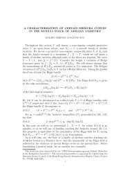
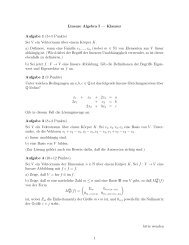
7. You should see a screen like that shown in Figure 1
Figure 1: Siena Data Entry Screen
8

8. If the initial screen appears correctly, then check your working directory or folder.
This is the directory that is opened immediately when clicking the Add button.
Various problems can be avoided by making sure that the working directory is the
directory that also contains the data files and the saved session file (see below)!
You need to have permission to write files in the working directory, and the data
files you want to use need to be in the same directory. To change the directory:
(a) Right click on the shortcut, and select Properties. (if somehow you don’t have
permission to do this, try copying the shortcut and pasting to create another
with fewer restrictions. (This may not work in Windows 7: you may need to
copy it from the visible desktop and then paste it in Windows Explorer in your
personal Desktop area.)) In the Start in: field type the name of the directory in
which you wish to work, i.e., a directory in which you can both read and write
files. Then click OK.
(b) To run the examples, put the session file and the data files in the chosen directory
before starting RSiena.
(c) To use your own data, put that data in the chosen directory before starting
RSiena.
2.2.1 Using the graphical user interface from Mac or Linux
1. Install R (most recent version) as appropriate for your computer.
2. Within R, type
install.packages(”RSiena”)
To use the latest beta version, use
install.packages(”RSiena”, repos=”http://R-Forge.R-project.org”)
3. Navigate to the directory RSiena package, (which you can find from within R by
running system.file(package=”RSiena”)) and find a file called sienascript. Run this
to produce the Siena GUI screen.(You will probably have to change the permissions
first (e.g.
chmod u+x sienascript)).
4. If you want to use the GUI, you need tcl/tk installed. This is an (optional) part of
the R installation on Mac. On Linux, you may need to install Tcl/tk and the extra
Tcl/tk package tktable. On Ubuntu Linux, the following commands will do what is
necessary (perhaps version numbers must be adapted): 3
sudo apt-get install tk8.5
sudo apt-get install libtktable2.9
3 Thanks to Michael Schweinberger and Krists Boitmanis for supplying these commands.
9

2.2.2 Running the graphical user interface: more details
Originally RSiena provided access to the GUI interface direct from Windows. This is not
now possible. This section details some helpful notes about starting RSiena within R 4 .
This is done by starting up R and working with the following commands. Note that R is
case-sensitive, so you must use upper and lower case letters as indicated.
First, set the ‘working directory’ of the R session to the same directory that holds the
data files; for example,
setwd(’C:/SienaTest’)
(Note the forward slash 5 , and the quotes are necessary 6 .) Windows users can use the
Change dir... option on the File menu.
You can use the following commands to make sure the working directory is what you
intend and see which files are included in it:
getwd()
list.files()
Assuming you see the data files, then you can proceed to load the RSiena package, with
the library function:
library(RSiena)
The other packages will be loaded as required, but if you wish to examine them or use
other facilities from them you can load them using:
library(network)
The following command will give a review of the functions that RSiena offers:
library(help=RSiena)
After that, you can use the RSiena GUI. It will ‘launch’ out of the R session.
siena01Gui()
You can monitor the R window for error messages – sometimes they are informative.
When you are done, quit R in the polite way:
q()
(Windows users may quit from the File menu or by closing the window.)
2.2.3 Entering Data.
There are two ways to enter the data.
1. Enter each of your data files using Add.
Fill in the various columns as described in Section 2.2.5.
2. If you have earlier saved the specification of data files, e.g., using Save to file, then
you can use Load new session from File.
This requires a file in the format described at the end of Section 2.2.5; such a file
can be created and read in an editor or spreadsheet program, and it is created in
.csv (comma separated) format by the siena01Gui() when you request Save to file.
4 We are grateful to Paul Johnson for supplying these ideas.
5 You can use backward ones but they must be doubled: setwd(’C:\\SienaTest’).
6 Single or double, as long as they match.
10

3. If you wish to remove files, use the Remove option rather than blanking out the
entries.
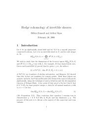
Once you have done this, check that the Format, Period, Type, etc., are correct, and enter
any values which indicate missingness in the Missing Values column. A (minimal) complete
screen is shown in Figure 2. The details of this screen are explained in Section 2.2.5.
Figure 2: Example of a Completed Data Entry Screen
2.2.4 Running the Estimation Program
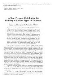
1. Click Apply: you will be prompted to save your work. Then you should see the
Model Options screen shown in Figure 3. If this does not happen, then one possible
Figure 3: Model options screen
source of error is that the program cannot find your files; e.g., the files are not in
the working directory (see above) but in a different directory.
If errors occur at this moment and the options screen does not appear, then you can
obtain diagnostic error messages working not through the siena01Gui, but directly
11

within R as described in Section 2.3.1. This will hopefully help you solving this
problem; later on you can then work through the siena01Gui again.
2. Select the options you require.
3. Use Edit Effects to choose the effects you wish to include. Note you can edit the effects
for just one dependent variable at a time if you wish by selecting one dependent
variable in ‘Effects dependent variable’.
4. Click Estimate.
5. You should see the SIENA screen of the estimation program.
6. When the program has finished, you should see the results. If not, click Display
Results to see the results. The output file which you will see is stored, with extension
.out in the directory in which you start siena.exe.
7. You may restart your estimation session at a later date using the Continue session
from file on the Data Entry Screen.
The restart needs a saved version of the data, effects and model as R objects. This
will be created automatically when you first enter the Model Options Screen, using
the default effects and model. You may save the current version at any time using
the Save to file button, and will be prompted to do so when you leave this screen.
2.2.5 Details of The Data Entry Screen
Group May be left blank unless you wish to use the multi-group option described in Section
11.1. Should not contain embedded blanks.
Name Network files or dyadic covariates should use the same name for each file of the
set. Other files should have unique names, a list of space separated ones for constant
covariates.
File Name Usually entered by using a file selection box, after clicking Add.
Format Only relevant for networks or dyadic covariates. Can be a matrix; a single Pajek
network (.net) (not for two-mode networks); or a Siena network file (an edgelist,
containing three or four columns: (from, to, value, wave (optional)), not yet tested
for dyadic covariates!). By specifying the waves in the fourth column in the Siena
format, one file can be used to contain data for all the waves.
Period(s) Only relevant for networks and dyadic covariates. All other files cover all the relevant
periods. Indicates the order of the network and dyadic covariate files. Should
range from 1 to M within each group, where M is the number of time points (waves).
Use multiple numbers separated by spaces for multi-wave Siena network files.
ActorSet If you have more than one set of nodes, use this column to indicate which is
relevant to each file. Should not contain embedded blanks.
12

Type Indicate here what type of data the file contains. Options are:
network (i.e., a one-mode network, which is the usual type)
bipartite (i.e., a two-mode network, which is a network with two node sets, and all
ties are between the first and the second node set)
behavior
constant covariate
changing covariate
constant dyadic covariate
changing dyadic covariate
exogenous event (for changing composition of the actor set)
Selected Yes or No. Files with Yes or blank will be included in the model. Use this field
to remove any networks or behavior variables that are not required in the model.
Missing Values Enter any values which indicate missingness, with spaces between different
entries.
Nonzero Codes Enter any values which indicate ties, with spaces between different entries.
NbrOfActors For Siena network files, enter the number of actors. For Siena net bipartite
files, enter the two dimensions (number of rows, number of columns) of the network,
separated by a blank space.
The details of the screen can be saved to a session file, from which they can be reloaded.
But you can create a session file directly: it should have columns with exactly the same
names and in exactly the same order as those of the Data Entry screen, and be of any of
the following types:
Extension Type
.csv Comma separated
.dat or .prn Space delimited
.txt Tab delimited
The root name of this input file will also be the root name of the output file.
2.2.6 Continuing the estimation
1. Below you will see some points about how to evaluate the reliability of the results.
If the convergence of the algorithm is not quite satisfactory but not extremely poor,
then you can continue just by Applying the estimation algorithm again.
2. If the parameter estimates obtained are very poor (not in a reasonable range), then
it usually is best to start again, with a simpler model, and from a standardized
starting value. The latter option must be selected in the Model Options screen.
13

2.3 Using SIENA within R
There are two alternatives, depending on your familiarity with R, treated in Sections 2.3.1
and 2.3.2. Section 2.3.3 explains how to make the step from the use of the GUI to the use
of R commands in the regular R way.
Section 2.4 presents an example of an R script for getting started with RSiena.
2.3.1 For those who are slightly familiar with R
1. Install R.
2. Install (within R) the package RSiena, and possibly network (required to read Pajek
files).
3. Set the working directory of R appropriately (setwd() within Ror via a desktop
shortcut).
4. You can get help by the command
help(RSiena)
This will open a browser window with help information; by clicking on the ‘Index’
link in the bottom line of this window, you get a window with all RSiena commands.
The command
RShowDoc("RSiena_Manual", package="RSiena")
opens the official RSiena manual.
5. Create a session file using siena01Gui() within R, or using an external program.
6. Then, within R,
(a) Use sienaDataCreateFromSession() to create your data objects.
(b) Use getEffects() to create an effects object.
(c) Use fix() to edit the effects object and select the required effects, by altering
the Include column to TRUE.
(d) Use sienaModelCreate() to create a model object.
(e) Use siena07() to run the estimation procedure.
Basic output will be written to a file. Further output can be obtained by using the
verbose=TRUE option of siena07.
14

2.3.2 For those fully conversant with R
1. Add the package RSiena
2. Get your network data (including dyadic covariates) into matrices, or sparse matrices
of type dgTMatrix. spMatrix() (in package Matrix) is useful to create the latter.
3. Covariate data should be in vectors or matrices.
4. All missing data should be set to NA.
5. Create SIENA objects for each network, behavior variable and covariate, using the
functions sienaNet() (for both networks and behavior variables), coCovar() etc.
6. Create a SIENA data object using SienaDataCreate().
7. Use getEffects() to create an effects object.
8. Use functions such as includeEffects(), setEffect(), and includeInteraction() to further
specify the model.
9. Use sienaModelCreate() to create a model object.
10. Use siena07() to run the estimation procedure.
11. Note that it is possible to use multiple processes in siena07. For details see section 2.6.
12. Also note the availability of the parameter prevAns to reuse estimates and derivatives
from a previous run with similar effects.
Basic output will be written to a file. Further output can be obtained by using the
verbose=TRUE option of siena07. The scripts on the scripts page of the RSiena website
give many examples of how to use RSiena.
2.3.3 The transition from using the graphical user interface to commands
At some moment, for users who started learning the use of RSiena through the GUI, it
can be desirable to make the transition to using commands in the regular R way. This
will make available more options and integration with other R features. The transition
can easily be made as follows.
After having made at least one estimation run in the GUI (which could be with the
default model specification, without having made any further additions to the model; but
it could also be with a more complicated model), click the button Save to file. You will be
prompted for a file name with extension .RData. Make sure that you do give a non-empty
name before the dot in .RData; for the moment, let us choose the name trans.RData.
Then later in an R session you can load the trans.RData. This can be done in Windows
by selecting File – Load Workspace from the drop down menu, and entering this file name.
It can also be done by entering the command
15

load("trans.RData")
This will make available three objects, for data, model, and effects. What is currently in
your workspace is shown by the command
ls()
This will probably show that the loaded objects have the names mydata, mymodel, and
myeff. These are the type of objects created by the functions sienaDataCreate, sienaModelCreate,
and getEffects, and discussed in the SIENA script in Section 2.4.
Now attach the package RSiena and subsequently ask for the descriptions of these three
objects:
library(RSiena)
mydata
mymodel
myeff
This will give short descriptions and thereby a confirmation of what has been imported
from the GUI session to the regular R session. From here on you can continue and work
with R commands, as in the script, to further specify the model by working on the effects
object, and then estimate the parameters by the siena07 function.
The precise point to continue from here, using the scripts in the next section and
also on the RSiena website, is to use script Rscript02SienaVariableFormat.R, starting with
section D (Defining Effects), part 3 (Adding/removing effects using includeEffects). After
this, you are advised to continue with script Rscript03SienaRunModel.R.
2.4 An example R script for getting started
The best way to get acquainted with RSiena is perhaps going through some existing
scripts. The script below is useful for this purpose. At the ‘RSiena scripts’ page http:
//www.stats.ox.ac.uk/~snijders/siena/siena_scripts.htm of the RSiena website it
is available divided into smaller pieces. The script is written so as to be useful for novice as
well as experienced R users. The ‘RSiena scripts’ page of the RSiena website also contains
some other scripts that may be useful. The appendix of this manual contains a list of
RSiena functions which may be consulted in addition to this script.
16

###################################################################################
###
### ---- Rscript01DataFormat.R: a script for the introduction to RSiena -------------
###
### version: January 17, 2012
###################################################################################
#
# Rscript01DataFormat.R is followed by
# RScriptSNADescriptives.R, code for descriptive analysis of the data, and
# Rscript02SienaVariableFormat.R, which formats data and specifies the model, and
# Rscript03SienaRunModel.R, which runs the model and estimates parameters
# Rscript04SienaBehaviour.R, which illustrates an example of analysing the
# coevolution of networks and behaviour
#
# The entire model fitting is summarised at the end of RscriptSienaRunModel.R
# (without comments)
#
# This is an R script for getting started with RSiena, written by
# Robin Gauthier, Tom Snijders, Ruth Ripley, Johan Koskinen, and
# Paulina Preciado, with some examples borrowed from Christian Steglich.
# Lines starting with # are not processed by R but treated as comments.
# The script has a lot of explanation of R possibilities that will be
# familiar for readers well acquainted with R, and can be skipped by them.
#
# There are various really easy online introductions to R. See, for example
#
# http://www.statmethods.net/
# http://www.burns-stat.com/pages/Tutor/hints_R_begin.html
# http://data.princeton.edu/R/gettingStarted.html
# http://www.ats.ucla.edu/stat/R/sk/
#
# You can go to any of these sites to learn the basics of R
# or refresh your knowledge.
# There is a lot of documentation available at
# http://cran.xl-mirror.nl/other-docs.html
# including some short introductions, handy reference cards,
# and introductions in many languages besides English.
#
#
# Some general points to note:
#
# R is case-sensitive. Be aware of capitalization!
#
# The left-arrow "

# That is why everything up to now in this file is on lines starting with #.
#
# This session will be using s50 data which are supposed to be
# present in the working directory.
# You can get them from
# http://www.stats.ox.ac.uk/~snijders/siena/siena_datasets.htm
#
# Any command in R is a function, and ends by parentheses
# that enclose the arguments of the function,
# or enclose nothing if no argument is needed, such as for the function q()
# In general the command syntax for calling R’s functions is function(x) where
# function is a saved function and x the name of the object to be operated on.
#
#################### - CALLING THE DATA AND PRELIMINARY MANIPULATIONS - ###########
# The library command loads the packages needed during the session.
library(RSiena)
# Some additional packages are used by RSiena,
# the so-called required packages; these will be loaded automatically.
# You need to have INSTALLED all of them.
?install.packages
# Or click on the tab "Packages", "Install package(s)", then select a CRAN mirror
# (e.g. Bristol if you are in the UK) and finally select from the list
# the package you wish to install.
# Where are you?
getwd()
# By something like
# setwd(’C:/SienaTest’)
# you can set the directory but note the quotes and forward slash.
# It is also possible to set the directory using the menus if you have them.
# On a windows machine, you can predetermine the working directory
# in the of the shortcut to R;
# these are accessible by right-clicking the shortcut.
# If you want to set the working directory to for example
# "C:\Documents and Settings\johan\My Documents\RSiena_course"
# simply copy and paste from windows explorer or type
# setwd(’C:/Documents and Settings/johan/My Documents/RSiena_course’)
# or
# setwd(’C:\\Documents and Settings\\johan\\My Documents\\RSiena_course’)
#
# but note that "\" has to be changed; both ’/’ and ’\\’ work!!!
# What is there?
list.files()
18

# What is available in RSiena?
?RSiena
# (these are .htlm HELP PAGES)
# At the bottom of this page, when you click on "Index",
# a list of all the available functions is shouwn in your browser.
# The same list is shown in the gui (’graphical user interface’) by requesting
library(help=RSiena)
# Where is the manual?
RShowDoc("RSiena_Manual", package="RSiena")
# (Note, however, that it is possible that the Siena website
# at http://www.stats.ox.ac.uk/~snijders/siena/ contains a more recent version.)
# Each data is named (for example below we name it friend.data.w1)
# so that we can call it as an object within R.
# If you read an object straight into R, it will treat it as a
# dataset, or in R terminology a "data frame".
# Here this is not what we want, therefore on reading
# we will immediately convert it to a matrix.
# R will read in many data formats, the command to read them is read.table.
?read.table
# In the help file for read.table, look at the section "Value",
# which is there in every help page:
# it indicates the class of the object that is produced by the function.
# For read.table, the value is a data frame; below we see what this is.
#
# If we wished to read a .csv file we would have
# used the read.csv command.
# The pathnames must have forward slashes, or double backslashes.
# If single backslashes are used, one of the error messages will be:
# 1: ’\R’ is an unrecognized escape in a character string
#-----------------------------------------------------------------------------
# Quick start(Data assignment).
# Please make sure the s50 data set is in your working directory.
# The data set is on the Siena website ("Data sets" tab) and must be
# unzipped in your working directory.
friend.data.w1

################# - DIFFERENT DATA FORMATS - #######################################
###
### The assignments here involve reading in data to a "data frame"
### data class(data)
### [1] "data.frame"
### If your data is not a ".dat" file, alternative import methods are
### ----- ".csv" ------------------------------------------------------------------
### data

attributes(data)
### ---- Matrix -------------------------------------------------------------------
### A "matrix" is a numeric object ordered like a matrix with dimensions
### ( dim() ) given by the number of rows and columns, e.g.
dim( friend.data.w1 )
### If you wish to play around with a copy of the matrix, e.g. having the name "data",
### you can make the copy by the command
data

### these reordered rows then are put into the object ArcList,
### this overwriting the earlier contents of this object.
### This way is tedious because it is repeated all the time that the names
### sid, recid, wid refer to the ArcList object.
### The less tedious way uses the function "with".
### The with(a, b) function tells R that b must be calculated,
### while the otherwise unknown names refer to data set a:
ArcList

### plot( test.net.1,main = test.net.1$gal$title )
### test.net.2

# This creates a logical vector which is TRUE for the cases where the condition
# is satisfied. To view or check, display the vectors:
drink[ , 1 ]
use
# and the number of selected cases is displayed by
# or
sum( use )
table( use )
# To have this arrayed more neatly side by side, you can create and display
# a matrix with the desired information,
aa

##################################################################################
###
### ---- RscriptSNADescriptives.R: a script for the introduction to RSiena -------
###
### version: January 17, 2012
##################################################################################
#
# Rscript01DataFormat.R is followed by
# RScriptSNADescriptives.R, code for descriptive analysis of the data, and
# Rscript02SienaVariableFormat.R, which formats data and specifies the model, and
# Rscript03SienaRunModel.R, which runs the model and estimates parameters
# Rscript04SienaBehaviour.R, which illustrates an example of analysing the
# coevolution of networks and behaviour
#
# The entire model fitting is summarised at the end of Rscript03SienaRunModel.R
# (without comments)
#
# This is an R script for getting started with RSiena, written by
# Robin Gauthier, Tom Snijders, Ruth Ripley, Johan Koskinen, and
# Paulina Preciado, with some examples borrowed from Christian Steglich.
# Lines starting with # are not processed by R but treated as comments.
# The script has a lot of explanation of R possibilities that will be
# familiar for readers well acquainted with R, and can be skipped by them.
# A visual inspection of the adjacency matrices can sometimes be useful.
# This will, for example, help in highlighting outliers with respect to
# outdegrees or indegrees, if there are any of such outliers.
# This requires package "sna":
library( network )
library( sna )
net1

# color the nodes by drink
plot( net1, vertex.col = "drink", xlab = ’friendship t1’ )
# Now let’s color the nodes by drink and scale the vertex by degree of nodes!
#
# First calculate degree:
deg

# ---- Basic network statistics ------------------------------------------------
# The package "sna" can be used for a variety of descriptions and analyses.
# The following are examples.
# some important graph level statistics
gden( net1 ) # density
grecip( net1 ) # proportion of dyads that are symmetric
grecip( net1, measure = "dyadic.nonnull" ) # reciprocity, ignoring the null dyads
gtrans( net1 ) # transitivity
# dyad and triad census
dyad.census( net1 )
triad.census( net1 )
# out degree distribution (of course for a symmetric network outdegree=indegree)
outdegree

# coevolution of networks and behaviour
# Written with contributions by Robin Gauthier, Tom Snijders, Ruth Ripley,
# Johan Koskinen, and Paulina Preciado.
#
# This script, Rscript02SienaVariableFormat.R, sets up the variables for analysis.
# The manipulations in this script requires that you have gone through the
# first part, "CALLING THE DATA AND PRELIMINARY MANIPULATIONS",
# of the script "Rscript01DataFormat.R" beforehand;
# or that you have defined the data and the model by means of the
# siena01Gui() function and have saved and loaded the results,
# as described in Section 2.3.3 of the Siena manual.
#### FORMATING DATA ACCORDING TO THEIR ROLES AS VARIABLES IN A SIENA MODEL #####
# A number of objects need to be created in R, as preparations to letting
# siena07 execute the estimation. This will be indicated by
# A: dependent variables;
# B: explanatory variables;
# C: combination of dependent and explanatory variables;
# D: model specification.
# ---- A. ----------------------------------------------------------------------
# First we have to create objects for the dependent variables.
# sienaNet creates a Siena network object from a matrix or array or list of
# sparse matrix of triples.
# This object will have the role of a dependent variable in the analysis.
# The name of this network object (here: friendship) will be used
# in the output file.
friendship

# friendship
# but this gives a lot of output which you may not want,
# hence the # sign in front.
# The function sienaNet can also be used to create a behavior variable object
# with the extra argument type = "behavior".
# (Non-mentioned attributes get the default value, and in this case
# oneMode is the default; see below.)
# The ’drink’ data (created in RscriptDataFormat.R ) is made available as a
# dependent behavior variable by the function
drinkingbeh

# ?varCovar
# ?coDyadCovar
# ?varDyadCovar
# ?sienaCompositionChange
# The variables available for this data set all are changing actor covariates.
# For illustrative purposes, we use smoking as observed at the first wave
# as a constant covariate:
smoke1

# mydata

# The rows of myeff correspond to the effects.
# By requesting
names( myeff )
# you see the type of information that is stored about the effects,
# i.e., the columns (variables) defined for the effects.
# If desired, more information about these variables can be obtained
# from the help files:
# ?getEffects
# Among these variables is the effectName.
# The set of available effects can be inspected by requesting their names:
myeff$effectName
# This gives a lot of names: all effects defined in Section 12 of the manual,
# depending on the variables specified in mydata.
# The "include" column defines whether effects are included in the model.
myeff$include
# Here the TRUE values correspond to the default model specification which,
# however, is not meant as a serious model, being too limited.
# There are 3 main ways to operate on myeff.
# 1. Changing myeff in spreadsheet form by the function fix();
# 2. Changing myeff directly by operating on its elements;
# 3. Using RSiena functions "includeEffects", "setEffects", etc.
# Which one to use is a matter of personal preference.
# The third way is most in line with the design philosophy of R,
# and allows you to save scripts that also can be used when
# there will be new versions of RSiena.
# Therefore, we suggest that you skip the explanations of options 1 and 2, and
# proceed directly to option 3, ’ Adding/removing effects using includeEffects’.
# For identifying your effects you need the "shortName"s,
# which can be read in the manual (section "Mathematical definition of effects"),
# or obtained from the "sink" command below.
# ---- 1. Adding/removing effects using fix() ----------------------------------
# fix calls a data editor internal to R, so we can manually edit the effects.
# This operates the same as in the Gui.
fix( myeff )
# How to use fix() is presented merely for getting to know what myeff is.
# In practical analysis it is more convenient
# to use routine "includeEffects" instead, as explained below.
# fix() may not be usable if you do not have tcl/tk available!
# Note that the top of the dataframe shows the names of the columns:
# name, effectName, etc.
# You can edit the "include" column by changing the TRUE and FALSE values
# as required; when the editor is closed, the new values are stored.
32

# ---- 2. Adding/removing effects by direct manipulation of myeff --------------
# Alternatively we can edit the dataframe directly by using R functions.
# You are advised to skip this part ("2.") at first reading,
# and read it only if you wish to get more understanding
# of the interal strtucture of the effects object.
# The commands below are used to set "include" to TRUE or FALSE,
# as an alternative to using the data editor.
# The "include" column with values TRUE or FALSE will always be
# ocated at the 9th column,
# but transitive triplets will not always be at the 13th row as this depends
# on the number of periods and variables; further, the list of available effects
# may change in future versions.
# Note: These row numbers may not be the current ones, as they depend on the
# list of effects implemented, which is changeable.
# Some examples are the following
# (preceded by # because not proposed to be applied).
#myeff[13,9]

# write.table(format(cbind( myeff$effectName,myeff$shortName)),"effectlist.txt")
# Now look in the file "effectlist.txt" (in the current directory)
# for the spelling of the various effects you might wish to use.
# The following commands can be used to select the
# five mentioned effects.
# Note that == is the logical "equals", & is the logical "and",
# and what is between the square brackets [...] makes a selection
# of the specified row and column of the "myeff" data frame.
myeff[myeff$effectName==’transitive triplets’ &
myeff$type==’eval’, ’include’]

myeff

# A convenient method to include an interaction is offered by the
# includeInteraction function.
# This can be used to interact two or three effects
# (if the interactions are allowed; see the manual for this).
# The interaction between smoke1 ego and reciprocity, for instance,
# can be defined by the command
myeff

#
# The introductory script is divided into the following script files:
# Rscript01DataFormat.R, followed by
# RScriptSNADescriptives.R, code for descriptive analysis of the data, and
# Rscript02SienaVariableFormat.R, which formats data and specifies the model, and
# Rscript03SienaRunModel.R, which runs the model and estimates parameters
# Rscript04SienaBehaviour.R, which illustrates an example of analysing the
# coevolution of networks and behaviour.
# Written with contributions by Robin Gauthier, Tom Snijders, Ruth Ripley,
# Johan Koskinen, and Paulina Preciado.
#
# This script, Rscript03SienaRunModel.R, runs the estimation in RSiena for the
# model set up and defined in the script Rscript02SienaVariableFormat.R.
#
# A quick version of the model fitting without comments is given at the end
# of this script
########################### ESTIMATION OF PARAMETERS ###########################
# Parameters of the model are estimated by the function siena07.
# This requires the data specification; the effects specification;
# and a number of parameters, or settings, for the estimation algorithm.
# The latter are contained in an object created by the function sienaModelCreate.
# You can look at the help provided by ?sienaModelCreate
# to find out about options that you may use here;
# for beginning users, only the two options mentioned below are relevant.
#
# Output will be written to a file with name projname.out, where projname is
# whatever name is given; the default (used if no name is given) is Siena.
# This file will be written to your current directory.
# New estimation runs will append to it.
# A new call to print01Report will overwrite it!
mymodel

# ans

################### LOOKING AT THE RESULTS ################################
# The file "s50_3.out" will contain the results of the estimation.
# It is contained in the current directory ("getwd()").
# This file can be read by any text editor.
# A summary of the results is obtained on the screen by
ans
# and a larger summary by
summary(ans)
# Depending on the random seed and the model specification,
# the results could be something like the following.
# Estimates, standard errors and t-statistics for convergence
#
# Estimate Standard t statistic
# Error
#
# Rate parameters:
# 0.1 Rate parameter period 1 6.5644 ( 1.1020 )
# 0.2 Rate parameter period 2 5.1981 ( 0.8611 )
#
# Other parameters:
# 1. eval outdegree (density) -2.7027 ( 0.1253 ) -0.0025
# 2. eval reciprocity 2.3894 ( 0.2157 ) -0.0335
# 3. eval transitive triplets 0.6111 ( 0.1392 ) -0.0247
# 4. eval 3-cycles -0.0069 ( 0.2731 ) 0.0126
# 5. eval smoke1 similarity 0.2595 ( 0.2107 ) 0.0144
# 6. eval alcohol alter -0.0195 ( 0.0699 ) -0.0155
# 7. eval alcohol ego 0.0374 ( 0.0801 ) -0.0681
# 8. eval alcohol ego x alcohol alter 0.1297 ( 0.0527 ) -0.0001
#
# The results can also be viewed externally in the output file s50_3.out
# It is advisable that you have a look at all three reports and
# understand how information is organized in each of them.
# To understand the table above, note that the "t statistic"
# is the t-statistic for convergence checking,
# not the t statistic for testing the significance of this effect!
# (See Section 6.2 of the manual.)
# In the external output file, these are called
# "t-ratios for deviations from targets".
# The rule of thumb is that all t-ratios for convergence
# should ideally be less than 0.1 in absolute value;
# this signifies good convergence of the algorithm.
# In the example here, this is the case.
# If this would not be the case, the best thing to do would be
# to continue the estimation, using the estimates produced here,
# and contained in ans, as the new initial values.
# This is explained below.
39

# With function siena07 we made ans as the object containing
# all the results of the estimation. For example,
ans$theta
# contains the vector of parameter estimates while
ans$covtheta
# contains the covariance matrix of the estimates.
# There are several "methods" available for viewing the object
# containing the results of the estimation.
# Above we already mentioned
# ans
# and
# summary( ans )
# The command
xtable( ans )
# will produce a table formatted for inclusion in a LaTeX document
# or formatted in html. Use e.g.
xtable( ans, type = ’html’ )
# to get html, and e.g.
xtable( ans, file = ’ff.tex’ )
# to write the results to a file.
# At http://cran.r-project.org/web/packages/xtable you can find
# a set of vignettes for the xtable package, the xtable gallery,
# which gives more options.
# A function siena.table is available that is specially designed
# for RSiena results.
############## MORE ON INITIALIZING PARAMETERS FOR ESTIMATION ########
# If the estimation algorithm has not produced good estimates
# (it ’has not converged well’),
# as will be indicated by some of the t-ratios for convergence
# being larger than 0.1 (this threshold is not to be taken too precisely, though),
# the best thing to do is continuing the estimation,
# using the estimates produced here,
# and contained in ans, as the new initial values.
# This is done by the option prevAns (’previous ans’) as in
ans

# This should be used only if the model specification in myeff
# has not changed, and if the provisional parameter estimates obtained
# in ans are reasonable; if they are not reasonable,
# omit the prevAns option, use
# mymodel$useStdInits

# myeff

myeff

# "friends" with respect to behaviour (like Moran’s I) are given by the function
# nacf() in the sna package
# Tell RSiena that the adjacency matrices are network data and in what order
# they should be treated
friendship

myCoEvolutionEff
# Define the model as data + effects:
myCoEvModel

(a) In Phase 1, the sensitivity of the statistics to the parameters is roughly determined.
(b) In Phase 2, provisional parameter values are updated:
this is done by simulating a network according to the provisional parameter
values, calculating the statistics and the deviations between these simulated
statistics and the target values, and making a little change (the ‘update’) in the
parameter values that hopefully goes into the right direction.
(Only a ‘hopefully’ good update is possible, because the simulated network is
only a random draw from the distribution of networks, and not the expected
value itself.)
(c) In Phase 3, the final result of Phase 2 is used, and it is checked if the average
statistics of many simulated networks are indeed close to the target values. This
is reflected in the so-called t statistics for deviations from targets.
2.6 Using multiple processes
1. If multiple processors are available, then using multiple processes can speed up the
estimation in siena07.
2. In Phases 1 and 3 the simulations are performed in parallel. In Phase 2, multiple
simulations are done with the same parameters, and the resulting statistics are averaged.
The gain parameter is increased and the number of iterations in phase 2
reduced to take advantage of the increased accuracy.
3. The parameters required to run all processes on one computer are fairly simple: in
your call to siena07, set nbrNodes to the number of processes and useCluster and
initC to TRUE. The Model Options screen also allows you to specify the number of
processes, and will automatically set the other required parameters for you.
4. To use more than one machine is more complicated, but it can be done by using, in
addition, the clusterString parameter. The computers need to be running incoming
ssh.
5. For machines with exactly the same layout of R directories on each, simply set
clusterString to a character vector of the names of the machines.
6. For other cases, e.g. using Macs alongside Linux, see the documentation for the
package parallel.
7. RSiena uses sockets for inter-process communication.
8. On Windows, sub processes are always started using R scripts. On Linux and Mac
there is an option available in R version 2.14.0 or later via the code interface to
siena07 to ask for the sub processes to be formed by forking. See the help page for
details.
46

9. Each process needs a copy of the data in memory. If there is insufficient memory
available there will be no speed gain as too much time will be spent paging.
10. In each iteration the main process waits until all the other processes have finished.
The overall speed is therefore that of the slowest process, and there should be enough
processors to allow them all to run at speed.
2.7 Steps for looking at results: Executing SIENA.
1. Look at the start of the output file for general data description (degrees, etc.), to
check your data input.
2. When parameters have been estimated, first look at the t ratios for deviations
from targets. These are good if they are all smaller than 0.1 in absolute value,
and reasonably good if they are all smaller than 0.2.
We say that the algorithm has converged if they are all smaller than 0.1 in absolute
value, and that it has nearly converged if they are all smaller than 0.2.
These bounds are indications only, and may be taken with a grain of salt.
3. In rare circumstances, when the data set leads to instability of the algorithm, the
following may be of use.
The Initial value of the gain parameter determines the step sizes in the parameter
updates in the iterative algorithm. This is the parameter called firstg in function
sienaModelCreate. A too low value implies that it takes very long to attain a reasonable
parameter estimate when starting from an initial parameter value that is
far from the ‘true’ parameter estimate. A too high value implies that the algorithm
will be unstable, and may be thrown off course into a region of unreasonable (e.g.,
hopelessly large) parameter values.
It usually is unnecessary to change this.
4. If all this is of no avail, then the conclusion may be that the model specification is
incorrect for the given data set.
5. Further help in interpreting output is in Section 6.4 of this manual.
2.8 Giving references
When using SIENA, it is appreciated that you refer to this manual and to one or more
relevant references of the methods implemented in the program. The reference to this
manual is the following.
Ripley, Ruth M., Snijders, Tom A.B., and Preciado, Paulina. 2011. Manual for SIENA
version 4.0 (version March 29, 2012). Oxford: University of Oxford, Department of Statistics;
Nuffield College. http://www.stats.ox.ac.uk/siena/
A basic reference for the network dynamics model is Snijders (2001) or Snijders (2005).
Basic references for the model of network-behavior co-evolution are Snijders et al. (2007)
47

and Steglich et al. (2010). A basic reference for the Bayesian estimation is Koskinen and
Snijders (2007) and for the maximum likelihood estimation Snijders et al. (2010b).
More specific references are Schweinberger (2011) for the score-type goodness of fit
tests and Schweinberger and Snijders (2007b) for the calculation of standard errors of
the Method of Moments estimators. For assessing and correcting time heterogeneity, and
associated model selection considerations, refer to Lospinoso et al. (2011).
A tutorial is Snijders et al. (2010a).
2.9 Getting help with problems
If you have a problem running RSiena, please read through the following hints to see if any
of them help. If not, please send an email to rsiena-help@lists.r-forge.r-project.org, or post
in the help forum for RSiena in R-forge. You need to be a registered member of R-forge
(and possibly of RSiena) to post to a forum, but anyone can send emails (at present!).
In your message, please tell us which operating system , which version of R, and which
version of RSiena you are using.
For queries about the modelling aspects of SIENA, or interpretation, please continue
to use the StOCNET / RSiena mailing list.
Check your version of RSiena Details of the latest version available can be found at
http://r-forge.r-project.org/R/?group_id=461. The version is identified by a
version number (e.g. 1.0.9) and an R-forge revision number. You can find both the
numbers of your current installed version by opening R , and typing
packageDescription("RSiena"). The version is near the top, the revision number
near the end. Both are also displayed at the start of SIENA output files (use
print01Report to get the relevant output file if you are not using the GUI.)
Check your version of R When there is a new version or revision of RSiena it will only
be available to you automatically if you are running the most recent major version
of R. (You can force an installation if necessary by downloading the tarball or binary
and installing from that, but it is better to update your R.)
Check both repositories We have two repositories in use for RSiena: CRAN and Rforge.
The latest version will always be available from R-forge. (Frequent updates
are discouraged on CRAN, so bug-fixes are likely to appear first on R-forge.)
Installation When using the repository at R-forge, install the package rather than updating
it. Then check the version and revision numbers.
48

Part II
Users’ manual
3 Parts of the program
The operation of the SIENA program is comprised of five main parts:
1. input of basic data description,
2. model specification,
3. estimation of parameter values using stochastic simulation,
4. testing parameters and assessing goodness of fit,
5. simulation of the model with given and fixed parameter values.
The normal operation is to start with data input, then specify a model and estimate
its parameters, assess goodness of fit and the significance of the parameters, and then
possibly continue with new model specifications followed by estimation or simulation.
The main output is written to a text file named pname.out, where pname is the name
specified in the call of sienaModelCreate().
49

4 Input data
SIENA is a program for the statistical analysis of repeated measures of social networks,
and requires network data collected at two or more time points. It is possible to include
changing actor variables (representing behavior, attitudes, outcomes, etc.) which also
develop in a dynamic process, together with the social networks. As repeated measures
data on social networks, at the very least, two or more repeated observations of a network
are required. The number of time points is denoted M.
In addition, various kinds of variables are allowed:
1. actor-bound or individual variables, also called actor attributes, which can be symbolized
as vi for each actor i; these can be constant over time or changing;
the changing individual variables can be dependent variables (changing dynamically
in mutual dependence with the changing network; then they are also called dependent
behavior variables) or independent variables (exogenously changing variables;
then they are also called individual covariates).
2. dyadic covariates, which can be symbolized as wij for each ordered pair of actors
(i, j); these likewise can be constant over time or changing.
Dependent variables (which can be networks or behavior variables) all must be available
for the same set of time points.
It is advisable to use names of variables consisting of at most 12 characters. This is
because they are used as parts of the names of effects which can be included in the model,
and the effect names should not be too long.
The data specification in RSiena consists of two steps. First, the role of each variable
to be used must be defined using the functions sienaNet, coCovar, varCovar, coDyadCovar,
varDyadCovar, or sienaCompositionChange. Second, the variables must be combined into
one RSiena data set by the function sienaDataCreate.
4.1 Digraph data
For data specification by the sienaNet function, the network must be specified as a matrix
or array or list of sparse matrix of triples. The help file for sienaNet shows by examples how
the specification can be given by sparse matrices. Here we only discuss the specification
by matrices.
For data specification by the graphical interface siena01Gui or by the function siena-
DataCreateFromSession, edge list formats are also allowed. This can be either the format
of the Pajek program, or a raw edge list, here called Siena format. For large number
of nodes (say, larger than 100), the edge list format is more efficient in use of computer
memory. The three possible formats for digraph input are as follows.
1. Adjacency matrices.
These can be used in sienaNet and in sienaDataCreateFromSession.
In the usual case of a one-mode network the adjacency matrix consists of n lines
50

each with n integer numbers, separated by blanks or tabs, each line ended by a hard
return. The diagonal values are meaningless but must be present. In the case of a
two-mode network (which is a network with two node sets, and all ties are between
the first and the second node set) the matrix does not have to be square, as usually
the number of nodes in the first set will not be equal to the number of nodes in the
second set; and if it would be square, the diagonal still would be meaningful.
Although this section talks only about digraphs (directed graphs), for one-mode
networks it is also possible that all observed adjacency matrices are symmetric.
This will be automatically detected by SIENA, and the program will then utilize
methods for non-directed networks.
The values of the ties must be 0, 1, or NA (not available = missing); or 10 or 11 for
structurally determined values (see below).
2. Pajek format.
These can be used in sienaDataCreateFromSession.
If the digraph data file has extension name .net, then the program assumes that the
data file has Pajek format. The file should relate to one observation only, and should
contain a list of vertices (using the keyword *Vertices, together with (currently) a
list of arcs, using the keyword *Arcs followed by data lines according to the Pajek
rules. These keywords must be in lines that contain no further characters. An
example of such input files is given in the s50 data set that is distributed in the
examples directory of the source code.
3. Siena format.
These can be used in sienaDataCreateFromSession.
An edge list is a matrix containing three or four columns: from, to, value, wave
(optional).
Like the Pajek format, this has the advantage that absent ties (tie variables with the
value 0) do not need to be mentioned in the data matrix. By specifying the waves
in the fourth column in the Siena format, one matrix can be used to contain data
for all the waves.
Missing values must be indicated in the way usual for R, by NA. For data specification by
the graphical interface siena01Gui or by the function sienaDataCreateFromSession, instead
of NA any numerical code can be used given that this is indicated to be a missing value
code.
If the data set is such that it is never observed that ties are terminated, then the
network dynamics is automatically specified internally in such a way that termination of
ties is impossible. (In other words, in the simulations of the actor-based model the actors
have only the option to create new ties or to retain the status quo, not to delete existing
ties.) Similarly if ties never are created (but only terminated), then this will be respected
in the simulations.
51

4.1.1 Transformation between matrix and edge list formats
The following R commands can be used for transforming an adjacency matrix to an edge
list, and back again. If a is an adjacency matrix, then the following commands can be
used to create the corresponding edge list, called edges here.
# create indicator matrix of non-zero entries of a
ones

should return the value 0.
Note that the basic edge list, edges, lacks information as to the size of the adjacency
matrix. tmp above is a sparse matrix which is in edge list format but includes information
on the size of the adjacency matrix, and can be used in a similar way to the original matrix
a while saving memory space.
4.1.2 Structurally determined values
It is allowed that some of the values in the digraph are structurally determined, i.e.,
deterministic rather than random. This is analogous to the phenomenon of ‘structural
zeros’ in contingency tables, but in SIENA not only structural zeros but also structural
ones are allowed. A structural zero means that it is certain that there is no tie from actor
i to actor j; a structural one means that it is certain that there is a tie. This can be, e.g.,
because the tie is impossible or formally imposed, respectively.
Structural zeros provide an easy way to deal with actors leaving or joining the network
between the start and the end of the observations: specify all their incoming and outgoing
tie variables, at the moment that they are not present, as structural zeros. Note that actors
having all values specified as structural zeros in this way take part of the simulations only
starting at the observation moment where they are not totally structurally zero; therefore,
this way of representing partially absent actors is not meaningful for actors who are present
only at the very last wave. Note that this always includes the case where there are two
waves only for actors who join the network after the first wave.
Another way (more complicated but more flexible, because it gives possibilities to
represent actors entering or leaving at specified moments between observations) is the
method of joiners and leavers, described in Section 4.8. For actors present only at the last
wave, the method of joiners and leavers is preferable.
Structurally determined values are defined by reserved codes in the input data: the
value 10 indicates a structural zero, the value 11 indicates a structural one. Structurally
determined values can be different for the different time points. (The diagonal of the data
matrix for a one-mode network always is composed of structural zeros, but this does not
have to be indicated in the data matrix by special codes.) The correct definition of the
structurally determined values can be checked from the brief report of this in the output
file.
If there are a lot of structurally determined values then unconditional estimation (see
Section 6.6.1) is preferable.
Structural zeros offer the possibility of analyzing several networks simultaneously under
the assumption that the parameters are identical. Another option to do this is given in
Section 11. E.g., if there are three networks with 12, 20 and 15 actors, respectively, then
these can be integrated into one network of 12 + 20 + 15 = 47 actors, by specifying that
ties between actors in different networks are structurally impossible. This means that the
three adjacency matrices are combined in one 47 × 47 data matrix, with values 10 for all
entries that refer to the tie from an actor in one network to an actor in a different network.
In other words, the adjacency matrices will be composed of three diagonal blocks, and the
off-diagonal blocks will have all entries equal to 10. In this example, the number of actors
53

per network (12 to 20) is rather small to obtain good parameter estimates, but if the
additional assumption of identical parameter values for the three networks is reasonable,
then the combined analysis may give good estimates.
In such a case where K networks (in the preceding paragraph, the example had K = 3)
are combined artificially into one bigger network, it will often be helpful to define K − 1
dummy variables at the actor level to distinguish between the K components. These
dummy variables can be given effects in the rate function and in the evaluation function
(for “ego”), which then will represent that the rate of change and the out-degree effect are
different between the components, while all other parameters are the same.
It will be automatically discovered by SIENA when functions depend only on these
components defined by structural zeros, between which tie values are not allowed. For
such variables, only the ego effects are defined and not the other effects defined for the
regular actor covariates and described in Section 5.4. This is because the other effects
then are meaningless. If at least one case is missing (i.e., has the missing value data code
for this covariate), then the other covariate effects are made available.
When SIENA simulates networks including some structurally determined values, if
these values are constant across all observations then the simulated tie values are likewise
constant. If the structural fixation varies over time, the situation is more complicated.
Consider the case of two consecutive observations m and m + 1, and let Xsim be the simu-
ij
lated value at the end of the period from tm to tm+1. If the tie variable Xij is structurally
fixed at time tm at a value xij(tm), then X sim
ij also is equal to xij(tm), independently of
whether this tie variable is structurally fixed at time tm+1 at the same or a different value
or not at all. This is the direct consequence of the structural fixation. On the other hand,
the following rule is also used. If Xij is not structurally fixed at time tm but it is structurally
fixed at time tm+1 at some value xij(tm+1), then in the course of the simulation
process from tm to tm+1 this tie variable can be changed as part of the process in the
usual way, but after the simulation is over and before the statistics are calculated it will
be fixed to the value xij(tm+1).
The target values for the algorithm of the Method of Moments estimation procedure
are calculated for all observed digraphs x(tm+1). However, for tie variables Xij that are
structurally fixed at time tm, the observed value xij(tm+1) is replaced by the structurally
fixed value xij(tm). This gives the best possible correspondence between target values and
simulated values in the case of changing structural fixation.
4.2 Dependent behavioral variables
Dependent actor-level variables, also called dependent behavior variables, are changing
variables at the actor level, analysed according to the “networks and behavior” actororiented
model of Snijders et al. (2007); Steglich et al. (2010). This means they change
dynamically in mutual dependence with the changing network. These variables also are
defined using the sienaNet function, now requiring the type = behavior parameter.
54

4.3 Dyadic covariates
Like the digraph data, also each measurement of a dyadic covariate must be contained
in a separate matrix. For one-mode data this is a square data matrix, and the diagonal
values are meaningless.
A distinction is made between constant and changing dyadic covariates, where change
refers to changes over time. Each constant covariate has one value for each pair of actors,
which is valid for all observation moments, and has the role of an independent variable.
Changing covariates, on the other hand, have one such value for each period between
measurement points. If there are M waves (i.e., observation moments) of network data,
this covers M−1 periods, and accordingly, for specifying a single changing dyadic covariate,
M − 1 covariate matrices are needed.
Constant dyadic covariates are specified using function coDyadCovar, and changing
dyadic covariates by varDyadCovar.
The mean is always subtracted from the covariates. See Section 4.9 on centering.
4.4 Individual covariates
Individual (i.e., actor-bound, or monadic) variables are defined by the functions coCovar
in the case they are constant over time, and varCovar if they are changing over time.
Each constant actor covariate has one value per actor valid for all observation moments,
and has the role of an independent variable.
Changing variables can change between observation moments; then they are called
‘changing individual covariates’, and have the role of independent variables.
Changing individual covariates are assumed to have constant values from one observation
moment to the next. If observation moments for the network are t1, t2, ..., tM, then
the changing covariates should refer to the M − 1 moments t1 through tM−1 , and the
m-th value of the changing covariates is assumed to be valid for the period from moment
tm to moment tm+1 . The value at tM, the last moment, does not play a role. Changing
covariates, as independent variables, are meaningful only if there are 3 or more observation
moments, because for 2 observation moments the distinction between constant and
changing covariates is not meaningful.
Each changing individual covariate must be specified in a separate call fo varCovar,
using for input an n × M − 1 matrix where the columns correspond to the M − 1 periods
between observations.
The mean is always subtracted from the covariates. See Section 4.9 on centering.
When an actor covariate is constant within waves, i.e., within each wave it has the same
value for all actors; or, more generally, when within each wave it has the same value for all
actors within components separated by structural zeros (which means that ties between
such components are not allowed), then only the ego effect of the actor covariate is made
available. This is because the other effects then are meaningless. This may cause problems
for combining several data sets in a multi-group project (see Section 11). If at least one
case is missing (i.e., has the missing value data code), then the other covariate effects are
made available. When analysing multiple data sets in parallel, for which the same set of
55

effects is desired to be included, it is therefore advisable to give data sets in which a given
covariate has the same value for all actors one missing value in this covariate; purely to
make the total list of effects independent of the observed data.
4.5 Interactions and dyadic transformations of covariates
For actor covariates (also called monadic covariates), two kinds of transformations to
dyadic covariates are made internally in SIENA. Denote the actor covariate by vi, and
the two actors in the dyad by i and j. Suppose that the range of vi (i.e., the difference
between the highest and the lowest values) is given by rV . The two transformations are
the following:
1. dyadic similarity, defined by 1 −
|vi − vj|/rV , and centered so the the mean of this
similarity variable becomes 0;
note that before centering, the similarity variable is 1 if the two actors have the
same value, and 0 if one has the highest and the other the lowest possible value; the
mean of the similarity variable is calculated by function sienaDataCreate and stored
as the simMean attribute of mydata$cCovars$myvar, where mydata is the name of
the object created by sienaDataCreate, and myvar is the name of the variable used
as the argument for sienaDataCreate, while the name cCovars applies for constant
monadic covariates, and is to be replaced by vCovars for changing (varying) monadic
covariates;
2. same V , defined by 1 if vi = vj, and 0 otherwise (not centered) (V is the name of
the variable). This can also be referred to as dyadic identity with respect to V .
Dyadic similarity is relevant for variables that can be treated as interval-level variables;
dyadic identity is relevant for categorical variables.
In addition, SIENA offers the possibility of user-defined two- and three-variable interactions
between covariates; see Section 5.8.
4.6 Dependent action variables
SIENA also allows dependent action variables, also called dependent behavior variables.
This can be used in studies of the co-evolution of networks and behavior, as described
in Snijders et al. (2007) and Steglich et al. (2010). These action variables represent the
actors’ behavior, attitudes, beliefs, etc. The difference between dependent action variables
and changing actor covariates is that the latter change exogenously, i.e., according
to mechanisms not included in the model, while the dependent action variables change
endogenously, i.e., depending on their own values and on the changing network. In the
current implementation only one dependent network variable is allowed, but the number
of dependent action variable can be larger than one. Unlike the changing individual covariates,
the values of dependent action variables are not assumed to be constant between
observations.
56

Dependent action variables must have nonnegative integer values; e.g., 0 and 1, or a
range of integers like 0,1,2 or 1,2,3,4,5. Each dependent action variable must be given in
one matrix, containing k = M columns, corresponding to the M observation moments.
If any values are not integers, a warning will be printed on the initial report and the
values will be truncated towards zero.
4.7 Missing data
SIENA allows that there are some missing data on network variables, on covariates, and
on dependent action variables. Missing data in changing dyadic covariates are not yet
implemented. Missing data must be indicated by missing data codes, not by blanks in the
data set.
Missingness of data is treated as non-informative. One should be aware that having
many missing data can seriously impair the analyses: technically, because estimation will
be less stable; substantively, because the assumption of non-informative missingness often
is not quite justified. Up to 10% missing data will usually not give many difficulties or
distortions, provided missingness is indeed non-informative (Huisman and Steglich, 2008).
When one has more than 20% missing data on any variable, however, one may expect
problems in getting good estimates.
In the current implementation of SIENA, missing data are treated in a simple way,
trying to minimize their influence on the estimation results.
The basic idea is the following.
NOTE: This may not be a correct representation. To be modified.
A brief sketch of the procedure is that missing values are imputed to allow meaningful
simulations; for the calculation of the target statistics in the Method of Moments, tie
variables and actor variables with missings are not used. More in detail, the procedure is
as follows.
The simulations are carried out over all variables, as if they were complete. To enable
this, missing data are imputed. In the initial observation, missing entries in the adjacency
matrix are set to 0, i.e., it is assumed that there is no tie; this is done because normally data
are sparse, so ‘no tie’ is the modal value of the tie variable. In the further observations,
for any variable, if there is an earlier observed value of this variable then the last observed
value is used to impute the current value (the ‘last observation carry forward’ option, cf.
Lepkowski (1989)); if there is no earlier observed value, the value 0 is imputed. For the
dependent behavior variables the same principle is used: if there is a previous observation
of the same variable then this value is imputed, if there is none then the observationwise
mode of the variable is imputed. Missing covariate data are replaced by the variable’s
average score at this observation moment. In the course of the simulations, however, the
adjusted values of the dependent action variables and of the network variables are allowed
to change.
In order to ensure a minimal impact of missing data treatment on the results of parameter
estimation (method of moments estimation) and/or simulation runs, the calculation
of the target statistics used for these procedures uses only non-missing data. When for
57

an actor in a given period, any variable is missing that is required for calculating a contribution
to such a statistic, this actor in this period does not contribute to the statistic
in question. For network and dependent action variables, the tie variable or the actor
variable, respectively, must provide valid data both at the beginning and at the end of a
period for being counted in the respective target statistics.
4.8 Composition change
SIENA can also be used to analyze networks of which the composition changes over time,
because actors join or leave the network between the observations. This can be done in two
ways: using the method of Huisman and Snijders (2003), or using structural zeros. (For the
maximum likelihood estimation option, the Huisman-Snijders method is not implemented,
and only the structural zeros method can be used.) Structural zeros can specified for all
elements of the tie variables toward and from actors who are absent at a given observation
moment. How to do this is described in subsection 4.1.2. This is straightforward and
not further explained here. This subsection explains the method of Huisman and Snijders
(2003), also called the method of joiners and leavers, which uses the information about
composition change in a somewhat more efficient way.
Network composition change, due to actors joining or leaving the network, is handled
separately from the treatment of missing data. The digraph data matrices must contain
all actors who are part of the network at any observation time. If adjacency matrices are
used as data input, they must therefore all have the same number of n lines, each actor
having a separate (and fixed) line in these matrices, even for observation times where the
actor is not a part of the network (e.g., when the actor did not yet join or the actor already
left the network).
The times of composition change can be given either in a data file or in a list available
in the R session. For networks with constant composition (no entering or leaving actors),
this file or list is omitted and the current subsection can be disregarded.
At these times, where the actor is not in the network, the entries of the adjacency
matrix can be specified in two ways. First as missing values using missing value code(s).
In the estimation procedure, these missing values of the joiners before they joined the
network are regarded as 0 entries, and the missing entries of the leavers after they left the
network are fixed at the last observed values. This is different from the regular missing
data treatment. Note that in the initial data description the missing values of the joiners
and leavers are treated as regular missing observations. This will increase the fractions of
missing data and influence the initial values of the density parameter.
A second way is by giving the entries a regular observed code, representing the absence
or presence of a tie (as if the actor was a part of the network). In this case, additional
information on relations between joiners and other actors in the network before joining,
or leavers and other actors after leaving can be used if available. Note that this second
option of specifying entries always supersedes the first specification: if a valid code number
is specified this will always be used.
The functions used to specify the times actors join or leave the network (i.e., the times
of composition change) are sienaCompositionChangeFromFile in case a file is used, and
58

sienaCompositionChange in case a list is used. How to use a separate input file, called the
exogenous events file, is described in Section 2.1.
In the second case, a list must be given of length n, where n is the number of actors in
the node set. The i’th element of this list must be a vector of numbers (characters are also
allowed), composed of an even number of elements, indicating the intervals during which
actor i was present. For example, 1 4 indicates that the actor was present from wave 1
to wave 4 (end points included) and 1 3.2 5.01 7 indicates that the actor was present
from wave 1 to 20% of the time between waves 3 and 4, and then again from just after
wave 5 to wave 7.
As an example, suppose we have 50 actors and 6 waves; almost all actors were present
all the time, but actor 11 was present from wave 3 onward, actor 20 was present until
wave 4, and actor 33 was present from mid-way between waves 1 and 2 until wave 3, and
then again from just after wave 4 to wave 6. Then the list can be created by the following
commands.
comp

a different moment, but the effect is exactly the same.) Unlike the ‘covariate similarity’
effect, the ‘same covariate’ effect is not centered but keeps its 0-1 values.
For dependent behavioral variables, the effects are defined in Section 12.2 as functions
of centered variables.
The means of covariates are stored as attributes on the object created by SienaDataCreate.
If you wish to access them, the following steps can show where these means can
be found. For example, suppose that the command given was
mydata

in the periods where it is observed. This is represented internally by a variable called
uponly indicating that the dependent variable cannot decrease, and a variable downonly
indicating that the dependent variable cannot increase.
If a dependent variable is only increasing or only decreasing for all periods, then two
of the basic effects defined below are not identified. These are the outdegree effect for a
dependent network variable, and the linear shape effect for a dependent behavior variable;
these effects define the balance between the probabilities of going up and going down.
These effects then are dropped automatically from the effects object,
61

5 Model specification
5.1 Definition of the model
After defining the data, the next step is to specify a model. The model specification
consists of a selection of ‘effects’ for the evolution of each dependent variable (network or
behavior). To understand this, first a brief review of the definition of the actor-oriented
model is given (for further explanations see Snijders, 2001, 2005; Snijders et al., 2007,
2010a).
The model is based on four functions, which first are explained in an intuitive way.
These functions depend on the actor (hence the name ‘actor-oriented’) and on the state of
the network, behavior, and covariates. All these functions are constituted by a weighted
sum of so-called effects, which define the characteristics of the network (and behavior, if
this is included as a dependent variable) that determine the probabilities of changes.
• rate function
The rate function models the speed by which the dependent variable changes; more
precisely: the speed by which each network actor gets an opportunity for changing
her score on the dependent variable.
Advice: in most cases, start modeling with a constant rate function without additional
rate function effects. (When there are important size or activity differences
between actors, it is possible that different advice must be given, and it may be
necessary to let the rate function depend on the individual covariate that indicates
this size; or on the out-degree.)
• evaluation function
The evaluation function 7 is the primary determinant of the probabilities of changes.
Probabilities are higher for moving towards states with a higher value of the evaluation
function. One way of representing this is that the evaluation function models
the actor’s ‘satisfaction’ 8 with her/his local network neighborhood configuration. It
is assumed that actors change their scores on the dependent variable such that they
improve their total satisfaction – with a random element to represent the limited
predictability of behavior. In contrast to the creation and endowment functions
(described below), the evaluation function evaluates only the local network neighborhood
configuration that results from the change under consideration, without
considering ‘where you come from’. In most applications, the evaluation function
will be the main focus of model selection.
• creation function
The creation function 9 distinguishes between new and old network ties (when evaluating
possible network changes) and between increasing or decreasing behavioral
7 The evaluation function was called objective function in Snijders (2001).
8 The term ‘satisfaction’ should be interpreted here in a very loose sense; the satisfaction interpretation
is not necessary at all, but it does give a convenient intuitive way of thinking about the model.
9 A special case of the gratification function in Snijders (2001).
62

scores (when evaluating possible behavioral changes). It is a component of the probabilities
of change only for changes in an upward direction: creation of new ties,
augmentation of values of the behavior dependent variable.
In the interpretation using satisfaction, the creation function models the gain in satisfaction
incurred when network ties are created or behavioral scores are increased.
• endowment function
The endowment function 10 also distinguishes between new and old network ties
(when evaluating possible network changes) and between increasing or decreasing
behavioral scores (when evaluating possible behavioral changes). It is a component
of the probabilities of change only for changes in a downward direction: termination
of existing ties, decrease of values of the behavior dependent variable.
In the interpretation using satisfaction, the endowment function models the loss
in satisfaction incurred when network ties are dissolved or behavioral scores are
decreased (hence the label ‘endowment’).
Leaving aside the rate effects, a given effect can normally be included in the model in
any of the three ‘types’ or ‘roles’ of evaluation, creation, or endowment effect. In almost
all cases, the advice is to start modeling without any creation or endowment effects, and
add them perhaps at a later stage. For example, if the network dynamics in a given data
set is such that ties mainly are created, and they are dissolved rather rarely, then the data
will contain little information about the question whether creating ties follows different
rules than dissolving ties, and if one would try to include creation or endowment effects
for effects already included in the evaluation function, this would lead to large standard
errors. Creation and endowment effects for behavior for behavior variables with more than
2 values are still under investigation, and their interpretation for practical research still is
uncertain.
A model specification with only evaluation effects and without creation and endowment
effects leads to exactly the same network dynamics as a specification where these effects
are turned into creation and endowment effects, with the same parameters. For any given
effect, normally it makes no sense to include the effect in all three roles: evaluation,
creation, endowment. If one wishes to go beyond evaluation effects, then the user has to
choose between adding an effect in either the creation or the endowment role.
5.1.1 Specification in SIENA
The model specification can be defined in SIENA by the functions includeEffects and set-
Effects. The scripts in Section 2.4 give examples. An important ingredient here is the
so-called shortName of each effect, which is used to identify it; effects of covariates need,
in addition, the name of the covariate because the shortName does not specify the covariate.
If there are several dependent variables (networks and/or behavioral variables), the
variable name (name) also is required to specify the effect. The shortNames are part of
the effects object. For example, the command
10 The endowment function also is a special case of the gratification function in Snijders (2001).
63

cbind(myeff$effectName, myeff$type, myeff$shortName)[1:20,]
gives a list of the first 20 effects in the myeff object. As another example,
cbind(myeff$effectName, myeff$type, myeff$shortName)[myeff$type=="eval",]
lists all evaluation effects in myeff. For the practical use of SIENA, the shortNames are
important; they can be found in Chapter 12.
5.1.2 Mathematical specification
To attach precise meaning to the intuitive explanations above, the mathematical definition
of the model is given as follows. To keep notation simple, we leave all statistical parameters
out of the formulae. To keep the section short, we do not give a lot of explanation, but
refer to the mentioned literature for that purpose.
As explained in Snijders et al. (2010a), the model is a continuous-time Markov chain,
and represents how the network (and behavior) has changed in small steps (the so-called
ministeps) from one observed to a later observed value. Each ministep entails a change in
only one tie value, or one behavioral variable, and is modeled as follows.
First consider the network dynamics. At any given moment, let the network be denoted
x0 . The rate function for actor i is denoted λi(x); the evaluation function is fi(x); the
creation function is ci(x); and the endowment function is ei(x).
At any given moment, let the current network be denoted x0 . The time duration until
the next opportunity of change is exponentially distributed with parameter
λ+(x 0 ) =
λi(x 0 ) .
i
This means that the expected time duration is
1
λ+(x 0 ) .
The probability that actor i will be the next to have an opportunity for change is
λi(x 0 )
λ+(x 0 ) .
Now suppose that actor i is the one who has the next opportunity for change; one could
say, this is the focal actor. Actor i then has the possibility to change one network tie, or
to keep the network as it is. Denote by C the set of all networks that can be obtained as a
result. Then the probability of the network obtained from this step depends on something
called the objective function ui(x0 , x) which will be defined in a moment. The probability
that the next network is x is given by
exp(ui(x0 , x)
x ′ ∈C exp ui(x0 , x ′ .
)
64

The numerator is required to make all probabilities for this step sum to 1.
The objective function is defined as follows. If there is only an evaluation function
(mathematically, this means that the creation and endowment functions are 0), then the
objective function is equal to the evaluation function for the new state,
ui(x 0 , x) = fi(x) .
Because of the properties of the exponential function one can just as well define the
objective function as the gain in evaluation function,
ui(x 0 , x) = fi(x) − fi(x 0 ) .
To define the general case, note that if x 0 and x are not the same, then they differ in only
one tie variable xij. Define ∆ + (x 0 , x) = 1 if x has one tie more than x 0 , meaning that a tie
is created by this change, and ∆ + (x 0 , x) = 0 otherwise. Similarly, define ∆ − (x 0 , x) = 1 if
x has one tie less than x 0 , meaning that a tie is dissolved by this change, and ∆ − (x 0 , x) = 0
otherwise. Then the general definition of the objective function is
ui(x 0 , x) = fi(x) − fi(x 0 ) + ∆ + (x 0 , x) ci(x) − ci(x 0 ) + ∆ − (x 0 , x) ei(x) − ei(x 0 ) .
This shows that the change in creation function plays a role only if a tie is created
(∆ + (x 0 , x) = 1), and the change in endowment function plays a role only if a tie is
dissolved (∆ − (x 0 , x) = 1).
For behavior dynamics the definitions are analogous. Here a basic assumption is that,
when there is an opportunity for change, the possible new values for the behavior variable
are the current value, this value + 1, and this value –1, as long as these changes do not
take the value out of the permitted range. More elaborate explanations are in (Snijders
et al., 2007, 2010a; Steglich et al., 2010).
5.2 Important structural effects for network dynamics:
one-mode networks
For the structural part of the model for network dynamics, for one-mode (or unipartite)
networks, the most important effects are as follows. The mathematical formulae for these
and other effects are given in Chapter 12. Here we give a more qualitative description.
A default model choice could consist of (1) the out-degree and reciprocity effects; (2)
one network closure effect, e.g. transitive triplets or transitive ties; the 3-cycles effect; (3)
the in-degree popularity effect (raw or square root version); the out-degree activity effect
(raw or square root version); and either the in-degree activity effect or the out-degree
popularity effect (raw or square root function). The two effects (1) are so basic they
cannot be left out. The two effects selected under (2) represent the dynamics in local
(triadic) structure; and the three effects selected under (3) represent the dynamics in inand
out-degrees (the first for the dispersion of in-degrees, the second for the dispersion of
out-degrees, and the third for the covariance between in- and out-degrees) and also should
offer some protection, albeit imperfect, for potential ego- and alter-effects of omitted actorlevel
variables.
The basic list of these and other effects is as follows.
65

1. The out-degree effect which always must be included.
2. The reciprocity effect which practically always must be included.
3. There is a choice of four network closure effects. Usually it will be sufficient to
express the tendency to network closure by including one or two of these. They
can be selected by theoretical considerations and/or by their empirical statistical
significance. Some researchers may find the last effect (distances two) less appealing
because it expresses network closure inversely.
a. The transitive triplets effect, which is the classical rep-
h
resentation of network closure by the number of tran-
•
sitive triplets. For this effect the contribution of the
tie i → j is proportional to the total number of tran-
• . •
sitive triplets that it forms – which can be transitive
triplets of the type {i → j → h; i → h} as well as
i j
{i → h → j; i → j};
.
. .
. .
b. The balance effect, which may also be called structural equivalence with respect
to outgoing ties. This expresses a preference of actors to have ties to those
other actors who have a similar set of outgoing ties as themselves. Whereas
the transitive triplets effect focuses on how many same choices are made by
ego (the focal actor) and alter (the other actor) — the number of h for which
i → h and j → h, i.e., xih = xjh = 1 where i is ego and j is alter — , the
balance effect considers in addition how many the same non-choices are made
— xih = xjh = 0.
c. The transitive ties effect is similar to the transitive triplets effect, but instead
of considering for each other actor j how many two-paths i → h → j there
are, it is only considered whether there is at least one such indirect connection.
Thus, one indirect tie suffices for the network embeddedness.
d. The number of actors at distance two effect expresses network closure inversely:
stronger network closure (when the total number of ties is fixed) will lead to
fewer geodesic distances equal to 2. When this effect has a negative parameter,
actors will have a preference for having few others at a geodesic distance of 2
(given their out-degree, which is the number of others at distance 1); this is
one of the ways for expressing network closure.
4. The three-cycles effect, which can be regarded as generalized
reciprocity (in an exchange interpretation of the network) but
also as the opposite of hierarchy (in a partial order interpretation
of the network). A negative three-cycles effect, together
with a positive transitive triplets or transitive ties effect, may
be interpreted as a tendency toward local hierarchy. The threecycles
effect also contributes to network closure.
In a non-directed network, the three-cycles effect is identical to
the transitive triplets effect.
66
.
.
h
•
. .
• .. •
i j

5. Another triadic effect is the betweenness effect, which represents brokerage: the
tendency for actors to position themselves between not directly connected others,
i.e., a preference of i for ties i → j to those j for which there are many h with h → i
and h → j.
The following eight degree-related effects may be important especially for networks
where degrees are theoretically important and represent social status or other features
important for network dynamics; and/or for networks with high dispersion in
in- or out-degrees (which may be an empirical reflection of the theoretical importance
of the degrees). Include them if there are theoretical reasons for doing so, but
only in such cases.
6. The in-degree popularity effect (again, with or without ‘sqrt’, with the same considerations
applying) reflects tendencies to dispersion in in-degrees of the actors; or,
tendencies for actors with high in-degrees to attract extra incoming ties ‘because’ of
their high current in-degrees.
7. The out-degree popularity effect (again, with or without ‘sqrt’, with the same considerations
applying) reflects tendencies for actors with high out-degrees to attract
extra incoming ties ‘because’ of their high current out-degrees. This leads to a higher
correlation between in-degrees and out-degrees.
8. The in-degree activity effect (with or without ‘sqrt’) reflects tendencies for actors
with high in-degrees to send out extra outgoing ties ‘because’ of their high current
in-degrees. This leads to a higher correlation between in-degrees and out-degrees.
The in-degree activity and out-degree popularity effects are not distinguishable in
Method of Moments estimation; then the choice between them must be made on
theoretical grounds.
9. The out-degree activity effect (with or without ‘sqrt’) reflects tendencies for actors
with high out-degrees to send out extra outgoing ties ‘because’ of their high current
out-degrees. This also leads to dispersion in out-degrees of the actors.
10. The in-in degree assortativity effect (where parameter 2 is the same as the sqrt
version, while parameter 1 is the non-sqrt version) reflects tendencies for actors with
high in-degrees to preferably be tied to other actors with high in-degrees.
11. The in-out degree assortativity effect (with parameters 2 or 1 in similar roles) reflects
tendencies for actors with high in-degrees to preferably be tied to other actors with
high out-degrees.
12. The out-in degree assortativity effect (with parameters 2 or 1 in similar roles) reflects
tendencies for actors with high out-degrees to preferably be tied to other actors with
high in-degrees.
13. The out-out degree assortativity effect (with parameters 2 or 1 in similar roles) reflects
tendencies for actors with high out-degrees to preferably be tied to other actors with
high out-degrees.
67

5.3 Important structural effects for network dynamics:
two-mode networks
For the structural part of the model for network dynamics, for two-mode (or bipartite)
networks, treated in Koskinen and Edling (2010), the most important effects are as follows.
The mathematical formulae for these and other effects are given in Chapter 12. Here we
give a more qualitative description.
1. The out-degree effect which always must be included.
2. Transitivity in two-mode networks is expressed in the
first place by the number of four-cycles (Robins and
Alexander, 2004). This reflects the extent to which actors
who make one choice in common also make other
choices in common.
i1
i2
• . • .
• .. •
The following three degree-related effects may be important especially for networks
where degrees are theoretically important and represent social status or other features
important for network dynamics; and/or for networks with high dispersion in
in- or out-degrees (which may be an empirical reflection of the theoretical importance
of the degrees). Include them if there are theoretical reasons for doing so, but
only in such cases.
3. The out-degree activity effect (with or without ‘sqrt’; often the sqrt version, which
transforms the degrees in the explanatory role by the square root, works better)
reflects tendencies to dispersion in out-degrees of the actors.
4. The in-degree popularity effect (again, with or without ‘sqrt’, with the same considerations
applying) reflects tendencies to dispersion in in-degrees of the column
units.
5. The out-in degree assortativity effect (where parameter 2 is the same as the sqrt
version, while parameter 1 is the non-sqrt version) reflects tendencies for actors with
high out-degrees to preferably be tied to column units with high in-degrees.
5.4 Effects for network dynamics associated with covariates
For each individual covariate, there are several effects which can be included in a model
specification, both in the network evolution part and in the behavioral evolution part
(should there be dependent behavior variables in the data). Of course for two-mode
networks, the covariates must be compatible with the network with respect to number of
units (rows/columns).
• network rate function
1. the covariate’s effect on the rate of network change of the actor;
68
..
. .
j1
j2

• network evaluation, creation, and endowment functions
1. the covariate-similarity effect, which is suitable for variables measured on an
interval scale (or at least an ordinal scale where it is meaningful to use the
absolute difference between the numerical values to express dissimilarity); a
positive parameter implies that actors prefer ties to others with similar values on
this variable – thus contributing to the network-autocorrelation of this variable
not by changing the variable but by changing the network;
for categorical variables, see the ‘same covariate’ effect below;
2. the effect on the actor’s activity (covariate-ego); a positive parameter will imply
the tendency that actors with higher values on this covariate increase their outdegrees
more rapidly;
3. the effect on the actor’s popularity to other actors (covariate-alter); a positive
parameter will imply the tendency that the in-degrees of actors with higher
values on this covariate increase more rapidly;
4. the effect of the squared variable on the actor’s popularity to other actors
(squared covariate-alter) (included only if the range of the variable is at least
2). This normally makes sense only if the covariate-alter effect itself also is
included in the model. A negative parameter implies a unimodal preference
function with respect to alters’ values on this covariate;
5. the interaction between the value of the covariate of ego and of the other actor
(covariate ego × covariate alter); a positive effect here means, just like a positive
similarity effect, that actors with a higher value on the covariate will prefer
ties to others who likewise have a relatively high value; when used together
with the alter effect of the squared variable this effect is quite analogous to
the similarity effect, and for dichotomous covariates, in models where the ego
and alter effects are also included, it even is equivalent to the similarity effect
(although expressed differently), and then the squared alter effect is superfluous;
6. the ‘same covariate’, or covariate identity, effect, which expresses the tendency
of the actors to be tied to others with exactly the same value on the covariate;
whereas the preceding four effects are appropriate for interval scaled covariates
(and mostly also for ordinal variables), the identity effect is suitable for
categorical variables;
7. the interaction effect of covariate-similarity with reciprocity;
8. the effect of the covariate of those to whom the actor is indirectly connected,
i.e., through one intermediary but not with a direct tie; this value-at-a-distance
can represent effects of indirectly accessed social capital.
The usual order of importance of these covariate effects on network evolution is: evaluation
effects are most important, followed by creation, endowment and rate effects. Inside the
group of evaluation effects, for variables measured on an interval scale (or ordinal scale with
reasonable numerical values), it is the covariate-similarity effect that is most important,
followed by the effects of covariate-ego and covariate-alter.
69

When the network dynamics is not smooth over the observation waves — meaning
that the pattern of ties created and terminated, as reported in the initial part of the
output file under the heading Initial data description – Change in networks – Tie changes
between subsequent observations, is very irregular across the observation periods — it can
be important to include effects of time variables on the network. Time variables are
changing actor covariates that depend only on the observation number and not on the
actors. E.g., they could be dummy variables, being 1 for one or some observations, and 0
for the other observations.
For actor covariates that have the same value for all actors within observation waves,
or – in the case that there are structurally determined values – that are constant for all
actors within the sameconnected components, only the ego effects are defined, because
only those effects are meaningful. This exclusion of the alter, similarity and other effects
for such actor variables applies only to variables without any missing values.
For each dyadic covariate, the following network evaluation effects can be included in
the model for network evolution:
• network evaluation, creation, and endowment functions
1. main effect of the dyadic covariate;
2. the interaction effect of the dyadic covariate with reciprocity.
The main evaluation effect is usually the most important. In the current version of SIENA,
there are no effects of dyadic covariates on behavioral evolution.
5.5 Cross-network effects for dynamics of multiple networks
If the are multiple dependent network variables, the following effects may be important.
This is explained here jointly for the case of one-mode and two-mode networks. The
number of columns is defined as the number of actors for one-mode networks, and as
the number of units/nodes/... in the second node set for two-mode networks. For crossnetwork
effects the network in the role of dependent variable is denoted by X and the
network in the role of explanatory variable by W ; thus, effects go from W to X. All these
effects are regarded as effects determining the dynamics of network X.
1. If both networks have the same number of columns, then the basic effect is the
entrainment of X by W , i.e., the extent to which the existence of a tie i W → j
promotes the creation or maintenance of a tie i X → j.
2. If both networks are one-mode, then a next effect is the reciprocity effect with W
on X, representing the extent to which the existence of a tie j W → i promotes the
creation or maintenance of a tie, in the reverse direction, i X → j.
3. If both networks are one-mode, then a next effect is the mutuality effect with W on
X, representing the extent to which the existence of a mutual tie i W ↔ j promotes
the creation or maintenance of a tie i X → j.
70

4. The outdegree W activity effect (where parameter 2 is the sqrt version, while parameter
1 is the non-sqrt version – see above for explanations of this) reflects the
extent to which actors with high outdegrees on W will make more choices in the X
network.
Several mixed transitivity effects can be important.
5. If X is a one-mode network, the from W agreement effect represents
the extent to which agreement between i and j with
respect to outgoing W -ties promotes the creation or mainte-
nance of a tie i X → j.
h
•
. . . .
W W
• .. •
i
X j
6. If W is a one-mode network, the W to agreement effect represents
the extent to which a W tie i W → h leads to agreement
between i and h with respect to outgoing X-ties to others, i.e.,
X-ties to the same third actors j, i X → j and h X h
•
. .
W X
.
→ j. • .. •
i
X j
.
7. If X and W both are one-mode networks, the closure of W
effect represents the tendency closure of W − W two-paths
i W → h W → j by an X tie i X → j.
5.6 Effects on behavior evolution
h
•
. .
W W
. .
• .. •
i
X j
For models with one or more dependent behavior variables, i.e., models for the co-evolution
of networks and behavior, the most important effects for the behavior dynamics are the
following; see Steglich et al. (2010). In these descriptions, with the ‘alters’ of an actor
we refer to the other actors to whom the focal actor has an outgoing tie. The dependent
behavior variable is referred to as Z.
1. The shape effect, expressing the basic drive toward high values on Z. A zero value
for the shape will imply a drift toward the midpoint of the range of the behavior
variable.
2. The effect of the behavior Z on itself, or quadratic shape effect, which is relevant
only if the number of behavioral categories is 3 or more. This can be interpreted as
giving a quadratic preference function for the behavior. When the coefficient for the
shape effect is βZ 1 and for the effect of Z on itself, or quadratic shape effect, is βZ 2 ,
then the contributions of these two effects are jointly βZ 1 (zi − ¯z) + βZ 2 (zi − ¯z) 2 . With
a negative coefficient βZ 2 , this is a unimodal preference function, with the maximum
71

attained for zi = ¯z − 2 βZ 1 /βZ 2 . (Of course additional effects will lead to a different
picture; but as long as the additional effects are linear in zi – which is not the case
for similarity effects! –, this will change the location of the maximum but not the
unimodal shape of the function.) This can also be regarded as negative feedback,
or a self-correcting mechanism: when zi increases, the further push toward higher
values of zi will become smaller and when zi decreases, the further push toward
lower values of zi will become smaller. On the other hand, when the coefficient βZ 2
is positive, the feedback will be positive, so that changes in zi are self-reinforcing.
This can be an indication of addictive behavior.
3. The average similarity effect, expressing the preference of actors to being similar
with respect to Z to their alters, where the total influence of the alters is the same
regardless of the number of alters.
4. The total similarity effect, expressing the preference of actors to being similar to
their alters, where the total influence of the alters is proportional to the number of
alters.
5. The average alter effect, expressing that actors whose alters have a higher average
value of the behavior Z, also have themselves a stronger tendency toward high values
on the behavior.
6. The indegree effect, expressing that actors with a higher indegree (more ‘popular’
actors) have a stronger tendency toward high values on the behavior.
7. The outdegree effect, expressing that actors with a higher outdegree (more ‘active’
actors) have a stronger tendency toward high values on the behavior.
Effects 1 and 2 will practically always have to be included as control variables. (For
dependent behavior variables with 2 categories, this applies only to effect 1.) When the
behavior dynamics is not smooth over the observation waves — meaning that the pattern
of steps up and down, as reported in the initial part of the output file under the heading
Initial data description – Dependent actor variables – Changes, is very irregular across
the observation periods — it can be important to include effects of time variables on the
behavior. Time variables are changing actor covariates that depend only on the observation
number and not on the actors. E.g., they could be dummy variables, being 1 for one or
some observations, and 0 for the other observations.
The average similarity, total similarity, and average alter effects are different specifications
of social influence. The choice between them will be made on theoretical grounds
and/or on the basis of statistical significance.
For each actor-dependent covariate as well as for each of the other dependent behavior
variables, the effects on Z which can be included is the following.
1. The main effect: a positive value implies that actors with a higher value on the
covariate will have a stronger tendency toward high Z values.
2. Interactions between two or three actor variables, see Section 5.8.
72

5.7 Model Type: non-directed networks
Non-directed networks are an undocumented option (there currently only is the presentation
Snijders (2007).
SIENA detects automatically when the networks all are non-directed, and then employs
a model for this special case. For non-directed networks, the Model Type has five possible
values, as described in Snijders (2007). This is specified by the parameter modelType in
function sienaModelCreate. Value modelType = 1 is for directed networks, values 2-6 for
non-directed networks.
1. Forcing model, modelType = 2:
one actor takes the initiative and unilaterally imposes that a tie is created or dissolved.
2. Unilateral initiative and reciprocal confirmation, modelType = 3:
one actor takes the initiative and proposes a new tie or dissolves an existing tie;
if the actor proposes a new tie, the other has to confirm, otherwise the tie is not
created; for dissolution, confirmation is not required.
3. Pairwise disjunctive (forcing) model, modelType = 4:
a pair of actors is chosen and reconsider whether a tie will exist between them; the
tie will exist if at least one of them chooses for the tie, it will not exist if both do
not want it.
4. Pairwise conjunctive model, modelType = 5:
a pair of actors is chosen and reconsider whether a tie will exist between them; the
tie will exist if both agree, it will not exist if at least one does not choose for it.
5. Pairwise compensatory (additive) model, modelType = 6:
a pair of actors is chosen and reconsider whether a tie will exist between them; this
is based on the sum of their utilities for the existence of this tie.
In the first two of these models, where the initiative is one-sided, the rate function is
comparable to the rate function in directed models. In the last three models, however,
the pair of actors is chosen at a rate which is the product of the rate functions λi and λj
for the two actors. This means that opportunities for change of the single tie variable xij
occur at the rate λi × λj. The numerical interpretation is different from that in the first
two models.
5.8 Additional interaction effects
It is possible for the user to define additional interaction effects for the network and
the behavior. The basis is provided by the initial definition, by SIENA, of ‘unspecified
interaction effects’. The interaction is defined by the columns effect1 and effect2, and
for three-way effects, effect3, in the effects object; they contain the effectNumber of
the effects that are interacting. The interaction effect must also be ‘included’, but the
underlying effects need only be ‘included’ if they are also required individually.
73

One way to specify an interaction is to take one of the unspecified interaction effects,
work directly on these columns, and set the include value to TRUE; but it is more convenient
to work with includeInteraction, an R function provided to facilitate the definition of
interaction effects. Such effects can be specified simply by short names and the names of
any variables required to identify the underlying effects: it is not necessary to know the effectNumbers
of the effects. (The effectNumbers would change if new effects are introduced
to RSiena.) Information about short names of effects can be found in the file ‘effects.pdf’
in the doc directory of the library, accessible from within R using the command
RShowDoc("effects", package="RSiena")
Alternatively a new version of this list can be displayed in a browser by using the
function:
effectsDocumentation()
Chapter 12 of this manual also gives the short names of all effects.
5.8.1 Interaction effects for network dynamics
The following kinds of user-defined interactions are possible for the network dynamics.
a. Ego effects of actor variables can interact with all effects.
b. Dyadic effects can interact with each other.
Whether an effect is an ego effect or a dyadic effect is defined by the column interactionType
in the effects data frame. This column can be inspected by using the fix editor. Another
way of seeing the values of the interactionType is by requesting, if the network variable
is called, e.g., friendship, the following:
cbind(myeff[myeff$name=="friendship","effectName"],
myeff[myeff$name=="friendship","shortName"],
myeff[myeff$name=="friendship","interactionType"])
Thus a two-way interaction must be between two dyadic effects or between one ego effect
and another effect. A three-way interaction may be between three dyadic effects, two
dyadic effects and an ego effect, or two ego effects and another effect.
All effects used in interactions must be defined on the same network (in the role of
dependent variable): that for which the “unspecified interaction effects” is defined. And
either all must be of the same type (evaluation, endowment, or creation effects).
Examples of the use of includeInteraction are as follows.
myeff

effects such as recip that have no interaction1 parameter, the corresponding string is
just the empty string, "".
Interactions between three effects are defined similarly, but now the interaction1
parameter must combine three components.
5.8.2 Interaction effects for behavior dynamics
For behavior dynamics, interaction effects can be defined by the user, for each dependent
behavior variable separately, as interactions of two or three actor variables, again using
the function includeInteraction. These are interactions on the ego level, in line with the
actor-oriented nature of the model.
There are some restrictions on what is permitted as interactions between behavior
effects. Of course, they should refer to the same dependent behavior variable. What is
permitted depends on the so-called interactionType of the effects, which for behavior
effects can be OK 11 or empty. You can see the values of the interactionType by requesting,
if the behavior variable is called, e.g., drinkingbeh, the following:
cbind(myeff[myeff$name=="drinkingbeh","effectName"],
myeff[myeff$name=="drinkingbeh","shortName"],
myeff[myeff$name=="drinkingbeh","interactionType"])
The behavioral effects with non-OK (i.e., empty) interactionType include, in particular,
all effects of which the name includes the word “similarity”, or alternatively, the short
name includes the string “sim”.
The requirement for behavior interactions is that, of the interacting effects, all or all
but one have the value OK. Thus, for an interaction between two effects, one or both should
be OK; for a three-effect interaction, two or all three should be OK.
As an example, suppose that we have a data set with a dependent network variable
friendship and a dependent behavior variable drinkingbeh (drinking behavior), and
we are interested whether social influence, as represented by the ‘average alter’ effect,
differs between actors depending on whether currently they drink little or much. Then
the commands
myeff

to the following objective function; where it is assumed that also the linear and quadratic
shape effects are included in the model.
f beh
i (x, z) = β beh
1 zi + β beh
2 z 2 i + β beh
j
3 zi
xij zj
j xij
+ β beh
4 z 2
j
i
xij zj
j xij
.
In addition, there are predefined interactions available between actor variables and
influence, as described in Section 12.2.1.
5.9 Time heterogeneity in model parameters
When working with two or more periods, i.e., three or more waves, there is the question
whether parameters are constant across the periods. This can be tested by the sienaTime-
Test function, as explained in Section 8.6. To specify a model with time heterogeneous
parameters, the function includeTimeDummy can be used, as follows. Consider the reformulation
of the evaluation function into
f (m)
ij (x) =
βk + δ (m)
k h(m)
k
sik x(i ❀ j) (1)
k
where m denotes the period (from wave m to wave m + 1 in the panel data set) and δ (m)
k
are parameters for the effects interacted with time dummies. You can include these in
your model simply via the function
myeffects

MaxDegree = c(mynet=10)
to restrict the maximum degree to 10. For two dependent networks called friends and
advisors, one could use
MaxDegree = c(friends=6, advisors=4)
For a single network, the default value 0 is used to specify that the maximum is
unbounded. For multiple networks, if for one network there is a bound for the maximum
outdegree but for another network this should not be bounded, then the value 0 will not
work, but one should use a bound which is at least n − 1, where n is the number of actors
in the network (or the largest number, if there are multiple groups).
5.11 Goodness of fit with auxiliary statistics
There is now available in RSienaTest a function sienaGOF which permits users to assess the
fit of the model with respect to auxiliary statistics of networks, e.g. geodesic distributions,
that are not explicitly fit by a particular effect, but are nonetheless important features
of the network to represent by the probability model. This can be used to check, when
one has followed the approach to model specification explained in Sections 5.2 to 5.6
– and explained also in Snijders et al. (2010a) –, whether the end result gives a good
representation also of these other statistics.
The following script gives a walkthrough for this functionality. The interface may
change in the future, as this function is still in progress. See Lospinoso (2011) for technical
information about the test.
################################################################################
## Model selection and RSiena #
## Script prepared by Josh Lospinoso (stats.ox.ac.uk/~lospinos) #
## Date: 5/29/2011 #
## Version: 4 #
################################################################################
# In this script, we will load the s50 data (type ?s50 for more information)
# and go through an iteration of forward model selection. The idea is to specify
# a restricted model containing a conservative number of effects and then
# evaluate evidence for inclusion of more elaborate terms. This approach
# contrasts with backward model selection, which would entail inclusion of a
# large number of terms and subsequent evaluation for omission of terms.
# It is strongly emphasized here that theory should always guide model
# selection! In this script, our intent is to illustrate some of the tools that
# are available to you and not necessarily to provide a "cookie cutter" solution
# to fitting SAOMs to all datasets:
#
# 1) sienaTimeTest
# 2) sienaGOF
# 3) The score type test of Schweinberger
# First, we will install the experimental "RSienaTest" from R-Forge.
77

# This version is updated more often than the RSiena package on CRAN.
# Currently, one of the functions (sienaGOF) is not yet available in the
# CRAN version.
install.packages("RSienaTest", repos="http://R-Forge.R-project.org")
# Later, we will use the sna and network packages to show the new GOF
# functionality, as well as a few other packages to help us later on:
install.packages(c("network", "sna"))
# After these packages have been installed, you must tell R to load the
# RSienaTest package:
library(RSienaTest)
# First, give some estimation settings. Here we will use 4 phase 2 subphases
# and 1000 phase 3 iterations. These settings come generally recommended for
# most datasets.
estimationSettings

( timetest1 c
# 120U a

# 300 a b c, a c
#
# Intransitive:
# 021C a -> b -> c, a c
# 030C a -> b -> c, c -> a
# 111D a -> b c, a c
# 111U a b -> c, a c
# 201 a b c, a c
# 210 a b c, a -> c
#
# The triad.census function is available from the package "sna" (see ?triad.census)
# It will return a vector of length 16 with the following configurations:
#
#1 "003"
#2 "012"
#3 "102"
#4 "021D"
#5 "021U"
#6 "021C"
#7 "111D"
#8 "111U"
#9 "030T"
#10 "030C"
#11 "201"
#12 "120D"
#13 "120U"
#14 "120C"
#15 "210"
#16 "300"
#
# So, we wish to screen out the transitive triplets c(9,12,13,16)
# and the intransitive triplets c(6,10,7,8,14,11,15)
#
CustomTriadCensus

# The null hypothesis for this p value is that the auxiliary statistics
# for the observed data are distributed according to the statistics shown in
# the plot. For id1, we see that the p value is about .40, so we are left
# with the impression that fit is quite good. (This can be seen visually also!)
# Try outdegree also:
plot(od1)
# We see good on the outdegree also (p is .48).
# We can use the keys given in ?triad.classify of the sna package to help
# us understand where fit is lacking on triad census:
triad.keys c ; a c (Too many being simulated)
# And geodesic distance:
plot(ge1)
# The fit is poor (p is less than 0.01)
# The observations are on the bottom of the confidence interval.
# Since there are a finite number of dyads in the graph, this means that the
# simulations are too connected--that is, there are more geodesces
# less than, say, 8 in the simulations than in the observations, so the
# observed geodesces must be more frequent at higher numbers.
# For now, let us follow the suggestsions from the score test of Schweinberger
# and include the actors at distance two effect.
model2

summary(id2)
# The summary output tells us information first about the Monte Carlo
# Mahalanobis Distance goodness of fit test of Lospinoso and Snijders (2011).
# The p value of .40 tells us that fit is still good on indegree distribution.
# The next item to notice in this summary
# are the outdegree - popularity and outdegree - activity displays.
# These two effects had test=TRUE selected on the effects object, so
# sienaGOF treats these specially. It considers a polynomial approximation
# to the Mahalanobis distance with respect to the parameters of the model
# so that we can posit various specifications and compare their expected
# Mahalanobis distances (for details see Lospinoso and Snijders 2011):
#
# MM(Full) -- For "method of moments (full)" corresponds to the one step
# estimates of Schweinberger (2007). This specification allows the most
# drastic differences from the current parameter estimates, and is our
# best guess at what the new parameter estimates would be at the proposed
# specification. Since the one step estimates can be erratic for values
# far away from the current parameters, we also provide some other estimates
# below.
#
# MM(Par.) -- For "method of moments (partial)" corresponds to an estimate
# where we only take the one step estimate coordinate from MM(full) for
# the effect under consideration. E.g. for "outdegree - popularity",
# all parameters are equivalent to the current estimates, but we replace
# the 0 for outdegree - popularity with its one step estimate.
#
# GMM -- If MM(Full) and MM(Par.) are not well behaved, there is another
# alternative to consider. GMM, for "generalized method of moments", does
# not depend on the one step estimates at all. It is the parameterization
# for the particular model under consideration that minimizes the quadratic
# approximation for the Mahalanobis distance. It, by definition, will have
# a MHD less than both MM(Full) and MM(Par.).
#
# These estimates can give us some indication of which effects are best to includ
# in our model, if we wish to reduce the distance between the observations and the
# simulations. Since outdegree and indegree distributions already fit quite well,
# Because fit is sufficient for the indegree distribution, we do not need to do
# much more analysis of this output.
# For outdegree,
summary(od2)
# we likewise still have good fit.
# For geodesic distances,
summary(ge2)
# we have achieved quite good fit by simply including actors at distance two.
# For triad census,
summary(tc2)
# where fit is the worst across all of the statistics, outdegree popularity seems
# to be the best candidate, although the magnitude of these estimates cannot be
# trusted (we take the ranking rather than the real value)
plot(tc2, key = triad.keys)
# Here we can use the suggestions of the MM one step estimates. It seems that
82

# we can expect a decrease from about 58 to 52 if we include balance:
model3

outPop,
cycle3,
denseTriads,
transTrip,
nbrDist2,
name="friendship")
model5[model5$shortName=="denseTriads","parm"]

6 Estimation
The model parameters are estimated under the specification given during the model specification
part, using an iterative stochastic approximation algorithm. Three estimation
procedures are implemented: the Method of Moments (MoM) (Snijders, 2001; Snijders
et al., 2007); the Method of Maximum Likelihood (ML) (Snijders et al., 2010b); and a
Bayesian method (Koskinen, 2004; Koskinen and Snijders, 2007; Schweinberger and Snijders,
2007a). For non-constant rate functions, currently only MoM estimation is available.
The Method of Moments is the default; the other two methods require much more computing
time. Given the greater efficiency but longer required computing time for the ML
and Bayesian methods, these can be useful especially for smaller data sets and relatively
complicated models (networks and behavior; creation or endowment effects).
In the following, the number of parameters is denoted by p. The algorithm is based
on repeated (and repeated, and repeated...) simulation of the evolution process of the
network. These repetitions are called ‘runs’ in the following. The MoM estimation algorithm
is based on comparing the observed network (obtained from the data files) to the
hypothetical networks generated in the simulations.
Note that the estimation algorithm is of a stochastic nature, so the results can vary!
This is of course not what you would like. For well-fitting combinations of data set and
model, the estimation results obtained in different trials will be very similar. It is good to
repeat the estimation process at least once for the models that are to be reported in papers
or presentations, to confirm that what you report is a stable result of the algorithm.
6.1 The estimation function siena07
The estimation process implemented in function siena07 starts with initial values for the
parameters, and returns a so-called sienaFit object, in this example called results1, which
contains the estimates and their standard errors and a lot of further information. Since
the estimate is iterative (depending on the initial value) and stochastic, the results are
not always completely satisfactory. We shall see below how the satisfactory convergence
of the algorithm can be checked, and how to go on if this is not satisfactory.
The estimation algorithm is determined by a call of functions such as
model1

esults1

Changing these values is not often necessary, because the parameter prevAns, as
explained in the next item, does this behind the scenes.
If one does wish to change the initial values contained in the effects object, this
can be done using the function updateTheta, which copies the estimates from earlier
results, contained in a sienaFit object, to the effects object. For a single effect the
initial value can be changed by the setEffect function in which the initialValue then
must be set.
2. If useStdInits = FALSE and the prevAns (‘previous answer’) parameter is used,
such as in
results1

than 0.3. For published results, it is suggested that estimates presented come from runs in
which all t-ratios for convergence are less than 0.1 in absolute value – or nearly so. (These
bounds are indications only, and are not meant as severe limitations.)
In the example above, the largest absolute value of the t-ratios for convergence is equal
to 0.1328, which is reasonable but not as small as desired. The best way to continue then
is by making another estimation run, now carrying on from the last obtained result. This
is done by using this result in the prevAns (‘previous answer’) parameter, while taking care
that useStdInits = FALSE has been specified. An example is
results1

are the following. Further details are in the help file for siena07 (which is maintained up
to date better than this manual).
ans$theta estimates
(but not for the rate parameter used for conditioning;
if time dummies were requested using sienaTimeFix,
these are also in theta).
ans$covtheta covariance matrix of the estimates
ans$pp number of parameters
ans$targets targets (observed statistics) for Method of Moments estimation
ans$tconv t-ratios for convergence
ans$sf generated statistics in Phase 3
ans$msf covariance matrix of ans$sf
ans$dfra estimated derivative of expected statistics w.r.t. parameters,
for Methods of Moments estimation
ans$sims simulated values of dependent variables in Phase 3 of the algorithm
for Methods of Moments estimation (see Section 9.1),
if returnDeps = TRUE in the call of siena07.
Like for any R object, the internal structure of the sienaFit object can be requested by
requesting
sink("ans.txt")
str(ans)
sink()
This writes the structure to the external file ans.txt, which may be better than printing
it to the console, because it is a long story.
To get some further understanding, one could investigate some of the components
of this object as follows. Note that the (...

6.3 Algorithm
The estimation algorithm is an implementation of a procedure of which the original version
was proposed by Robbins and Monro (1951). The algorithm is described in Snijders (2001,
2005), and has three phases:
1. In phase 1, the parameter vector is held constant at its initial value. This phase is
for having a first rough estimate of the matrix of derivatives.
2. Phase 2 consists of several subphases. More subphases means a greater precision.
The default number of subphases is 4. The parameter values change from run to
run, reflecting the deviations between generated and observed values of the statistics.
The changes in the parameter values are smaller in the later subphases.
The program searches for parameter values where these deviations average out to
0. This is reflected by what is called the ‘quasi-autocorrelations’ in the output
screen. These are averages of products of successively generated deviations between
generated and observed statistics. It is a good sign for the convergence of the process
when the quasi-autocorrelations are negative (or positive but close to 0), because this
means the generated values are jumping around the observed values.
3. In phase 3, the parameter vector is held constant again, now at its final value. This
phase is for estimating the covariance matrix and the matrix of derivatives used for
the computation of standard errors.
The default number of runs in phase 3 is 1000. This requires a lot of computing
time, but when the number of phase 3 runs is too low, the standard errors computed
are rather unreliable.
The number of subphases in phase 2, and the number of runs in phase 3, are determined
by parameters nsub and n3 in the call of sienaModelCreate.
During the estimation process, if the graphical user interface is used (the default
batch = FALSE in the call of siena07), the user can break in and modify the estimation
process in two ways:
1. it is possible to terminate the estimation;
2. in phase 2, it is possible to terminate phase 2 and continue with phase 3.
6.4 Output
Output can be obtained in several ways.
1. On the R console.
When the sienaFit object produced by siena07 is called ans, requesting just ans or
print(ans) produces output on the R console. The function summary(ans) produces
more extensive output.
2. A table in latex or html format can be produced by the xtable.sienaFit method. For
example,
90

xtable(ans, file="ans1.htm", type="html")
produces in the working directory a html file with the ans results in tabular form.
The xtable package has many further options.
3. In package RSienaTest, the function siena.table is available which serves a similar
purpose, but not using xtable. This function writes the table to a file; the default file
name of the table produced is the name of the sienaFit object. The choice between
xtable.sienaFit and siena.table depends on the preference for the tables produced.
4. The function siena07 writes an output file which is an ASCII (‘text’) file that can be
read by any text editor. It is called pname.out, where pname is the name specified
in the call of sienaModelCreate().
This output file is divided into sections indicated by a line @1, subsections indicated
by a line @2, subsubsections indicated by @3, etc. For getting the main structure of
the output, it is convenient to have a look at the @1 marks first.
The primary information in the output of the estimation process consists of the following
three parts.
6.4.1 Convergence check
This was discussed in Section 6.1.2 above.
6.4.2 Parameter values and standard errors
The next crucial part of the output is the list of estimates and standard errors. Suppose
that the following result was obtained on the R console.
Estimate Standard Convergence
Error t-ratio
Rate parameters:
0 Rate parameter 6.0742 ( 1.0134 )
1. eval outdegree (density) -2.5341 ( 0.1445 ) 0.0571
2. eval reciprocity 2.1106 ( 0.2625 ) 0.0710
3. eval transitive triplets 0.5449 ( 0.1781 ) 0.0584
4. eval 3-cycles 0.0779 ( 0.3425 ) 0.0777
5. eval smoke1 similarity 0.4519 ( 0.2497 ) 0.0400
The rate parameter is the parameter called ρ in section 12.1.4 below. The value 6.0742
indicates that the estimated number of opportunities for change per actor (note that each
actor corresponds to a row in the adjacency matrix) between the two observations is 6.07
(rounded in view of the standard error 1.01). Note that this refers to unobserved changes,
and that some opportunities for change lead to the decision ‘no change’, and moreover
some of these changes may cancel (make a new choice and then withdraw it again), so
91

the average observed number of differences per actor will be smaller than this estimated
number of unobserved changes.
The other five parameters are the weights in the evaluation function. The terms in
the evaluation function in this model specification are the out-degree effect defined as si1
in Section 12.1.1, the reciprocity effect si2, transitive triplets effect si3, three-cycles effect
si5, sex similarity effect si41. Therefore the estimated evaluation function here is
− 2.53 si1(x) + 2.11 si2(x) + 0.54 si3(x) + 0.08 si5(x) + 0.45 si41(x)
where again some rounding was applied in view of the standard errors. The parameter
estimates can be combined with the standard errors to test the parameters. (Testing of
parameters is discussed more extensively in Chapter 8.)
For the rate parameter, testing the hypothesis that it is 0 is meaningless because the
fact that there are differences between the two observed networks implies that the rate
of change must be positive. The weights in the evaluation function can be tested by tstatistics,
defined as estimate divided by its standard error. (Do not confuse this t-test
with the t-ratio for checking convergence; these are completely different although both
are t ratios!) Here the t-values are, respectively, -2.5341/0.1445 = –17.54, 2.1106/0.2625
= 8.04, 0.5449/0.1781 = 3.06, 0.0779/0.3425 = 0.23, 0.4519/0.2497 = 1.81. Since the
first three are larger than 2 in absolute value, they are significant at the 0.05 significance
level. It follows that there is evidence that the actors have a ‘preference’ for reciprocal and
transitive relations. For thee-cycles, the effect is not significant (t = 0.23), for smoking
similarity it is significant at the 0.10 significance level. The value of the density parameter
is not very important; it is important that this parameter is included to control for the
density in the network, but as all other statistics are correlated with the density, the
density is difficult to interpret by itself.
6.4.3 Collinearity check
In the output file, the covariance matrix of the estimates is presented. This can also
be requested by summary(ans). For conditional estimation, the rate parameters of the
dependent variables used for conditioning are not included in this matrix. In this case the
covariance matrix is as follows.
Covariance matrix of estimates (correlations below diagonal):)
0.021 -0.018 -0.010 0.006 -0.008
-0.468 0.069 0.008 -0.034 -0.002
-0.395 0.180 0.032 -0.049 0.003
0.130 -0.378 -0.795 0.117 -0.001
-0.223 -0.037 0.074 -0.007 0.062
The diagonal values are the variances, i.e., the squares of the standard errors (e.g.,
for the reciprocity effect, 0.069 is the square of 0.2625). Below the diagonal are the correlations.
E.g., the correlation between the estimated outdegree effect and the estimated
reciprocity effect is –0.468. These correlations can be used to see whether there is an important
degree of collinearity between the effects. Collinearity means that several different
92

combinations of parameter values could represent the same data pattern, in this case, the
same values of the network statistics. When one or more of the correlations are very close
to -1.0 or +1.0, this is a sign of near collinearity. This will also lead to large standard
errors of those parameters. It may then be advisable to omit one of the corresponding
effects from the model, because it may be redundant given the other (strongly correlated)
effect; but see below. It is possible that the standard error of the retained effect becomes
much smaller by omitting the other effect, which can also mean a change of the t-test from
non-significance to significance.
The suggestion of omitting effects that lead to high parameter correlations with other
effect does not directly apply to effects that should be included for other reasons, such
as the density effect for network dynamics and the linear and quadratic shape effects for
behavior dynamics.
However, correlations between parameter estimates close to -1.0 or +1.0 should not
be used too soon in themselves as reasons to exclude effects from a model. This is for
two reasons. In the first place, network statistics often are highly correlated (for example,
total number of ties and number of transitive triplets) and these correlations just are one
of the properties of networks. Second, near collinearity is not a problem in itself, but the
problem (if any) arises when standard errors are high, which may occur because the value
of the parameters of highly correlated variables is very hard to estimate with any precision.
The problem resides in the large standard errors, not in itself in the strong correlation
between the parameter estimates. If for both parameters the ratio of parameter estimate
to standard error, i.e., the t-ratio, is larger than 2 in absolute value, in spite of the high
correlations between the parameter estimates, then the significance of the t-test is evidence
anyway that both effects merit to be included in the model. In other words, in terms of
the ‘signal-to-noise ratio’: the random noise is high but the signal is strong enough that
it overcomes the noise.
As a rule of thumb for parameter correlations, usually for correlations of estimated
structural network effects there is no reason for concern even when these correlations are
as strong as .9.
In the example above, the strongest correlation was found between the parameter
estimates for transitive triplets and three-cycles. This is not surprising, because both are
triadic effects. In this case, the three-cycle effect was not significant, and can be dropped
for that reason.
6.5 Maximum Likelihood and Bayesian estimation
SIENA can estimate models by three estimation methods: the (unconditional or conditional)
Method of Moments (‘MoM’, the default; Snijders, 2001; Snijders et al., 2007),
the Maximum Likelihood method (‘ML’, see Snijders et al., 2010b), and Bayesian methods
(see Koskinen, 2004; Koskinen and Snijders, 2007; Schweinberger and Snijders, 2007a).
The implementation of maximum likelihood and Bayesian procedures in RSiena still is incomplete.
Currently these methods can be used only for complete data sets (i.e., data
without any missing values). In nice situations (relatively small and large network data
sets, and large network and behavior data sets), the three methods tend to agree and there
93

seems not to be no reason to use the more time-consuming ML or Bayesian methods. In
not-so-nice situations (very small network data sets, small network and behavior data
sets in combination with complex models), however, ML and Bayesian methods tend to
produce slightly more accurate results than MoM. Statistical theory suggests that ML is
a more efficient estimation method than MoM in the sense of producing estimates with
smaller standard errors. But in the ‘nice situations’ the efficiency advantage of ML is
very small. Bayesian estimation is based on a different statistical paradigm, and assumes
and requires that the uncertainty about parameters is expressed itself in a probability
distribution.
For ML and Bayesian estimation, an important parameter for tuning the algorithm
is the so-called Multiplication factor. This determines the number of Metropolis-Hastings
steps taken for simulating each new network. The number of steps (sometimes called
‘sampling frequency’ in the literature) is the multiplication factor multiplied by the sum
over dependent variables of the distances between successive waves. When this is too low,
the sequentially simulated networks are too similar, which will lead to high autocorrelation
in the generated statistics. This leads to poor performance of the algorithm. These
autocorrelations are given in the output file. When some autocorrelations are more than
0.4, it is good to increase the Multiplication factor. When the Multiplication factor is
unnecessarily high, on the other hand, computing time will be unnecessarily high. The
advice is to aim at values between 0.1 and 0.3 or 0.4.
A practical way to proceed is as follows. For initial tuning of the multiplication factor,
use the model that is obtained as the default after creating the effects object, with very few
effects included. The reason for using this model is the limited computation time and easy
convergence. If the highest autocorrelation is more than 0.3, increase the multiplication
factor (e.g., by making it twice as large; which will also lead to a twice as long computation
time) and estimate the model again. If the highest autocorrelation is less than 0.1, then
decrease the multiplication factor and estimate again. Tune the multiplication factor until
the highest autocorrelation is between 0.1 and 0.3. Then start with estimating the models
of interest. For other models the autocorrelations may change again, therefore it still can
be important later on to adapt the multiplication factor to keep the highest autocorrelation
less than 0.4.
Another parameter of the algorithm that sometimes needs tuning (but less often than
the multiplication factor) is the Initial value of the gain parameter. This determines the
step sizes in the parameter updates in the iterative algorithm. It influences the stability
and speed of moving of the algorithm. A too low value implies that it takes very long to
attain a reasonable parameter estimate when starting from an initial parameter value that
is far from the ‘true’ parameter estimate. A too high value implies that the algorithm will
be unstable, and may be thrown off course into a region of unreasonable (e.g., hopelessly
large) parameter values.
When using the Method of Moments (the default estimation procedure), it usually is
unnecessary to change this. In the ML case, when the autocorrelations are smaller than
0.1 but the t statistics for deviations from targets are relatively small (less than,
say, 0.3) but do not all become less than 0.1 in absolute value in repeated runs of the
estimation algorithm, then it will be good to decrease the initial value of the gain parameter.
94

Do this by dividing it by, e.g., a factor 2 or a factor 5, and then try again a few estimation
runs.
6.6 Other remarks about the estimation algorithm
6.6.1 Conditional and unconditional estimation
SIENA has two methods for MoM estimation and simulation: conditional and unconditional.
They differ in the stopping rule for the simulations of the network evolution. In
unconditional estimation, the simulations of the network evolution in each time period
(and the co-evolution of the behavioral dimensions, if any are included) carry on until
the predetermined time length (chosen as 1.0 for each time period between consecutive
observation moments) has elapsed.
In conditional estimation, in each period the simulations run on until a stopping criterion
is reached that is calculated from the observed data. Conditioning is possible for each
of the dependent variables (network, or behavior), where ‘conditional’ means ‘conditional
on the observed number of changes on this dependent variable’.
Conditioning on the network variable means running simulations until the number of
different entries between the initially observed network of this period and the simulated
network is equal to the number of entries in the adjacency matrix that differ between the
initially and the finally observed networks of this period.
Conditioning on a behavioral variable means running simulations until the sum of absolute
score differences on the behavioral variable between the initially observed behavior
of this period and the simulated behavior is equal to the sum of absolute score differences
between the initially and the finally observed behavior of this period.
Conditional estimation is slightly more stable and efficient, because the corresponding
rate parameters are not estimated by the Robbins Monro algorithm, so this method
decreases the number of parameters estimated by this algorithm.
The choice between unconditional and the different types of conditional estimation is
made in the sienaModelCreate function by setting the cond parameter. For data specifications
with multiple dependent variables, at most one dependent variable can be used for
conditioning. This choice is made dependent on the condvarno and condname parameters
in this function.
If there are changes in network composition (see Section 4.8), only the unconditional
estimation procedure is available.
If there are a lot of structurally determined values (see Section 4.1.2) then unconditional
estimation is preferable.
6.6.2 Fixing parameters
Sometimes an effect must be present in the model, but its precise numerical value is not
well-determined. E.g., if the network at time t2 would contain only reciprocated choices,
then the model should contain a large positive reciprocity effect but whether it has the
value 3 or 5 or 10 does not make a difference. This will be reflected in the estimation process
95

y a large estimated value and a large standard error, a derivative which is close to 0, and
sometimes also by lack of convergence of the algorithm. (This type of problem also occurs
in maximum likelihood estimation for logistic regression and certain other generalized
linear models; see Geyer and Thompson (1992, section 1.6), Albert and Anderson (1984);
Hauck Jr and Donner (1977).) In such cases this effect should be fixed to some large value
and not left free to be estimated. This can be specified by using the setEffect function
with the fix = TRUE option.
6.6.3 Automatic fixing of parameters
If the algorithm encounters computational problems, sometimes it tries to solve them
automatically by fixing one (or more) of the parameters. This will be noticeable because
a parameter is reported in the output as being fixed without your having requested this.
This automatic fixing procedure is used, when in phase 1 one of the generated statistics
seems to be insensitive to changes in the corresponding parameter.
This is a sign that there is little information in the data about the precise value of this
parameter, when considering the neighborhood of the initial parameter values. However,
it is possible that the problem is not in the parameter that is being fixed, but is caused
by an incorrect starting value of this parameter or one of the other parameters.
When the warning is given that the program automatically fixed one of the parameter,
try to find out what is wrong.
In the first place, check that your data were entered correctly and the coding was
given correctly, and then re-specify the model or restart the estimation with other (e.g.,
0) parameter values. Sometimes starting from different parameter values (e.g., the default
values implied by the model option of “standard initial values”) will lead to a good result.
Sometimes, however, it works better to delete this effect altogether from the model.
It is also possible that the parameter does need to be included in the model but its
precise value is not well-determined. Then it is best to give the parameter a large (or
strongly negative) value and indeed require it to be fixed (see Section 10.1).
6.6.4 Required changes from conditional to unconditional estimation
Even though conditional estimation is slightly more efficient than unconditional estimation,
there is one kind of problem that sometimes occurs with conditional estimation and
which is not encountered by unconditional estimation.
It is possible (but luckily rare) that the initial parameter values were chosen in an
unfortunate way such that the conditional simulation does not succeed in ever attaining
the condition required by its stopping rule (see Section 6.6.1). The solution is either to
use different (perhaps standard) initial values or to go over to unconditional estimation.
96

7 Standard errors
The estimation of standard errors of the MoM estimates requires the estimation of derivatives,
which indicate how sensitive the expected values of the statistics (see Section 6.3)
are with respect to the parameters. The derivatives can be estimated by two methods:
• finite differences method with common random numbers,
• score function method.
The finite difference method is explained (briefly) in Snijders (2001), the score function
method was developed in Schweinberger and Snijders (2007b) (where also the finite difference
method is explained). The score function method is preferable, because it is unbiased
and demands less computation time than finite differences, although it requires more iterations
in phase 3 of the estimation algorithm (see Section 6.3). It is recommended to use
the score function method with at least 1000 iterations (default) in phase 3. For published
results, it is recommended to have 2000 or 4000 iterations in phase 3.
The method for estimating derivatives is set by the findiff parameter and the number
of iterations in phase 3 by the n3 parameter, both in function sienaModelCreate() that
creates the object with specifications for the algorithm.
7.1 Multicollinearity
The estimated standard errors are less reliable in cases with strong multicollinearity, i.e.,
high correlations 12 between the parameter estimates. Estimates for these correlations
are given under the heading Covariance matrix of estimates (correlations below
diagonal) in the output file, and in the summary(...) of the estimation results (see Section
6.4.3). Strong collinearity may in practice lead to large differences between the estimated
standard errors, and also to considerable differences between the parameter estimates,
when comparing the results produced by different estimation runs. The remedy
is to reduce the model to a more parsimonious one by excluding non-significant effects of
which the parameter estimates are highly correlated with others.
Provisionally (until further experience has been collected), the following may be a reasonable
guideline. High parameter correlations with the outdegree effect are not a reason
for worry, but high parameter correlations with other effects are a reason for checking the
stability of the estimated standard errors. The threshold for finding a parameter correlation
‘too high’ in this respect can be rather high, such as 0.95, with 0.90 or 0.80 as a
secondary threshold. In cases of high parameter correlations, estimating the model twice
(or more) and considering the stability of the standard errors will be a good way for seeing
whether there are reasons for special caution. If the standard errors are stable, then
parameter correlations above 0.90 still can be acceptable – in particular, when they are
obtained for parameters that are significantly different from 0 and of which estimates as
well as standard errors are stable across repeated runs of the estimation algorithm.
12 More precisely, multicollinearity means that the matrix that is inverted to give the correlation matrix
is ill-conditioned. Correlations between parameter estimates close to ±1 are the most usual signs of this.
97

7.2 Precision of the finite differences method
The implementation of the finite differences method is not scale-invariant 13 , with the result
that the standard errors produced by this method are not very reliable if they are of the
order of 0.02 or less.
13 The scales are determined by the variable z$scale in function robmon. A better procedure would be
to set the scale adaptively, but the finite differences method is hardly ever used any more, having been
superseded by the score function method, and therefore this improvement has not been effectuated.
98

8 Tests
Two types of tests are available in SIENA.
1. t-type tests of single parameters can be carried out by dividing the parameter estimate
by its standard error. Under the null hypothesis that the parameter is 0, these
tests have approximately a standard normal distribution. These may also be called
Wald-type tests. Section 8.1 indicates how to construct multi-parameter tests from
the same principle.
2. Score-type tests of single and multiple parameters are described in Section 8.2.
In addition, there are procedures for assessing goodness of fit as explained in Section 5.11.
8.1 Wald-type tests
Wald-type tests are based on the parameter estimates and their covariance matrix. Recall
that the variances of the parameter estimates are on the diagonal of this covariance matrix,
and the standard errors are the square roots of these diagonal elements.
In Section 6.2 we saw that, for a sienaFit object ans, the estimates are given in
ans$theta and the covariance matrix in ans$covtheta. For testing the null hypothesis
that component k of the parameter vector is 0,
H0 : θk = 0,
the t-test is based on
ˆθk
s.e.( ˆ θk)
= ans$theta[k] /sqrt(ans$covtheta[k,k]) . (2)
This can be easily calculated by hand from the RSiena results.
In some cases, however, the t-statistic (2) does not have an approximate standard
normal distribution under the null hypothesis, so that this test is not appropriate. This is
the so-called Donner-Hauck phenomenon, named after Hauck Jr and Donner (1977), who
first drew attention to this phenomenon in the case of logistic regression. It is discussed
also in Geyer and Thompson (1992, section 1.6) and Albert and Anderson (1984). This
occurs when the data indicates that the parameter should be very large in absolute value,
but not how large. The parameter estimate as well as the standard error then are large,
and the ratio (2) does not need to be large. The Wald test then cannot be used for
significance testing. In Section 6.6.2 we proposed that in such cases, it may be helpful to
fix the parameter at some large value, without estimating it. One possibility that then is
available to test the significance is to make a second estimation run in which the parameter
is fixed at the value 0, corresponding to the null hypothesis, and test this null value using
the score-type test of Section 8.2.
99

Multi-parameter Wald tests
Now suppose that we wish to test another null hypothesis, which can be represented as a
linear constraint on θ:
H0 : A θ = 0,
where A is a r × p matrix, the dimension of θ being p. For example, if p = 5, for testing
H0 : θ2 = θ3
we would use the matrix
A = (0, 1, −1, 0, 0) ;
while for testing
H0 : θ2 = θ3 = 0
if p = 5, we would use the matrix
0, 1, 0, 0, 0
A =
.
0, 0, 1, 0, 0
Then the following function can be used to produce the Wald-type test: the chi-squared
value of the test statistic, the number of degrees of freedom, and the p-value.
Wald.RSiena

2. eval reciprocity 1.1405 ( 0.3397 ) -0.0430
3. eval transitive triplets 0.3703 ( 0.0639 ) -0.0425
4. eval 3-cycles -0.3373 ( 0.1238 ) 0.0020
5. eval primary 0.6718 ( 0.2125 ) -0.0619
6. eval sex alter 0.1390 ( 0.2011 ) -0.0545
7. eval sex ego 0.3165 ( 0.1938 ) -0.0055
8. eval sex similarity 0.8197 ( 0.2126 ) -0.0298
The output of summary(ans) also contains the covariance matrix of the estimates:
Covariance matrix of estimates (correlations below diagonal)
0.035 -0.030 -0.009 0.011 -0.009 0.004 -0.003 -0.018
-0.470 0.115 0.009 -0.031 -0.003 -0.009 0.002 -0.006
-0.767 0.432 0.004 -0.006 0.003 0.001 0.000 0.005
0.475 -0.731 -0.761 0.015 -0.005 -0.001 0.001 -0.005
-0.218 -0.044 0.246 -0.180 0.045 0.004 -0.003 0.011
0.096 -0.132 0.067 -0.058 0.090 0.040 -0.017 0.002
-0.092 0.029 -0.017 0.037 -0.079 -0.437 0.038 0.009
-0.442 -0.076 0.369 -0.172 0.234 0.054 0.208 0.045
To test the null hypothesis that the three sex effects (ego, alter, similarity) are zero, the
matrix A is constructed as follows, and the Wald test then is requested.
A

8.2 Score-type tests
The Wald test is based on the estimate for the parameter, and thereby integrates estimation
and testing. Sometimes, however, it can be helpful to separate these two types of
statistical evaluation. This is the case notably when estimation is instable, e.g., when a
model is considered with rather many parameters given the information available in the
data set, or when the precise value of the estimate is not determined very well as happens
under the Donner-Hauck phenomenon treated in the previous section. The score-type test
gives the possibility of testing a parameter without estimating it.
This is done using the generalized Neyman-Rao score test that is implemented for the
Method of Moments estimation method in SIENA, following the methods of Schweinberger
(2011). For the ML estimation method, following the same steps produces the Rao (1947)
efficient score test. Since the name of “score test” is associated with likelihood-based
analysis as in Rao (1947), the test of Schweinberger (2011) that is associated with the
Method of Moments is called “score-type test”.
When using the score-type test, some model is specified in which one or more parameters
are restricted to some constant, in most cases 0 – these constant values define the
null hypothesis being tested. This can be obtained in RSiena by appropriate choices in the
effects dataframe (called myeff in Section 2.4). Parameters can be restricted by putting
TRUE in the fix and test columns, and the tested value in the initialValue column. The
function setEffect is available to do this. For example, a score test for the evaluation effect
of transitive ties in a network can be requested as follows.
myeff

8.3 Example: one-sided tests, two-sided tests, and one-step estimates
Suppose that it is desired to test the goodness-of-fit of the model restricted by the null
hypothesis that the reciprocity parameter is zero. The following output may be obtained:
@2
Generalised score test
--------------------------
Testing the goodness-of-fit of the model restricted by
(1) eval: reciprocity = 0.0000
________________________________________________
c = 3.9982 d.f. = 1 p-value = 0.0455
one-sided (normal variate): 1.9996
________________________________________________
One-step estimates:
l: constant network rate (period 1) 6.3840
l: constant network rate (period 2) 6.4112
eval: outdegree (density) 0.9404
eval: reciprocity 1.2567
To understand what test statistic is about, consider the case where the network is
observed at two time points, and let R be the number of reciprocated ties at the second
time point. Then it can be shown that the test statistic is some function of
Expected R under the restricted model − observed R.
Thus, the test statistic has some appealing interpretation in terms of goodness-of-fit: when
reciprocated ties do have added value for the firms—which means that the reciprocity
parameter is not 0, other than the model assumes—then the deviation of the observed R
from the R that is expected under the model will be large (large misfit), and so will be
the value of the test statistic. Large values of the test statistic imply low p-values, which,
in turn, suggests to abandon the model in favor of models incorporating reciprocity.
The null distribution of the test statistic c tends, as the number of observations increases,
to the chi-square distribution, with degrees of freedom equal to the number of
restricted parameters. The corresponding p-value is given in the output file.
In the present case, one parameter is restricted (reciprocity), hence there is one degree
of freedom d.f. = 1. The value of the test statistic c = 3.9982 at one degree of freedom
gives p = 0.0455. That is, it seems that reciprocity should be included into the model
and estimated as the other parameters.
The one-sided test statistic, which can be regarded as normal variate, equals 1.9996
indicating that the value of the transitivity parameter is positive.
The one-step estimates are approximations of the unrestricted estimates (that is, the
estimates that would be obtained if the model were estimated once again, but without
restricting the reciprocity parameter). The one-step estimate of reciprocity, 1.2567, hints
that this parameter is positive, which agrees with the one-sided test.
103

8.3.1 Multi-parameter tests
In the case where K > 1 model parameters are restricted, SIENA evaluates the test
statistic with K degrees of freedom. A low p-value of the joint test would indicate that
the goodness-of-fit of the model is intolerable. However, the joint test with K degrees of
freedom gives no clue as to what parameters should be included into the model: the poor
goodness-of-fit could be due to only one of the K restricted parameters, it could be due
to two of the K restricted parameters, or due to all of them. Hence SIENA carries out, in
addition to the joint test with K degrees of freedom, additional tests with one degree of
freedom that test the single parameters one-by-one. The goodness-of-fit table is as follows:
@2
Generalised score test
--------------------------
Testing the goodness-of-fit of the model restricted by
(1) eval: covariate_ij (centered) = 0.0000
(2) eval: covariate_i alter = 0.0000
(3) eval: covariate_i similarity = 0.0000
________________________________________________
Joint test:
----------c
= 92.5111 d.f. = 3 p-value < 0.0001
(1) tested separately:
----------------------
- two-sided:
c = 62.5964 d.f. = 1 p-value < 0.0001
- one-sided (normal variate): 7.9118
(2) tested separately:
----------------------
- two-sided:
c = 16.3001 d.f. = 1 p-value < 0.0001
- one-sided (normal variate): 4.0373
(3) tested separately:
----------------------
- two-sided:
c = 23.4879 d.f. = 1 p-value < 0.0001
- one-sided (normal variate): 4.8464
________________________________________________
One-step estimates:
l: constant network rate (period 1) 7.4022
l: constant network rate (period 2) 6.4681
eval: outdegree (density) -0.4439
eval: reciprocity 1.1826
eval: transitive triplets 0.1183
104

eval: covariate_ij (centered) 0.4529
eval: covariate_i alter 0.1632
eval: covariate_i similarity 0.4147
In the example output, three parameters are restricted. The joint test has test statistic
c, which has under the null hypothesis a chi-squared distribution with d.f. = 3. The pvalue
corresponding to the joint test indicates that the restricted model is not tenable.
Looking at the separate tests, it seems that the misfit is due to all three parameters. Thus,
it is sensible to improve the goodness-of-fit of the baseline model by including all of these
parameters, and estimate them.
8.4 Alternative application: convergence problems
An alternative use of the score test statistic is as follows. When convergence of the estimation
algorithm is doubtful, it is sensible to restrict the model to be estimated. Either
”problematic” or ”non-problematic” parameters can be kept constant at preliminary estimates
(estimated parameters values). Though such strategies may be doubtful in at least
some cases, it may be, in other cases, the only viable option besides simply abandoning
”problematic” models. The test statistic can be exploited as a guide in the process of
restricting and estimating models, as small values of the test statistic indicate that the
imposed restriction on the parameters is not problematic.
8.5 Testing differences between independent groups
Sometimes it is interesting to test differences between parameters estimated for independent
groups. For example, for work-related support networks analyzed in two different
firms, one might wish to test whether the tendency to reciprocation of work-related support,
as reflected by the reciprocity parameter, is equally strong in both firms. Such a
comparison is meaningful especially if the total model is the same in both groups, as control
for different other effects would compromise the basis of comparison of the parameters.
If the parameter estimates in the two networks are ˆ βa and ˆ βb, with standard errors
s.ea and s.eb, respectively, then the difference can be tested with the test statistic
ˆβa − ˆ βb
s.e2 a + s.e2 b
, (3)
which under the null hypothesis of equal parameters has an approximating standard normal
distribution.
105

8.6 Testing time heterogeneity in parameters
We initially assume that β does not vary over time, yielding a restricted model. Our
data contains |M| observations, and we estimate the restricted model the method of
moments. We wish to test whether the restricted model is misspecified with respect to
time heterogeneity. Formally, define a vector of time dummy terms h:
h (m)
k
=
1 {m : wm ∈ W, m = 1}
0 elsewhere
, (4)
where k corresponds to an effect included in the model. 14 The explanation here is formulated
for the network evaluation function, but the principle can be applied more generally.
An unrestricted model which allows for time heterogeneity in all of the effects is considered
as a modification of (7):
f (m)
ij (x) =
βk + δ (m)
k h(m)
k
sik x(i ❀ j)
k
where δ (m)
k are parameters for interactions of the effects with time dummies. One way to
formulate the testing problem of assessing time heterogeneity is the following:
H0 : δ (m)
k
= 0 for all k, m
H1 : δ (m)
k = 0 for some k, m. (6)
This testing problem can be addressed by the score test in a way that no extra estimation
is necessary. This method was elaborated and proposed by Lospinoso et al. (2011)
and is implemented in RSiena. To apply the test to your dataset, run an estimation in
the usual way, e.g. as follows (we specify nsub=2, n3=100 just to have an example that
runs very quickly):
mymodel

myeff

9 Simulation
The simulation option simulates the network evolution for fixed parameter values. This is
meaningful, e.g., for theoretical exploration of the model, for goodness of fit assessment,
and for studying the sensitivity of the model to parameters. Simulations are produced by
the siena07 function also used for parameter estimation, but by calling it in such a way
that only Phase 3 is carried out (see section 6.3). This is done by requesting nsub = 0 in
the model specification in function sienaModelCreate.
sim_model

9.1 Accessing the generated networks
If one is interested in the networks generated, not only in the statistics internally calculated,
then the entire networks can be accessed. This is done by using the returnDeps
option, as follows.
sim_ans

colnames(x)

10 Getting started
The best way to get started is to download the R scripts from the SIENA website and
start reading and playing with them. These scripts are also included in this manual in
Section 2.4.
For carrying on and getting a first acquaintance with your own running of the model,
the data set collected by Gerhard van de Bunt is useful; this data is discussed extensively
in van de Bunt (1999); van de Bunt et al. (1999), and used as example also in Snijders
(2001) and Snijders (2005). The data files are provided with the program and at the SIENA
website. The digraph data files used are the two networks vrnd32t2.dat, vrnd32t4.dat. The
networks are coded as 0 = unknown, 1 = best friend, 2 = friend, 3 = friendly relation, 4
= neutral, 5 = troubled relation, 6 = item non-response, 9 = actor non-response. Recode
the network so that values 1, 2, and 3 are interpreted as ties for the first as well as the
second network, and values 6 and 9 are missing data codes (NA).
The actor attributes are in the file vars.dat. Variables are, respectively, gender (1 =
F , 2 = M), program, and smoking (1 = yes, 2 = no). See the Data sets tab at the SIENA
website, and the references mentioned above for further information about this network
and the actor attributes.
Create the various required objects, using functions sienaDataCreate, getEffects, and
sienaModelCreate, as indicated in Chapters 4 and 6. At first, leave the whole model
specification as it is by default (see Section 5): a constant rate function, the out-degree
effect, and the reciprocity effect.
Then let the program estimate the parameters, using function siena07. You will see
a screen with intermediate results: current parameter values, the differences (‘deviation
values’) between simulated and observed statistics (these should average out to 0 if the
current parameters are close to the correct estimated value), and the quasi-autocorrelations
discussed in Section 6.
It is possible to intervene in the algorithm by clicking on the appropriate buttons: the
algorithm may be restarted or terminated. In most cases this is not necessary.
A little bit of patience is needed to let the machine complete its three phases. When
the algorithm has finished, look at the results in the output file or by the print or summary
function of the resulting sienaFit object. Check whether the t-ratios for convergence are
small enough (ideally less than .10; less than .15 is acceptable for provisional results).
If not, continue estimation with the prevAns option as discussed in Section 6.1.2. When
satisfactory convergence has been obtained, make sense of the results: for example, is the
reciprocity parameter significant?
As further steps, include some extra effects. First candidates are the transitive triplets
effect or the transitive ties effect and the 3-cycles effect (see, e.g., Section 5); you can
find their shortName, needed to specify them, in Chapter 12, where also the mathematical
specifications are given. When these new effects have been added, follow the same steps:
estimate, check convergence, if this is not yet satisfactory estimate again with the new
initial values, and interpret the results when converged has been obtained.
To continue, non-significant effects may be excluded (but it is advised always to retain
the out-degree and the reciprocity effects) and other effects may be included, as suggested
111

in Section 5.
10.1 Model choice
For the selection of an appropriate model for a given data set it is best to start with a
simple model (including, e.g., 2 or 3 effects), delete non-significant effects, and add further
effects in groups of 1 to 3 effects. Like in regression analysis, it is possible that an effect
that is non-significant in a given model may become significant when other effects are
added or deleted!
When you start working with a new data set, it is often helpful first to investigate
the main endogenous network effects (reciprocity, transitivity, etc.) to get an impression
of what the network dynamics looks like, and later add effects of covariates. The most
important effects are discussed in Section 5; the effects are defined mathematically in
Chapter 12.
Approaches to model specification are presented in Chapter 5 and in Snijders et al.
(2010a).
When the distribution of the out-degrees is fitted poorly (which can be inspected
using the sienaGOF function of Section 5.11), an improvement usually is possible either by
including non-linear effects of the out-degrees in the evaluation function.
10.2 Convergence problems
If there are persisting convergence problems even after repeated estimations as suggested
in Section 6.1.2, this may have several reasons.
• The data specification was incorrect (e.g., because the coding was not given properly).
• The starting values were poor. Try restarting from the standard initial values (a
certain non-zero value for the density parameter, and zero values for the other parameters);
or from values obtained as the estimates for a simpler model that gave
no problems. The initial default parameter values can be obtained by choosing the
model option “standard initial values”.
• The model does not fit well in the sense that even with well-chosen parameters it
will not give a good representation of the data.
This can be the case, e.g., when there is a large heterogeneity between the actors
which is not well represented by effects of covariates. The out-degrees and in-degrees
are given in the begin of the SIENA output to be able to check whether there are
outlying actors having very high in- or out-degrees, or a deviating dynamics in their
degrees. Strong heterogeneity between the actors will have to be represented by
suitable covariates; if these are not available, one may define one or a few dummy
variables each representing an outlying actor, and give this dummy variable an ego
effect in the case of deviant out-degrees, and an alter effect in the case of deviant
in-degrees.
112

Another possibility is that there is time heterogeneity. Indications about this can
be gathered also from the descriptives given in the start of the output file: the
number of changes upward and downward, in the network and also – if any – in the
dependent behavioral variable. If these do not show a smooth or similar pattern
across the observations, then it may be useful to include actor variables representing
time trends. These could be smooth – e.g., linear – but they also could be dummy
variables representing one or more observational periods; these must be included as
an ego effect to represent time trends in the tendency to make ties (or to display
higher values of the behavior in question). Further see Section 5.9 for how to discover
and handle time heterogeneity.
• Too many weak effects are included. Use a smaller number of effects, delete nonsignificant
ones, and increase complexity step by step. Retain parameter estimates
from the last (simpler) model as the initial values for the new estimation procedure,
provided for this model the algorithm converged without difficulties.
• Two or more effects are included that are almost collinear in the sense that they
can both explain the same observed structures. This will be seen in high absolute
values of correlations between parameter estimates, presented in the summary of the
results object and also in the output file. In this case it may be better to exclude
one of these effects from the model.
• An effect is included that is large but of which the precise value is not well-determined
(see above: section on fixing parameters). This will be seen in estimates and standard
errors both being large and often in divergence of the algorithm. Fix this parameter
to some large value. (Note: large here means, e.g., more than 5 or less than -5;
depending on the effect, of course.)
If the algorithm is unstable, with parameter values (the left hand list in the SIENA
window) changing too wildly, or with the algorithm suddenly seeming stuck and not moving
forward, the a solution may be to simplify the model (perhaps later on making it
more complex again in forward parameter estimation steps); another solution may be to
decrease the initial gain parameter (parameter firstg in function sienaModelCreate()).
113

11 Multilevel network analysis
For combining SIENA results of several independent networks, there are three options.
(‘Independent’ networks here means that the sets of actors are disjoint, and it may be
assumed that there are no direct influences from one network to another.) The first two
options assume that the parameters of the actor-based models for the different networks are
the same – except for the basic rate parameters and for those differences that are explicitly
modeled by interactions with dummy variables indicating the different networks. The first
and third options require that the number of observations is the same for the different
networks. This is not required for the second option. These methods can be applied for
two or more networks.
The three options are:
1. Combining the different networks in one large network, indicating by structural zeros
that ties between the networks are not permitted. This is explained in Section 4.1.2.
The special effort to be made here is the construction of the data files for the large
(combined) network.
2. Combining different sub-projects into one multi-group project. The ‘sub-projects’ are
the same as the ‘different networks’ mentioned here. This is explained in Section 11.1.
A difference between options 1 and 2 is that the use of structural zeros (option 1) will
lead to a default specification where the rate parameters are equal across networks
(this can be changed by making the rate dependent upon dummy actor variables
that indicate the different networks) whereas the multi-group option yields rate
parameters that are distinct across different networks.
3. Analyzing the different networks separately, without any assumption that parameters
are the same but using the same model specification, and post-processing the
output files by a meta-analysis using siena08. This is explained in Section 11.2.
The first and second options will yield nearly the same results, with the differences depending
on the basic rate (and perhaps other) parameters that are allowed to differ between
the different networks, and of course also depending on the randomness of the estimation
algorithm. The second option is more ‘natural’ given the design of SIENA and will
normally run faster than the first. Therefore the second option seems preferable to the
first.
The third option makes much less assumptions because parameters are not constrained
at all across the different networks. Therefore the arguments usual in statistical modeling
apply: as far as assumptions is concerned, option 3 is safer; but if the assumptions are
satisfied (or if they are a good approximation), then options 1 and 2 have higher power
and are simpler. However, option 3 requires that each of the different network data sets
is informative enough to lead to well-converged estimates; this will not always be the case
for small data sets, and then options 1 or 2 are preferable.
When the data sets for the different networks are not too small individually, then a
middle ground might be found in the following way. Start with option 3. This will show
114

for which parameters there are important differences between the networks. Next follow
option 2, with interactions between the sub-project dummies and those parameters for
which there were important between-network differences. This procedure may work less
easily when the number of different networks is relatively high, because it may then lead
to too many interactions with dummy variables.
11.1 Multi-group Siena analysis
The multi-group option ‘glues’ several projects (further referred to as sub-projects) after
each other into one larger multi-group project. These sub-projects must have the same
sets of variables of all kinds: that is, the list of dependent networks, dependent behavioral
variables, actor covariates, and dyadic covariates must be the same for the various subprojects.
Also their names must be the same. The number of actors and the number
of observations can be different, however. These sub-projects then are combined into
one project where the number of actors is the largest of the number of actors of the
sub-projects, and the number of observations is the sum of the observations of the subprojects.
As an example, suppose that three projects with names sub1, sub2, and sub3
are combined. Suppose sub1 has 21 actors and 2 observations, sub2 has 35 actors and 4
observations, and sub3 has 24 actors with 5 observations. Then the combined multi-group
project has 35 actors and 11 observations. The step from observation 2 to 3 switches from
sub-project sub1 to sub-project sub2, while the step from observation 6 to 7 switches from
sub-project sub2 to sub3. These switching steps do not correspond to simulations of the
actor-based model, because that would not be meaningful.
The different sub-projects are considered to be unrelated except that they have the
same model specification, the same variable names, and the same parameter values. It is
important to check that this is a reasonable assumption. One aspect of this is by looking at
the descriptives for change produced by print01Report, and checking that the tendencies
in the dependent variable or variables, upward/stable/downward, are not too different
between the sub-projects. The sienaTimetest function can be used for formally testing this
assumption. Moderate violations (p-values larger than 0.01) will probably be acceptable
in the sense that the combined results still are a meaningful aggregate, strong violations
are not acceptable and should be remedied by dropping some of the sub-projects or by
including an interaction term.
Given the potentially large number of periods that can be implied by the multi-group
option, it probably is advisable, when using Method of Moments estimation, to use the
conditional estimation option.
11.2 Meta-analysis of Siena results
The function siena08 is a meta-analysis method for SIENA. It combines estimates for a
common model estimated for several data sets, that must have been obtained earlier. This
function combines the estimates in a meta-analysis or multilevel analysis according to the
methods of Snijders and Baerveldt (2003), and according to a Fisher-type combination of
one-sided p-values.
115

Each parameter in the model is treated separately in the meta-analysis, without taking
account of the dependencies between the parameters and their estimates. Denote the
number of combined data sets by N. If we denote a given parameter (e.g., the coefficient
of the reciprocity effect) by θ, then the true parameter values for the N data sets are
denoted θ1, θ2, . . . , θN, while their estimates are denoted ˆ θ1, ˆ θ2, . . . , ˆ θN.
The package metafor can also be used for meta-analysis. This package is extensively
documented in Viechtbauer (2010).
11.2.1 Meta-analysis directed at the mean and variance of the parameters
In this meta-analysis it is assumed that the data sets can be regarded as a sample from a
population – i.e., a population of dynamic networks – and accordingly the true parameters
θj are a random sample from a population. If the number of data sets is small, e.g.,
less than 20, and especially if this number is less than 10, this assumption is not very
attractive from a practical point of view, because the sample then would be quite small
so the information obtained about the population is very limited.
The mean and variance in this population of parameters are denoted
µθ = E θj ,
σ 2 θ = var θj .
Each of these parameters must have been estimated in a run of siena07, yielding the
estimate ˆ θj, which is the true parameter plus a statistical error Ej:
ˆθj = θj + Ej .
The standard error of this estimate is denoted by sj.
For each of the parameters θ, the function siena08 estimates the mean µθ and the
variance σ2 θ of the distribution of θ, and tests several hypotheses concerning these ‘metaparameters’:
1. Test H (0)
0 : µθ = σ 2 θ = 0 (all θj = 0), i.e., effect θ is nil altogether.
This is done by means of a chi-squared test statistic T 2 with N d.f.
2. Estimate µθ.
3. Test H (1)
0 : µθ = 0.
This is done by means of a standard normal test statistic tµθ , being the ratio of the
estimate for µθ to its standard error.
4. Test H (2)
0 : σ 2 θ = 0, i.e., θj = µθ for all j.
This is done by means of a chi-squared test statistic Q with N − 1 d.f.
5. Estimate σ 2 θ .
116

Two approaches are followed and presented in the output. The first is an iterative weighted
least squares method based on Cochran (1954) and Snijders and Baerveldt (2003). The
second is a likelihood-based method under the assumption of normal distributions: the
estimators are maximum likelihood estimators; the associated confidence intervals are
based on profile likelihoods, and therefore will be asymmetric. The reported p-values for
the population mean (hypothesis H (1)
0 ) are based on the t distribution with N − 1 d.f. In
all cases, it is possible that some of the data sets j are dropped for some of the parameters
because the standard error sj is too large (see below); in that case, the number N used
here is the number of data sets actually used for the parameter under consideration.
For both of these two approaches, it is assumed that the true deviations θj − θ and the
random errors Ej are uncorrelated. This is not always a plausible assumption; Fisher’s
combination, mentioned below, does not make this assumption. The plots of estimates
versus standard errors, produced by using siena08 and following it up by plot.sienaMeta,
can be used as information about the plausibility of this assumption.
For testing the hypotheses mentioned here, it is also assumed that, given the true
parameter values θj, the estimates ˆ θj are approximately normally distributed with mean
θj and variance s2 j . This is often a reasonable assumption.
The likelihood-based methods also assume that the true values θj are normally distributed
in the population. If this is a reasonable approach, the likelihood-based methods
are preferable. A disadvantage of the iterative weighted least squares method is that results
are possible where the outcome of the test of H (2)
0 is significant at a usual level of
significance, i.e., σ2 θ is thought to be positive, whereas the estimate is ˆσ2 θ = 0. This potential
inconsistency is possible because the test and the estimator in this approach are not
directly related (cf. Snijders and Baerveldt, 2003). The likelihood-based method does not
suffer from this problem because the maximum likelihood estimate always is contained in
the confidence interval based on the profile likelihood.
There may be reasons to distrust the estimates which are large with also a large
standard error. (This is known as the Donner-Hauck phenomenon in logistic regression,
discussed in Section 6.6.2.) Unfortunately, it is impossible to say in general what is to be
regarded as a large standard error. A threshold of 4 or 5 for the standard error often is
reasonable for most effects; if a tested parameter has a standard error larger than 4, then
it is advisable to redo the analysis in a specification where this parameter only is fixed
to 0 and a score test is carried out for this parameter. However, for some effects, in any
case for the ”average similarity” effect for behavior dynamics, parameters and standard
errors tend to be larger, and a larger threshold (e.g. 10) is appropriate. The same holds
for effects of covariates with small variances (less than .1).
11.2.2 Meta-analysis directed at testing the parameters
Another method for combining the various data sets, which does not make the assumption
that the parameters are a sample from a population and also makes no assumptions of
117

absence of correlation 15 between the true deviations θj − θ and the random errors Ej,
is based on Fisher’s method for combining independent p-values; the principle of this
combination method of Fisher (1932) is described in Hedges and Olkin (1985) and (briefly)
in Snijders and Bosker (1999, Chapter 3).
This principle here is applied in a double test:
1. for detecting if there are any networks with a positive parameter value, the null
hypothesis tested is
H0 : For all networks, the value of this parameter is zero or less than zero;
with the alternative hypothesis;
H1 : For at least one network, the value of this parameter is greater than zero;
2. for detecting if there are any networks with a negative parameter value, the null
hypothesis tested is
H0 : For all networks, the value of this parameter is zero or greater than zero;
with the alternative hypothesis
H1 : For at least one network, the value of this parameter is less than zero.
For each of these combined tests, the p-value is given.
It is advisable to use for each the significance level of α/2 (e.g., 0.025 if α = 0.05)
which yields an overall combined test at significance level α. Note that four different
overall results are possible. Indicating the right-sided and the left-sided p-values by pr
and pl, respectively, these possible results are:
1. pr > α/2, pl > α/2:
No evidence for any nonzero parameter values;
2. pr ≤ α/2, pl > α/2:
Evidence that some networks have a positive parameter value, no evidence for any
negative parameter values;
3. pr > α/2, pl ≤ α/2:
Evidence that some networks have a negative parameter value, no evidence for any
positive parameter values;
4. pr ≤ α/2, pl ≤ α/2:
Evidence that some networks have a negative parameter value, and some others have
a positive parameter value.
If all networks have a zero true parameter value, i.e., under the combined null hypothesis
that θj = 0 for all j, the probability of result (1) is less than or equal to α; this is the way
in which this combined test respects the overall probability of an error of the first kind.
15 This correlation is defined for the population of networks, and if the population does not exist then
also the correlation is not defined.
118

11.2.3 Contrast between the two kinds of meta-analysis
To understand the contrast between the method following the Cochran approach for inference
about a population of networks, and the Fisher approach for combining independent
tests, the following may be helpful. Inferring about a population always adds some uncertainty;
this is more serious when the sample size (here: number of combined networks) is
larger. In the extreme case, consider the combination of N = 2 networks, with estimates
ˆθ1 = 1, standard error s1 = 0.1, and ˆ θ2 = 5, s2 = 0.1. Then for both of the groups the
t-statistic ˆ θj/sj is very large, leading to the conclusion that parameters θ1 and θ2 are very
likely to be positive. This will lead to a significant result for Fisher’s combination of tests.
On the other hand, the mean in the population of networks, given that there is available a
sample of size N = 2, cannot be determined with any degree of precision, so the confidence
interval for this mean µθ will be huge, and the result for testing the null hypothesis H (1)
0
will not be significant. However, the results for testing H (0)
0 and H (2)
0 will be significant.
119

12 Mathematical definition of effects
Here, the mathematical formulae for the definition of the effects are given. In Snijders
(2001, 2005) and Steglich et al. (2010), further background to these formulae can be
found. The effects are grouped into effects for modelling network evolution and effects for
modelling behavioral evolution (i.e., the dynamics of dependent actor variables). Within
each group of effects, the effects are listed in the order in which they appear in SIENA. The
short name of the effect (shortName), as it is specified in RSiena is specified in brackets.
For two-mode (bipartite) networks, only a subset of the effects is meaningful, since
the first node set has only outgoing ties and the second only incoming; for example, the
reciprocity effect is meaningless because there cannot be any reciprocal ties; the out-degree
popularity effect is meaningless because it refers to incoming ties of actors with high outdegrees;
and there are no similarity effects of actor covariates. There is one additional
effect for two-mode networks, viz., the four-cycle effect.
Some of the effects contain a number which is denoted in this section by c, and called in
this manual an internal effect parameter. (These are totally different from the statistical
parameters which are the weights of the effects in the objective function.)
12.1 Network evolution
The model of network evolution consists of the model of actors’ decisions to establish new
ties or dissolve existing ties (according to evaluation, creation, and endowment functions)
and the model of the timing of these decisions (according to the rate function). The model,
and the roles played by these three functions, were briefly explained in Section 5.1.
For some effects the creation and endowment functions are implemented not for estimation
by the Method of Moments but only by the Maximum Likelihood or Bayesian
method; this is indicated below by “endowment effect only likelihood-based”.
(It may be noted that the network evaluation function was called objective function,
and the creation and endowment functions were called gratification function, in Snijders
(2001).)
12.1.1 Network evaluation function
The network evaluation function for actor i is defined as
f net
i (x) =
β net
(x) (7)
k
k snet ik
where βnet k are parameters and snet ik (x) are effects as defined below.
The potential effects in the network evaluation function are the following. Note that
in all effects where a constants c occurs, this constant can be chosen and changed by the
user; this is the internal effect parameter mentioned above. For non-directed networks,
the same formulae are used, unless a different formula is given explicitly. Some of the
effects are dropped for non-directed networks, because they are not meaningful; and some
of the names differ in the non-directed case.
120

Structural effects
Structural effects are the effects depending on the network only.
1. out-degree effect or density effect (density), defined by the out-degree
snet i1 (x) = xi+ =
j xij,
where xij = 1 indicates presence of a tie from i to j while xij = 0 indicates absence
of this tie;
2. reciprocity effect (recip), defined by the number of reciprocated ties
s net
i2
(x) =
j xij xji;
3. transitive triplets effect (transTrip), defined by the number of transitive patterns
in i’s relations (ordered pairs of actors (j, h) to both of whom i is tied, while also j
is tied to h),
for directed networks, s net
i3
and for non-directed networks, s net
(x) =
j,h xij xih xjh ;
i3
(x) =
j

where b0 is a constant included to reduce the correlation between this effect and the
density effect, defined by
b0 =
M−1
1
(M − 1)n(n − 1)(n − 2)
n
n
m=1 i,j=1 h=1
h=i,j
| xih(tm) − xjh(tm) | .
This may also be regarded as structural equivalence with respect to outgoing ties. (In
SIENA versions before 3.324, this was divided by n − 2, which for larger networks
tended to lead to quite large estimates and standard errors. Therefore in version
3.324, the division by n − 2 – which had not always been there – was dropped.)
10. structural equivalence effect with respect to incoming ties (inStructEq), which is
an analogue to the balance effect but now considering similarity with respect to
incoming ties,
with
s net
i10(x) = xijdij
dij =
n
h=1
h=i,j
(8a)
b0− | xhi − xhj | . (8b)
This effect is not quite finalized yet, because provisionally b0 = 0 instead of a mean
of the subtracted values like in the balance effect. Subtraction of the mean will lead
to better convergence properties.
11. number of distances two effect (nbrDist2), defined by the number of actors to whom
i is indirectly tied (through at least one intermediary, i.e., at sociometric distance
2),
snet i11 (x) = #{j | xij = 0, maxh(xih xhj) > 0};
endowment effect only likelihood-based because the Method of Moments estimators
for endowment effects are based on the ‘loss’ associated with terminated ties, and
this cannot be straightforwardly applied for the number of distances two effect.
12. number of doubly achieved distances two effect (nbrDist2twice), defined by the
number of actors to whom i is not directly tied, and tied through twopaths via at
least two intermediaries,
snet i12 (x) = #{j | xij = 0,
h (xih xhj) ≥ 2};
endowment effect only likelihood-based;
13. number of dense triads (denseTriads), defined as triads containing at least c ties,
snet
i13 (x) = j,h xij I{xij + xji + xih + xhi + xjh + xhj ) ≥ c} ,
where the ‘indicator function’ I{A} is 1 if the condition A is fulfilled and 0 otherwise,
and where c is either 5 or 6;
(this effect is superfluous and undefined for symmetric networks);
122

14. five variations of the GWESP (geometrically weighted edgewise shared partners) effects:
gwespFF, gwespBB, gwespFB, gwespBF, gwespRR.
These are effects like those developed for exponential random graph models (‘ERGMs’)
by Snijders et al. (2006), in the parametrisation of Hunter (2007). The gwespFF effect
is an alternative expression for transitivity. This concept here is specified in an
actor-based way, by counting configurations in the local neighbourhood of a given
actor, rather than in the tie-oriented way of the models in the ERGM family, for
which the GWESP statistic was first developed. The actor-based gwespFF effect is
defined, in direct analogy to the corresponding global statistic of Hunter (2007), by
GWESPFF(i, α) =
n−2
e α 1 − 1 − e −αk EPFFik , (9a)
k=1
where EPFFik (for ‘edgewise partners’) is the number of nodes j such that i → j
and there are exactly k other nodes h for which there is the two-path i → h → j.
An equivalent way of writing this is
GWESPFF(i, α) =
n
j=1
α
xij e 1 − 1 − e −α n
h=1 xihxhj
where the convention is used that xjj = 0 for all j.
, (9b)
The parameter α is a tuning parameter that may range from 0 to ∞. For all α, it
holds that GWESP(0, α) = 0, GWESP(1, α) = 1, and GWESP(k, α) increases with
k to a maximum slightly less than e α . For α = 0 the coefficients e α 1 − 1−e −α k
are equal to 1 for all k ≥ 1, and for α → ∞ they tend to k. Since we can write
n−2
xihxhjxij = k EPik ,
j,h
k=1
this implies that for α → ∞ the regular number of transitive triplets is approached,
while for smaller α the extra contribution of a high number of intermediaries h is
downweighted. An often used value is α = log(2) = 0.69 (Snijders et al., 2006), but
it is worthwhile to try out different values of α to see which one gives the best fit.
It should be noted that although the GWESP statistic is not triadic but depends
on higher-order configurations, still it is actor-oriented because only those configurations
are considered that are part of the personal network, i.e., the set of actors
immediately connected to the focal actor i.
The other types of GWESP effect are analogous, with different tie orientations. They
are defined as follows:
gwespBB: uses EPBBik, counting the number of nodes j with i → j and there are
exactly k other nodes h for which there is the two-path i ← h ← j;
gwespFB: uses EPFBik, counting the number of nodes j with i → j and there are
exactly k other nodes h for which there is the two-out-star i ← h → j;
123

gwespBF: uses EPBFik, counting the number of nodes j with i → j and there are
exactly k other nodes h for which there is the two-in-star i → h ← j;
gwespRR: uses EPRRik, counting the number of nodes j with i → j and there are
exactly k other nodes h for which there are the reciprocal ties i ⇄ h ⇄ j;
15. number of (unilateral) peripheral relations to dense triads,
snet
i15 (x) = j,h,k xij(1−xji)(1−xhi)(1−xki)I{(xjh +xhj +xjk +xkj +xhk +xkh ) ≥ c} ,
where c is the same constant as in the dense triads effect;
for symmetric networks, the ‘unilateral’ condition is dropped, and the definition is
snet
i15 (x) = j,h,k xij(1 − xhi)(1 − xki)I{(xjh + xhj + xjk + xkj + xhk + xkh ) ≥ c} ;
16. in-degree related popularity effect (inPop) (earlier called popularity or popularity of
alter effect), defined by the sum of the in-degrees of the others to whom i is tied,
snet
i16 (x) = j xij x+j =
j xij
h xhj;
until version 3.313, this effect was multiplied by a factor 1/n;
17. in-degree related popularity (sqrt) effect (inPopSqrt) (earlier called popularity of
alter (sqrt measure) effect), defined by the sum of the square roots of the in-degrees
of the others to whom i is tied,
snet
i17 (x) = j xij √ x+j =
j xij
h xhj;
this often works better in practice than the raw popularity effect; also it is often
reasonable to assume that differences between high in-degrees are relatively less
important than the same differences between low in-degrees;
18. out-degree related popularity effect (outPop) (earlier called activity or activity of
alter effect), defined by the sum of the out-degrees of the others to whom i is tied,
snet
i18 (x) = j xij xj+ =
j xij
h xjh;
until version 3.313, this effect was multiplied by a factor 1/n;
19. out-degree related popularity (sqrt) effect (outPopSqrt) (earlier called activity of
alter (sqrt measure) effect), defined by the sum of the square roots of the out-degrees
of the others to whom i is tied,
snet
i19 (x) = j xij √ xj+ =
j xij
h xjh;
this often works better in practice than the raw activity effect for the same reasons
as mentioned above for the sqrt measure of the popularity effect;
for non-directed networks, the popularity and activity effects are taken together as
“degree effects”, since in-degrees and out-degrees are the same in this case;
20. in-degree related activity effect, (inAct) defined as the cross-product of the actor’s
in- and out-degrees,
snet i20 (x) = xi+ x+i;
endowment effect only likelihood-based;
21. in-degree related activity (sqrt) effect, (inActSqrt) defined by
√
(x) = xi+ x+i ;
s net
i21
124

22. out-degree related activity effect (outAct), defined as the squared out-degree of the
actor, s net
i22 (x) = x2 i+ ;
endowment effect only likelihood-based;
23. out-degree related activity (sqrt) effect (outActSqrt) (earlier called out-degreeˆ(1.5)),
defined by
snet √
i23 (x) = x1.5 i+ = xi+ xi+
endowment effect only likelihood-based;
24. out-degree up to c (truncated out-degree), where c is some constant (internal effect
parameter, see above), (outTrunc), defined by
s net
i24 (x) = min(xi+ , c);
25. square root out-degree, defined by
snet i25 (x) = √ xi+;
this is left out in later versions of SIENA;
26. squared (out-degree – c), where c is some constant, defined by
snet i26 (x) = (xi+ − c) 2 ,
where c is chosen to diminish the collinearity between this and the density effect;
this is left out in later versions of SIENA;
27. sum of (1/(out-degree + c) (outInv), where c is some constant, defined by
snet i27 (x) = 1/(xi+ + c);
endowment effect only likelihood-based;
28. sum of (1/(out-degree + c)(out-degree + c + 1)) (outSqInv), where c is some constant,
defined by
snet i28 (x) = 1/(xi+ + c)(xi+ + c + 1);
endowment effect only likelihood-based.
29. out-out degreeˆ(1/c) assortativity (outOutAss), which represents the differential
tendency for actors with high out-degrees to be tied to other actors who likewise
have high out-degrees,
snet
i29 (x) = j xij x 1/c
i+ x1/c
j+ ;
c can be 1 or 2 (the latter value is the default);
30. out-in degreeˆ(1/c) assortativity (outInAss), which represents the differential tendency
for actors with high out-degrees to be tied to other actors who have high
in-degrees,
snet
i30 (x) = j xij x 1/c
i+ x1/c
+j ;
c can be 1 or 2 (the latter value is the default);
31. in-out degreeˆ(1/c) assortativity (inOutAss), which represents the differential tendency
for actors with high in-degrees to be tied to other actors who have high
out-degrees,
125

snet i31
(x) = j xij x 1/c
+i x1/c
j+ ;
c can be 1 or 2 (the latter value is the default);
32. in-in degreeˆ(1/c) assortativity (inInAss), which represents the differential tendency
for actors with high in-degrees to be tied to other actors who likewise have
high in-degrees,
snet
i32 (x) = j xij x 1/c
+i x1/c
+j ;
c can be 1 or 2 (the latter value is the default);
Dyadic covariate effects
The effects for a dyadic covariate wij are
33. covariate (centered) main effect (X),
snet
i33 (x) = j xij (wij − ¯w)
where ¯w is the mean value of wij ;
34. covariate (centered) × reciprocity (XRecip),
s net
i34
(x) =
j xijxji (wij − ¯w).
Three different ways can be modeled in which a triadic combination can be made
between the dyadic covariate and the network. In the explanation, the dyadic covariate
is regarded as a weighted network (which will be reduced to a non-weighted
network if wij only assumes the values 0 and 1). By way of exception, the dyadic
covariate is not centered in these three effects (to make it better interpretable as a
network). In the text and the pictures, an arrow with the letter W represents a tie
according to the weighted network W .
35. W W => X closure of covariate (WWX),
snet
i35 (x) = j=h xij wih whj ;
this refers to the closure of W − W two-paths; each W − W
two-path i W → h W → j is weighted by the product wihwhj and
the sum of these product weights measures the strength of the
tendency toward closure of these W − W twopaths by a tie.
h
•
. .
W W
. .
• .. •
i j
Since the dyadic covariates are represented by square arrays and not by edgelists,
this will be a relatively time-consuming effect if the number of nodes is large.
36. W X => X closure of covariate (WXX),
snet
i36 (x) = j=h xij wih xhj ;
this refers to the closure of mixed W −X two-paths; each W −X
two-path i W → h → j is weighted by wih and the sum of these
weights measures the strength of the tendency toward closure
of these mixed W − X twopaths by a tie;
126
W
h
•
. .
. .
• .. •
i j

37. XW => X closure of covariate (XWX),
snet
i37 (x) = j=h xij xih whj ;
this refers to the closure of mixed X−W two-paths; each X−W
two-path i → h W → j is weighted by whj and the sum of these
weights measures the strength of the tendency toward closure
of these mixed X − W twopaths by a tie.
Monadic covariate effects
h
•
. .
W
. .
• .. •
i j
For actor-dependent covariates vj (recall that these are centered internally by SIENA) as
well as for dependent behavior variables (for notational simplicity here also denoted vj;
these variables also are centered), the following effects are available:
38. covariate-alter or covariate-related popularity (altX), defined by the sum of the
covariate over all actors to whom i has a tie,
snet
i38 (x) = j xij vj;
39. covariate squared - alter or squared covariate-related popularity (altSqX), defined
by the sum of the squared centered covariate over all actors to whom i has a tie,
(not included if the variable has range less than 2)
s net
i39
(x) =
j xij vj;
40. covariate-ego or covariate-related activity (egoX), defined by i’s out-degree weighted
by his covariate value,
s net
i40 (x) = vi xi+;
41. covariate-related similarity (simX), defined by the sum of centered similarity scores
simv ij between i and the other actors j to whom he is tied,
snet
i41 (x) = j xij(simv ij − sim v
),
where
sim v is the mean of all similarity scores, which are defined as sim v ij
= ∆−|vi−vj|
∆
with ∆ = maxij |vi − vj| being the observed range of the covariate v (this mean is
given in the output file just before the “initial data description”);
42. covariate-related similarity × reciprocity (simRecipX), defined by the sum of centered
similarity scores for all reciprocal dyads in which i is situated,
snet
i42 (x) = j xijxji(simv ij − sim v
);
43. same covariate, which can also be called covariate-related identity (sameX), defined
by the number of ties of i to all other actors j who have exactly the same value on
the covariate,
snet
i43 (x) = j xij I{vi = vj},
where the indicator function I{vi = vj} is 1 if the condition {vi = vj} is satisfied,
and 0 if it is not;
127

44. same covariate × reciprocity (sameXRecip) defined by the number of reciprocated
ties between i and all other actors j who have exactly the same value on the covariate,
snet
i44 (x) = j xijxji I{vi = vj};
45. covariate-ego × alter (egoXaltX), defined by the product of i’s covariate and the
sum of those of his alters,
(x) = vi
s net
i45
j xij vj;
46. covariate-ego × alter × reciprocity (egoXaltXRecip), defined by the product of i’s
covariate and the sum of those of his reciprocated alters,
(x) = vi
s net
i46
j xij xji vj;
47. ego > alter for covariate (higher) , defined by the number of ties where i’s covariate
is larger than alter’s, while equality counts for half,
snet
i47 (x) = j xij dsign(vi − vj),
where dsign(d) = 0 for d < 0, 0.5 for d = 0, and 1 for d > 0.
48. covariate of indirect ties (IndTies), defined by the sum of the covariate over the
actors to whom i is tied indirectly (at a geodesic distance of 2),
snet
i48 (x) = j (1 − xij)
maxh xihxhj vj.
The following group of effects uses an auxiliary variable ˘vi which can be called “alters’
v-average”. It is described as the average value of vj for those to whom i is tied, and
defined mathematically by
j xijvj
⎧
⎨
if xi+ > 0
˘vi = xi+ ⎩
0 if xi+ = 0.
(Since v is centered, the value of 0 in case xi+ = 0 is also the mean value of the original
variable.)
(It may be noted that this constructed variable ˘vi will not itself have exactly a zero mean
generally.)
Note that this value is being updated during the simulations. Network changes will
change ˘vi; if vi is a dependent behavior variable, then behaviour changes will also change
˘vi.
In the following list, there is no ego effect, because the ego effect of ˘vi would be the
same as the alter effect of vi.
49. covariate - alter at distance 2 (altDist2). This effect is associated with an effect
parameter which can have values 1 or 2. For parameter 1, it is defined as the sum
of alters’ covariate-average over all actors to whom i has a tie,
s net
i49(x) =
xij ˘vj
(parameter 1)
j
128
(10)

For parameter 2, it is defined similarly, but for an alters’ covariate-average excluding
ego:
where
s net
i49(x) =
˘v (−i)
j
j
xij ˘v (−i)
j
h=j xjhvh
=
⎧
⎨
if xj+ − xji > 0
xj+ − xji
⎩
0 if xj+ − xji = 0.
To compute the contribution for this effect, note that
j
xij ˘v (−i)
j
=
j
xij
xj+˘vj − xjivi
xj+ − xji
(parameter 2)
This shows that, given that ˘vj is being updated for all j, the contribution for this
effect for parameter 2 can be computed as
xj+˘vj − xjivi
xj+ − xji
(where 0/0 is interpreted as 0).
50. covariate - similarity at distance 2 (simDist2) , defined as the sum of centered
similarity values for alters’ covariate-average between i and all actors j to whom i
has a tie,
s net
i50(x) =
j
xij(sim(˘v)ij −
sim(˘v)) ,
where the similarity scores sim(˘v)ij are defined as
sim(˘v)ij = ∆ − |˘vi − ˘vj|
∆
,
while ∆ = maxij |vi − vj| is the observed range of the original covariate v, and
sim(˘v) is the observed mean of all these similarity scores; this observed mean is
defined by calculating the ˘vi values for each of the observations t1 to tM−1, and
averaging these (M − 1)n(n − 1) (or (M − 1)n(n − 1)/2) similarity values.
12.1.2 Multiple network effects
If there are multiple dependent networks, the definition of cross-network effects is such
that always, one network has the role of the dependent variable, while the other network,
or networks, have the role of explanatory variable(s). In the following list the network in
129
(11)

the role of dependent variable is denoted by the tie variables xij, while the tie variables
wij denote the network that is the explanatory variable.
Various of these effects are applicable only if the networks X and W satisfy certain
conditions of conformability; for example, the first effect of W on X is meaningful only
if W and X have the same dimensions, i.e., either both are one-mode networks, or both
are two-mode networks with the same actor set for the second mode; as another example,
the second effect, of incoming W on X, is applicable only if W and X are one-mode
networks. These conditions are hopefully clear from logical considerations, and drawing a
little diagram of the involved nodes and arrows will be helpful in cases of doubt.
In the SIENA output for projects with multiple networks, the dependent network in
each given effect is indicated by the first part of the effect name. In the list below, a more
or less normally formulated name is given first, then the name used in SIENA between
parentheses, using X as the name for the dependent network and W as the name for the
explanatory network, then between parentheses in typewriter font the shortName as
used by RSiena. Since this is a co-evolution model, SIENA will include also the effects
where the roles of X and W are reversed.
The first three effects are dyadic. The first can be regarded as a main effect; the
reciprocity and mutuality effects will require rather big data sets to be empirically distinguished
from each other.
1. Effect of W on X (X: W ) (crprod),
s net
i1
(x) =
j xij wij ;
i W → j leads to i X → j;
2. Effect of incoming W on X (X: reciprocity with W ) (crprodRecip),
s net
i2
(x) =
j xij wji ;
this can be regarded as generalized exchange: j W → i leads to i X → j;
3. Effect of mutual ties in W on X (X: mutuality with W ) (crprodMutual),
s net
i3
(x) =
j xij wij wji ;
j W ↔ i leads to i X → j;
The following five are degree-related effects, where nodal degrees in the W network have
effects on popularity or activity in the X network. They use an internal effect parameter
p, which mostly will be 1 or 2.
To decrease correlation with other effects, the W -degrees are centered by subtracting
the value ¯w, which is the average degree of W across all observations.
THIS VALUE SHOULD BE GIVEN AS THE AVERAGE DEGREE IN THE INITIAL
PART OF THE OUTPUT.
4. Effect of in-degree in W on X-popularity (X: indegree 1/p W popularity) (inPopIntn)
defined by the sum of the W -in-degrees of the others to whom i is tied, for parameter
p = 2 the square roots of the W -in-degrees:
s net
i4
(x) =
j xij (w+j − ¯w) 1/p ;
130

5. Effect of in-degree in W on X-activity (X: indegree1/p W activity) (inActIntn)
defined by the W -in-degrees of i (for p = 2 its square root) times i’s X-out-degree:
snet
i5 (x) = j xij (w+i − ¯w) 1/p = xi+ (w+i − ¯w+.) 1/p ;
6. Effect of out-degree in W on X-popularity (X: outdegree 1/p W popularity) (outPopIntn)
defined by the sum of the W -out-degrees of the others to whom i is tied, for param-
eter p = 2 the square roots of the W -out-degrees:
s net
i6
(x) =
j xij (wj+ − ¯w) 1/p ;
7. Effect of out-degree in W on X-activity (X: outdegree1/p W activity) (outActIntn)
defined by the W -out-degrees of i (for p = 2 its square root) times i’s X-out-degree:
snet
i7 (x) = j xij (wi+ − ¯w) 1/p = xi+ (wi+ − ¯w) 1/p ;
8. Effect of both in-degrees in W on X-popularity (X: both indegrees 1/p W ) (both)
defined by the sum of the W -in-degrees of the others to whom i is tied multiplied
by the centered W -in-degree of i, for parameter p = 2 the square roots of the W -in-
degrees:
snet
i8 (x) = j xij (w+i − ¯w) 1/p (w+j − ¯w) 1/p ;
this can be regarded as an interaction between the effect of W -in-degree on Xpopularity
and the effect of W -in-degree on X-activity.
The betweenness effect is another positional effect: a positional characteristic in the W
network affects the ties in the X network, but now the position is the betweenness count,
defined as the number of pairs of nodes that are not directly connected: j W h , but
that are connected through i: j W → i X → h . Again there is an internal effect parameter p,
usually 1 or 2.
9. Effect of W-betweenness on X-popularity (X: betweenness1/p W popularity) (betweenPop)
defined by the sum of the W -betweenness counts of the others to whom i is tied:
snet
i9 (x) = j xij
h,k;h=k whj
1/p wjk (1 − whk) ;
Further there are four mixed triadic effects.
10. agreement along W leading to X, (X: from W agreement)
(from)
snet
i10 (x) = j=h xij wih wjh ;
this refers to agreement of actors with respect to their W -
choices (structural equivalence with respect to outgoing W -
choices); the contribution of the tie i X → j is proportional to
the number of joint W choices of others, i W → h W ← j.
131
h
•
. . . .
W W
• .. •
i
X j

11. agreement along mutual W-ties leading to X, (X: from W mutual
agreement) (fromMutual)
snet
i11 (x) = j=h xij wih whi wjh whj ;
this refers to agreement of actors with respect to their mutual
W -choices (structural equivalence with respect to mutual W -
choices); the contribution of the tie i X → j is proportional to the
number of joint mutual W choices of others, i W ↔ h W ↔ j.
12. W leading to agreement along X, (X: W to agreement) (to)
snet
i12 (x) = j=h xij wih xhj ;
this refers to the closure of mixed W −X two-paths; the contri-
bution of the tie i X → j is proportional to the number of mixed
W − X two-paths i W → h X → j.
Note that since this is the evaluation function for actor i with
respect to network X, only the xij tie indicator in the formula,
corresponding to the tie i X → j, is the dependent variable here.
The interpretation is that actors have the tendency to make the
same outgoing X-choices as those to whom they have a W -tie.
13. mixed W W => X closure, (X: closure of W ) (closure)
snet
i13 (x) = j=h xij wih whj ;
this refers to the closure of W − W two-paths; the contribution
of the tie i X → j is proportional to the number of W − W two-
paths i W → h W → j.
The interpretation is that actors have the tendency to make
and maintain X-ties to those to whom they have an indirect
(distance 2) W -tie: ‘W -ties of W -ties tend to become X-ties’.
h
•
. . . .
W W
.
.
. .
• .. •
i
X j
h
•
. .
W X
. .
• .. •
i
X j
h
•
. .
W W
. .
• .. •
i
X j
Then there is a mixed triadic effect restricted to triples with the same value on a
covariate.
14. agreement along W leading to X, for same V, (covNetNet)
snet
i14 (x) = j=h xij wih wjh I{vi = vj};
this refers to agreement of actors with respect to their W -
choices (structural equivalence with respect to outgoing W -
choices), but only for actors and choices sharing the same value
of a covariate V ; the contribution of the tie i X → j is propor-
tional to the number of joint W choices of others, i W → h W ← j,
counting only those for which vi = vj = vh.
h
⋄
. . . .
W W
⋄ .. ⋄
i
X j
There are two effects similar to the effects described above depending on the auxiliary
variable ˘vi, “alters’ v-average”. Now the ‘alter’ is defined, however, by the other network
132

W . Thus, W -alters’ v-average ˘v W i is defined by
˘v W i =
⎧
⎨
⎩
j wijvj
wi+
if wi+ > 0
0 if wi+ = 0.
15. covariate - alter at W-distance 2 (altDist2W)
This effect is associated with an effect parameter which can have values 1 or 2. For
parameter 1, it is defined as the sum of W -alters’ covariate-average over all actors
to whom i has a tie,
s net
i15(x) =
xij ˘v W j
(parameter 1).
j
For parameter 2, it is defined similarly, but for an alters’ covariate-average excluding
ego:
where
s net
i15(x) =
W (−i)
˘v j =
j
⎧
⎨
⎩
W (−i)
xij ˘v j
h=j wjhvh
wj+ − wji
if wj+ − wji > 0
0 if wj+ − wji = 0.
(parameter 2)
16. covariate - similarity at W-distance 2 (simDist2W), defined as the sum of centered
similarity values for alters’ covariate-average between i and all actors j to whom i
has a tie,
s net
i16(x) =
j
xij(sim(˘v W )ij −
sim(˘v W )) ,
where the similarity scores sim(˘v W )ij are defined as
sim(˘v W )ij = ∆ − |˘vW i − ˘vW j |
∆
,
while ∆ = maxij |vi − vj| is the observed range of the original covariate v, and
sim(˘v W ) is the observed mean of all these similarity scores; this observed mean is
defined by calculating the ˘v W i values for each of the observations t1 to tM−1, and
averaging these
(M − 1)n(n − 1) (or (M − 1)n(n − 1)/2) similarity values.
133
(12)
(13)

12.1.3 Network creation and endowment functions
The network creation function is one way of modeling effects which operate in different
strengths for the creation and the dissolution of relations. The network creation function
is zero for dissolution of ties, and is given by
c net
i (x) =
ζ net
(x) (14)
k
k s net
ik
for creation of ties. In this formula, the ζnet k are the parameters for the creation function.
The potential effects snet ik (x) in this function, and their formulae, are the same as in
the evaluation function; except that not all are available, as indicated in the preceding
subsection. For further explication, consult Snijders (2001, 2005); (here, the ‘gratification
function’ is used rather than the creation function), Snijders et al. (2007), and Steglich
et al. (2010) (here only the endowment function is treated and not the creation function,
but they are similar in an opposite way).
The network endowment function is another way of modeling effects which operate in
different strengths for the creation and the dissolution of relations. The network endowment
function is zero for creation of ties, and is given by
e net (x) =
γ net
(x) (15)
k
k s net
ik
for dissolution of ties. In this formula, the γnet k are the parameters for the endowment
function. The potential effects snet ik (x) in this function, and their formulae, are the same
as in the evaluation function; except that not all are available, as indicated in the preceding
subsection. For further explication, consult Snijders (2001, 2005); (here, the ‘gratification
function’ is used rather than the endowment function), Snijders et al. (2007), and Steglich
et al. (2010).
These functions are combined in the following way. For the creation of ties, the objective
function used is
f net
i (x) + c net
i (x) , (16)
in other words, the parameters for the evaluation and creation effects are added. For the
dissolution of ties, on the other hand, the objective function is
f net
i (x) + e net
i (x) , (17)
in other words, the parameters for the evaluation and endowment effects are added. Therefore,
a model with a parameter with some value βk for a given evaluation effect, and for
which there are no separate creation and endowment effects, has exactly the same consequences
as a model for which this evaluation effect is excluded, and that includes a
creation as well as an endowment effect, both with the same parameter value ζk = βk and
γk = βk.
134

12.1.4 Network rate function
The network rate function λ net (lambda) is defined for Model Type 1 (which is the default
Model Type) as a product
λ net
i (ρ, α, x, m) = λ net
i1 λ net
i2 λ net
i3
of factors depending, respectively, on period m, actor covariates, and actor position (see
Snijders, 2001, p. 383). The corresponding factors in the rate function are the following:
1. The dependence on the period (Rate) can be represented by a simple factor
λ net
i1 = ρ net
m
for m = 1, ..., M − 1. If there are only M = 2 observations, the basic rate parameter
is called ρ net .
2. The effect of actor covariates (RateX) with values vhi can be represented by the
factor
λ net
i2 = exp(
αh vhi) .
h
3. The dependence on the position of the actor can be modeled as a function of the
actor’s out-degree (outRate), in-degree (inRate), and number of reciprocated relations
(recipRate), the ‘reciprocated degrees’. Define these by
xi+ =
xij, x+i =
xji, xi(r) =
j
(recalling that xii = 0 for all i).
The contribution of the out-degrees to λ net
i3 is a factor
exp(αh xi+) ,
j
j
xijxji
if the associated parameter is denoted αh for some h, and similarly for the contributions
of the in-degrees and the reciprocated degrees.
Also an exponential dependence on reciprocals of out-degrees (outRateInv) can be
specified; this can be meaningful because the rate effect of the out-degree becoming
a value 1 higher might become smaller and smaller as the out-degree increases.
Denoting again the corresponding parameter by αh (but always for different index
numbers h), this effect multiplies the factor λ net
i3 by
exp(αh/(xi+ + 1)) .
135

12.2 Behavioral evolution
The model of the dynamics of a dependent actor variable consists of a model of actors’
decisions (according to evaluation, creation, and endowment functions) and a model of the
timing of these decisions (according to a rate function), just like the model for the network
dynamics. The decisions now do not concern the creation or dissolution of network ties,
but whether an actor increases or decreases his score on the dependent actor variable by
one, or keeps it as it is.
12.2.1 Behavioral evaluation function
The behavior evaluation function for actor i is defined as
(x, z) =
β beh
(x, z) (18)
f beh
i
k
k sbeh ik
where βbeh k are parameters and sbeh ik (x, z) are effects as defined below. The behavioral
dependent variable is denoted by z and the dependent network variable by x. Here the
dependent variable is transformed to have an overall average value of 0; in other words, z
denotes the original input variable minus the overall mean, which is given in the output
file under the heading Reading dependent actor variables.
First there are effects that have to do only with the behavioral variable itself.
1. behavioral shape effect (linear),
sbeh i1 (x, z) = zi ,
where zi denotes the value of the dependent behavior variable of actor i;
2. quadratic shape effect, or effect of the behavior upon itself (quad), where the attractiveness
of further steps up the behavior ‘ladder’ depends on where the actor is on
the ladder:
s beh
i2 (x, z) = z2 i .
Next there is a list of effects that have to do with the influence of the network on the
behavior. To specify such effects in RSiena using, e.g., function includeEffects, it is necessary
16 to specify the dependent behavior variable in the keyword name as well as the
network in the keyword interaction1. For example,
myCoEvolutionEff

4. total similarity effect (totSim), defined by the sum of centered similarity scores
simz ij between i and the other actors j to whom he is tied,
sbeh
i4 (x, z) = j xij(simz ij − sim z
);
5. indegree effect (indeg),
(x, z) = zi
s beh
i5
j xji;
6. outdegree effect (outdeg),
(x, z) = zi
s beh
i6
j xij;
7. isolate effect (isolate), the differential attractiveness of the behavior for isolates,
sbeh i7 (x, z) = ziI{x+i = 0},
where again I{A} denotes the indicator function of the condition A;
8. average similarity × reciprocity effect (avSimRecip), defined by the sum of centered
similarity scores simz ij between i and the other actors j to whom he is reciprocally
tied,
sbeh
i8 (x, z) = x−1
i(r) j xijxji(simz ij − sim z
);
(and 0 if xi(r) = 0) ;
9. total similarity × reciprocity effect (totSimRecip), defined by the sum of centered
similarity scores simz ij between i and the other actors j to whom he is reciprocally
tied,
sbeh
i9 (x, z) = j xijxji(simz ij − sim z
);
10. average similarity × popularity alter effect (avSimPopAlt), defined by the sum of
centered similarity scores simz ij between i and the other actors j to whom he is tied,
multiplied by their indegrees,
sbeh
i10 (x, z) = x−1
i+ j xijx+j(simz ij − sim z
);
(and 0 if xi+ = 0) ;
11. total similarity × popularity alter effect (totSimPopAlt), defined by the sum of
centered similarity scores simz ij between i and the other actors j to whom he is tied,
multiplied by their indegrees,
sbeh
i11 (x, z) = j xijx+j(simz ij − sim z
);
12. average similarity × reciprocity × popularity alter effect (avSimRecPop), defined by
the sum of centered similarity scores simz ij between i and the other actors j to whom
he is reciprocally tied, multiplied by their indegrees,
sbeh
i12 (x, z) = x−1
i(r) j xijxjix+j(simz ij − sim z
);
(and 0 if xi(r) = 0) ;
13. total similarity × reciprocity × popularity alter effect (totSimRecPop), defined by
the sum of centered similarity scores simz ij between i and the other actors j to whom
he is reciprocally tied, multiplied by their indegrees,
sbeh
i13 (x, z) = j xijxjix+j(simz ij − sim z
);
137

14. average alter effect (avAlt), defined by the product of i’s behavior multiplied by
the average behavior of his alters (a kind of ego-alter behavior covariance),
sbeh
i14 (x, z) = zi j xij
zj / j xij
(and the mean behavior, i.e. 0, if the ratio is 0/0) ;
15. average reciprocated alter effect (avRecAlt), defined by the product of i’s behavior
multiplied by the average behavior of his reciprocated alters,
sbeh
i15 (x, z) = zi j xij
xji zj / j xij
xji
(and 0 if the ratio is 0/0) ;
16. dense triads effect (behDenseTriads), defined by the number of dense triads in
which actor i is located,
sbeh
i16 (x, z) = zi j,h I{xij + xji + xih + xhi + xjh + xhj ) ≥ c} ,
where c is either 5 or 6;
17. peripheral effect, defined by the number of dense triads to which actor i stands in a
unilateral-peripheral relation,
sbeh
i17 (x, z) = zi j,h,k xij(1−xji)(1−xhi)(1−xki)I{xij +xji +xih +xhi +xjh +xhj ) ≥
c} ,
where c is the same constant as in the dense triads effect;
for symmetric networks, the unilateral condition is dropped, and the effect is
sbeh
i17 (x, z) = zi j,h,k xij(1 − xhi)(1 − xki)I{xij + xji + xih + xhi + xjh + xhj ) ≥ c} ;
18. reciprocated degree effect (recipDeg),
(x, z) = zi
s beh
i18
j xij xji;
19. average similarity × popularity ego effect (avSimPopEgo), defined by the sum of
centered similarity scores simz ij between i and the other actors j to whom he is tied,
multiplied by ego’s indegree,
sbeh i19 (x, z) = x+i x −1
i+ j xij(simz ij − sim z
);
(and 0 if xi+ = 0) ;
because of collinearity, under the Method of Moments this cannot be estimated
together with the average similarity × popularity alter effect.
Covariate effects
For each actor-dependent covariate vj (recall that these are centered internally by SIENA)
as well as for each of the other dependent behavior variables (for notational simplicity
here also denoted vj), there are the following effects.
20. main covariate effect (effFrom),
sbeh i20 (x, z) = zivi ;
here too, the other dependent behavioral variables are centered so that they have
overall mean 0;
138

21. alter’s covariate average effect on behavior z (AltsAvAlt),
defined as the product of i’s behavior zi and i’s alters’ covariate-average ˘vi as defined
in (10),
sbeh i21 (x, z) = zi ˘vi.
This is similar to the ‘average alter’ effect; for vi = zi it would reduce to the latter
effect.
There are also the following interaction effects between actor covariates (which includes
other dependent behavior variables) and influence effects.
22. interaction of actor variable with average similarity, (avSimEgoX)
sbeh
i22 (x, z) = (vi/xi+)
j xij(simz ij − sim z
);
(and the mean behavior, i.e. 0, if xi+ = 0) ;
23. interaction of actor variable with total similarity, (totSimEgoX)
sbeh
i23 (x, z) = vi j xij(simz ij − sim z
);
24. interaction of actor variable with average alter, (avAltEgoX)
sbeh i24 (x, z) = vi
zi j xij
zj / j xij
(and the mean behavior, i.e. 0, if the ratio is 0/0) ;
User-defined interaction effects
The user-defined interaction effects of Section 5.8.2 are defined as follows. Suppose we
consider two effects sbeh ia (x, z) and sbeh
ib (x, z). Then their interaction effect is defined by
s beh 1
i[a∗b] (x, z) = s
zi
beh
ia (x, z) s beh
ib (x, z) . (19)
For three effects s beh
ia
s beh
1
i[a∗b∗c] (x, z) =
z2 i
(x, z), sbeh
ib
s beh
(x, z) and sbeh ic (x, z), the interaction effect is defined by
ia (x, z) s beh
ib
(x, z) sbeh
ic (x, z) . (20)
The division by zi or z2 i , respectively, is necessary to offset the fact that all behavior
effects of interactionType = OK contain a factor zi, and further do not depend on zi.
For example, the interaction between two main effects (effFrom) of actor covariates v1i
and v2i, is the same as the main effect of the product variable v1i × v2i, with the proviso
that the user-defined interaction does not center the product variable; the user-defined
interaction then is defined by
s beh
1
i[v1∗v2] (x, z) = (zi v1i) (zi v2i) = zi v1i v2i , (21)
zi
where both component variables v1i and v2i are internally centered, but the product variable
will generally not have mean 0.
139

12.2.2 Behavioral creation function
Also the behavioral model knows the distinction between evaluation, creation, and endowment
effects. The formulae of the effects that can be included in the behavioral creation
function c beh are the same as those given for the behavioral evaluation function. However,
they enter calculation of the creation function only when the actor considers increasing his
behavioral score by one unit (downward steps), not when downward steps (or no change)
are considered. For more details, consult Snijders et al. (2007) and Steglich et al. (2010)
and replace ‘going down’ by ‘going up’.
The statistics reported as inc. beh. (increase in behavior) are the sums of the changes
in actor-dependent values for only those actors who increased in behavior. More precisely,
it is
M−1
n
m=1 i=1
I{zi(tm+1) > zi(tm)} s beh
ik (x(tm+1)) − s beh
ik (x(tm)) , (22)
where M is the number of observations, x(tm) is the observed situation at observation m,
and the indicator function I{A} is 0 if event A is true and 0 if it is untrue.
12.2.3 Behavioral endowment function
Also the behavioral model knows the distinction between evaluation and endowment effects.
The formulae of the effects that can be included in the behavioral endowment
function e beh are the same as those given for the behavioral evaluation function. However,
they enter calculation of the endowment function only when the actor considers decreasing
his behavioral score by one unit (downward steps), not when upward steps (or no change)
are considered. For more details, consult Snijders et al. (2007) and Steglich et al. (2010).
The statistics reported as dec. beh. (decrease in behavior) are the sums of the changes
in actor-dependent values for only those actors who decreased in behavior. More precisely,
it is
M−1
n
m=1 i=1
I{zi(tm+1) < zi(tm)} s beh
ik (x(tm)) − s beh
ik (x(tm+1)) , (23)
where M is the number of observations, x(tm) is the observed situation at observation m,
and the indicator function I{A} is 0 if event A is true and 0 if it is untrue.
12.2.4 Behavioral rate function
The behavioral rate function λ beh consists of a constant term per period,
λ beh
i
= ρ beh
m
for m = 1, ..., M − 1, which can be called the basic rate; multiplied potentially by the
following further effects.
140

1. The dependence on the position of the actor can be modeled as a function of the
actor’s out-degree (outRate), in-degree (inRate), and number of reciprocated relations
(recipRate), the ‘reciprocated degrees’. These can be defined by
xi+ =
xij, x+i =
xji, xi(r) =
j
(recalling that xii = 0 for all i).
j
j
xijxji
The contribution of the out-degrees to the rate function is a factor
exp(αh xi+) ,
if the associated parameter is denoted αh for some h, and similarly for the contributions
of the in-degrees and the reciprocated degrees.
2. For the analysis of diffusion of innovations (Greenan, 2012), which is applicable if
the behavior variable is a non-decreasing variable with values 0 and 1, the average
exposure effect (avExposure) which expresses the average exposure to the innovation,
exp
αh
j
zj xij
/
j
xij
.
Using this effect, to which effects depending on actor covariates may be added, in the
rate function (instead of the similar average alter effect in the evaluation function)
leads to a proportional hazards model. See Greenan (2012).
141

13 Parameter interpretation
The main ‘driving force’ of the actor-oriented model is the evaluation function (extended
with the creation and/or endowment function, if these are part of the model specification).
For the network, this is given in formula (7) as
f net
i (x) =
k
β net
k s net
ik
(x) .
The evaluation function can be regarded as the “attractiveness” of the network (or behavior,
respectively) for a given actor. For getting a feeling of what are small and large
values, is is helpful to note that the evaluation functions are used to compare how attractive
various different tie changes are, and for this purpose random disturbances are added
to the values of the evaluation function with standard deviations equal 17 to 1.28.
An alternative interpretation is that when actor i is making a ‘ministep’, i.e., a single
change in his outgoing ties (where no change also is an option), and xa and xb are two
possible results of this ministep, then f net
i (xb) − f net
i (xa) is the log odds ratio for choosing
between these two alternatives – so that the ratio of the probability of xb and xa as next
states is
exp f net
i (xb) − f net
i (xa) .
Note that, when the current state is x, the possibilities for xa and xb are x itself (no
change), or x with one extra outgoing tie from i, or x with one fewer outgoing tie from
i. Explanations about log odds ratios can be found in texts about logistic regression and
loglinear models. For dependent behavior variables, the interpretation is similar, keeping
in mind that permitted changes in the behavior variable are –1, 0, and +1 (as far as these
changes do not lead beyond the permitted range).
13.1 Networks
The evaluation function is a weighted sum of ‘effects’ snet ik (x). Their formulae can be found
in Section 12.1.1. These formulae, however, are defined as a function of the whole network
x, and in most cases the contribution of a single tie variable xij is just a simple component
of this formula. The contribution to snet ik (x) of adding the tie i → h minus the contribution
of adding the tie i → j is the log odds ratio comparing the probabilities of i sending a
new tie to h versus sending the tie to j, if all other effects snet ik (x) yields the same values
for these two hypothetical new configurations.
For example, suppose that actors j and h, actual or potential relation partners of actor
i, have exactly the same network position and the same values on all variables included
in the model, except that for some actor variable V for which only the popularity (alter)
effect is included in the model, actor h is one unit higher than actor j: vh = vj + 1. It can
17 More exactly, the value is π 2 /6, the standard deviation of the Gumbel distribution; see Snijders
(2001).
142

e seen in Section 12.1.1 that the popularity (alter) effect is defined as
s net
ik
(x) =
j
xij vj .
The contribution to this formula made by a single tie variable, i.e., the difference made
by filling in xij = 1 or xij = 0 in this formula, is just vj. Let us denote the weight of the
V -alter effect by βk. Then, the difference between extending a tie to h or to j that follows
from the V -alter effect is βk × (vh − vj) = βk × 1 = βk.
Thus, in this situation, βk is the log odds ratio of the probability that h is chosen
compared to the probability that j is chosen. E.g., if i currently has a tie neither to j
nor to h, and supposing that βk = 0.3, the probability for i to extend a new tie to h is
e 0.3 = 1.35 times as high as the probability for i to extend a new tie to j.
13.2 Behavior
The evaluation function for behavior is given by
(x, z) =
β beh
(x, z) ,
f beh
i
k
k sbeh ik
see (18). In many cases the effect has the form of a product
s beh
ik (x, z) = zi s 0 ik (x, z) , (24)
where s0 ik (x, z) is not dependent on zi, and therefore would not be affected by the outcome
of a behavior ministep of actor i. Examples are the main effect of an actor attribute, but
also the average alter effect. For such effects, when a ministep in behavior occurs, the
contribution on the probability distribution of the change is as follows: a change of zi by
–1 will decrease the evaluation function by βbeh k , and a change by +1 will increase it by
the same amount. Therefore, the log-odds-ratio of an increase in behavior compared to
staying constant, due to a difference of 1 in the value of the function s0 ik (x, z), is equal to
βbeh k . The odds ratio is exp(βbeh k ).
For example, later in this section results are presented where, for an analysis of drinking
behavior, the estimated parameter for average alter is 1.1414. This means that when
comparing two individuals who are equal in all respects except that the friends of the first
on average are 1 higher on the drinking scale than those of the second individual, the odds
of increasing drinking behavior compared to no change (in the event of a ministep with
respect to drinking behavior) are exp(1.1414) = 3.1 times higher for the first individual
than for the second.
The interpretations of total and average similarity are more laborious to explain than
the interpretation of the average alter effect. This is because total and average similarity
are not of the form (24). To explain the log-odds or odds ratios due to these effects, it has
to be understood how a change in the behavior zi will affect the values of these effects.
Examining their formulae leads to the following.
143

For a given actor i, the out-degree (number of friends) is denoted xi+. Let the number
of friends whose values zj are less than, equal to, or greater than the value zi of i, be
denoted by a, b, and c. Denote the range (maximum minus minimum value) of the
behavior by r. Then, in the event of a ministep with respect to behavior, the contributions
of the total similarity effect to the log-probabilities of changes –1, 0, or +1, are given by
βbeh k (a − b − c)/r, 0, and βbeh k (c − a − b)/r, respectively. The contributions for the average
similarity effect are βbeh k (a − b − c)/(rxi+), 0, and βbeh k (c − a − b)/(rxi+). This shows that
the influence of the friends in the similarity effects depends only on whether they have
larger or smaller values than the focal actor, not on how much larger the values are. It
also shows that for the similarity effects the dispersion of the friends’ values matters and
not only their average, whereas for the average alter effect only the average matters.
To have a compact formulation, without all this detail, one could say the following.
We use the example on one of the following pages, where an average similarity effect on
drinking is reported of ˆ βbeh k = 3.9689, where drinking has a range of r = 5 − 1 = 4. For
an individual all of whose friends drink more than this individual does, the contribution
of friends’ influence to the odds of an increase in drinking as compared to no change is a
factor exp(3.9689/4) = 2.7. (In this formulation, the condition “in the event of a ministep
with respect to drinking behavior” is left implicit.)
In the same situation, if hypothetically a total average similarity effect were found
of 0.82, then one could say that having one additional friend who drinks more than
oneself increases the odds of an increase in drinking as compared to no change by a factor
exp(0.82/4) = 1.23. In general, parameters for the total similarity effect will tend to be
smaller than those for the average similarity effect, because the former refer to comparisons
about a single friend, and the latter to comparisons about all friends.
13.3 Ego – alter selection tables
When some variable V occurs in several effects in the model, then its effects can best be
understood by considering all these effects simultaneously. For example, if in a network
dynamics model the ego, alter, and similarity effects of a variable V are specified, then
the formulae for their contribution to the evaluation function can be obtained from the
components listed in Section 12.1.1 as
βego vi xi+ + βalter
where the similarity score is
sim v ij = 1 − |vi − vj|
∆V
j
,
xij vj + βsim
j
xij(sim v ij −
sim v ) , (25)
with ∆V = maxij |vi − vj| being the observed range of the covariate v and where
sim v is
the mean of all similarity scores. The superscript net is left out of the notation for the
parameters in order not to clutter the notation.
Similarly to how it was done above, the contribution to (25) of the tie from i to j,
represented by the single tie variable xij — i.e., the difference between the values of (25)
144

for xij = 1 and xij = 0 — can be calculated from this formula. It should be noted that
all variables are internally centered by SIENA, and that the mean values used for the
centering are given near the beginning of the input file. More precision can be obtained
by requesting the ”mean” attributes of the covariates, as explained in Section 4.9. This
is made explicit in the following by the subtraction of the mean ¯v. The contribution of
variable V to the network evaluation function of actor i is given by
βego (vi − ¯v) + βalter (vj − ¯v) + βsim (sim v ij − simv )
= βego (vi − ¯v) + βalter (vj − ¯v) + βsim 1 − |vi − vj|
−
∆V
simv
. (26)
From this equation a table can be made that gives the outcome of (26) for some values of
vi and vj.
This can be concretely carried out using the data set s50 which is an excerpt of 50 girls
in the data set used in Pearson and Michell (2000); Pearson and West (2003); Steglich et al.
(2006) and Steglich et al. (2010). We refer to any of these papers for a further description
of the data. The friendship network data over 3 waves are in the files s50-network1.dat,
s50-network2.dat, and s50-network3.dat. We also use the attribute data for alcohol use,
s50-alcohol.dat, as a dependent variable. It can be seen from the SIENA output file using
these data that the alcohol use variable assumes values from 1 to 5, with overall mean
equal to ¯v = 3.113, and mean of the similarity variable simv = 0.6983. Drug use is used as
a changing actor variable, with range 1–4, average ¯v = 1.5 and average dyadic similarity
sim v
= 0.7533.
Suppose that we fit a model of network-behavior co-evolution to this data set with
for the network evolution the effects of outdegree, reciprocity, transitive ties, number of
distances two, the ego, alter, and similarity effects of alcohol use, as well as the ego, alter,
and similarity effects of drug use; and for the behavior (i.e., alcohol) dynamics the shape
effect, the effect of alcohol on itself (quadratic shape effect), and the average similarity
effect.
The results obtained are given in the following part of the output file.
Network Dynamics
1. rate: constant network rate (period 1) 8.2357 ( 1.6225)
2. rate: constant network rate (period 2) 5.6885 ( 0.8434)
3. eval: outdegree (density) -2.1287 ( 0.1565)
4. eval: reciprocity 2.3205 ( 0.2132)
5. eval: transitive ties 0.2656 ( 0.2025)
6. eval: number of actors at distance 2 -0.9947 ( 0.2173)
7. eval: drink alter 0.0899 ( 0.1184)
8. eval: drink ego -0.0100 ( 0.1087)
9. eval: drink similarity 0.8994 ( 0.5864)
10. eval: drug use alter -0.1295 ( 0.1282)
11. eval: drug use ego 0.1362 ( 0.1253)
12. eval: drug use similarity 0.6650 ( 0.3381)
Behavior Dynamics
13. rate: rate drink period 1 1.3376 ( 0.3708)
14. rate: rate drink period 2 1.8323 ( 0.4546)
145

15. eval: behavior drink linear shape 0.3618 ( 0.1946)
16. eval: behavior drink quadratic shape -0.0600 ( 0.1181)
17. eval: behavior drink average similarity 3.9689 ( 2.2053)
We interpret here the parameter estimates for the effects of drinking behavior and drug use
without being concerned with the significance, or lack thereof. For the drinking behavior,
formula (26) yields
−0.0100 (vi − ¯v) + 0.0899 (vj − ¯v) + 0.8994 1 − |vi − vj|
− 0.6983 .
∆V
In R the following code can be used to construct the selection table. Note that the function
outer here is very convenient.
# First define a function that incorporates the relevant part
# of the evaluation function, dependent on the parameters b1, b2, b3,
# the overall average v_av, the similarity average sim_av,
# and the range ran_v
obj_n

This table shows the preference for similar alters: in all rows, the highest value is
at the diagonal (vj = vi). The ego and alter parameters are close to 0, therefore the
similarity effect is dominant. However, note that the formula uses raw values for vi and vj
but divides the values for the absolute difference |vi − vj| by ∆V which here is 5 − 1 = 4.
Therefore the weight of 0.09 for the alter effect is not completely negligible compared to
the weight of 0.90 for the similarity effect. The positive alter effect leads to a preference
for ties to alters with a high vj value which goes against the similarity effect for vi = 1
but strengthens the similarity effect for vi = 5. The table shows that the net resulting
preference for similar others is strongest for actors (egos) high on drinking behavior, and
weakest for actors in the middle and low range of drinking behavior.
For drug use, the formula yields
0.1362 (vi − ¯v) − 0.1295 (vj − ¯v) + 0.665 1 − |vi − vj|
∆V
which leads to the following table.
vi \ vj 1 2 3 4
1 0.16 –0.19 –0.54 –0.89
2 0.08 0.17 –0.18 –0.53
3 –0.01 0.08 0.17 –0.18
4 –0.10 –0.00 0.09 0.18
− 0.7533 ,
In each row the highest value is at the diagonal, which shows that indeed everybody prefers
to be friends with similar others also with respect to drug use. The negative alter effect
supports this for low vi values and counteracts it for high vi values. This is seen in the
table in the strong preference of low drug users (vi = 1) for others who are low on drug
use, and the very weak preference for high drug users (vi = 4) for others also high on drug
use.
An alternative specification uses the drink ego × drink alter interaction together with
the drink squared alter effect in the network dynamics model, and similarly for drug use;
for the behavior dynamics, an alternative specification uses the average alter effect. This
leads to the following table of results.
Network Dynamics
1. rate: constant network rate (period 1) 8.0978 ( 1.5118)
2. rate: constant network rate (period 2) 5.7781 ( 0.9474)
3. eval: outdegree (density) -2.1333 ( 0.2196)
4. eval: reciprocity 2.3033 ( 0.2184)
5. eval: transitive ties 0.2430 ( 0.2059)
6. eval: number of actors at distance 2 -1.0011 ( 0.2275)
7. eval: drink alter 0.1041 ( 0.1348)
8. eval: drink squared alter 0.0141 ( 0.1329)
9. eval: drink ego 0.0078 ( 0.1157)
10. eval: drink ego x drink alter 0.1655 ( 0.1095)
147

11. eval: drug use alter -0.2603 ( 0.2436)
12. eval: drug use squared alter -0.0249 ( 0.1945)
13. eval: drug use ego -0.0214 ( 0.1454)
14. eval: drug use ego x drug use alter 0.1976 ( 0.1146)
Behavior Dynamics
15. rate: rate drink period 1 1.3218 ( 0.3632)
16. rate: rate drink period 2 1.7884 ( 0.5053)
17. eval: behavior drink linear shape 0.3820 ( 0.2421)
18. eval: behavior drink quadratic shape -0.5428 ( 0.2839)
19. eval: behavior drink average alter 1.1414 ( 0.6737)
For this specification, the formulae in Section 12.1.1 imply that the components in the
network evaluation function corresponding to the effects of variable V are
βego (vi−¯v) xi+ + βalter
j
xij (vj−¯v) + βsq. alter
j
xij (vj−¯v) 2 + βe×a
The contribution of the single tie variable xij to this formula is equal to
xij (vi−¯v) (vj−¯v) .
βego (vi − ¯v) + βalter (vj − ¯v) + βsq. alter (vj − ¯v) 2 + βe×a (vi − ¯v) (vj − ¯v) . (28)
Filling in the estimates for the effects of drinking behavior yields
0.0078 (vi − ¯v) + 0.1041 (vj − ¯v) + 0.0141 (vj − ¯v) 2 + 0.1655(vi − ¯v) (vj − ¯v) .
This can be represented in R as follows.
# First define a function that incorporates the relevant part
# of the evaluation function, dependent on the parameters b1, b2, b3,
# and the overall average v_av.
# Watch out for statements that take more than one line,
# as used here in the definition of the functions obj_n.
# The rule is that always, the lines before the last
# must be syntactically incomplete.
# In this case, this is satisfied because the first line ends with a +
obj_n

This gives the following 18 table.
vi \ vj 1 2 3 4 5
1 0.57 0.32 0.07 –0.17 –0.42
2 0.18 0.10 0.02 –0.06 –0.14
3 –0.18 –0.10 –0.01 0.08 0.16
4 –0.51 –0.26 –0.01 0.24 0.49
5 –0.81 –0.40 –0.02 0.43 0.85
For drug use we obtain the formula
−0.0214 (vi − ¯v) − 0.2603 (vj − ¯v) − 0.0249 (vj − ¯v) 2 + 0.1976(vi − ¯v) (vj − ¯v) .
and the following table.
vi \ vj 1 2 3 4
1 0.18 –0.18 –0.53 –0.89
2 0.06 –0.10 –0.26 –0.42
3 –0.11 –0.07 –0.03 0.00
4 –0.33 0.09 0.14 0.38
The fact that we are using three variables involving alter (alter, alter squared, interaction)
instead of two (alter and similarity) leads to greater freedom in the curve that is
fitted: the top (or, in the rare case of a reversed pattern, bottom) of the attractiveness
of alters is not necessarily obtained at the diagonal, i.e., at ego’s value. Straightforward
calculus shows us that (28) is a quadratic function and obtains its extreme value (a maximum
if βsq. alter is negative, a minimum if it is positive – the latter is, in general, less
likely) for
vj = ¯v − βalter + βe×a (vi − ¯v)
2 βsq. alter
. (29)
If the effect βsq. alter of the squared alter’s value is negative and the interaction effect βe×a
is positive, then this location of the maximum increases with ego’s own value, vi. Of course
the number given by (29) will usually not be an integer number, so the actual value of vj
for which attractiveness is maximized is the integer in the range of V closest to (29).
For drinking there is a weak positive effect of squared drinking alter; the effect of
squared drug use alter is weak negative. For drinking we see that the most attractive
value for egos with vi = 1 or 2 is no drinking, vj = 1, whereas for egos with vi ≥ 3
the most attractive alters are those who drink most, vj = 5. We also see that egos with
the highest drinking behavior are those who differentiate most strongly depending on the
drinking behavior of their potential friends.
For drug use the situation is different. Actors with vi = 1 or 2 prefer friends with drug
use vj = 1; for actors with vi = 3 the difference is hardly discernible, but if we consider the
18 In earlier versions of the manual, there were some differences in this and the following tables, because
too much rounding was used at an early stage.
149

differences even though they are tiny, then they are most attracted to others with vj = 4;
actors with the highest drug use (vi = 4) differentiate most strongly, and are attracted
most to others with also the highest drug use.
The differences between the results with the similarity effects and the interaction effects
are minor. The extra degrees of freedom of the latter model gives a slightly closer fit to the
data. However, the differences between the two fits are not significant, as can be shown
e.g. by score-type tests.
13.4 Ego – alter influence tables
In quite a similar way as in the preceding section, from the parameter estimates as presented
in the output tables, combined with the formulae for the effects, we can construct
tables indicating how attractive are various different values of the behavior, depending
on the behavior of the actor’s friends. The functions used to define the effects can be
found in Section 12.2.1, and it must not be forgotten that all variables are internally centered
in RSiena, and the subtracted means are reported in the initial output produced by
print01Report, but more precision can be obtained by requesting the ”mean” attributes of
the covariates, see Section 4.9.
In the first model, the estimated coefficients in the behavior evaluation function are as
follows.
15. eval: behavior drink linear shape 0.3618 ( 0.1946)
16. eval: behavior drink quadratic shape -0.0600 ( 0.1181)
17. eval: behavior drink average similarity 3.9689 ( 2.2053)
The dependent behavior variable now is indicated Z. (In the preceding section the
letter V was used, but this referred to any actor variable predicting network dynamics,
irrespective of whether it was also a dependent behavior variable.) The formulae in Section
12.2.1 show that the evaluation function for this model specification is
f beh
i
= βtrend (zi − ¯z) + βdrink (zi − ¯z) 2 + βav. sim
In the second model, the table gave the following results.
17. eval: behavior drink linear shape 0.3820 ( 0.2421)
18. eval: behavior drink quadratic shape -0.5428 ( 0.2839)
19. eval: behavior drink average alter 1.1414 ( 0.6737)
Here the evaluation function is
1
xi+
j
z
xij simij − simz . (30)
f beh
i = βtrend (zi − ¯z) + βdrink (zi − ¯z) 2 + βav. alter (zi − ¯z)(¯z (i) − ¯z) , (31)
where ¯z (i) is the average Z value of i’s friends 19 ,
¯z (i) = 1
xi+
j
xij zj .
19 If i has no friends, i.e., xi+ = 0, then ¯z(i) is defined to be equal to ¯z.
150

Equation (31) is simpler than equation (30), because (31) is a quadratic function of zi,
with coefficients depending on the Z values of i’s friends as a function of their average,
whereas (30) depends on the entire distribution of the Z values of i’s friends.
Suppose that, in model (30), the similarity coefficient βav. sim is positive, and compare
two focal actors, i1 all of whose friends have zj = 3 and i2 who has four friends, two of
whom with zj = 2 and the other two with zj = 4. Both actors are then drawn toward
the preferred value of 3; but the difference between drinking behavior 3 on one hand and
2 and 4 on the other hand will be larger for i1 than for i2. In model (31), on the other
hand, since the average is the same, both actors would be drawn equally strongly toward
the average value 3.
Since the objective function for model (30) depends not generally on the average behavior
of the actor’s friends, here we present a table only for the special case of actors all
whose friends have the same behavior zj. For the parameters given above, the behavior
evaluation function then reads
f beh
i
= 0.3618 (zi − ¯z) − 0.0600 (zi − ¯z) 2 + 3.9689 sim z ij −
sim z .
This can be calculated by R as follows.
# Define part of evaluation function
obj_b

in the bottom rows are larger than in the top rows, indicating that in the case where the
friends who do not drink at all, the preference (or social pressure) toward imitating their
behavior is less strong than in the case where all the friends drink a lot.
For the other model the objective function depends on the behavior of the focal actor’s
friends only as a function of their average behavior. Filling in the estimated parameters
in (31) yields
f beh
i
= 0.3820 (zi − ¯z) − 0.5428 (zi − ¯z) 2 + 1.1414 (zi − ¯z)(¯z (i) − ¯z) .
For a given average Z values of i’s friends, this is a quadratic function of zi. The following
table indicates the behavior evaluation function for zi (columns) as a function of the
average drinking behavior of i’s friends (rows).
¯z (i) \ zi 1 2 3 4 5
1 1.87 1.59 0.22 –2.23 –5.76
2 –0.55 0.32 0.09 –1.22 –3.61
3 –2.96 –0.95 –0.04 –0.20 –1.46
4 –5.37 –2.22 –0.16 0.81 0.70
5 –7.78 –3.49 –0.29 1.82 2.85
We see that, even though the squared function does not necessarily draw the actors toward
the average of their friends’ behavior, for these parameters the highest values of the
behavior evaluation function are obtained indeed when the focal actor (i) behaves just like
the average of his friends. The values far away from the maximum contrast in this case
more strongly than in the case of the model with the average similarity effect, but neither
of these models fits clearly better than the other.
These tables present only the contribution of some of the terms of the objective function,
and the behavior dynamics will of course be compounded if the objective function
contains more effects.
Another way to look at the behavior evaluation function is to consider the location of
its maximum. This function here can be written also as
f beh
i
= 0.3820 + 1.1414(¯z (i) − ¯z) (zi − ¯z) − 0.5428 (zi − ¯z) 2 .
Differentiating with respect to zi shows that this function is maximal for
zi = ¯z + 0.3820 + 1.1414(¯z (i) − ¯z)
2 × 0.5428
= 0.19 + 1.05 ¯z (i) ,
just a little bit larger than ¯z (i). Indeed in the table we see that, if ¯z (i) has integer values
1, 2, 3, 4, or 5, the highest values are obtained exactly for zi = ¯z (i).
152

14 Error messages
This chapter contains some error messages with their explanations. Currently it is not
very filled; new error messages will be added as questions about them arise.
14.1 During estimation
Unlikely to terminate this epoch: more than 1000000 steps.
This can happen during conditional estimation in function siena07, when the rate
parameter provisionally has hit a value such that the desired number of changes will
never be reached. See Section 6.6.1.
Solutions. 1. Check whether your model specification is reasonable; for example,
there might be doubts about the specification of the rate function. 2. Use nonconditional
estimation (Section 6.6.1).
153

Part III
Programmers’ manual
15 Get the source code
To do something with the source code, first you must get access to it. In the first place,
it is good to know that for any R function that can be called, the source code is listed by
writing the function name. Thus, if RSiena is loaded, the command
sienaModelCreate
will list the code for the function with this name.
To get insight into a package, and certainly to modify or personalize it, it is necessary,
however, to get the source code of the whole package. This can be done by downloading,
from CRAN or R-Forge, the ‘tarball’ with extension .tar.gz. This file can be extracted
by compression/decompression programs (perhaps you need to do a double extraction).
If you do not succeed in extracting the tar ball, see below for the use of RTools for this
purpose. This will lead to a directory structure where at some place there is a directory
called RSiena and/or a directory called RSienaTest, which includes the source code of
the package.
In the file structure for RSienaTest there is a directory doc which contains a lot of
programmers’ documentation. These are in the form of L ATEX files, which can be compiled
to produce .pdf files. The first one to look at is RSienaDeveloper.tex. This will guide
you to the further documentation.
16 Other tools you need
Windows 1. Download and install the appropriate (version number depending on
which R you are using) Rtools.exe from http://www.murdoch-sutherland.
com/Rtools/. (I think this is not the right place any more - should be downloaded
from CRAN.)
2. Make sure you check the box to amend your path during installation.
3. Beware: if you later install other programs containing utilities such as tar
(delphi is one offender), you may need to uninstall and reinstall Rtools, as you
need Rtools at the start of your path.
4. Add the path-to-the file R.exe to your path. Right-click on My Computer icon,
select Properties/Advanced/Environment variables. . .
Restart your computer to put the new path into effect.
Mac 1. Make sure the Xcode tools are installed.
2. Add the path-to-the-file R.exe to your path.
linux Add the path-to-the-file R.exe to your path.
154

17 Building, installing and checking the package
In a command prompt or terminal window, navigate to the directory immediately above
the siena source tree. Here we assume the source tree is in a directory called RSiena. (You
may have minor difficulties if it is not the same as the name of the package you are trying
to build or install: you can do all these things with RSienaTest also.)
For Windows computers, the following ‘type’ instructions are Dos commands. A convenient
way to apply them are by including them in a batch file (extension name .bat)
followed by a name with pause so that the Dos window – that will contain the error
messages if there are any – will still be there when all is over.
Install Installing will recreate the binary and install in your normal R library path. Type
R CMD INSTALL RSiena
Build Building will create a tar ball. Type
R CMD build RSiena
This may give warning messages about the line endings if you run it on Windows.
Do not worry, unless you have created any new source files, when it might remind
you to set the property of eol-style on them when you add them to the repository.
Check Checking is a process designed to ensure that packages are likely to work correctly
when installed. Type
R CMD check RSiena_1.0.n.tar.gz
(where n is adjusted to match the tar ball name.)
zip file To make a zip file that can be used in Windows for ‘installing from a local zip
file’, and therefore is easy for distribution to others, type
R CMD INSTALL --build RSiena_1.0.n.tar.gz
(where again n is adjusted to match the tar ball name.)
If you make a change you need to INSTALL the new version in order to test it, and
before you commit any changes to a repository you should check your new version. Make
sure you get no warnings or errors from the check.
You can also INSTALL from a tar ball, and check a source tree.
If you have permission problems on Linux or Mac, you may need to do the first install
from within R, so that the necessary personal library directories will be created. Use
install.packages(tarballname, repos=NULL)
after creating a tar ball. (Or possibly just try to install some other package within R
which will create the directories for you.)
You can unpack a tar ball by using
tar xf tar-ball-name
18 Understanding and adding an effect
If you wish to check the definition of an effect, you can locate it in the source code and
study it. You may also add effects to your personalized version of RSiena. If you think
155

the effect could be useful for others, too, it will be appreciated if you propose it for
inclusion through one of the discussion lists or directly to the maintainer of the package.
This section gives the outline of the procedure for adding an effect, and then presents an
elaborate example.
If you only wish to understand an effect without creating a new one, then you may
follow the appropriate steps of this section. The main things then are to go to the Effectfactory.cpp
file, find the name of the effect you are interested in and from there the
function that implements it and read the code of this function.
1. Work out the definition of the effect and the contribution or change statistic. For
network effects, the change statistic is
∆kij(x) = ski(x +ij ) − ski(x −ij ) (32)
where x +ij is the network with the tie i → j and x −ij is the network without this
tie.
Determine an existing effect that is most similar to this effect (or perhaps more than
one).
2. Open the file allEffects.csv located in ”RSiena\data”
• Identify the effect group (e.g. nonSymmetricObjective, bipartiteSymmetricObjective)
where this effect belongs. The names of the groups should be selfexplanatory.
• Insert a new row in that group. Copy a row that corresponds best to your
new effect and modify effectName, functionName, shortName, and more if this
seems necessary. Assume our new effect has shortName newEf.
In some cases, the new function will have extra parameters, as you can see from
other examples; this is mostly the case, if one function is being used to define
more than one effect.
For how to deal with internal effect parameters, look up a function defining an
effect that has such a parameter.
• Build the package and install it. Check from R that the new effect (which has
only been created nominally) appears now in the effects object in RSiena.
3. Open the folder ”RSiena\src\model\effects”. In an editor open the files AllEffects.h
and EffectFactory.cpp.
These are C++ files; using a C++ editor is convenient but not necessary. Note
however that you must save the files as ASCII (raw text) files without changing their
names. Let us use the name NewEffect as the function name to be used (replace
this by whatever is appropriate).
• In the file AllEffects.h you need to add the line
#include "NewEffect.h"
where it is alphabetically appropriate.
156

• In the file EffectFactory.cpp, at the appropriate place, add the lines
else if (effectName == "newEf")
{
pEffect = new NewEffect(pEffectInfo);
}
• Now you will need to create two files (namely header and source files for C++)
that should be called NewEffect.h and NewEffect.cpp. If there is a similar effect
to the one you want to add it is usually easier to use it as a template.
We recommend opening any effect file to see how the syntax works, but creating
a new effect will be hard without knowing at least a bit of C++.
4. Once you are done editing you should build the package again and install it (from
the command prompt) and then go to R to see if it is available to you.
It is a good idea to check the target statistics computed for a simple two-wave data
set such as s50.
As examples, start with simple effects. For example, a network effect depending on a
nonlinear transformation of outdegree, or a behavior effect depending nonlinearly on the
behavior and nothing else. After having obtained experience with such a simple effect,
continue with the effect that you are interested in.
Note that if your new effect could usefully be used as part of a multiple network effect
you should use the generic effect approach and not the following.
18.1 Example: adding the truncated out-degree effect
As an example, we show how the truncated out-degree effect (short name outTrunc) was
added. It is defined by
s net
i (x) = min(xi+ , c) (33)
where c is an internal effect parameter.
1. The change statistic (32) is
1 if {xi+ < c, xij = 0} or {xi+ ≤ c, xij = 1}
∆ij(x) =
0 else.
Note that for this effect the case for going up (xij = 0) must be distinguished from
the case for going down (xij = 1).
2. In the file allEffects.csv the name of the effect group nonSymmetricObjective seems to
cover the type of effect we are considering, and also contains other effects such as
out-degree activity which are very similar to this effect.
The row for the out-degree activity (sqrt) effect was copied and inserted below this
157
(34)

ow. The “effectName” was changed to outdegree-trunc(#), the “functionName”
to Sum of outdegrees trunc(#), and the “shortname” to outTrunc. The hash
sign (#) in these names will be replaced by the value of the internal effect parameter
in the written output. The “parm” column, which defines the default value of the
internal effect parameter, was set to 5.
The package was built. Loading it in R and creating an RSiena data set showed that
indeed the effect was there.
3. The name TruncatedOutdegreeEffect was chosen for the new function.
In the file AllEffects.h the line
#include "TruncatedOutdegreeEffect.h"
was included at the appropriate alphabetic place.
In the file EffectFactory.cpp, after the piece referring to effectName == "outActSqrt",
the lines
else if (effectName == "outTrunc")
{
pEffect = new TruncatedOutdegreeEffect(pEffectInfo);
}
were inserted. This refers the program, when it encounters short name outTrunc, to
the function TruncatedOutdegreeEffect. The next step was to construct this function.
4. To choose a template for TruncatedOutdegreeEffect, we could make various different
choices; here it is important to have a look at the various effects defined in
Chapter 12 that depend only on the outdegree. Consider the effects Outdegree activity
- sqrt (short name outActSqrt) and sum of (1/(out-degree + c) (short name
outInv) as possible examples. A look in EffectFactory.cpp shows that these are implemented
using the functions OutdegreeActivitySqrtEffect and InverseOutdegreeEffect,
respectively. Therefore look at the files OutdegreeActivitySqrtEffect.cpp and Inverse-
OutdegreeEffect.cpp where these functions are defined. The former defines the effect
through a
‘calculateContribution’ function, which defines the tie flip contribution (the function
called ∆ij(x) above) and tieStatistic, which is the function rij(x) when the effect can
be defined as
s net
i (x) =
xij rij(x) . (35)
j
The latter defines the effect through a calculateContribution function and an
egoStatistic function, which is the effect as defined in (33).
158

Since our new effect cannot be expressed in a straightforward way by an equation of
the type (35), we chose to use the files InverseOutdegreeEffect.h and
InverseOutdegreeEffect.cpp as templates. This has a second advantage: the outInv
effect has an effect parameter, which we also need to represent the parameter c in
(33).
As a first step, the files InverseOutdegreeEffect.h and InverseOutdegreeEffect.cpp were
saved under the new names TruncatedOutdegreeEffect.h and TruncatedOutdegreeEffect.cpp.
For the header file TruncatedOutdegreeEffect.h, all strings ‘inverseoutdegreeeffect’
were changed into ‘truncatedoutdegreeeffect’ while retaining the original use of upper
and lower case. The explanation also was adapted. The header file now implies
that for the function TruncatedOutdegreeEffect functions are needed of the types
calculateContribution,
endowmentStatistic and egoStatistic.
This was implemented in the file TruncatedOutdegreeEffect.cpp, which just was created
by renaming InverseOutdegreeEffect.cpp. First all strings ‘outdegreeactivitysqrteffect’
were changed into ‘truncatedoutdegreeeffect’, again retaining the original use
of upper and lower case.
To understand the C++ syntax, keep into account the object-oriented nature of
C++. The keyword this is a pointer referring to the object in which the current
function is defined, and the arrow -> indicates a further pointer; thus, the variable
this->pNetwork()->outDegree(this->ego())
refers to the outdegree of ego (denoted in our mathematical formulae by i) in the
current network – in other words, xi+.
The variable this->lc refers to the internal effect parameter, denoted in our formulae
by c. The return statement defines the function value that is returned when the
function is called.
Armed with this knowledge, we specified the change statistic, implementing (34), as
follows.
double TruncatedOutdegreeEffect::calculateContribution(int alter) const
{
double change = 0;
// Current out-degree
int d = this->pNetwork()->outDegree(this->ego());
if (this->outTieExists(alter))
{
// After a tie withdrawal, the new out-degree would be d-1, and
// the new effect value would have decreased by 1 if d lc
if (d lc)
{
change = 1;
}
159

}
}
else
{
// When introducing a new tie, the new out-degree would be d+1, and
// the new effect value would have increased by 1 if d < this->lc
}
if (d < this->lc)
{
change = 1;
}
return change;
The effect statistic, implementing (34), was specified as follows.
double TruncatedOutdegreeEffect::egoStatistic(int ego,
const Network * pNetwork)
{
// Current out-degree
int d = this->pNetwork()->outDegree(this->ego());
}
if (d lc)
{
return d;
}
else
{
return this->lc;
}
5. Having done this, the package was built and installed again. (To be honest, there
first were some errors; but the error messages from the compiler are quite clear and
easily led to solving the errors.)
Upon starting R and loading RSiena, indeed the new effect was available. For an
easy check, the following commands were used.
mynet

e highly collinear with the outdegree effect if the default parameter of 5 were used.
This led to good convergence. To check the calculation of the statistics, it was noted
that the output file mentioned the target values
Observed values of target statistics are
1. Number of ties 116.0000
2. Number of reciprocated ties 70.0000
3. Sum of outdegrees trunc(3) 105.0000
The value of the target statistic for the new effect should be
s net
i (x(t2)) =
min(xi+(t2), 3) .
i
i
This can be directly calculated in R by requesting
sum(pmin(rowSums(s502),3))
which indeed returns the value 105, confirming that the calculation of the ego statistic
seems correct.
6. To complete the extension of the package by this effect, it also was added to the
set of effects for symmetric and bipartite networks. This was done by inserting, at
appropriate places in the file allEffects.csv, the same line but now with effectGroup
changed to bipartiteObjective and symmetricObjective, respectively.
161

A List of Functions in Order of Execution
This appendix provides a description of the functions that constitute the RSiena package.
This is intended as a quick reference or catalogue for the user to employ Stochastic Actor
Oriented Models (SAOM) to analyze network dynamics in R.
The functions are presented in execution order (more or less as they would be used in
practice). A list of useful R functions to read and prepare the data set is also included at
the beginning. In all cases examples on how to use these functions are provided. In the
‘syntax’ column, when arguments of functions are followed by = and a single option, this
is the default option.
The descriptions provided are suitable for beginner and intermediate R and Siena users.
For the advanced specifications of the functions the user should refer to the help by typing
“?funName” in the R console, where “funName” is the name of the function.
We consider that the model estimation is composed by 6 stages:
1. Getting started
2. Get the data the right format or check that it is in the correct format
3. Data specification
4. Model specification
5. Model estimation
6. Working with the results
Tables 1 and 2 present the list of useful R functions and the list of RSiena functions in
execution order, respectively.
162

Stage Name Syntax Examples Description
1 help * help(funame) help(siena01Gui) Opens the help on the function named “funame”; this can also be done by
typing “?” followed by “funame” in the console. This is the general way to get
information about further options of this function.
1 getwd getwd() Returns the name of the current working directory. Does not require arguments
1 list.files list.files(dir) list.files (“C:/User/ Returns a character vector with the names of the files in the directory “dir”.
MyDocuments/ If no argument is provided, “dir” is the current working directory.
MySiena”)
1 setwd * setwd(dir) setwd(
Sets the working directory to “dir”. In this context the working directory
“C:/MyDocuments/ should be where the data is saved
MySiena”)
1 install.packages * install.packages() It is used to install packages. If no arguments are provided it opens a GUI
to select a mirror site and the packages that we want to download and install.
This is not necessary if the package has already been installed.
1 library * library(package) library(RSiena) Loads the library named “package”.
1 read.table read.table(file,
header=FALSE,
sep=“”,
quote=“ ´ net1

Table 2: List of RSiena Functions in order of Execution
Stage Name Syntax Examples Description
1 installGui installGui() Starts the installer for the standalone version of RSiena.
Only for Windows. Does not require arguments
3 – 5 siena01Gui siena01Gui() Does not require arguments. Opens a GUI to be used to
run the model estimation or to create a session from which
to work within R. Details on how to run the estimation
under the GUI can be found in section 2.2.3 and 2.2.4.
Creates a Siena node set which can be used as the nodes
in a siena network. “n” is the number of actors or nodes;
“nodeSetName” is a character string to name the node set
(defaults to “Actors”) and “‘names” is a string vector with
length n with the names of each node (optional)
Creates a Siena network object by forming an array of network
observations represented as matrices, arrays or sparse
matrices. “netarray” is a matrix (type=“behavior” only) or
array of values or list of sparse matrices of type “dgTMatrix”;“type”
is either “one mode” (default), “bipartite” or
“behaviour”; “nodeSet” is the name of the node set. It is a
vector with two strings for a bipartite network; “sparse” is
logical and it is set to TRUE if the data is in sparse matrix
format, FALSE otherwise
Creates a constant covariate object, where val is the vector
of covariate values and nodeSet is the name of the actors’
set. The dimension of val should be (1, # Actors)
3 sienaNodeSet sienaNodeSet (n,
nodeSetName= “Actors”,
names=NULL)
sienaNet(array(
c(net1,net2,net3),
dim=c(dim(net1),3)))
3 sienaNet sienaNet (netarray, type=
c(“oneMode”, “bipartite”,
“behavior”),
nodeSet=“Actors”,
sparse=is.list (netarray))
164
cons

Table 2 – continued from previous page
Stage Name Syntax Examples Description
3 coDyadCovar coDyadCovar(val,
Creates a constant dyadic covariate object where “val” is a
nodeSets=
matrix of the same dimension as the network observations
c(“Actors”, “Actors”))
and nodeSets are the sets of actors with which the constant
covariate is associated
3 varDyadCovar varDyadCovar(val,
Creates a changing dyadic covariate object where “val” is
nodeSets=
an array of matrices. Each matrix has the same dimension
c(“Actors”, “Actors”))
of the actor set and “val” has one less matrices than observations
of the network; “nodeSets” are the sets of actors to
which the varying covariate object is associated
3 sienaCompositionChange
Creates a list of events describing the moments in which
sienaCompositionChange(
each actor is present in the network: “changelist” is a list
changelist,
with an entry for each actor in the node set. Each entry
nodeSet=”Actors”,
is a vector indicating intervals in which an actor is present
option=1)
in the network. “nodeSet” is the name of the set of actors
corresponding to these composition changes and “option”
(defaults to 1) is an integer controlling the processing of
the network entries for the actors not currently present.
See help(sienaCompositionChange) for details on this
3 sienaCompositionChangeFromFile
Creates a list of events describing the changes over time in
sienaCompositionChangeFromFile
the actor set from a file. “filename” is the name of the file
( filename,
containing change information (one line per actor) each line
nodeSet=”Actors”,
is a series of space delimited numbers indicating intervals.
fileobj=NULL, option=1)
“fileobj” is the result of readLines on “filename”. “nodeSet”
is the name of the set of actors. “option” (defaults to 1)
has the same description that in sienaCompositionChange
165
Continued...

Table 2 – continued from previous page
Stage Name Syntax Examples Description
3 sienaDataCreate sienaDataCreate(...,
MyData

Table 2 – continued from previous page
Stage Name Syntax Examples Description
4 includeEffects includeEffects(myeff, ..., MyEff

Table 2 – continued from previous page
Stage Name Syntax Examples Description
4 includeInteraction includeInteraction(myeff, ..., MyEff

Table 2 – continued from previous page
Stage Name Syntax Examples Description
5 print01Report print01Report(data, myeff, print01Report(MyData, Prints a report of a Siena data object and its default effects.
modelname=“Siena”, MyEff)
We need to supply a Siena data object (“data”) a siena ef-
session=NULL,
fects object (“myeff”) and a model name (“modelname”)
getDocumentation=FALSE)
that defaults to “Siena”. It creates and saves a file named
“modelname.out” (Siena.out) that contains preliminary information
on the data.
Continued...
169

Table 2 – continued from previous page
Stage Name Syntax Examples Description
5 sienaModelCreate sienaModelCreate(
Creates a siena model object that can be used to call
fn=simstats0c,
MyModel

Table 2 – continued from previous page
Stage Name Syntax Examples Description
5 siena07 siena07(x, batch=FALSE, ans

Table 2 – continued from previous page
Stage Name Syntax Examples Description
6 summary.sienaFit summary(x,...) summary(ans) Prints a table containing the estimated parameter values,
standard errors and t-statistics for convergence together
with the covariance matrix of the estimates, the derivative
matrix of expected statistics D by parameters, and the
covariance matrix of the expected statistics D. The only
required argument is a “sienaFit” object “x”, as produced
by siena07.
Creates an object of class xtable.sienaFit which inherits
from class xtable and passes an extra arguments to the
print.xtable. The argument is a sienaFit object “x”.
sienaxtab

B Changes compared to earlier versions
This begins at end October 2009, and only details changes which affect the user. (Programmers
should consult the changeLog file on CRAN or in the R-forge repository.)
• 2012-03-29 R-forge revision 211 Fixed bug in effectsDocumentation.
• 2012-03-29 R-forge revision 210 Altered ML code in hope of fixing intermittent ML bug.
Just might cause different answers.
• 2012-03-25 R-forge revision 208
– fix bug in bipartite network endowment and creation effect scores.
– Rationalise behavior/network effects for symmetric networks in allEffects.csv, effects.r
(partially).
– Fix bug which caused crash creating starting values for sparse matrices with movements
only in one direction.
• 2012-03-16, 2012-03-21, R-forge revisions 206/207: new behavior rate effects.
• 2012-03-07 R-forge revision 205
– Bug fix for effects AvSimEgoX, totSimEgoX, avAltEgoX with changing covariates.
– Minor alterations to altDist2, simDist2 and the multi network versions.
– Bug fix in probability in chain for symmetric networks type b models.
• 2012-02-29 R-forge revision 204
– Fixed bugs in endowment and creation effect statistics for behavior Similarity effects.
– Fixed bug causing occasional failure in bayes routine
– Fixed bug causing occasional failure in maximum likelihood with constraints.
– Added error message if try to use maximum likelihood with composition change.
– Fixed bug in endowment and creation effect score calculation for symmetric network
pairwise models.
– File cluster.out is now removed before recreation.
– Metanalaysis summary now does not contain a list of NULLs at the end
– Minor changes to print and messages formats.
• 2012-02-19 R-forge revision 203
– Fixed minor bug in ML initialisation: will alter results slightly.
– New check for updated version when using multiple processes.
– Amended code in manual for making sparse matrices.
• 2012-02-07 R-forge revision 200
– Bug fix to scores for behavior variable rate effects.
– Siena07 now stops if cannot get a derivative matrix in phase 1.
• 2012-01-29 R-forge revision 198 Fix bug in initializing rate parameters for bipartite and
behavior variables in maximum likelihood. Will change results slightly.
173

• 2012-01-29 R-forge revision 197
– Fix bug in effFrom with changing covariates. The targets depended on the compiler.
– Fix bug in creation effects in Maximum likelihood.
• 2012-01-20 R-forge revision 195
– NaN’s in covariates were causing problems: now treated as though NA in C++, as
they always were in R.
– New file “arclistdata.dat” added to examples directory
– New maintainers address: rsiena@stats.ox.ac.uk
– Print method for sienaFit objects now includes values of fixed parameters, rather than
NA.
• 2012-01-17 R-forge revision 194
– fix to prtOutMat to stop crash with null matrix
– relaxed restrictions on behavior interactions in line with the manual
– changes to validation of bipartite networks: should now be consistent
• 2012-01-17 R-forge revision 192.
– minor but extensive changes to manual
– minor changes to scripts
• 2011-12-15 R-forge revision 191. Some of these may alter results slightly.
– Altered calculations of probabilities to avoid overflows
– Fixed bug in storage of MII in bayes
– Removed endowment effect for IndTies for symmetric networks.
– Removed code for storing change contributions on ministeps: not functioning
– Set random number type to ”default” at start of siena07.
• 2011-12-14 R-forge revision 190 Fixed bug in Bayes left over from R 189.
• 2011-12-14 R-forge revision 189 Fixed minor bugs in reports and error messages.
• 2011-12-04 R-forge revision 186 Fixed some bugs in ML estimation procedure which will
alter the results slightly. Added algorithm functions to RSienaTest package.
• 2011-11-27 R-forge revision 185
– Bayes and algorithm code now uses parallel package
– Fixed memory leaks in ML estimation. Less space needed!
– Other minor changes to ML with missing values (still incomplete)
• 2011-11-14 R-forge revision 184: Fix memory leaks in calculation of rate statistics.
• 2011-11-11 R-forge revision 183:
– Fix bug stopping interruption in phases 1 and 3 (since recent change)
– Check whether dfra from maxlike or not when using prevAns
174

• 2011-11-11 R-forge revision 182:
– fix bug in ML/Bayes returning acceptances.
– fix bug in sienaTimeFix with multi groups and differing actor set sizes
• 2011-11-04 R-forge revision 181: reset random number type after using parallel package.
• 2011-10-28 R-forge revision 179: fix bug in forking processes
• 2011-10-27 R-forge revision 177/8:
– Change to covariance matrix for effects which have been fixed
– Added new package for parallel running to be used from R 2.14.0. New option to use
forking processes on non-Windows platforms.
– Changes from revision 175 copied to RSiena
– Updates to maximum likelihood estimation: NB this is still under development, and
should not be used with missing data.
– Added bayes, updateTheta functions to RSiena
– sienaTimeTest for finite differences or ML now in RSiena
– Space saving matrices used for derivatives in RSiena now, and optional by wave in ML.
• 2011-10-14 R-forge revision 176 (RSienaTest only) bug fix in diffusion effects, altered scripts
in manual a little
• 2011-10-06 R-forge revision 175
– Fix bug with multiple symmetric networks.
– Limit constraints to be between both symmetric or non-symmetric networks
– Added scripts to package (RSienaTest only)
– siena07 called with batch=FALSE no longer crashes if called on mac or linux with no
X11 available. (RSienaTest only)
• 2011-09-19 R-forge revision 172: (RSienaTest only) Diffusion rate effects.
• 2011-09-07 R-forge revision 171
– Fix bug in siena08: crashed if underlying effects for interaction were not selected. (Or
possibly with time dummies!).
– Fix bug where print from siena08 was not produced if a previous display to the screen
had occurred.
– New parameter in siena08 to control number of iterations.
– RSienaTest only: added validation to updateTheta
• 2011-08-08 RSienaTest only R-forge revision 168/9
– More work on maximum likelihood.
– When using finite difference derivative estimation or maxmimum likelihood estimation,
return of derivatives by wave is optional, controlled by parameter byWave to siena07.
– Format of derivatives by wave has altered: sienaTimeTest will be incompatible with
older objects which used finite differences or maximum likelihood.
175

– New function updateTheta to copy theta values from a fit to an effects object.
– Time dummies in siena07 are created before the initial values are updated from any
prevAns, so values may be copied to time dummies also.
– Amended headings in print and summary for siena fit objects.
– New function bayes is now fully available with a help page and no need to use RSiena:::
when calling it.
• 2011-08-03 R-forge revision 167
– Fix another display of manual in siena01Gui
– Added network names to relevant behavior effects if there is more than one network.
– Altered names of interaction effects to remove duplicate network names
– Renamed avSimX, totSimX, avAltX to avSimEgoX, totSimEgoX, avAltEgoX
– Trapped error caused by omitting Actors node set when specifying others.
• 2011-07-27 R-forge revision 164:
– Include quadratic shape effect by default unless range is less than 2.
– Shorten behavior interaction effectnames by removing the repeated variable name.
– Fix bug when displaying manual from siena01Gui.
• 2011-07-23 R-forge revision 163: Fix bug in effectsDocumentation, reduce memory size
needed for non-ML, non-finite-difference models.
• 2011-07-02 R-forge revision 161:
– Fix problem with bayes routine with single data object only.
– Fix problems with getRSienaRDocumentation: internal functions within internal functions
now work (but still not automatically) and function now runs on non-Windows
too.
• 2011-06-24. R-forge revision 160: behavior endowment effects are now all defined consistently
as current value less previous one, as in the manual.
• 2011-06-22, 2011-06-23. R-forge revision 158/159: behavior interactions. Minor bug fixes to
correct effects object and inclusion of non-requested underlying effects. Replace influence
interaction effects by the three options. Time dummies for behavior effects.
• 2011-06-18 R-forge revision 157: Fixed minor bug in siena07: code controlling maximum
size of move was incorrect if using prevAns for an exactly equivalent fit.
• 2011-06-13 R-forge revision 156: fixed bug removing density effect for bipartite networks
with some only waves up or down only.
• 2011-06-12 R-forge revision 155:
– Fixed bug with behavior variables with values 10 or 11: the 10th value in the matrix
had 10 subtracted from it.
– Fix for short name for egoXaltX effect for undirected networks. Now matches the name
for directed networks
• 2011-06-04 R-forge revision 153:
176

– Maximum likelihood: this is still under development. Correction for bipartite networks
and networks with constraints. Variable length of permutations will change results
(slightly) compared with previous versions.
– Creation effects: not yet complete.
– Requested time dummies should now appear on the effects object print.
– Bayesian routine (still very much under development) has altered.
• 2011-05-27 R-forge revision 150: Removed effect for an absolutely constant covariate with
two networks.
• 2011-05-26 R-forge revision 148: Improvements to sienaGOF, added script to manual.
• 2011-05-16 R-forge revision 146:
– Documentation improvements
– Can read (some) undirected networkd from Pajek files
• 2011-04-19 R-forge revision 144:
– New effects: out trunc effect
– Enhancements to siena08
• 2011-03-13 R-forge revision 142/3: GWESP effects (RSienaTest only)
• 2011-02-24 R-forge revision 140: adds functionality to sienaGOF for plotting image matrices
of the simulations, cumulative tests based on the Kolmogorov- Smirnov test statistic, and
conforms to coding standards.
• 2011-02-24 R-forge revision 139: fixes for bipartite networks with ML. ML is still incomplete,
and will not work correctly with missing data or endowment effects.
• 2011-02-22 R-forge revision 137: (RSienaTest only) Additional work on the goodness of fit
functionality (see ?sienaGOF)
• 2011-02-21 R-forge revision 136:
– Fixed bug in bipartite network processing. Diagonal (up to number of senders) was
being zeroed.
– siena01Gui: corrected test for maximum degree in display.
• 2011-02-05 R-forge revision 134:
– Enhanced features (and minor bug fixes) in siena08 report. (in revision 133 in RSienaTest)
– Bug fix in iwlsm
– sienaDataCreateFromSession, sienaTimeTest: improved error messages.
– ML support for bipartite networks (still work in progress, particularly for missing data)
• 2011-01-17 R-forge revision 131/2: (RSienaTest only) New goodness of fit functions: work
in progress.
• 2011-01-16 R-forge revision 130:
– Fix bug for bipartite networks which usually crashed, but could have given incorrect
answers.
177

– Fix bug with multiple processes and sienaTimeTest.
– Default value of siena07 argument initC is now TRUE.
• 2011-01-08 R-forge revision 129:
– fix to sienaTimeFix for time dummies on covariate effects etc.
– Suppressed warning message when loading snow package.
• 2010-12-02 R-forge revision 128:
– Corrections to scores for symmetric pairwise models
– ML now runs with missing data. Not yet sure it is correct!
– New multiple network effects: To, altDist2W, simDist2W.
– Can now use setEffects to update basic rate initial values
– multiplication factor for ML now a parameter in sienaModelCreate.
– Fixed bug meaning that covariate multiple network effects did not appear if the covariates
was a behavior variable.
– Can now run sienaTimeTest on fits from finite differences and maximum likelihood.
– User defined interactions (and time dummies) can be expanded when printing the
effects object, use parameter expandDummies=TRUE.
• 2010-11-25 R-forge revision 126:
– Changed version of RSiena to be 1.0.12 and copied all new features which were only in
RSienaTest to RSiena. RSiena and RSienaTest are functionally the same at this time.
– New version of sienaTimeTest and sienaTimeFix.
– Bayesian routine (experimental) can be used with multiple dependent variables.
• 2010-11-05 R-forge revision 125:
– Corrected bug in report from siena07 about detailing network types.
– Networks appear in data object before behavior variables regardless of order of submission
to sienaDataCreate
– RSienaTest only: new effect: in structural equivalence
– RSienaTest only: new models for symmetric networks
– bug fixed to sienaTimeTest: non included underlying effects for user defined interactions,
multiple dependent networks and multiple groups.
• 2010-10-22 R-forge revision 124:
– Fixed bug in sienaTimeTest when only one effect
– Removed standalone siena01Gui. Still available within R.
• 2010-10-09 R-forge revision 122:
– Distance two effects: added parameter
– Bug in calculation of starting values for behavior variables. (RSiena only)
• 2010-09-20 R-forge revision 120: Bug fixes:
178

– Multiple groups with 2 dyadic covariates had incorrect names
– Multiple processes failed (RSiena only)
– Minor print format corrections
– Bug in calculation of starting values for behavior variables. (RSienaTest only)
• 2010-08-20 R-forge revision 117: RSienaTest only. Documentation updates, algorithms may
work again!
• 2010-08-20 R-forge revision 116: forgotten part of change for print of sienaFit (RSiena only)
• 2010-08-20 R-forge revision 115: fixed bug in siena08 p-values on report, and minor corrections
to layout of print of sienaFit.
• 2010-07-19 R-forge revision 114: fix a bug in initial report: names of multiple behavior
variables were incorrect.
• 2010-07-10 R-forge revision 113: fix bugs
1. endowment effect unless using finite differences failed
2. could not return bipartite simulations
• 2010-07-04 R-forge revision 112: fix bug in groups with constant dyadic covariates and only
2 waves. (Introduced in revision 109).
• 2010-07-03 R-forge revision 111: bipartite networks now have a no-change option at each
ministep of simulation.
• 2010-06-25 R-forge revision 110: updated manual pages for dyadic covariates.
• 2010-06-25 R-forge revision 109:
– Dyadic covariates may have missing values and sparse input format.
– Removed some inappropriate dyadic covariate effects for bipartite networks.
– Score test output now available via summary() on a fit.
– Corrected conditional estimation for symmetric networks.
– Now do not need to specify the variable to condition on if it is the first in sienaModel-
Create()
• 2010-06-21 R-forge revision 108:
– effects print method with no lines selected no longer gives error, new argument includeOnly
so you can print lines which are not currently included.
– effectsDocumentation was failing due to timeDummy column
– New average alter effects
– Corrected format of error message if unlikely to finish epoch/
– Corrected print report for multiple groups via the GUI, and for 8 waves.
– Fixed names for used defined dyadic interactions.
– Fixed bug where SienaTimeTest dummies with RateX would not work with changing
covariates.
• 2010-06-21 R-forge revision 107: RsienaTest only: reinstated includeTimeDummy.
179

• 2010-06-18 R-forge revision 106: new version numbers: 1.0.11.105 and 1.0.12.105 for RSiena
and RSienaTest respectively.
• 2010-06-18 R-forge revision 105: Fixed siena01Gui bug when trying to edit the effects.
Problem was introduced in revision 81.
• 2010-06-10 Updated time heterogeneity script for Tom
• 2010-06-08 R-forge revision 102: RSienaTest only. Removed includeTimeDummy.
• 2010-06-08 R-forge revision 101: RSienaTest only. Fixed RateX so that it works with changing
actor covariates as well.
• 2010-06-08 R-forge revision 100: corrected revision numbers in changelog.
• 2010-06-08 R-forge revision 99 Fix to bug introduced in revision 98: bipartite networks could
not have ’loops’
• 2010-06-08 R-forge revision 98
– Fix to bug in constant dyadic covariates with missing values.
– Changes to treament of bipartite networks. The processing of these is still under
development: we need to add the possibility of ’no change’ to the ministeps. Code to
deal with composition change has been added, and the treatment of missing values in
sparse matrix format networks has been corrected further (the change in revision 96
was not quite correct).
• 2010-06-04 R-forge revision 97 RSiena includeTimeDummy not exported so not available to
the user.
• 2010-06-04 R-forge revision 96 RSiena
– bug fixes as in revisions 92, 93.
– Changes and bug fixes to sienaTimeTest etc. as in revisions 85–89,
– includeInteractions now will unInclude too.
• 2010-06-04 R-forge revision 93 (RSienaTest only)
– New algorithms function (not in package: in the examples directory).
– Progress on maximum likelihood code.
– Bug fixes: print empty effects object, misaligned print.sienaFits, crash in print.sienaEffects
with included interactions.
– silent parameter now supresses more.
– Added time dummy field to setEffects and removed from includeEffects.
– includeInteractions now will unInclude too.
– includeTimeDummy now sets or unsets the include flag, and prints the changed lines.
– Using composition change with bipartite networks will give an error message – until
this is corrected.
– Separate help files for sienaTimeTest, plot.sienaTimeTest, includeTimeDummy.
– Bug fix to treatment of missing data in sparse format bipartite networks.
– Change to error message if an epoch is unlikely to terminate.
180

• 2010-06-04 R-forge revision 92 (RSienaTest only) New average alter effects. Bug fix to effects
object for more than two groups.
• 2010-05-29 R-forge revision 89 (RSienaTest only) New option to control orthogonalization
in sienaTimeTest, changes to includeEffects and sienaDataCreate (NB changes reverted in
revision 93).
• 2010-05-28 R-forge revision 88 (RSienaTest only) Time dummies for RateX effects
• 2010-05-27 R-forge revision 87 (RSienaTest only) bug fix to plot.sienaTimeTest
• 2010-05-23 R-forge revision 86 (RSienaTest only) Bug fix to plot.sienaTimeTest, new function
includeTimeDummy
• 2010-05-22 R-forge revision 85 (RsienaTest only) fixed bug in sienaTimeTest with unconditional
simulation.
• 2010-04-24 R-forge revision 81 New print, summary and edit methods for Siena effects objects
• 2010-04-24 R-forge revision 80
– fixed bug causing crash with rate effects and bipartite networks.
– added trap to stop conditional estimation hanging
– new functions (INCOMPLETE) for maximum likelihood and Bayesian estimation (one
period (two waves) only, no missing data, one dependent variable only for Bayesian
model).
• 2010-04-13 R-forge revision 79 new function: sienaTimeTest.
• 2010-04-12 R-forge revision 78 fix minor bugs in reports, allow character input to effect
utility functions, inlcude effect1-3 etc on diaplay of included effects in siena01Gui().
• 2010-04-12 R-forge revision 77 (RSiena only) As for RSienaTest revision 76
– Report of 0 missings corrected
– display of effect1-effect3 in siena01Gui
– allow entry of character strings or not in includeEffects etc.
• 2010-04-12 R-forge revision 76 (RSienaTest only) Various bug fixes
– Memory problems when calculating derivatives with many iterations and parameters.
– Occasional effects not being included correctly due to trailing blanks
– Some minor details of reports corrected.
• 2010-03-31 R-forge revision 75 fixed bug with dyadic covariates and bipartite networks.
• 2010-03-27 R-forge revision 71 (RSienaTest only)
– Fixes as for RSiena in revision 68/69/70 for RSiena
– New version number 1.0.12
• 2010-03-27 R-forge revision 70 (RSiena only)
– Fix to crash at end of phase 3 with multiple processes and conditional estimation
– Correct carry forward/backward/use mode for behavior variables
181

– Fix bug causing crash in Finite Differences with only one effect
• 2010-03-24 R-forge revision 69 (RSiena only)
– New features and bug fixes as for revision 63 in RSienaTest.
– 4-cycles effect has new shortName: cycle4.
– some percentages on reports were proportions not percentages
– Sped up treatment of missing values in sparse format networks.
– Fix: now allows more than one value to indicate missing in covariates.
• 2010-03-12 R-forge revision 68 new version number for RSiena.
In siena01Gui, allow waves for SienaNet inputs to be numbered arbitrarily, rather than insisting
on 1-n. Change simply allows this, the actual wave numbers are not yet used on
reports etc.
• 2010-03-17 R-forge revision 66 Corrected processing of user-specified interaction effects with
multiple processes. This had originally worked but failed when one no longer had to include
the underlying effects.
• 2010-03-16 R-forge revision 64 covarBipartite ego effect had been given type dyadic rather
than ego.
• 2010-03-16 R-forge revision 63 (RSienaTest only)
– new functions siena08 and iwlsm, for meta analysis
– can now use different processes for each wave. Not recommended: usually slower than
by iteration, but will be useful with ML routines when they are completed.
– No longer crashes with missing dyadic covariates.
• 2010-02-27 R-forge revision 61 (RSiena only) bug fix: random numbers used with multiple
processes were the same in each run. Now seed is generated from the usual R random number
seed. Also fixed a display bug if running phase 3 with few iterations.
• 2010-02-16 R-forge revision 60 (RSienaTest only) added average indegrees to reports. Also
constraints.
• 2010-02-12 R-forge revision 59 (RSienaTest only) Fix to bugs in printing version numbers
and in using multiple processes (would revert to RSiena package.) Added a skeleton MCMC
routine.
• 2010-02-11 R-forge revision 57 Fix to bug in siena01Gui where in conditional estimation, the
estimated values were not remembered for the next run.
• 2010-02-11 R-forge revision 56 (RSiena only) Multiple network effects, constraints between
networks.
• 2010-02-11 R-forge revision 55 (RSienaTest only) New silent option for siena07.
• 2010-02-11 R-forge revision 54 (RSienaTest only) Fix to covariate behavior effect bug.
• 2010-02-11 R-forge revision 53 Fixed bug in siena01 GUI which ignored changes to all effeccts
• 2010-02-07 R-forge revision 52 (RSiena only) New silent option for siena07.
• 2010-02-04 R-forge revision 51 (RSiena only)
182

– Fix to covariate behavior effect bug.
– Fix to default effects with multiple networks.
• 2010-02-01 R-forge revision 49 (RSienaTest) only Fixes to bugs in constraints.
• 2010-01-28 R-forge revision 48 Fix to bug in sorting effects for multiple dependent variables.
• 2010-01-26 R-forge revision 47 (RSienaTest only)
– New version: 1.0.10
– Multiple networks
– Constraints of higher, disjoint, atLeastOne between pairs of networks.
• 2010-01-19 R-forge revision 45 (RSiena), 46 (RSienaTest)
New documentation for the effects object.
• 2010-01-18 R-forge revision 43 (RSiena)
– new behavior effects
– user specified interactions
– new utilities to update the effects object
• 2010-01-15 R-forge revision 41 (RSienaTest only)
– new effect: Popularity Alter, and altered effect1-3 to integers to correct bug in fix(myeff)
– new utility functions to update effects object
– no longer necessary to include underlying effects for interactions.
– user parameter for number of unspecified behavior interactions
– remove extra sqrt roots in standard error of rates for conditional estimation (see revision
31)
• 2010-01-15 R-forge revision 40: RSiena only
remove extra sqrt roots in standard error of rates for conditional estimation (see revision 32)
• 2010-01-02 R-forge revision 34
Corrected layout of print and xtable for SienaFit objects with both behavior and network
variables.
• 2010-01-01 R-forge revision 33
Updated change log and manual in RSiena and changelog in RSienaTest.
• 2010-01-01 R-forge revision 32 print07report.r: corrected standard errors for rate estimate
for conditional estimation: needed square roots. RSiena
• 2009-12-31 R-forge revision 31
– print07report.r: corrected standard errors for rate estimate for conditional estimation:
needed square roots. RSienaTest only
– more behavior effects in RSienaTest.
• 2009-12-17 R-forge revision 30
Fixed bug in dyadic interactions in RSienaTest
183

• 2009-12-17 R-forge revision 29
Fixed bug in 3-way interactions in RSienaTest
• 2009-12-14 R-forge revision 28
Fixed bug in use of multiple processes for RSiena.
• 2009-12-14 R-forge revision 27
Fixed bug in use of multiple processes for RSienaTest.
• 2009-12-01 R-forge revision 26
Created RSienaTest which includes user specified interactions.
• 2009-11-20 R-forge revision 25
– version number 1.0.8
– The default method for estimation is conditional if there is only one dependent variable.
– Movement of behavior variable restricted if all observed changes are in one direction.
In this case, linear change effects removed.
– If all observed changes in a network are in one direction, density effects are removed.
– If a behavior variable only takes two values the quadratic effects are not selected by
default.
– t-statistics appear on print of sienaFit object.
– easier to use xtable method
– warning if behavior variables are not integers
– Fixed bug in editing all effects in the GUI.
– Fixed a bug in effect creation for changing dyadic covariates
– Fixed a bug in returning simulated dependent variables
– Now fails if there are only two waves but you have a changing covariate. In the GUI,
can just change the type.
• 2009-11-08 R-forge revision 24
– version Number 1.0.7
• 2009-11-08 R-forge revision 23
– corrected bug in creation of effects data frame for multi group projects and for changing
covariates
– added effect numbers to the Estimation screen
• 2009-11-08 R-forge revision 22
– new option to edit effects for one dependent variable at a time. Model options screen
layout altered slightly.
• 2009-11-08 R-forge revision 21
– Fixed a bug causing crashes (but not on Windows!) due to bad calculation of derivative
matrix.
184

• 2009-10-31 R-forge revision 17
– version Number 1.0.6
– xtable method to create L ATEXtables from the estimation results object.
– added support for bipartite networks
– structural zeros and 1’s processing checked and amended
– use more sophisticated random number generator unless parallel testing with siena3.
185

C References
Albert, A. and Anderson, J. A. (1984). On the existence of the maximum likelihood
estimates in logistic regression models. Biometrika, 71:1–10.
Butts, C. (2008). Social network analysis with sna. Journal of Statistical Software, 24(6).
Cochran, W. (1954). The combination of estimates from different experiments. Biometrics,
10:101–129.
de Federico de la Rúa, A. (2004). L’analyse longitudinale de réseaux sociaux totaux avec
siena - méthode, discussion et application. Bulletin de Méthodologie Sociologique, 84:5–
39.
de Federico de la Rúa, A. (2005). El análisis dinámico de redes sociales con siena. método,
discusión y aplicación. Empiria, 10:151–181.
Fisher, R. A. (1932). Statistical Methods for Research Workers. Oliver & Boyd, 4th
edition.
Frank, O. (1991). Statistical analysis of change in networks. Statistica Neerlandica, 45:283–
293.
Geyer, C. J. and Thompson, E. A. (1992). Constrained Monte Carlo maximum likelihood
for dependent data. Journal of the Royal Statistical Society, Series B, 54:657–699.
Greenan, C. C. (2012). Diffusion of innovations in dynamic networks. Working paper.
Hauck Jr, W. W. and Donner, A. (1977). Wald’s test as applied to hypotheses in logit
analysis. Journal of the American Statistical Association, 72:851–853.
Hedges, L. V. and Olkin, I. (1985). Statistical Methods for Meta-analysis. New York:
Academic Press.
Huisman, M. E. and Snijders, T. A. B. (2003). Statistical analysis of longitudinal network
data with changing composition. Sociological Methods & Research, 32:253–287.
Huisman, M. E. and Steglich, C. E. (2008). Treatment of non-response in longitudinal
network data. Social Networks, 30:297–308.
Hunter, D. R. (2007). Curved exponential family models for social networks. Social
Networks, 29:216–230.
Jariego, I. M. and de Federico de la Rúa, A. (2006). El análisis dinámico de redes con siena.
In Molina, J. L., Quiroga, A., Martí, J., Jariego, I., and de Federico, A., editors, Talleres
de autoformación con programas informáticos de análisis de redes sociales, pages 77–93.
Bellaterra: Universitát Autonoma de Barcelona.
Koskinen, J. and Edling, C. (2010). Modelling the evolution of a bipartite network–
peer referral in interlocking directorates. Social Networks, In Press, Corrected Proof.
http://dx.doi.org/10.1016/j.socnet.2010.03.001.
Koskinen, J. H. (2004). Essays on Bayesian Inference for Social Networks. PhD thesis,
Department of Statistics, Stockholm University.
Koskinen, J. H. and Snijders, T. A. (2007). Bayesian inference for dynamic social network
data. Journal of Statistical Planning and Inference., 13:3930–3938.
Lepkowski, J. M. (1989). Treatment of wave nonresponse in panel surveys. In Kasprzyk,
D., Duncan, G., Kalton, G., and Singh, M. P., editors, Panel Surveys, pages 348–374.
Wiley, New York.
186

Lospinoso, J. A. (2011). Goodness of fit for stochastic actor oriented models. Working
paper.
Lospinoso, J. A., Schweinberger, M., Snijders, T. A., and Ripley, R. (2011). Assessing
and accounting for time heterogeneity in stochastic actor oriented models. Advances in
Data Analysis and Computation, 5:147–176.
Pearson, M. A. and Michell, L. (2000). Smoke rings: Social network analysis of friendship
groups, smoking and drug-taking. Drugs: Education, Prevention and Policy, 7(1):21–37.
Pearson, M. A. and West, P. (2003). Drifting smoke rings: Social network analysis and
Markov processes in a longitudinal study of friendship groups and risk-taking. Connections,
25(2):59–76.
Rao, C. R. (1947). Large sample tests of statistical hypothesis concerning several parameters
with applications to problems of estimation. Proceedings of the Cambridge
Philosophical Society, 44:50–57.
Robbins, H. and Monro, S. (1951). A stochastic approximation method. Annals of Mathematical
Statistics, 22(3):400–407.
Robins, G. L. and Alexander, M. (2004). Small worlds among interlocking directors:
network structure and distance in bipartite graphs. Computational & Mathematical
Organization Theory, 10:69–94.
Schweinberger, M. (2011). Statistical modeling of network panel data: Goodness-of-fit.
British Journal of Statistical and Mathematical Psychology, page in press.
Schweinberger, M. and Snijders, T. A. B. (2007a). Bayesian inference for longitudinal data
on social networks and other outcome variables. Working Paper.
Schweinberger, M. and Snijders, T. A. B. (2007b). Markov models for digraph panel data:
Monte Carlo-based derivative estimation. Computational Statistics and Data Analysis,
51(9):4465–4483.
Snijders, T. A. (2001). The statistical evaluation of social network dynamics. In Sobel,
M. E. and Becker, M. P., editors, Sociological Methodology – 2001, volume 31, pages
361–395. Boston and London: Basil Blackwell.
Snijders, T. A. (2005). Models for longitudinal network data. In Carrington, P., Scott, J.,
and Wasserman, S., editors, Models and Methods in Social Network Analysis, chapter 11,
pages 215–247. New York: Cambridge University Press.
Snijders, T. A. (2007). Analysing dynamics of non-directed social networks. In preparation.
Transparencies available at internet.
Snijders, T. A. and Baerveldt, C. (2003). A multilevel network study of the effects of
delinquent behavior on friendship evolution. Journal of Mathematical Sociology, 27:123–
151.
Snijders, T. A. and Bosker, R. J. (1999). Multilevel Analysis: An introduction to basic
and advanced multilevel modeling. London: Sage.
Snijders, T. A., Pattison, P. E., Robins, G. L., and Handcock, M. S. (2006). New specifications
for exponential random graph models. Sociological Methodology, 36:99–153.
Snijders, T. A., van de Bunt, G. G., and Steglich, C. E. G. (2010a). Introduction to
actor-based models for network dynamics. Social Networks, 32:44–60.
Snijders, T. A. and van Duijn, M. A. (1997). Simulation for statistical inference in dynamic
187

network models. In Conte, R., Hegselmann, R., and Terna, P., editors, Simulating Social
Phenomena, pages 493–512. Berlin: Springer.
Snijders, T. A. B., Koskinen, J. H., and Schweinberger, M. (2010b). Maximum likelihood
estimation for social network dynamics. Annals of Applied Statistics, 4:567–588.
Snijders, T. A. B., Steglich, C. E. G., and Schweinberger, M. (2007). Modeling the
co-evolution of networks and behavior. In van Montfort, K., Oud, H., and Satorra,
A., editors, Longitudinal models in the behavioral and related sciences, pages 41–71.
Mahwah, NJ: Lawrence Erlbaum.
Steglich, C. E. G., Snijders, T. A., and Pearson, M. A. (2010). Dynamic networks and
behavior: Separating selection from influence. Sociological Methodology, 40:329–393.
Steglich, C. E. G., Snijders, T. A., and West, P. (2006). Applying siena: An illustrative
analysis of the coevolution of adolescents’ friendship networks, taste in music, and
alcohol consumption. Methodology, 2:48–56.
van de Bunt, G. G. (1999). Friends by choice; An actor-oriented statistical network model
for friendship networks through time. Amsterdam: Thesis Publishers.
van de Bunt, G. G., van Duijn, M. A., and Snijders, T. A. (1999). Friendship networks
through time: An actor-oriented statistical network model. Computational and Mathematical
Organization Theory, 5:167–192.
van Duijn, M. A., Zeggelink, E. P. H., Huisman, M., Stokman, F. N., and Wasseur,
F. W. (2003). Evolution of sociology freshmen into a friendship network. Journal of
Mathematical Sociology, 27:153–191.
Viechtbauer, W. (2010). Conducting meta-analyses in r with the metafor package. Journal
of Statistical Software, 36(3):1–48.
188