Lightweight Detection and Classification for Wireless Sensor ...
Lightweight Detection and Classification for Wireless Sensor ...
Lightweight Detection and Classification for Wireless Sensor ...

You also want an ePaper? Increase the reach of your titles
YUMPU automatically turns print PDFs into web optimized ePapers that Google loves.
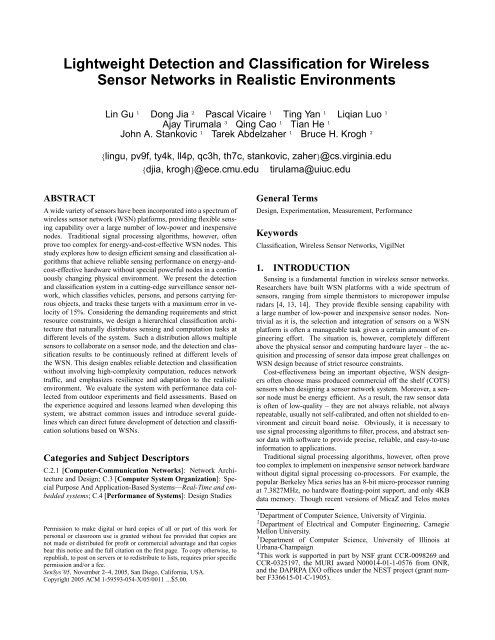
<strong>Lightweight</strong> <strong>Detection</strong> <strong>and</strong> <strong>Classification</strong> <strong>for</strong> <strong>Wireless</strong><br />
<strong>Sensor</strong> Networks in Realistic Environments<br />
ABSTRACT<br />
Lin Gu 1 Dong Jia 2 Pascal Vicaire 1 Ting Yan 1 Liqian Luo 1<br />
Ajay Tirumala 3 Qing Cao 1 Tian He 1<br />
John A. Stankovic 1 Tarek Abdelzaher 1 Bruce H. Krogh 2<br />
{lingu, pv9f, ty4k, ll4p, qc3h, th7c, stankovic, zaher}@cs.virginia.edu<br />
{djia, krogh}@ece.cmu.edu tirulama@uiuc.edu<br />
A wide variety of sensors have been incorporated into a spectrum of<br />
wireless sensor network (WSN) plat<strong>for</strong>ms, providing flexible sensing<br />
capability over a large number of low-power <strong>and</strong> inexpensive<br />
nodes. Traditional signal processing algorithms, however, often<br />
prove too complex <strong>for</strong> energy-<strong>and</strong>-cost-effective WSN nodes. This<br />
study explores how to design efficient sensing <strong>and</strong> classification algorithms<br />
that achieve reliable sensing per<strong>for</strong>mance on energy-<strong>and</strong>cost-effective<br />
hardware without special powerful nodes in a continuously<br />
changing physical environment. We present the detection<br />
<strong>and</strong> classification system in a cutting-edge surveillance sensor network,<br />
which classifies vehicles, persons, <strong>and</strong> persons carrying ferrous<br />
objects, <strong>and</strong> tracks these targets with a maximum error in velocity<br />
of 15%. Considering the dem<strong>and</strong>ing requirements <strong>and</strong> strict<br />
resource constraints, we design a hierarchical classification architecture<br />
that naturally distributes sensing <strong>and</strong> computation tasks at<br />
different levels of the system. Such a distribution allows multiple<br />
sensors to collaborate on a sensor node, <strong>and</strong> the detection <strong>and</strong> classification<br />
results to be continuously refined at different levels of<br />
the WSN. This design enables reliable detection <strong>and</strong> classification<br />
without involving high-complexity computation, reduces network<br />
traffic, <strong>and</strong> emphasizes resilience <strong>and</strong> adaptation to the realistic<br />
environment. We evaluate the system with per<strong>for</strong>mance data collected<br />
from outdoor experiments <strong>and</strong> field assessments. Based on<br />
the experience acquired <strong>and</strong> lessons learned when developing this<br />
system, we abstract common issues <strong>and</strong> introduce several guidelines<br />
which can direct future development of detection <strong>and</strong> classification<br />
solutions based on WSNs.<br />
Categories <strong>and</strong> Subject Descriptors<br />
C.2.1 [Computer-Communication Networks]: Network Architecture<br />
<strong>and</strong> Design; C.3 [Computer System Organization]: Special<br />
Purpose And Application-Based Systems—Real-Time <strong>and</strong> embedded<br />
systems; C.4 [Per<strong>for</strong>mance of Systems]: Design Studies<br />
Permission to make digital or hard copies of all or part of this work <strong>for</strong><br />
personal or classroom use is granted without fee provided that copies are<br />
not made or distributed <strong>for</strong> profit or commercial advantage <strong>and</strong> that copies<br />
bear this notice <strong>and</strong> the full citation on the first page. To copy otherwise, to<br />
republish, to post on servers or to redistribute to lists, requires prior specific<br />
permission <strong>and</strong>/or a fee.<br />
SenSys’05, November 2–4, 2005, San Diego, Cali<strong>for</strong>nia, USA.<br />
Copyright 2005 ACM 1-59593-054-X/05/0011 ...$5.00.<br />
General Terms<br />
Design, Experimentation, Measurement, Per<strong>for</strong>mance<br />
Keywords<br />
<strong>Classification</strong>, <strong>Wireless</strong> <strong>Sensor</strong> Networks, VigilNet<br />
1. INTRODUCTION<br />
Sensing is a fundamental function in wireless sensor networks.<br />
Researchers have built WSN plat<strong>for</strong>ms with a wide spectrum of<br />
sensors, ranging from simple thermistors to micropower impulse<br />
radars [4, 13, 14]. They provide flexible sensing capability with<br />
a large number of low-power <strong>and</strong> inexpensive sensor nodes. Nontrivial<br />
as it is, the selection <strong>and</strong> integration of sensors on a WSN<br />
plat<strong>for</strong>m is often a manageable task given a certain amount of engineering<br />
ef<strong>for</strong>t. The situation is, however, completely different<br />
above the physical sensor <strong>and</strong> computing hardware layer – the acquisition<br />
<strong>and</strong> processing of sensor data impose great challenges on<br />
WSN design because of strict resource constraints.<br />
Cost-effectiveness being an important objective, WSN designers<br />
often choose mass produced commercial off the shelf (COTS)<br />
sensors when designing a sensor network system. Moreover, a sensor<br />
node must be energy efficient. As a result, the raw sensor data<br />
is often of low-quality – they are not always reliable, not always<br />
repeatable, usually not self-calibrated, <strong>and</strong> often not shielded to environment<br />
<strong>and</strong> circuit board noise. Obviously, it is necessary to<br />
use signal processing algorithms to filter, process, <strong>and</strong> abstract sensor<br />
data with software to provide precise, reliable, <strong>and</strong> easy-to-use<br />
in<strong>for</strong>mation to applications.<br />
Traditional signal processing algorithms, however, often prove<br />
too complex to implement on inexpensive sensor network hardware<br />
without digital signal processing co-processors. For example, the<br />
popular Berkeley Mica series has an 8-bit micro-processor running<br />
at 7.3827MHz, no hardware floating-point support, <strong>and</strong> only 4KB<br />
data memory. Though recent versions of MicaZ <strong>and</strong> Telos motes<br />
1 Department of Computer Science, University of Virginia.<br />
2 Department of Electrical <strong>and</strong> Computer Engineering, Carnegie<br />
Mellon University.<br />
3 Department of Computer Science, University of Illinois at<br />
Urbana-Champaign<br />
4 This work is supported in part by NSF grant CCR-0098269 <strong>and</strong><br />
CCR-0325197, the MURI award N00014-01-1-0576 from ONR,<br />
<strong>and</strong> the DAPRPA IXO offices under the NEST project (grant number<br />
F336615-01-C-1905).
employ a bigger data memory, we expect the growth of computational<br />
resources on WSN plat<strong>for</strong>ms to be rather slow because of<br />
the emphasis on low power consumption, low cost, <strong>and</strong> small <strong>for</strong>m<br />
factor. Generally, resource constraints will continue to represent the<br />
reality of energy-<strong>and</strong>-cost-effective embedded systems. This strict<br />
resource limitation makes it very difficult to execute Fast Fourier<br />
Trans<strong>for</strong>mation (FFT) <strong>and</strong> other signal processing algorithms with<br />
moderate or high time/space complexity. Also, the stringent energy<br />
budget favors simple <strong>and</strong> quick algorithms over complex algorithms<br />
that require prolonged execution time.<br />
While the computation/energy resources are limited, the application<br />
requirement is not. Specifically, the development of recent<br />
surveillance WSNs requires the network to provide functionalities<br />
well beyond sensing <strong>and</strong> routing. Such surveillance WSNs are designed<br />
to detect <strong>and</strong> report certain classes of events of interest.<br />
When such an event happens, the WSN needs to detect it quickly,<br />
classify it into one category (e.g., person, vehicle), <strong>and</strong> compute its<br />
attributes (e.g., location, velocity).<br />
Designing such surveillance WSNs is a research challenge. Besides<br />
the obviously severe resource constraints, the following factors<br />
also contribute to the difficulty of the task.<br />
• To provide sensing coverage <strong>for</strong> a relatively large area, the network<br />
is usually comprised of a large number of densely deployed<br />
nodes. This imposes a challenge on efficient data propagation<br />
<strong>and</strong> reliable operation.<br />
• The detection, classification, <strong>and</strong> reporting must be per<strong>for</strong>med<br />
in a timely manner. It is usually required that the network complete<br />
the detection <strong>and</strong> classification be<strong>for</strong>e the target travels<br />
out of the field so that the system can respond to the event. As a<br />
result, offline-style processing per<strong>for</strong>med by base stations with<br />
global <strong>and</strong> relatively “complete” data is often not feasible in<br />
this context.<br />
• To per<strong>for</strong>m quality signal processing, the sensors often need to<br />
sample at a high sampling rate, stressing resource utilization.<br />
The sensing data is bursty <strong>and</strong> in large quantity.<br />
• Surveillance networks are often deployed on rough terrains <strong>for</strong><br />
a long period of time. Hence, it must be adaptive to the realistic,<br />
ever-changing environment.<br />
Given the numerous technical challenges, important research questions<br />
are: Can we construct a reliable surveillance WSN that meets<br />
the requirements within the strict resource constraints? What per<strong>for</strong>mance<br />
will such a system achieve? This study attempts to answer<br />
these questions by presenting the detection <strong>and</strong> classification<br />
system in VigilNet [10], which is a recently deployed surveillance<br />
WSN detecting <strong>and</strong> classifying vehicles, persons <strong>and</strong> persons<br />
with ferrous objects. Specifically, this paper explores the design<br />
choices involved in constructing an efficient detection <strong>and</strong> classification<br />
system that achieves reliable per<strong>for</strong>mance on a network of<br />
energy-<strong>and</strong>-cost-effective sensor nodes, analyzes the per<strong>for</strong>mance,<br />
<strong>and</strong> proposes a set of guidelines <strong>for</strong> future designs of WSNs in a<br />
similar design context.<br />
It is worth clarifying that advanced signal processing mathematics<br />
<strong>and</strong> algorithms are not the emphasis of this paper. Instead, this<br />
paper focuses on the system design issues involved in creating a<br />
reliable <strong>and</strong> realistic classification system <strong>for</strong> a surveillance WSN<br />
using homogeneously low-end sensor nodes, as well as evaluation<br />
of the effectiveness of these designs. To the authors’ best knowledge,<br />
there has not been a large-scale deployment of such a sophisticated<br />
surveillance network without using special powerful nodes.<br />
Hence, our study is focused on answering this challenge: Without<br />
enhancing any individual nodes’ capability <strong>and</strong> cost, can a network<br />
of distributed sensor nodes provide advanced functions <strong>and</strong> work<br />
reliably in realistic environments? We believe that the experience<br />
acquired <strong>and</strong> lessons learned in constructing such a system, <strong>and</strong> the<br />
analysis of the trade-offs <strong>and</strong> design decisions in it, will benefit the<br />
research in this area, <strong>and</strong> help trans<strong>for</strong>m the research potential of<br />
WSNs into real-world technology <strong>and</strong> market success.<br />
The paper is organized as follows. Section 2 presents background<br />
in<strong>for</strong>mation <strong>and</strong> surveys related work. Section 3 gives an<br />
overview of the VigilNet surveillance system. Section 4 presents<br />
the design of the hierarchical classification architecture. System<br />
level evaluation is shown in Section 5. Section 6 discusses several<br />
guidelines <strong>for</strong> designing a large-scale WSN <strong>for</strong> detection <strong>and</strong><br />
classification tasks. Finally, Section 7 concludes the paper.<br />
2. BACKGROUND<br />
Focusing on VigilNet’s hardware plat<strong>for</strong>m, we present a brief<br />
overview of the sensing subsystem – sensors <strong>and</strong> their supporting<br />
circuitry – on a sensor node. The sensing subsystem is the hardware<br />
foundation on which classification systems are constructed.<br />
We also survey the related work in the area of detection <strong>and</strong> classification<br />
WSN systems.<br />
2.1 Overview of the sensing subsystem<br />
VigilNet uses the ExScal motes as sensor nodes. Based on the<br />
Mica2 [3] mote design, the ExScal mote, shown in Fig. 1, is designed<br />
by CrossBow Inc. <strong>and</strong> Ohio State University <strong>for</strong> large-scale<br />
surveillance WSNs [8]. The major difference between the ExScal<br />
mote <strong>and</strong> the Berkeley Mica2 mote is that the <strong>for</strong>mer integrates<br />
a magnetometer (Honeywell HMC1052[2]), a microphone, <strong>and</strong> 4<br />
PIR sensors on the same circuit board as the processor’s. After the<br />
first prototype ExScal motes were delivered in March 2004, Cross-<br />
Bow released several versions with various improvements throughout<br />
the year of 2004.<br />
Several correlated factors contribute to the complexity of the<br />
sensing circuitry. First, applications require a long sensing distance,<br />
which implies a finer granularity <strong>for</strong> the sensor readings.<br />
Second, as a general purpose plat<strong>for</strong>m, designers hope to choose<br />
sensors with a wide measuring range. Third, the wider measuring<br />
range combined with a finer granularity maps to more numeric values<br />
which, however, have to all fall into the representation capability<br />
of the A/D converter (ADC), I/O bus, <strong>and</strong> CPU I/O port width.<br />
Finally, as the sensors on the sensor board grow in both number <strong>and</strong><br />
sophistication, the support circuitry may need to support better filtering,<br />
h<strong>and</strong>le more advanced signaling protocols, employ a faster<br />
or wider bus, provide wider functionality (such as waking up the<br />
sensor node), or build better shielding to avoid cross-talk among<br />
various components. These factors make the design of the sensing<br />
subsystem a significant engineering ef<strong>for</strong>t involving numerous<br />
design choices which often depend on the application domain.<br />
Figure 1: ExScal mote<br />
sor <strong>and</strong> sensor components.<br />
To solve the a<strong>for</strong>ementioned<br />
range <strong>and</strong> granularity problems <strong>for</strong><br />
the magnetometer, the ExScal mote<br />
includes circuitry that allows the<br />
application program to adjust the<br />
input signal to be amplified. To<br />
provide a quality signal <strong>for</strong> acoustic<br />
processing, the microphone circuitry<br />
incorporates a high-pass filter<br />
<strong>and</strong> a low-pass filter. Both the<br />
input adjustment <strong>and</strong> filtering are<br />
controllable by the processor, with<br />
an I 2 C bus connecting the proces
2.2 Related work<br />
With the development of WSN systems, sensing, detection, <strong>and</strong><br />
tracking have been a prosperous research area. Specifically, Wang<br />
et. al. studied acoustic tracking using Mica motes [22]. Simon<br />
et. al. designed a sniper localization system with acoustic signal<br />
processing [19] <strong>and</strong> accomplished good per<strong>for</strong>mance. Different<br />
from VigilNet’s homogeneous approach, these systems employ<br />
special powerful nodes or DSP co-processors to process acoustic<br />
data. Zhao et. al. described collaborative signal processing [25]<br />
to retrieve more accurate in<strong>for</strong>mation from sensor data <strong>and</strong> achieve<br />
better target tracking per<strong>for</strong>mance. Pattem et. al. build a framework<br />
to evaluate the tracking strategies in an energy aware context<br />
[18]. Most of the per<strong>for</strong>mance analysis in [25] <strong>and</strong> [18] are conducted<br />
by simulations, concentrating on exploring the design space<br />
<strong>and</strong> trade-offs under specific constraints <strong>and</strong> assumptions.<br />
Along the direction of real-world application <strong>and</strong> deployments,<br />
researchers have also constructed a number of successful systems.<br />
Szewczyk et. al. [21] developed a habitat monitoring WSN on the<br />
Great Duck Isl<strong>and</strong> <strong>and</strong> the system operated <strong>for</strong> months. Zhang et.<br />
al. developed a WSN <strong>for</strong> wild life tracking [24]. These systems<br />
demonstrate the flexibility <strong>and</strong> capability of the WSN technology<br />
in various applications. However, VigilNet faces more dem<strong>and</strong>ing<br />
application requirements. As a result, many design choices are<br />
different in these systems than in VigilNet. For example, many current<br />
systems typically employ centralized processing which is not<br />
feasible in many surveillance networks [7].<br />
In [11], the authors describe a surveillance network that can detect<br />
moving targets. The system uses Mica2 motes [3] equipped<br />
with a magnetometer (Honeywell HMC1002 [2]), an acoustic sensor<br />
<strong>and</strong>, on some nodes, a motion sensor. The motion sensor is an<br />
Advantaca MIR (micropower impulse radar) sensor which transmits<br />
microwave signals <strong>and</strong> detects motion by capturing distortion<br />
of the reflected signal. The network reports a target as a walking<br />
person or a vehicle. There<strong>for</strong>e, it has a preliminary classification<br />
capability. However, there is very limited signal processing in it.<br />
As a result, the classification is limited in both functionality <strong>and</strong><br />
per<strong>for</strong>mance. Also, the MIR sensors, worth four thous<strong>and</strong> dollars<br />
each, are not a typical choice <strong>for</strong> energy-<strong>and</strong>-cost-effective systems.<br />
Brooks et. al. [7] introduced a collaborative signal processing<br />
framework <strong>for</strong> sensor networks using location-aware routing <strong>and</strong><br />
collaborative signal processing. Their study provides many insights<br />
into the distributed collaborative classification in WSNs. Nevertheless,<br />
the CSP framework involves non-trivial training <strong>and</strong> computation<br />
overhead, which our system cannot af<strong>for</strong>d. Also, the system<br />
implementation <strong>and</strong> evaluation of the CSP framework employ<br />
nodes with higher power than the energy-<strong>and</strong>-cost-effective WSN<br />
nodes our system is targeting. In fact, VigilNet must satisfy three<br />
conflicting requirements simultaneously – low-end hardware, long<br />
lifetime, <strong>and</strong> sophisticated function. This challenging design context<br />
is different than what past solutions assume.<br />
Among recently deployed WSNs, the Extreme Scaling project is<br />
the most similar to VigilNet in functionality <strong>and</strong> hardware plat<strong>for</strong>m<br />
[1, 8]. However, a major difference is that the Extreme Scaling<br />
WSN employs a heterogeneous network topology <strong>and</strong> uses a more<br />
powerful Stargate node <strong>for</strong> some computation <strong>and</strong> communication<br />
intensive tasks.<br />
3. OVERVIEW OF THE DETECTION AND<br />
CLASSIFICATION IN VIGILNET<br />
The VigilNet surveillance system [5] is a WSN with 200 sensor<br />
nodes (ExScal motes). The WSN is required to per<strong>for</strong>m timely detection,<br />
tracking <strong>and</strong> classification of vehicles, persons, <strong>and</strong> persons<br />
Figure 2: Screen of tracking a person with ferrous objects<br />
with ferrous objects. When a target is detected, the WSN reports<br />
the detection to an external device. The external device can be<br />
a more powerful sensor, a communication device connecting to a<br />
control center, or any device that h<strong>and</strong>les the in<strong>for</strong>mation delivered<br />
by the WSN. A base mote connects to the external device through<br />
a UART interface, <strong>and</strong> serves as a router between the WSN <strong>and</strong><br />
the external device. As the target travels in the network, the WSN<br />
garners enough in<strong>for</strong>mation to classify the target <strong>and</strong> compute its<br />
attributes, such as location <strong>and</strong> velocity, <strong>and</strong> the results are delivered<br />
to the external device as periodic updates. Fig. 2 shows a<br />
screen snapshot of VigilNet deployed along two roads <strong>for</strong>ming a<br />
“T” shape. It illustrates the detection <strong>and</strong> classification of a “person<br />
with ferrous objects” target. Moreover, the WSN is to be deployed<br />
in a rough terrain <strong>and</strong> operate <strong>for</strong> months. Hence, the detection <strong>and</strong><br />
classification algorithms must be adaptive to environmental variety<br />
<strong>and</strong> weather changes.<br />
As in many surveillance systems, VigilNet emphasizes that the<br />
false negative rate (the possibility of a target not being detected)<br />
must be very low. Meanwhile, it also requires a low false positive<br />
rate (the possibility of an event being reported without a real<br />
target in the field) since false positives waste energy <strong>and</strong> reduce<br />
the overall system lifetime. This implies that the wake-up (most<br />
of the network nodes are in sleep mode when there are no events<br />
of interest), sensing <strong>and</strong> classification must complete within a time<br />
constraint. These two factors – energy efficiency <strong>and</strong> low latency<br />
– make it undesirable to have a centralized semi-offline algorithm<br />
that collects all data from the network, transports them to a base<br />
station, <strong>and</strong> lets a powerful node analyze data <strong>and</strong> per<strong>for</strong>m classification.<br />
Instead, the network, including the base mote (also an<br />
energy-<strong>and</strong>-cost-effective device), must per<strong>for</strong>m reliable detection<br />
<strong>and</strong> classification functions independently in a timely manner without<br />
powerful nodes involved.<br />
To build a complete VigilNet <strong>for</strong> realistic outdoor environments,<br />
other middleware services are also integrated. In brief, the localization<br />
is done through the walking GPS solution [20], which assigns<br />
nodes their location at the time they are deployed. The time<br />
synchronization used in VigilNet is a variation of the FTSP protocol<br />
[17] without periodic adjustments <strong>for</strong> the sake of stealthiness.<br />
Routing infrastructure is a set of multi-parent diffusion trees (<strong>for</strong>est)<br />
rooted at the base nodes. To achieve long-term surveillance, a<br />
multi-dimensional power management scheme is proposed in [12].<br />
In this paper, we focus on the design of the detection <strong>and</strong> classification<br />
system in VigilNet, which is not addressed in other papers, but<br />
is a major part of the system <strong>and</strong> directly determines the system’s<br />
functionality <strong>and</strong> per<strong>for</strong>mance.
4. CLASSIFICATION SYSTEM DESIGN<br />
In this section, we present the design of the classification architecture,<br />
including the sensing algorithms <strong>for</strong> the magnetometer,<br />
motion sensor, <strong>and</strong> microphone (acoustic sensor).<br />
We call the sensor reading at a specific time on a specific sensor<br />
on a specific node a sample point. When a sensor network starts<br />
operation, each sensor on each node in the network produces a sequence<br />
of sample points. All the sample points produced by the<br />
network <strong>for</strong>m a set <strong>and</strong> we call it the global sample set.<br />
The global sample set is the complete in<strong>for</strong>mation about what<br />
happens in the network. If all the nodes report their sample points<br />
to a base station, the base station can collect the global sample set<br />
<strong>and</strong> per<strong>for</strong>m computation with it. This solution has been successfully<br />
used in a number of WSNs. For surveillance WSNs, however,<br />
this is often not feasible because it is too expensive to collect the<br />
global sample set in a sensor network. As an example, a 150-node<br />
habitat monitoring WSN, presented in [21], collected temperature,<br />
humidity, <strong>and</strong> barometric pressure sensor readings <strong>and</strong> routed them<br />
back to base stations <strong>for</strong> analysis. During its 115 days of operation,<br />
the network collected <strong>and</strong> routed 650,000 observations. In<br />
VigilNet, the data <strong>for</strong> a one-minute target detection <strong>and</strong> classification<br />
event, with 200 nodes <strong>and</strong> acoustic processing, well exceeds<br />
1,000,000 observations. If targets enter the network once a day <strong>and</strong><br />
we routed all the data (the global sample set) back to the base mote,<br />
the system could hardly last a week. Hence, the “sense-store-send”<br />
style processing is not suitable <strong>for</strong> latency-sensitive surveillance<br />
systems that require a high sampling rate.<br />
On the other h<strong>and</strong>, the sequence of sample points on a single<br />
node does not have enough in<strong>for</strong>mation to support reliable detection<br />
<strong>and</strong> classification. As an example, a transient disturbance (such<br />
as a curious bird l<strong>and</strong>ing on the sensor) may shake the node <strong>and</strong><br />
trigger PIR <strong>and</strong> magnetic detections. Individual sensor nodes cannot<br />
distinguish such an unexpected event from a moving person<br />
with ferrous objects. Generally, observations on an individual node<br />
are not a reliable indication of events in a network.<br />
Hence, we must design the detection <strong>and</strong> classification system<br />
so that the sensing <strong>and</strong> classification functions are reasonably distributed<br />
in the network <strong>and</strong> the sensor nodes can cooperate to detect<br />
target signatures, reduce false positives, <strong>and</strong> achieve reliable<br />
<strong>and</strong> timely classification at reasonable energy cost. This motivates<br />
us to choose a hierarchical architecture <strong>for</strong> the classification system.<br />
In fact, the concept of hierarchical processing is not new in<br />
WSNs. The unique characteristics of our hierarchical design are<br />
in the organization of various components <strong>and</strong> the distribution of<br />
the detection <strong>and</strong> classification tasks in such a hierarchy so that<br />
the system accomplishes the required per<strong>for</strong>mance with minimal<br />
overhead. Illustrated in Fig. 3, the hierarchical classification architecture<br />
is comprised of four tiers – sensor-level, node-level, grouplevel,<br />
<strong>and</strong> base-level. The classification result is represented by a<br />
data structure called the confidence vector. The confidence vector<br />
comprises the confidence levels <strong>for</strong> the corresponding targets,<br />
<strong>and</strong> is used as a common data structure to transport in<strong>for</strong>mation<br />
between different levels of the classification hierarchy.<br />
The lowest level deals with individual sensors <strong>and</strong> comprises the<br />
sensing algorithms <strong>for</strong> the corresponding sensors. With communication<br />
being a costly operation, the sensing algorithms need to<br />
per<strong>for</strong>m local detection <strong>and</strong> classification as much as possible. After<br />
processing the sensor data, each sensing algorithm delivers the<br />
confidence vector to the higher level module – the node-level detection<br />
<strong>and</strong> classification module.<br />
The node-level classification deals with output from multiple<br />
sensors on the node. The fusion of the data from various sensors<br />
exposes more useful in<strong>for</strong>mation than can be obtained from any in-<br />
Group<br />
Group<br />
Group leader, per<strong>for</strong>ming<br />
group -level classification<br />
Normal mote, per<strong>for</strong>ming sensor<br />
<strong>and</strong> node -level classification<br />
Ba se mo te, per <strong>for</strong>mi ng<br />
base -level classification<br />
Group<br />
Figure 3: Hierarchical <strong>Classification</strong> Architecture<br />
dividual sensor. Hence, the node-level sensing algorithm must correlate<br />
the sensor data from individual sensors <strong>and</strong> <strong>for</strong>m node-level<br />
classification results. Such a correlation can enhance the detection<br />
<strong>and</strong> classification accuracy on individual nodes – different sensors<br />
may strengthen the confidence of each other’s classification results<br />
<strong>and</strong> invalidate false positives. Furthermore, the node-level classification<br />
module monitors the sensors’ status <strong>and</strong> per<strong>for</strong>ms sanity<br />
control over sensors. For example, it detects <strong>and</strong> shuts down faulty<br />
sensors. Though these functions are all important aspects in the hierarchical<br />
classification architecture, this paper does not detail the<br />
design of the node-level classification because, compared to other<br />
components, it is not the challenging part in the system.<br />
The sensor-level <strong>and</strong> node-level classification functions both reside<br />
on a single node. The level above, the group-level classification,<br />
is per<strong>for</strong>med by groups of nodes. Such groups are managed<br />
by a middleware called EnviroSuite [15], which provides a<br />
set of distributed group management protocols to dynamically organize<br />
nodes in the vicinity of targets into groups <strong>and</strong> elect leaders<br />
among them. These leaders are designated to collect the node-level<br />
classification results from individual members <strong>and</strong>, based on them,<br />
per<strong>for</strong>m the group-level classification. Thus, the input to the grouplevel<br />
classification is the node-level confidence vectors rather than<br />
a bulk of sample points. This greatly reduces the volume of in<strong>for</strong>mation<br />
transmitted between group leaders <strong>and</strong> members. Group<br />
leaders have much better views of targets compared with individual<br />
nodes. There<strong>for</strong>e, besides group-level classification they are<br />
able to execute more complicated tasks which are extremely hard<br />
or even impossible <strong>for</strong> the node-level. Examples include suspicious<br />
report/node detection (based on spacial <strong>and</strong> temporal correlations<br />
among members) <strong>and</strong> aggregate attribute computation (e.g., computing<br />
average member locations as estimates of target positions).<br />
The highest level in the hierarchical classification architecture is<br />
the base-level classification. The group-level classification results<br />
are transported via multiple hops to the base mote, serving as the<br />
input to the base-level classification algorithm. The base-level classification<br />
algorithm finalizes the sensing <strong>and</strong> classification result, as<br />
well as computing attributes (e.g., velocity) of the event.<br />
In the following subsections, we present sensing algorithms <strong>for</strong><br />
the magnetometer, the motion sensor, <strong>and</strong> the acoustic sensor, focusing<br />
on their unique characteristics. Some techniques are used in<br />
more than one sensing algorithm. To avoid redundancy, we present<br />
them in the sensing algorithm where their purpose <strong>and</strong> effects can<br />
be most clearly explained. In Section 4.4 <strong>and</strong> 4.5, we describe the<br />
group-level <strong>and</strong> base-level classification, respectively.<br />
4.1 Sensing Algorithm <strong>for</strong> Magnetometer<br />
In VigilNet, the requirement <strong>for</strong> magnetic sensing is to detect<br />
vehicles <strong>and</strong> persons with ferrous objects. Since the magnetometer
circuitry in the ExScal mote senses a wide range of signals with<br />
a fine granularity, we can use it to measure deflection of the magnetic<br />
field caused by motion of ferrous objects (e.g., vehicles or<br />
weapons). Straight<strong>for</strong>ward as it looks, challenges abound in designing<br />
a reliable magnetic sensing algorithm <strong>for</strong> the low-power<br />
sensor network plat<strong>for</strong>m.<br />
First, raw ADC readings easily saturate due to the a<strong>for</strong>ementioned<br />
granularity/range problem. The ADC on the ExScal plat<strong>for</strong>m<br />
is 10 bits wide, representing 1024 values. But the wide range<br />
of signal intensity combined with a fine granularity requires a much<br />
larger value set than the available 0 to 1023. Second, the response<br />
latency is too long <strong>for</strong> accurate signal wave<strong>for</strong>m extraction. The<br />
magnetometer circuitry needs about 40 milliseconds to stabilize,<br />
<strong>and</strong> each tuning of the potentiometer needs about 50 milliseconds<br />
to stabilize. Third, electromagnetic noise from the circuit board<br />
lowers the S/N ratio <strong>and</strong> imposes serious problems on the magnetic<br />
sensing algorithm to distinguish signals from noise. Fourth, thermal<br />
drift is a severe issue – When the ambient temperature changes,<br />
the sensor readings change accordingly. Finally, radio transmission<br />
interferes with the magnetometer sensing circuit.<br />
Among the five issues, the response time is a hardware characteristic.<br />
We cannot eliminate such delays. Instead, we measure<br />
such delays <strong>and</strong> reduce them to as low as safety allows. The radio/magnetometer<br />
interference can be solved by scheduling the radio<br />
<strong>and</strong> magnetometer to work in separate time slots. The other<br />
three issues are more interesting research questions with practical<br />
importance to a number of amplitude based sensors. Hence, Section<br />
4.1.1 discusses the sensor reading <strong>and</strong> signal/noise ratio, <strong>and</strong><br />
Section 4.1.2 discusses how to deal with the thermal drift. We also<br />
use the magnetic sensing algorithm as an example to discuss the<br />
trade-off between sensitivity <strong>and</strong> resilience in Section 4.1.3.<br />
4.1.1 Mag-Points<br />
As mentioned above, raw ADC readings are not suitable to represent<br />
the magnetic field intensity, <strong>and</strong> the magnetometer suffers<br />
from a low signal/noise ratio. Both issues relate to a basic question:<br />
how to provide credible sensor readings with semantics that<br />
higher-level signal processing algorithms can easily use? Hence,<br />
we h<strong>and</strong>le these two issues together, by trans<strong>for</strong>ming the the raw<br />
sensor reading into a 32-bit uni<strong>for</strong>m measure, the Mag-Point.<br />
First, the sensing algorithm trans<strong>for</strong>ms the raw ADC reading into<br />
a scaled ADC reading. The numeric value of the raw ADC reading<br />
(r) is determined by the voltage across the magnetic signal line<br />
<strong>and</strong> a reference line. The voltage on the reference line is determined<br />
by a digital potentiometer setting. By studying the relation<br />
of the changes of potentiometer value (p) with the changes of ADC<br />
reading, we map the potentiometer value into certain ADC units.<br />
On ExScal motes, experiments reveal that 1 unit of potentiometer<br />
change equals 210 ADC units. At run time, as the magnetic signal<br />
varies, the sensing algorithm dynamically searches <strong>and</strong> sets the potentiometer<br />
to adjust the reference voltage to a suitable level, <strong>and</strong><br />
combines r <strong>and</strong> p to acquire scaled ADC readings (s) using the<br />
linear <strong>for</strong>mula: s = 210 · p + r<br />
Then, the sensing algorithm averages scaled ADC readings to<br />
acquire Mag-Points, using the following moving average<br />
0 = s0<br />
n = αmp · sn + (1 − αmp)<br />
n−1<br />
Here n is the n th Mag-Point, <strong>and</strong> sn is the n th scaled ADC reading.<br />
The process of generating Mag-Points from raw magnetometer<br />
signals filters out high frequency noise <strong>and</strong> the results are relatively<br />
reliable measures representing the current magnetic field intensity.<br />
As a comparison, Fig. 4(a) shows the wave<strong>for</strong>m of raw magnetic<br />
signals (scaled ADC readings) sampled at 32Hz when an iron bar<br />
moved at 5 feet away. As we can see, the signals of the moving iron<br />
bar are hidden in high noise.<br />
In contrast, Fig. 4(b) shows the wave<strong>for</strong>m of the Mag-Points,<br />
with αmp = 1/18, <strong>for</strong> the same target. The signal is more evident<br />
with Mag-Points, which filters out a large part of the noise. There<strong>for</strong>e,<br />
the Mag-Point is not only a uni<strong>for</strong>m numeric value that is easy<br />
to use, but also a loyal indication of the magnetic field intensity that<br />
higher-level algorithms can rely on. Such a low-complexity technique<br />
is applicable to many amplitude based signals.<br />
Reading<br />
22000<br />
20000<br />
18000<br />
16000<br />
14000<br />
12000<br />
10000<br />
8000<br />
6000<br />
Scaled ADC reading<br />
500 1000 1500 2000<br />
Sample<br />
(a) Scaled ADC readings<br />
Reading<br />
18000<br />
17000<br />
16000<br />
15000<br />
14000<br />
13000<br />
12000<br />
11000<br />
10000<br />
Mag Point<br />
1500 2000 2500 3000 3500<br />
Sample<br />
(b) Mag-Point readings<br />
Figure 4: Scaled ADC readings <strong>and</strong> Mag-Points collected from<br />
the same sensor in two consecutive runs<br />
4.1.2 Thermal Drift<br />
Thermal drift is the most difficult noise the sensing algorithm<br />
needs to filter out. Fig. 5(a) shows the magnetometer observations<br />
on the X-axis when a sensor node was moved from an airconditioned<br />
room to outdoors on a sunny day. The Mag-Point readings,<br />
sampled at 32Hz, fluctuated <strong>and</strong> dropped quickly in about<br />
15 seconds. Sometimes, the thermal drift is identical to a ferrous<br />
target. Fig. 5(b) shows readings collected at noon on a cloudy<br />
<strong>and</strong> windy day. The sensor node was an ExScal mote version 1,<br />
which has no enclosure. The frequent alternations of sunshine <strong>and</strong><br />
shadow caused the temperature of the exposed magnetometer to<br />
change quickly. Note that the readings from 300 to 500 (about 6<br />
seconds) is similar to a car moving slowly. Such an intrinsically<br />
ambiguous thermal drift cannot be filtered out algorithmically. In<br />
such situations, other measures must be employed to avoid such<br />
ambiguity. Packaging is the most important supplementary factor<br />
that ensures that thermal drift does not produce ambiguous signal<br />
wave<strong>for</strong>ms.<br />
Assuming intrinsically ambiguous thermal drifts are eliminated<br />
by methods other than software, frequency based analysis can be<br />
used to filter out other thermal drifts. The thermal drift is a relatively<br />
slow change, i.e., low frequency noise. To eliminate this,<br />
the sensing algorithm uses another moving average, which assigns<br />
more weight on history, to compute the current base signal line.<br />
The <strong>for</strong>mula <strong>for</strong> Bn (the nth point in the base signal line) is<br />
B0 = s0<br />
Bn = αB · sn + (1 − αB) · Bn−1<br />
Fig. 5(a) also shows the base signal line. As we may notice, when<br />
the sensor readings change, the base signal line readings change at<br />
a slower speed than the Mag-Points. When the Mag-Points deviate<br />
from the base signal line <strong>for</strong> an amount larger than a threshold,<br />
detection occurs.<br />
By using two moving averages with very low computational complexity,<br />
the magnetic sensing algorithm filters out both high frequency<br />
<strong>and</strong> low frequency noise, solves the problems of non-uni<strong>for</strong>m
Reading<br />
Reading<br />
5000<br />
4500<br />
4000<br />
3500<br />
3000<br />
2500<br />
Mag Point<br />
Base Line<br />
2000<br />
300 350 400 450 500 550 600 650 700 750 800<br />
Sample<br />
(a) Readings as temperature increases<br />
65000<br />
60000<br />
55000<br />
50000<br />
45000<br />
40000<br />
35000<br />
Mag-Point readings<br />
30000<br />
0 200 400 600 800 1000<br />
Sample<br />
(b) Readings on a cloudy <strong>and</strong> windy day<br />
Figure 5: The impact of temperature on the magnetometer<br />
sensor reading, low signal/noise ratio, <strong>and</strong> thermal drift, <strong>and</strong> accomplishes<br />
a resilient detection algorithm.<br />
4.1.3 Trade-off between sensitivity <strong>and</strong> resilience<br />
The parameters αmp <strong>and</strong> αB affect the per<strong>for</strong>mance of the magnetic<br />
sensing <strong>and</strong> must be carefully chosen so that the magnetic<br />
sensing algorithm is not only sensitive, but also resilient to noise<br />
<strong>and</strong> environmental changes.<br />
The parameter αmp affects how effectively the algorithm averages<br />
out high frequency noise. If αmp = 1, there is no noise filtering.<br />
As we decrease αmp, high frequency noise is filtered out by<br />
the averaging process, <strong>and</strong> small signals are able to emerge from the<br />
background noise. When αmp approaches 0, however, the history<br />
readings overwhelm the new reading so much that signals lasting<br />
<strong>for</strong> a short period of time cannot distinguishably change the Mag-<br />
Point readings. Hence, the algorithm becomes unable to detect a<br />
target unless it is moving very slowly. This means that the sensitivity<br />
decreases, <strong>and</strong> the false negative rate increases, when αmp is<br />
too large, or too small.<br />
The parameter αB aims to establish a baseline to characterize the<br />
ambient magnetic field strength without targets. If αB = αmp, the<br />
baseline reading Bn is the same as the Mag-Point<br />
n, <strong>and</strong> there<br />
can be no detection since their difference is always 0. With αmp<br />
fixed <strong>and</strong> αB decreasing, the baseline becomes more stable. When<br />
a target approaches, the Mag-Points change faster than the baseline.<br />
Generally, the smaller the αB, the larger the difference between the<br />
baseline <strong>and</strong> Mag-Points, <strong>and</strong> the more sensitive the magnetic algorithm<br />
is. However, when αB increases, the baseline also becomes<br />
less adaptive to environmental changes, such as the temperature<br />
change, <strong>and</strong> becomes more likely to report false positives. When<br />
αB = 1, the algorithm has the maximum sensitivity, but shows a<br />
very weak resilience because it does not adapt to the environment at<br />
all <strong>and</strong> thus any environmental change can trigger a false positive.<br />
As we can see from the analysis above, choosing a suitable αmp<br />
<strong>and</strong> αB is a design decision that affects the magnetic sensing algorithm’s<br />
per<strong>for</strong>mance. Their ranges of suitable values are dependent<br />
on the application requirements, the sensor properties, <strong>and</strong><br />
the expected environmental variability. In VigilNet, we choose<br />
αmp = 1/4 <strong>and</strong> αB = 1/64, after weighing the above factors<br />
<strong>and</strong> experimenting with a number of settings.<br />
4.2 Sensing Algorithm <strong>for</strong> Motion <strong>Sensor</strong>s<br />
The task <strong>for</strong> motion sensors is to detect movement of an object<br />
in the region where the sensor network is deployed. The motion<br />
sensors on sensor boards are peroelectric infra-red (PIR) sensors.<br />
They sense changes in the thermal field over the region. During<br />
the time when an object is moving through, the variations of the<br />
thermal field result in unbalanced infra-red signals detected by the<br />
lens pairs in the PIR sensor, leading to positive detections. Unlike<br />
the magnetometer, the PIR signals are AC signals, not amplitude<br />
based. A distinctive challenge to designing a reliable motion<br />
sensing algorithm is the weather. Hence, we introduce a motion<br />
sensing algorithm, focusing on its low-complexity frequency based<br />
processing <strong>and</strong> environmental resilience.<br />
4.2.1 Increasing S/N ratio by filters<br />
In outdoor environments, the per<strong>for</strong>mance of PIR sensors depends<br />
heavily on the weather conditions, including wind, temperature<br />
<strong>and</strong> humidity. Wind makes the air move <strong>and</strong> grass <strong>and</strong> trees<br />
swing, causing the thermal field to change since the air temperature<br />
is not uni<strong>for</strong>m <strong>and</strong> grass <strong>and</strong> trees have different temperatures. Fig.<br />
6(a) shows PIR data collected by a sensor in grass on a hot, humid<br />
<strong>and</strong> windy day <strong>and</strong> Fig. 6(b) is the spectrum of the signal. There is<br />
a moving target in the area between 60s <strong>and</strong> 70s. On hot, humid <strong>and</strong><br />
windy days, when the sensors are placed in grass, a simple energy<br />
detector either generates false positives, if using a low threshold, or<br />
misses targets, if using a high threshold. We observe that the low<br />
frequency component, less than 1 Hz, dominates the noise. When<br />
a target moves through, the frequency components larger than 2Hz<br />
become significant. This motivates us to explore frequency based<br />
signal processing on PIR data.<br />
Because of the limited computation resource <strong>and</strong> the time constraints<br />
of the application, we design a high pass filter as follows.<br />
0 = 0<br />
n = sn − sn−1 + 0.9<br />
n−1<br />
Fig. 7(a) shows the frequency response of the filter. Fig. 7(b) shows<br />
the spectrum of filtered PIR data on a hot <strong>and</strong> windy day collected<br />
by a sensor in grass. The coefficient 0.9 is decided empirically with<br />
different filters on PIR data collected outdoors. Although a higher<br />
order filter could achieve lower gain <strong>for</strong> components less than 1 Hz,<br />
it does not significantly improve the per<strong>for</strong>mance.<br />
Fig. 8(a) is the filtered signal of the one in Fig. 6(a). When the<br />
moving object passes, there is considerable energy variation in the<br />
signal. A simple energy detector can then be applied to the filtered<br />
signal to detect movements with a low false positive rate.<br />
4.2.2 Unsupervised adaptation to environment<br />
In the motion sensing algorithm, the energy based target detection<br />
threshold must be set based on the noise level. However, in realistic<br />
environments, the noise level is not fixed. The low frequency<br />
noise is very weak on cold <strong>and</strong> arid days, but can be strong on hot<br />
<strong>and</strong> windy days. Fig. 8(a) <strong>and</strong> Fig. 8(b) compare the PIR data <strong>for</strong><br />
two different scenarios. Obviously, we cannot achieve good per<strong>for</strong>mance<br />
with a fixed threshold in all types of weather conditions.<br />
To solve this problem, we use an unsupervised adaptation tech-
PIR Reading (unit)<br />
1200<br />
1000<br />
800<br />
600<br />
400<br />
200<br />
0<br />
0 20 40 60 80 100 120<br />
Time (second)<br />
(a) PIR data<br />
(b) Spectrum of PIR data<br />
Figure 6: PIR readings from sensor in grass<br />
nique to adjust the threshold. The sensors continuously compute<br />
the noise level based on local measurements <strong>and</strong> adapt the threshold<br />
proportional to the noise level. To compute the noise level, the<br />
motion sensing algorithm monitors the maximum power pn of the<br />
filtered signal within a time window. The noise level ɛn is updated<br />
by the following computation.<br />
ɛn ¡¢ p0<br />
=<br />
n = 0<br />
0.98ɛn−1 + 0.02pn ɛn−1 < pn<br />
0.75ɛn−1 + 0.25pn ɛn−1 ≥ pn<br />
The motivation of this <strong>for</strong>mula is to let ɛn increase <strong>and</strong> decrease<br />
at different speeds. This is because the weather changes slowly<br />
there<strong>for</strong>e we don’t need to increase the noise level quickly to adapt<br />
to the weather change. A small weight on pn <strong>for</strong> pn > ɛn−1 avoids<br />
the identified noise level increasing too fast when there are moving<br />
targets. Once there is no target, we decrease the noise level quickly<br />
with large weight on pn <strong>for</strong> pn ≤ ɛn−1. Fig. 9(a) shows the signal<br />
power of filtered PIR data in Fig. 8(a). The dashed curve is the<br />
identified noise level <strong>and</strong> the dashed-dotted curve is the updated<br />
threshold that is 1.5ɛn. An exceptionally large noise after 80 seconds<br />
causes a false detection.<br />
The motion sensing algorithm monitors the number of detections<br />
within a time window <strong>and</strong> defines the percentage of the detection<br />
within the time window to be the confidence of a target in the field.<br />
Fig. 9(b) shows the sensor confidence <strong>for</strong> the signal in Fig. 6(a).<br />
4.3 Sensing Algorithm <strong>for</strong> Microphone<br />
VigilNet uses acoustic sensing to differentiate between vehicles<br />
<strong>and</strong> humans. Acoustic sensing is unique in its relatively high frequency<br />
in sampling <strong>and</strong> processing. The resource constraints make<br />
it challenging to design a reliable acoustic sensing algorithm. First,<br />
the simultaneous use of magnetic <strong>and</strong> motion sensing limits the<br />
Frequency Response<br />
10 0<br />
10 −1<br />
10 −1<br />
10 0<br />
10 1<br />
Frequency (Hz)<br />
(a) Frequency response<br />
(b) Spectrum(filtered data)<br />
Figure 7: PIR data filter<br />
rate at which we can collect acoustic samples. Second, the CPU<br />
must remain available at all times to process incoming messages.<br />
Third, the system must continuously process acoustic data in order<br />
to detect <strong>and</strong> identify targets in time. Fourth, our whole surveillance<br />
system only has 4KB RAM <strong>for</strong> its functioning: our acoustic<br />
algorithm should occupy as little memory as possible.<br />
Frequency analysis could be an effective method to conduct acoustic<br />
detection <strong>and</strong> classification. Un<strong>for</strong>tunately, computing the frequency<br />
spectrum by FFT <strong>and</strong> analyzing the spectrum are expensive<br />
operations in our design context. The number of multiplications<br />
it takes to get the frequency domain results is Θ(N log 2 N). The<br />
microcontroller ATmega128L used in the Mica2 <strong>and</strong> ExScal motes<br />
does not support native floating-point multiplication <strong>and</strong> the clock<br />
rate is between 4 MHz to 8 MHz. Xu shows that in [23], it takes<br />
a Mica mote with a 4MHz processor 30 seconds to finish a 512point<br />
FFT. Hence, an ExScal mote with a similar processor runs 15<br />
seconds <strong>for</strong> a 512-point FFT even if it is running at its maximum 8<br />
MHz clock rate. Such a long latency is not acceptable in our application.<br />
The space complexity is another issue. Although there are<br />
in-place fixed-point FFT solutions, even when we consider a 1024point<br />
FFT <strong>and</strong> each data point is 16 bit, an in-place solution still<br />
uses at least 2 KB space just <strong>for</strong> the data points. In order to save<br />
the 16-bit trigonometric value table, which is necessary <strong>for</strong> FFT<br />
calculation, another 2 KB is needed. In Mica/Mica2 series motes,<br />
the RAM size is 4KB <strong>and</strong> a large proportion of the RAM needs to<br />
be assigned to other modules. Of course, the off-chip Flash can be<br />
used as secondary storage, but frequent writes to the Flash makes<br />
the FFT computation even slower <strong>and</strong> quickly damage the Flash.<br />
We, there<strong>for</strong>e, choose a less costly power-based scheme. Each<br />
time we obtain a new acoustic sample, we update an exponentially<br />
10 2
Filtered Signa (unit)<br />
Signal Power<br />
100<br />
50<br />
0<br />
−50<br />
−100<br />
0 20 40 60 80 100 120<br />
Time (second)<br />
(a) Data from a sensor in<br />
grass(hot <strong>and</strong> windy)<br />
900<br />
800<br />
700<br />
600<br />
500<br />
400<br />
300<br />
200<br />
100<br />
Filtered Signal (unit)<br />
100<br />
50<br />
0<br />
−50<br />
−100<br />
0 10 20 30 40 50 60<br />
Time (second)<br />
(b) Data from a sensor on<br />
ground(cold day, no wind)<br />
Figure 8: Filtered PIR readings<br />
0 20 40 60 80 100 120<br />
Time (second)<br />
(a) Signal power <strong>and</strong> noise<br />
level<br />
Confidence<br />
1<br />
0.8<br />
0.6<br />
0.4<br />
0.2<br />
0<br />
0 20 40 60 80 100 120<br />
Time (second)<br />
(b) <strong>Sensor</strong> confidence<br />
Figure 9: Signal power <strong>and</strong> detection confidence<br />
weighted moving average of acoustic sample values, noted m1:<br />
m1,0 = s0<br />
m1,t = α1 · st + (1 − α1) · m1,t−1<br />
Where m1,t is the current value of m1, m1,t−1 is the previous value<br />
of m1, st is the current microphone reading <strong>and</strong> α1 is a constant determining<br />
the relative importance of recent readings. In our current<br />
system, α1 is empirically determined to be 0.001. Fig. 10 graphs<br />
the raw acoustic data provided by an ExScal mote when three vehicles<br />
pass. The corresponding evolution of m1,t is also presented.<br />
We use this moving average to serve as a reference in the computation<br />
of Et, a variable related to the instantaneous acoustic energy:<br />
(1)<br />
Et = |st − m1,t| (2)<br />
Then we compute an auto-adapting acoustic threshold that detects<br />
acoustic events. We chose this threshold to be the sum of an exponentially<br />
weighted moving average of Et, noted m2, plus what we<br />
name an exponentially weighted moving st<strong>and</strong>ard deviation, noted<br />
d2. equations:<br />
m2,t = α2 · Et + (1 − α2) · m2,t−1<br />
v2,t = α2 · (Et − v2,t) 2 + (1 − α2) · v2,t−1<br />
d2,t = √ v2,t<br />
Here v2 represents an exponentially weighted moving variance. In<br />
our current implementation, α2 is empirically determined to be<br />
0.02. When Et > m2,t + d2,t, the algorithm considers that the<br />
acoustic threshold has been crossed.<br />
A circular table maintains the number Nt of acoustic threshold<br />
crossings that occurred during the last 1280 milliseconds. The<br />
value of Nt determines the nature of an acoustic event. When Nt is<br />
greater than a certain predetermined value T (T = 8 in our experiments),<br />
the system signals the detection of a vehicle. Fig. 11 graphs<br />
the values of Et, m2,t <strong>and</strong> d2,t <strong>for</strong> the previously mentioned data<br />
(3)<br />
Figure 10: Raw acoustic data from three vehicles<br />
Figure 11: Acoustic Energy <strong>and</strong> threshold <strong>for</strong> three vehicles<br />
set <strong>for</strong> three passing vehicles. Fig. 12 represents the corresponding<br />
values of Nt. We remark that the mote triggers a car detection<br />
event during the first three seconds of the algorithm execution. This<br />
erroneous detection is due to the fact that, at the beginning of the algorithm<br />
execution, the moving averages are arbitrarily set to zero.<br />
To resolve this problem, the system disregards acoustic detection<br />
results during the first five seconds of its execution.<br />
4.4 Group-Level <strong>Classification</strong><br />
Distinguished from previous in-network data processing schemes<br />
[6, 9, 16], the groups in the VigilNet are more dynamic in the sense<br />
that they are <strong>for</strong>med in response to an external “event”, which corresponds<br />
to a target in VigilNet, <strong>and</strong> migrate with the movement of<br />
the event. The details of the group <strong>for</strong>ming, migration, <strong>and</strong> deletion<br />
can be found in [15]. In this section, we introduce groups’<br />
functions in the classification system – collecting, filtering, <strong>and</strong> aggregating<br />
node-level classification results, as well as triangulating<br />
the estimated target locations.<br />
Each group has a statically assigned group leader. When events<br />
occur, group members periodically report to the group leader. The<br />
reports usually consist of node in<strong>for</strong>mation (e.g., node ID <strong>and</strong> location),<br />
group in<strong>for</strong>mation (e.g., leader ID <strong>and</strong> group ID) <strong>and</strong> event<br />
in<strong>for</strong>mation (e.g., confidence vectors). The group leader aggregates<br />
the confidence vectors from group members, computes group-level<br />
confidence vectors <strong>and</strong> reports them to the base-level classification<br />
module via multi-hop communication. This scheme greatly<br />
reduces the amount of network traffic <strong>and</strong>, consequently, the energy<br />
consumption of the WSN.<br />
Data aggregation contains several tunable parameters that affect<br />
different aspects of its per<strong>for</strong>mance. One parameter, minimum degree<br />
of aggregation (MDOA), defines the minimum number of distinct<br />
reports required to <strong>for</strong>m a valid group-level confidence vector.<br />
An adequately high MDOA value enhances the credibility of<br />
group-level classification results. Hence, it is an important system<br />
parameter <strong>and</strong> has an impact on the per<strong>for</strong>mance of the detection<br />
<strong>and</strong> classification, which is to be discussed in Section 5.2.<br />
In the classification system, the groups have a one-to-one mapping<br />
to physical events. An implicit assumption is that events always<br />
keep a far enough distance among them, so that membership
Figure 12: Number of threshold crossings <strong>for</strong> three vehicles<br />
of nodes to the corresponding groups can be determined without<br />
ambiguity based on spatial adjacency to one of the events. This results<br />
in a limitation on detecting multiple simultaneous targets – <strong>for</strong><br />
events that become close enough or cross each other, if they share<br />
the same sensory signature (e.g., two persons walking together),<br />
the current classification system cannot separate them.<br />
If events are with different sensory signatures, different classes<br />
of events can be resolved based on history data after events deviate<br />
from each other. However, be<strong>for</strong>e such events deviate, there is still<br />
a temporary ambiguity. For instance, when a group <strong>for</strong> a vehicle<br />
<strong>and</strong> a group <strong>for</strong> a person cross, the person triggers detections on the<br />
motion sensors, <strong>and</strong> the vehicle triggers detections on the motion,<br />
acoustic, <strong>and</strong> magnetic sensors. Hence, the two groups merge to be<br />
a group <strong>for</strong> a vehicle, sensing an event with motion, magnetic, <strong>and</strong><br />
acoustic features. Later, when the person <strong>and</strong> vehicle deviate, the<br />
ambiguity will be resolved <strong>and</strong> two groups will be <strong>for</strong>med. This is<br />
another limitation of the current classification system – events of<br />
different signatures may still have “temporary ambiguity” because<br />
the groups are <strong>for</strong>med by detecting nodes, not by nodes detecting a<br />
specific type of signature.<br />
Potentially, temporary ambiguity can be resolved by group management<br />
with a finer granularity – a group is <strong>for</strong>med <strong>for</strong> a specific<br />
type of signature, hence multiple groups co-exist in the same vicinity.<br />
Another solution is to have the base mote disambiguate the<br />
events, based on track history <strong>and</strong> assumptions on trajectory. However,<br />
our current system does not pursue either of the approaches<br />
in order to keep time, space, <strong>and</strong> communication complexity low.<br />
Instead, we design the system so that the effect of the ambiguity is<br />
minimized. Specifically, a group still reports an event even when<br />
there is temporary ambiguity, allowing the system to still reacts to<br />
the event. Furthermore, when there is ambiguity, the classification<br />
tends to categorize it as a class of a higher alert level (e.g., a person<br />
<strong>and</strong> a vehicle are identified as a vehicle). On the other h<strong>and</strong>, <strong>for</strong><br />
applications that require a better disambiguity capability, the hierarchical<br />
classification architecture allows more sophisticated grouplevel<br />
<strong>and</strong> base-level algorithms to be incorporated.<br />
4.5 Base-Level <strong>Classification</strong><br />
The highest level detection <strong>and</strong> classification are conducted on<br />
the base mote. It takes the group-level classification results as input<br />
<strong>and</strong> computes the final classification results. Since the base<br />
mote has a global view of the classification process, it conducts the<br />
tasks requiring global knowledge, which is not available to individual<br />
nodes or groups. In order to further reduce false positives,<br />
spatial <strong>and</strong> temporal correlations among the tracking reports must<br />
be leveraged. Intuitively, the base mote deems that two reports in<br />
a certain time frame are from the same target if their locations are<br />
close. The base mote keeps a history of recently received reports.<br />
With the history of reports, the classification <strong>and</strong> velocity calculation<br />
of each target can be accomplished with high accuracy.<br />
Figure 13: Raw acoustic data from human speaking<br />
In the RAM of the base mote, a small data structure <strong>for</strong> each target<br />
is maintained. The data structure includes the recent location<br />
of the target, the latest timestamp, accumulated sensor values <strong>and</strong> a<br />
pointer to the in<strong>for</strong>mation of the last report <strong>for</strong> the target. The base<br />
mote chooses the target whose recent location is the closest to the<br />
location of the incoming report <strong>and</strong> decides that the report belongs<br />
to the target. If there is no target or the closest distance from the<br />
recent location of any target to the location of the reports is greater<br />
than a predefined threshold, the report is considered to be from a<br />
new target. This threshold needs to be tuned in real-system testing.<br />
If it is too large, reports from multiple targets may be categorized<br />
into one group. If it is too small, two consecutive reports from a<br />
single target may be categorized into two groups. Currently in our<br />
system we use a threshold of 60 meters, which shows good per<strong>for</strong>mance<br />
results in experiments. In order to minimize the number of<br />
false positives, a target is reported to the front end interface only if<br />
the number of reports <strong>for</strong> it exceeds a predefined threshold. With<br />
this approach, most sporadic false positives can be filtered out.<br />
Once a target accumulates enough reports, the base mote reads<br />
its history <strong>and</strong> applies a linear regression to calculate the velocity of<br />
the target, because velocity is one of the most important aspects <strong>for</strong><br />
moving target tracking, <strong>and</strong> it is of great interest to the end users.<br />
The least square regression approach has been used in many scientific<br />
<strong>and</strong> engineering fields <strong>for</strong> a long time <strong>and</strong> is believed to be<br />
highly robust against small numbers of outliers. For each direction,<br />
the timestamps <strong>and</strong> the coordinates of the locations of the the most<br />
recent reports are used in the regression. The least square algorithm<br />
gives the average changing rate of the coordinates over time. This<br />
rate serves as the component of velocity along the direction. With<br />
the in<strong>for</strong>mation of both velocity components, we can get the velocity<br />
of the target including the knowledge of its moving direction.<br />
5. SYSTEM PERFORMANCE<br />
In this section, we evaluate the the per<strong>for</strong>mance of VigilNet with<br />
a focus on the detection <strong>and</strong> classification per<strong>for</strong>mance. First, we<br />
evaluate the per<strong>for</strong>mance of sensing algorithms in Section 5.1. Then,<br />
Section 5.2 studies the group-level classification by analyzing the<br />
impact of MDOA on the classification per<strong>for</strong>mance. Finally, Section<br />
5.3 assesses the overall system per<strong>for</strong>mance.<br />
5.1 Evaluation of sensing algorithms<br />
Among the three sensing algorithms, the acoustic sensing algorithm<br />
has the highest sampling rate <strong>and</strong> CPU utilization. Since<br />
a detailed analysis of all three algorithms has to be lengthy, we<br />
choose to study the acoustic sensing algorithm as a representative<br />
<strong>and</strong> evaluate its detection rate. To evaluate the per<strong>for</strong>mance of the<br />
acoustic sensing algorithm, we deploy 7 sensor nodes in a line with<br />
3-meter spacing. This line is perpendicular to the trajectory of a
Figure 14: Energy <strong>and</strong> auto-adaptive threshold <strong>for</strong> human<br />
speaking<br />
Figure 15: Number of threshold crossings <strong>for</strong> human speaking<br />
passing car, with the first node located 3 meters from the trajectory.<br />
We drive the car at three different speeds: 10, 15 <strong>and</strong> 20 miles<br />
per hour. We realize ten trials <strong>for</strong> each speed in a parking lot <strong>and</strong><br />
compute the success rate of our algorithm at various distances <strong>and</strong><br />
speeds. Fig. 16 presents the results of this experiment. We observe<br />
that the success rate of our algorithm decreases as the distance to<br />
the car increases. Also, the algorithm is more successful when the<br />
car moves at higher speeds: this is not surprising as a rapidly moving<br />
car generates more acoustic power. In VigilNet, sensor nodes<br />
are approximately 33 feet (10 meters) away from each other. A<br />
sensing range of 16.5 feet (5 meters) guarantees the detection of<br />
a target traversing the field. Considering the resource constraints,<br />
our design does not emphasize very high detection rate on individual<br />
nodes. Hence, the per<strong>for</strong>mance of the acoustic sensing, with a<br />
detection rate of 90% at 30 feet (9 meters), is sufficiently good.<br />
To demonstrate how our acoustic algorithm reacts to other sound<br />
sources, we experiment with a human speaking loudly at a distance<br />
of 1.8 meters (6 feet) from an ExScal mote. Note that, without sophisticated<br />
frequency analysis, the acoustic sensing algorithm is not<br />
designed to distinguish human voice <strong>and</strong> vehicle sound. However,<br />
according to experimentation, a human, even if speaking loudly,<br />
does not generate as much acoustic energy as a car passing close<br />
to the sensor node. This is why the algorithm, evaluating acoustic<br />
energy, can differentiate between these two types of targets. On<br />
the other h<strong>and</strong>, if the acoustic sensing algorithm shows a good resilience<br />
to human voice, which is strong at such a short distance,<br />
it indicates a good per<strong>for</strong>mance against background noise. The results<br />
are presented in Fig. 13, Fig. 14, <strong>and</strong> Fig. 15. Clearly, the<br />
acoustic algorithm does not trigger any vehicle detection event except<br />
during the first three seconds. As we said earlier, acoustic<br />
detections during this initial phase are ignored. Hence, from the<br />
The number of reports<br />
Figure 16: Acoustic detection per<strong>for</strong>mance.<br />
200<br />
150<br />
100<br />
50<br />
0<br />
Systematic false positive<br />
R<strong>and</strong>om false positive<br />
Effective<br />
1 2 3 4 5<br />
MDOA<br />
Figure 17: The impact of the MDOA.<br />
system’s view, no human speaking events are reported as vehicles<br />
in this test.<br />
5.2 Evaluation of the group level classification<br />
Among the functions of group level classification, the MDOA<br />
(the minimum degree of aggregation) is of special importance to<br />
the detection <strong>and</strong> classification per<strong>for</strong>mance. It not only controls<br />
the aggregation of member reports <strong>and</strong> reduces the network traffic,<br />
but also reduces the false positive rate of the system.<br />
From a system designer’s point of view, false positives roughly<br />
fall into two categories. One category of false positives are due to<br />
unexpected disturbance imposed on a small number of nodes. For<br />
example, when a wild animal touches a sensor node, that node may<br />
sense motion <strong>and</strong> magnetic signals <strong>and</strong> report false positives. A<br />
loose connector, a piece of shortcut wire, or a malfunctioning sensor<br />
may trigger continuous wrong readings from the sensor. Such<br />
false positives are mostly independently <strong>and</strong> r<strong>and</strong>omly distributed<br />
<strong>and</strong> only occur at a reasonably low rate. We call this category of<br />
false positives “r<strong>and</strong>om false positives”. In some other situations,<br />
a large percentage of the sensors in a WSN become much more<br />
probable to report false positives, because of flawed design or unexpected<br />
disturbances imposed on a large percentage of the network.<br />
False positives in this category are usually correlated, <strong>and</strong><br />
sometimes bursty. For example, when the sensor driver has a bug,<br />
or there is a storm, the entire network may report false positives in<br />
large quantity. We call this category “systematic false positives”.<br />
By using a suitable MDOA, the group level classification can<br />
significantly reduce r<strong>and</strong>om false positives, <strong>and</strong> noticeably mitigate<br />
the effect of systematic false positives. Fig. 17 shows the<br />
result of a test studying the relationship between the MDOA <strong>and</strong><br />
the number of false positive reports. Per<strong>for</strong>med at an outdoor parking<br />
lot with a test VigilNet system of 37 nodes, the test involves the<br />
magnetometer <strong>and</strong> motion (PIR) sensor detecting a moving vehicle.<br />
The thresholds <strong>for</strong> the motion sensing algorithms are set to an
extremely low value so that there are frequent false positives. Also,<br />
on the current hardware plat<strong>for</strong>m, the magnetometer is sensitive to<br />
LEDs. Hence, we let the LEDs blink at the beginning of the classification<br />
stage so that the magnetometers acquire some wrong data<br />
<strong>and</strong> generate false positives.<br />
The testing procedure is as follows. First, we start the system,<br />
with MDOA set to 1 (all reports are delivered to the base mote). At<br />
this point, the LED blinks <strong>and</strong> the initial low threshold triggers false<br />
positives on the magnetometers <strong>and</strong> motion sensors. We record the<br />
number of reports in the first 32 seconds, <strong>and</strong> use them, as a reasonable<br />
approximation, as the number of systematic false positives.<br />
We record the number of reports in the following 3 minutes as the<br />
number of r<strong>and</strong>om false positives. Then, we send a middle-sized<br />
car to the WSN field, record the number of reports delivered during<br />
the tracking process (35 seconds) as the number of effective reports.<br />
We also examine whether the classification result is correct. Tests<br />
are repeated <strong>and</strong> statistics are collected <strong>for</strong> various MDOA settings.<br />
As we can see from Fig. 17, when the MDOA is 1, there are 29<br />
systematic false positives <strong>and</strong> 36 r<strong>and</strong>om positives. Such a high<br />
false positive rate confuses the base level classification algorithm<br />
<strong>and</strong> the system reports false targets. On the other h<strong>and</strong>, the system<br />
is still able to track the real target – the 165 effective reports make<br />
the system successfully detect <strong>and</strong> classify the vehicle.<br />
When the MDOA increases past 1, all r<strong>and</strong>om false positives are<br />
eliminated. And the number of systematic false positives reduces<br />
by 85% – from 65 to 10. Meanwhile, the number of effective reports<br />
also reduces from 165 to 69. But the system is still able to<br />
detect <strong>and</strong> classify the target vehicle correctly.<br />
When MDOA increases to 3 or 4, all the systematic <strong>and</strong> r<strong>and</strong>om<br />
false positives are removed. And we verified that, though the number<br />
of effective reports is further reduced, the system detects <strong>and</strong><br />
classifies the target correctly. When MDOA is 5, no reports are<br />
delivered in the system.<br />
In conclusion, adjusting the MDOA is an important method to<br />
reduce the number of false positives in a WSN, <strong>and</strong> significantly<br />
enhance it’s per<strong>for</strong>mance. Meanwhile, a too-high MDOA lowers<br />
the system’s sensitivity.<br />
5.3 System level per<strong>for</strong>mance<br />
In this subsection, we evaluate the VigilNet’s per<strong>for</strong>mance as a<br />
holistic system. Especially, we measure how fast the network classifies<br />
targets <strong>and</strong> how accurately it computes the target’s attributes.<br />
Among a number of attributes, velocity is our major interest <strong>and</strong><br />
a good representative of high-level target attributes that cannot be<br />
accurately computed on individual nodes. Hence, in this section,<br />
the discussion of attribute computation focuses on velocity. We<br />
deployed <strong>and</strong> tested the VigilNet in an airfield in the July <strong>and</strong> December<br />
of 2004. Unless otherwise specified, the per<strong>for</strong>mance data<br />
in this section is collected from tests on these two deployments.<br />
The test scenario involves moving targets traveling through the<br />
network following a straight trajectory. A moving target may be a<br />
vehicle, a person, or a person carrying a ferrous object. The network<br />
comprises 200 ExScal motes.<br />
Table 1 shows statistics collected in an outdoor test site. Ten targets<br />
are tracked in two runs. In this test, the required minimum<br />
degree of aggregation is set to one in the group level classification<br />
in order to inspect the base mote’s ability to filter out false positives.<br />
All the 10 targets are detected <strong>and</strong> correctly classified. In total,<br />
the network delivers 441 reports to the base mote, which, after<br />
processing these reports, delivers 71 reports to the external device.<br />
Interestingly, the network delivers more reports in run 1 than in run<br />
2, even though there are more targets in run 2. The reason is that<br />
the number of reports from the network depends not only the num-<br />
Run No. Run 1 Run 2<br />
Duration(s) 271 758<br />
Group-level reports 261 180<br />
Reports after filtering 29 42<br />
Actual targets 4 6<br />
Correctly classified targets 4 6<br />
False negatives 0 0<br />
Filtered false positives 5 24<br />
Table 1: Statistics of classifying 10 targets in two runs<br />
Latency (second).<br />
9<br />
8<br />
7<br />
6<br />
5<br />
4<br />
3<br />
2<br />
1<br />
0<br />
6.2 9.3 11.1 12.7 17.6 18.5 22.1 23 24.6<br />
Speed (MPH)<br />
<strong>Detection</strong> latency<br />
<strong>Classification</strong> latency<br />
Velocity latency<br />
Figure 18: Latencies <strong>for</strong> vehicles at different speeds<br />
ber of targets, but also the amount of time the targets stay in the<br />
network, the types of the targets, <strong>and</strong> the number of group leaders<br />
in the network. In these two runs, the network generated totally 29<br />
false positive reports at the node level <strong>and</strong> the group level, but all<br />
of them are filtered out by the base mote. Hence, from the system’s<br />
view, there are no false positives <strong>and</strong>, since all targets are detected,<br />
there are no false negatives. Not surprisingly, the network’s per<strong>for</strong>mance<br />
is better than individual nodes. The reasons is that the<br />
natural redundancy in a densely deployed network help reduce the<br />
false negative rate at the system level.<br />
Fig. 18 plots the detection latencies, classification latencies <strong>and</strong><br />
velocity calculation latencies <strong>for</strong> vehicles at various speeds. Generally,<br />
the detection latency is lower than the classification latency,<br />
<strong>and</strong> the classification latency is lower than the velocity calculation<br />
latency. This difference reflects different amounts of in<strong>for</strong>mation<br />
required <strong>for</strong> the detection, classification, <strong>and</strong> attribute calculation.<br />
The classification of a target employs a longer history of reports<br />
than the detection. The velocity calculation needs a even longer<br />
history, in order to accomplish a precise linearly-fit inference of<br />
the velocity. Also, the latencies reduce when the speed increases.<br />
The reason is that, when the target is traveling at a low speed, the<br />
time <strong>for</strong> the target to travel past multiple nodes dominates the total<br />
latency. When the speeds increase, the latency remains at a certain<br />
level. This is because, when the speed is high, the processing,<br />
queuing, <strong>and</strong> group-level aggregation latency dominate the total latency.<br />
In the runs shown in Fig. 18, all targets are classified correctly,<br />
indicating a satisfactory classification capability. Meanwhile, it<br />
is interesting to compare the calculated velocity with the velocity<br />
shown on the vehicle speedometer. Our record shows that the range<br />
of error between the calculated velocity <strong>and</strong> the real velocity ranges<br />
from −7.5% to +15%.<br />
The motion of persons <strong>and</strong> persons with ferrous objects have are<br />
similar characteristics because the moving carriers are of the same<br />
type – human beings. Hence, they show similar latencies in the<br />
tests. However, their latencies are longer than those <strong>for</strong> vehicles.<br />
Fig. 19 shows the average detection, classification <strong>and</strong> velocity
Delay (second)<br />
20<br />
16<br />
12<br />
8<br />
4<br />
0<br />
Persons (combined) Vehicles<br />
Class<br />
<strong>Detection</strong> latency<br />
<strong>Classification</strong> latency<br />
Velocity latency<br />
Figure 19: Average latencies <strong>for</strong> persons <strong>and</strong> vehicles<br />
Time (second)<br />
40<br />
35<br />
30<br />
25<br />
20<br />
15<br />
10<br />
5<br />
0<br />
6.2 9.3 11.1 12.7 17.6 18.5 22.1 23 24.6<br />
Speed (MPH)<br />
<strong>Detection</strong> latency<br />
Traverse time<br />
Figure 20: <strong>Detection</strong> latencies <strong>and</strong> traverse time <strong>for</strong> vehicles<br />
calculation latencies <strong>for</strong> the two classes of persons combined, <strong>and</strong><br />
vehicles. We notice detection latency <strong>for</strong> persons combined is 77%<br />
longer than that <strong>for</strong> vehicles. This is because the persons travels<br />
much slower in the network than vehicles, hence it takes longer<br />
time <strong>for</strong> persons to hit enough sensor nodes <strong>and</strong> trigger enough detection<br />
<strong>and</strong> classification reports to establish a sufficient confidence<br />
level <strong>for</strong> detection on the base mote.<br />
As mentioned in Section 1, a surveillance WSN must operate in<br />
a timely manner. Given that the detection latencies <strong>for</strong> persons <strong>and</strong><br />
some slow vehicles can approach 10 seconds, it is necessary to verify<br />
that the latencies are all within an acceptable range. One design<br />
detail in VigilNet is that the deployment ensures that a target has to<br />
travel about 330 feet (100 meters) to traverse the network. Based<br />
on this we can calculate the minimum amount of time that it takes a<br />
target to traverse the network, hence<strong>for</strong>th called the “traverse time”.<br />
Suppose a person travels at 2–10MPH, it takes 22–112 seconds to<br />
traverse the network. As shown in Fig. 19, the detection latencies<br />
<strong>for</strong> persons are much shorter than the traverse time. As <strong>for</strong> vehicles,<br />
the traverse times are shorter <strong>for</strong> faster vehicles, but the detection<br />
latencies are usually shorter, too. To examine the timeliness of the<br />
detections, we plot the detection latencies <strong>and</strong> the traverse times at<br />
different speeds in Fig. 20. As we can see, the detection latencies<br />
are much shorter than the traverse times at various speeds.<br />
From the analysis of per<strong>for</strong>mance at the sensor level, the group<br />
level, <strong>and</strong> the base level, we can clearly see the refining process<br />
of the detection <strong>and</strong> classification results. The detection rate at the<br />
sensor level is often not perfect. For instance, the acoustic sensing<br />
algorithm’s detection rate is about 90% at a distance of 9 meters<br />
(30 feet). However, the redundancy of the network nodes ensures<br />
that the holistic system has a high detection rate (low false negative<br />
rate). The group-level classification significantly reduces the false<br />
positive rate <strong>and</strong> minimizes the network traffic. Finally, the baselevel<br />
classification refines the detection <strong>and</strong> classification results by<br />
analyzing tracking reports from multiple groups. In summary, the<br />
evaluation shows that VigilNet accomplishes an excellent per<strong>for</strong>-<br />
mance in reliable sensing <strong>and</strong> classification, accurate attribute (velocity)<br />
computation, resilient operation in realistic environments,<br />
<strong>and</strong> timely in<strong>for</strong>mation delivery.<br />
6. METHODOLOGICAL DISCUSSIONS<br />
We believe that the design, implementation <strong>and</strong> evaluation of the<br />
sensing subsystem <strong>and</strong> classification algorithms should evolve from<br />
an ad hoc “art” to established methodologies. Though our experience<br />
with VigilNet <strong>and</strong> a study of several recent surveillance WSNs<br />
are not sufficient to abstract such a methodology, the challenges we<br />
faced do represent a series of common issues <strong>and</strong> the design choices<br />
we made reflect the diligent thoughts, careful trade-offs, <strong>and</strong> realistic<br />
concerns involved in constructing a realistic, sophisticated, <strong>and</strong><br />
evolving system. Hence, we conceive that it is valuable to share our<br />
view <strong>and</strong> conception on how to design a detection <strong>and</strong> classification<br />
system, <strong>and</strong> believe this can help current <strong>and</strong> future WSN research<br />
to establish a systematic methodology <strong>for</strong> designing such WSNs.<br />
For this purpose, we abstract some general guidelines <strong>for</strong> the development<br />
of sensing <strong>and</strong> classification systems. Most of them are<br />
not new concepts, but are of critical importance to the success of<br />
realistic systems.<br />
• Mechanical design. Though programmers traditionally do not<br />
care about the mechanical details of a computer system, designers<br />
of a sensor network must pay careful attention to it. For example,<br />
without a suitable enclosure, the magnetometer would<br />
suffer degraded per<strong>for</strong>mance at sudden temperature changes.<br />
Generally, the enclosure design <strong>for</strong> WSN nodes should provide<br />
a suitable operating environment to the hardware components<br />
[8], besides protecting the node hardware from harsh environmental<br />
conditions. Specifically, the positioning <strong>and</strong> wiring of<br />
various components should avoid interference from each other<br />
<strong>and</strong> maximize sensors’ capability.<br />
• Autonomous operation. It is infeasible to individually manage<br />
the network nodes in a large-scale WSN. Hence, each must operate<br />
in an autonomous manner. Specifically, a node must identify,<br />
calibrate, <strong>and</strong> operate its sensors automatically.<br />
• Fault tolerance. For a large system to operate <strong>for</strong> a long period<br />
of time on a rough terrain, it must expect the unexpected. For<br />
example, strong wind or wild animals may disturb the sensor<br />
nodes, displace them, or even destroy them. Also, the large<br />
size of the network makes faults a common phenomenon – if<br />
each node has a 0.001 possibility to have a hardware fault, a<br />
network of 200 such nodes has a 0.18 possibility to contain a<br />
faulty node. Though it is infeasible to analyze <strong>and</strong> intelligently<br />
h<strong>and</strong>le all possible situations, the design of such WSNs must,<br />
at minimum, deal with failures at various levels.<br />
• Adaptivity. WSNs, especially when they are deployed outdoors,<br />
show a high level of dynamics. The quality of communication<br />
links, the electric characteristics of sensors, <strong>and</strong> the topology<br />
of the network, may continuously change due to internal <strong>and</strong><br />
external conditions. Hence, many system parameters need to<br />
continuously adapt to changes inside <strong>and</strong> outside the network.<br />
• Redundancy <strong>and</strong> collaboration. The per<strong>for</strong>mance of a network<br />
of energy-<strong>and</strong>-cost-effective nodes largely relies on how the<br />
nodes collaborate with each other. Enhancing the per<strong>for</strong>mance<br />
<strong>and</strong> capability of individual nodes is important. Many developers,<br />
including the authors, feel it intellectually exciting to answer<br />
the challenge of high-quality signal processing with lowend<br />
hardware by novel <strong>and</strong> prudent architectural <strong>and</strong> algorithmic<br />
designs of individual sensor nodes. Meaningful <strong>and</strong> important<br />
as it is, such an ef<strong>for</strong>t, if overemphasized, may prove inefficient<br />
or, in some situations, even hazardous, in realistic settings.
For example, an intrinsically difficult trade-off is that the more<br />
sensitive the sensing algorithms are, the more vulnerable to the<br />
changing environments they become. As another approach, we<br />
may choose to make the sensing algorithms less sensitive, but<br />
more resilient to environmental changes, <strong>and</strong> take advantage of<br />
the density of the network nodes to enhance the overall sensitivity<br />
of the system. Also, as we discussed in Section 5.2, a group<br />
of sensor nodes can collaborate with each other to reduce the<br />
false positive rates. Such a redundant <strong>and</strong> collaboration based<br />
approach proves to be highly effective.<br />
7. CONCLUSION<br />
We discussed the sensing subsystem in the VigilNet surveillance<br />
system <strong>and</strong> described how the hierarchical classification architecture<br />
enables the system to conduct efficient in<strong>for</strong>mation processing,<br />
including detection <strong>and</strong> classification, in a large-scale WSN. The<br />
hierarchical architecture naturally distributes sensing <strong>and</strong> computation<br />
tasks at different levels of the system so that the sensor network<br />
can support high-quality sensing <strong>and</strong> reliable classification without<br />
involving special high-power nodes. With evaluation data collected<br />
from field tests in physical environments, the evaluation of VigilNet<br />
demonstrates excellent per<strong>for</strong>mance on the detection rate, classification<br />
result, attribute (velocity) computation accuracy, <strong>and</strong> timely<br />
in<strong>for</strong>mation delivery.<br />
8. ACKNOWLEDGMENTS<br />
Thanks to Anthony Wood, Shashi Prabh, Prabal Dutta, Cory<br />
Sharp, Michael Grimmer, Qiuhua Cao, William Bain, Cole Timothy,<br />
Mark Satterfield, <strong>and</strong> Ed Roach, <strong>and</strong> many other researchers<br />
<strong>and</strong> staff, whose help makes this work possible.<br />
9. REFERENCES<br />
[1] Exscal web site. http://www.cast.cse.ohiostate.edu/exscal/index.php?page=main.<br />
[2] Honeywell magnetometers.<br />
http://www.ssec.honeywell.com/magnetic/.<br />
[3] Mica2 mote. http://www.xbow.com/Products/productsdetails.<br />
aspx?sid=72.<br />
[4] Micropower inpulse radar by advantaca.<br />
http://www.advantaca.com/radar.htm.<br />
[5] VigilNet web site.<br />
http://www.cs.virginia.edu/ control/SOWN/index.html.<br />
[6] S. Bhattacharya, H. Kim, S. Prabh, <strong>and</strong> T. Abdelzaher.<br />
Energy-conserving data placement <strong>and</strong> asynchronous<br />
multicast in wireless sensor networks. In Intl. Conf. on<br />
Mobile Systems, Applications, <strong>and</strong> Services (MobiSys), May<br />
2003.<br />
[7] R. Brooks, P. Ramanathan, <strong>and</strong> A. Sayeed. Distributed target<br />
classification <strong>and</strong> tracking in sensor networks. Proceedings<br />
of the IEEE, 91(8):1163–1171, 2003.<br />
[8] P. Dutta, M. Grimmer, A. Arora, S. Bibyk, <strong>and</strong> D. Culler.<br />
Design of a wireless sensor network plat<strong>for</strong>m <strong>for</strong> detecting<br />
rare, r<strong>and</strong>om, <strong>and</strong> ephemeral events. In Proc. of Fourth Intl.<br />
Conf. on In<strong>for</strong>mation Processing in <strong>Sensor</strong> Networks<br />
(IPSN’05), 2005.<br />
[9] Z. Feng, S. Jaewon, <strong>and</strong> R. James. In<strong>for</strong>mation-driven<br />
dynamic sensor collaboration <strong>for</strong> target tracking. IEEE<br />
Signal Processing Magazine, 19(2), March 2002.<br />
[10] T. He, S. Krishnamurthy, J. A. Stankovic, T. Abdelzaher,<br />
L. Luo, R. Stoleru, T. Yan, L. Gu, G. Zhou, J. Hui, <strong>and</strong><br />
B. Krogh. Vigilnet:an integrated sensor network system <strong>for</strong><br />
energy-efficient surveillance. In submission to ACM<br />
Transaction on <strong>Sensor</strong> Networks, 2004.<br />
[11] T. He, S. Krishnamurthy, J. A. Stankovic, T. F. Abdelzaher,<br />
L. Luo, R. Stoleru, T. Yan, L. Gu, J. Hui, <strong>and</strong> B. Krogh. An<br />
energy-efficient surveillance system using wireless sensor<br />
networks. In Proc. of Intl. Conf. on Mobile Systems,<br />
Applications, <strong>and</strong> Services (MobiSys), June 2004.<br />
[12] T. He, P. Vicaire, T. Yan, Q. Cao, G. Zhou, L. Gu, L. Luo,<br />
R. Stoleru, J. A. Stankovic, <strong>and</strong> T. Abdelzaher. Achieving<br />
Long-Term Surveillance in VigilNet. In submission.<br />
[13] J. Hill <strong>and</strong> D. Culler. Mica: A wireless plat<strong>for</strong>m <strong>for</strong> deeply<br />
embedded networks. In IEEE Micro, volume 22, pages<br />
12–24, Nov./Dec. 2002.<br />
[14] J. Hill, R. Szewczyk, A. Woo, S. Hollar, D. Culler, <strong>and</strong><br />
K. Pister. System architecture directions <strong>for</strong> network sensors.<br />
Proc. of ASPLOS 2000, Nov. 2000.<br />
[15] L. Luo, T. F. Abdelzaher, T. He, <strong>and</strong> J. A. Stankovic. Design<br />
<strong>and</strong> comparison of lightweight group management strategies<br />
in envirosuite. In Distributed Computing in <strong>Sensor</strong> Systems<br />
(DCOSS ’05), June 2005.<br />
[16] S. Madden, M. Franklin, J. Hellerstein, <strong>and</strong> W. Hong. TAG:<br />
A tiny aggregation service <strong>for</strong> ad-hoc sensor networks. In<br />
Proc. of Operating Systems Design <strong>and</strong> Implementation,<br />
Dec. 2002.<br />
[17] M. Maroti, B. Kusy, G. Simon, <strong>and</strong> A. Ledeczi. The flooding<br />
time synchronization protocol. In Proc. of the 2nd ACM Intl.<br />
Conf. on Embedded Networked <strong>Sensor</strong> Systems (SenSys’04),<br />
pages 39–49, New York, NY, USA, 2004.<br />
[18] S. Pattem, S. Poduri, <strong>and</strong> B. Krishnamachari. Energy-quality<br />
tradeoffs <strong>for</strong> target tracking in wireless sensor networks. In<br />
Proc. of 2nd Intl. Conf. on In<strong>for</strong>mation Processing in <strong>Sensor</strong><br />
Networks (IPSN’03), 2003.<br />
[19] G. Simon, M. Maroti, A. Ledeczi, G. Balogh, B. Kusy,<br />
A. Nadas, G. Pap, J. Sallai, <strong>and</strong> K. Frampton. <strong>Sensor</strong><br />
network-based countersniper system. In Proc. of the 2nd<br />
ACM Intl. Conf. on Embedded Networked <strong>Sensor</strong> Systems<br />
(SenSys’04), Nov. 2004.<br />
[20] R. Stoleru, T. He, <strong>and</strong> J. A. Stankovic. Walking GPS: A<br />
Practical Solution <strong>for</strong> Localization in Manually Deployed<br />
<strong>Wireless</strong> <strong>Sensor</strong> Networks. In 1st IEEE Workshop on<br />
Embedded Networked <strong>Sensor</strong>s EmNetS-I, October 2004.<br />
[21] R. Szewczyk, A. Mainwaring, J. Polastre, <strong>and</strong> D. Culler. An<br />
analysis of a large scale habitat monitoring application. In<br />
Proc. of the 2nd ACM Intl. Conf. on Embedded Networked<br />
<strong>Sensor</strong> Systems (SenSys’04).<br />
[22] Q. Wang, W. Chen, R. Zheng, K. Lee, <strong>and</strong> L. Sha. Acoustic<br />
target tracking using tiny wireless sensor devices. In Proc. of<br />
2nd Intl. Conf. on In<strong>for</strong>mation Processing in <strong>Sensor</strong><br />
Networks (IPSN’03), 2003.<br />
[23] N. Xu. Implementation of data compression <strong>and</strong> FFT in<br />
TinyOS. http://enl.usc.edu/ ningxu/papers/lzfft.pdf.<br />
[24] P. Zhang, C. Sadler, S. Lyon, <strong>and</strong> M. Martonosi. Hardware<br />
design experiences in zebranet. In Proc. of the 2nd ACM Intl.<br />
Conf. on Embedded Networked <strong>Sensor</strong> Systems (SenSys’04),<br />
Nov. 2004.<br />
[25] F. Zhao, J. Liu, L. Guibas, <strong>and</strong> J. Reich. Collaborative signal<br />
<strong>and</strong> in<strong>for</strong>mation processing: An in<strong>for</strong>mation directed<br />
approach. Proceedings of the IEEE, 91(8):1199–1209, 2003.