Binary Models with Endogenous Explanatory Variables 1 ... - Cemfi

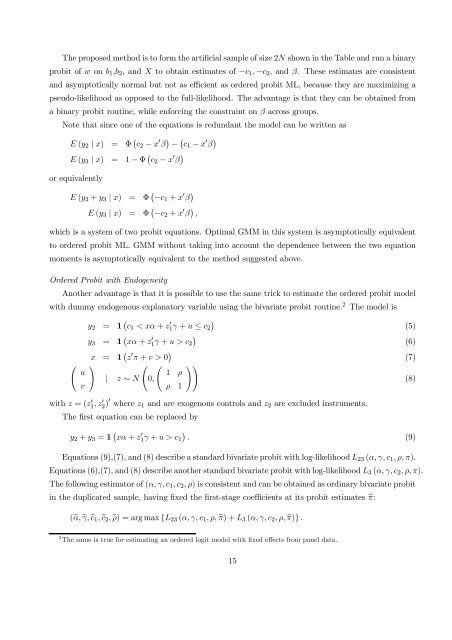
The proposed method is to form the artificial sample of size 2N shown in the Table and run a binary
probit of w on b1,b2, andXto obtain estimates of −c1, −c2, and β. These estimates are consistent
and asymptotically normal but not as efficient as ordered probit ML, because they are maximizing a
pseudo-likelihood as opposed to the full-likelihood. The advantage is that they can be obtained from
a binary probit routine, while enforcing the constraint on β across groups.
Note that since one of the equations is redundant the model can be written as
E (y2 | x) = Φ ¡ c2 − x 0 β ¢ − ¡ c1 − x 0 β ¢
E (y3 | x) = 1−Φ ¡ c2 − x 0 β ¢
or equivalently
E (y2 + y3 | x) = Φ ¡ −c1 + x 0 β ¢
E (y3 | x) = Φ ¡ −c2 + x 0 β ¢ ,
which is a system of two probit equations. Optimal GMM in this system is asymptotically equivalent
to ordered probit ML. GMM without taking into account the dependence between the two equation
moments is asymptotically equivalent to the method suggested above.
Ordered Probit with Endogeneity
Another advantage is that it is possible to use the same trick to estimate the ordered probit model
with dummy endogenous explanatory variable using the bivariate probit routine. 2 The model is
y2 = 1 ¡ c1 c2
(6)
x = 1 ¡ z 0 π + v>0 ¢
(7)
à !
à à !!
u
1 ρ
| z ∼ N 0,
(8)
v
ρ 1
with z =(z 0 1 ,z0 2 )0 where z1 and are exogenous controls and z2 are excluded instruments.
The first equation can be replaced by
y2 + y3 = 1 ¡ xα + z 0 ¢
1γ + u>c1 . (9)
Equations (9),(7), and (8) describe a standard bivariate probit with log-likelihood L23 (α, γ,c1, ρ, π).
Equations (6),(7), and (8) describe another standard bivariate probit with log-likelihood L3 (α, γ,c2, ρ, π).
The following estimator of (α, γ,c1,c2, ρ) is consistent and can be obtained as ordinary bivariate probit
in the duplicated sample, having fixed the first-stage coefficients at its probit estimates bπ:
(bα, bγ, bc1, bc2, bρ) = arg max {L23 (α, γ,c1, ρ, bπ)+L3 (α, γ,c2, ρ, bπ)} .
2 The same is true for estimating an ordered logit model with fixed effects from panel data.
15