Binary Models with Endogenous Explanatory Variables 1 ... - Cemfi

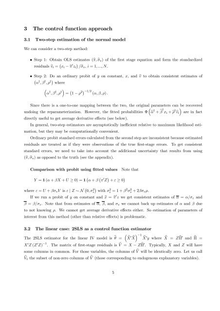
3 The control function approach
3.1 Two-step estimation of the normal model
We can consider a two-step method:
• Step 1: Obtain OLS estimates (bπ, bσv) of the first stage equation and form the standardized
residuals bvi = ¡ xi − bπ 0 ¢
zi /bσv, i =1, ..., N.
• Step 2: Do an ordinary probit of y on constant, x, andbv to obtain consistent estimates of
¡ α † , β † , ρ † ¢ where
³
α † , β † , ρ †´
= ¡ 1 − ρ 2¢ −1/2 (α, β, ρ) .
Since there is a one-to-one mapping between the two, the original
³
parameters can be recovered
undoing the reparameterization. However, the fitted probabilities Φ bα † + b β † xi + bρ † ´
bvi are in fact
directly useful to get average derivative effects (see below).
In general, two-step estimators are asymptotically inefficient relative to maximum likelihood estimation,
but they may be computationally convenient.
Ordinary probit standard errors calculated from the second step are inconsistent because estimated
residuals are treated as if they were observations of the true first-stage errors. To get consistent
standard errors, we need to take into account the additional uncertainty that results from using
(bπ, bσv) as opposed to the truth (see the appendix).
Comparison with probit using fitted values Note that
Y = 1 (α + βX + U ≥ 0) = 1 ¡ α + β ¡ π 0 Z ¢ + ε ≥ 0 ¢
where ε = U + βσvV is ε | Z ∼ N ¡ 0, σ2 ¢
ε with σ2 ε =1+β 2 σ2 v +2βσvρ.
If we run a probit of y on constant and bx = bπ 0 z we get consistent estimates of α = α/σε and
β = β/σε. Note that from estimates of α, β, andσvwe cannot back up estimates of α and β due
to not knowing ρ. We cannot get average derivative effects either. So estimation of parameters of
interest from this method (other than relative effects) is problematic.
3.2 The linear case: 2SLS as a control function estimator
The 2SLS estimator for the linear IV model is bθ =
³
bX 0 ´ −1
bX bX 0y where bX = Z bΠ 0 and bΠ =
X0Z (Z0Z) −1 . The matrix of first-stage residuals is bV = X − Z bΠ 0 . Typically, X and Z will have
some columns in common. For those variables, the columns of bV will be identically zero. Let us call
bV1 the subset of non-zero columns of bV (those corresponding to endogenous explanatory variables).
5