Binary Models with Endogenous Explanatory Variables 1 ... - Cemfi

More documents

Recommendations

Info

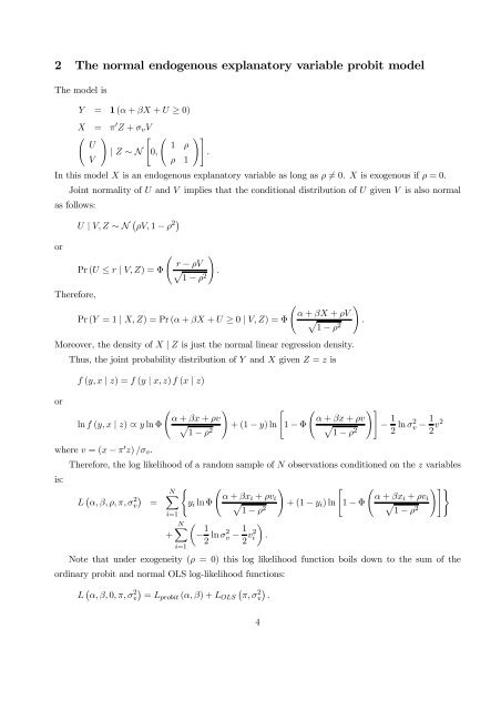
2 The normal endogenous explanatory variable probit model The model is Y = 1 (α + βX + U ≥ 0) X = π 0 Z + σvV Ã ! " Ã !# U 1 ρ | Z ∼ N 0, . V ρ 1 In this model X is an endogenous explanatory variable as long as ρ 6= 0. X is exogenous if ρ =0. Joint normality of U and V implies that the conditional distribution of U given V is also normal as follows: U | V,Z ∼ N ¡ ρV,1 − ρ 2¢ or Therefore, Ã ! Pr (U ≤ r | V,Z) =Φ r − ρV p 1 − ρ2 . Pr (Y =1| X, Z) =Pr(α + βX + U ≥ 0 | V,Z) =Φ Ã ! α + βX + ρV p . 1 − ρ2 Moreover, the density of X | Z is just the normal linear regression density. Thus, the joint probability distribution of Y and X given Z = z is or f (y, x | z) =f (y | x, z) f (x | z) Ã ! " Ã ln f (y, x | z) ∝ y ln Φ α + βx + ρv p 1 − ρ2 +(1−y)ln 1 − Φ !# α + βx + ρv p − 1 − ρ2 1 2 ln σ2v − 1 2 v2 where v =(x− π0z) /σv. Therefore, the log likelihood of a random sample of N observations conditioned on the z variables is: L ¡ α, β, ρ, π, σ 2 ¢ NX ( Ã ! " Ã !#) α + βxi + ρvi α + βxi + ρvi v = yi ln Φ p +(1−yi)ln 1 − Φ p 1 − ρ2 1 − ρ2 i=1 + NX i=1 µ − 1 2 ln σ2v − 1 2 v2 i . Note that under exogeneity (ρ =0) this log likelihood function boils down to the sum of the ordinary probit and normal OLS log-likelihood functions: L ¡ α, β, 0, π, σ 2¢ ¡ ¢ 2 v = Lprobit (α, β)+LOLS π, σv . 4
3 The control function approach 3.1 Two-step estimation of the normal model We can consider a two-step method: • Step 1: Obtain OLS estimates (bπ, bσv) of the first stage equation and form the standardized residuals bvi = ¡ xi − bπ 0 ¢ zi /bσv, i =1, ..., N. • Step 2: Do an ordinary probit of y on constant, x, andbv to obtain consistent estimates of ¡ α † , β † , ρ † ¢ where ³ α † , β † , ρ †´ = ¡ 1 − ρ 2¢ −1/2 (α, β, ρ) . Since there is a one-to-one mapping between the two, the original ³ parameters can be recovered undoing the reparameterization. However, the fitted probabilities Φ bα † + b β † xi + bρ † ´ bvi are in fact directly useful to get average derivative effects (see below). In general, two-step estimators are asymptotically inefficient relative to maximum likelihood estimation, but they may be computationally convenient. Ordinary probit standard errors calculated from the second step are inconsistent because estimated residuals are treated as if they were observations of the true first-stage errors. To get consistent standard errors, we need to take into account the additional uncertainty that results from using (bπ, bσv) as opposed to the truth (see the appendix). Comparison <strong>with</strong> probit using fitted values Note that Y = 1 (α + βX + U ≥ 0) = 1 ¡ α + β ¡ π 0 Z ¢ + ε ≥ 0 ¢ where ε = U + βσvV is ε | Z ∼ N ¡ 0, σ2 ¢ ε <strong>with</strong> σ2 ε =1+β 2 σ2 v +2βσvρ. If we run a probit of y on constant and bx = bπ 0 z we get consistent estimates of α = α/σε and β = β/σε. Note that from estimates of α, β, andσvwe cannot back up estimates of α and β due to not knowing ρ. We cannot get average derivative effects either. So estimation of parameters of interest from this method (other than relative effects) is problematic. 3.2 The linear case: 2SLS as a control function estimator The 2SLS estimator for the linear IV model is bθ = ³ bX 0 ´ −1 bX bX 0y where bX = Z bΠ 0 and bΠ = X0Z (Z0Z) −1 . The matrix of first-stage residuals is bV = X − Z bΠ 0 . Typically, X and Z will have some columns in common. For those variables, the columns of bV will be identically zero. Let us call bV1 the subset of non-zero columns of bV (those corresponding to endogenous explanatory variables). 5
Page 1 and 2: 1 Introduction Binary Models with E
Page 3: In these circumstances it is natura
Page 7 and 8: 3.3.1 Constructing policy parameter
Page 9 and 10: Local average treatment effects (LA
Page 11 and 12: A 2SLS as a control function estima
Page 13 and 14: Thus, √ ³ ´ N bθ d→ − θ0
Page 15: The proposed method is to form the

Binary Models with Endogenous Explanatory Variables 1 ... - Cemfi

Create successful ePaper yourself

Delete template?

Save as template?