Does Alma Mater matter? Evidence from Italy*

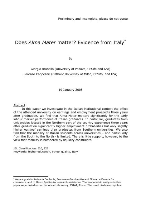
Preliminary and incomplete, please do not quote 

Does Alma Mater matter? Evidence from Italy * 

By 

Giorgio Brunello (University of Padova, CESifo and IZA) 

Lorenzo Cappellari (Catholic University of Milan, CESifo, and IZA) 

19 January 2005 

Abstract 

In this paper we investigate in the Italian institutional context the effect 

of the attended university on earnings and employment prospects three years 

after graduation. We find that Alma Mater matters significantly for the early 

labour market performance of Italian graduates. In particular, graduates from 

universities located in the Northern part of the country experience three years 

after graduation significantly higher employment probabilities but only slightly 

higher nominal earnings than graduates from Southern universities. We also 

find that the mobility of Italian students across universities – and particularly 

from the South to the North - is limited. There is little support, however, to the 

view that mobility is hampered by liquidity constraints. 

JEL Classification: I20, I22 

Keywords: higher education, school quality, Italy 

* We are grateful to Maria De Paola, Francesca Gambarotto and Eliana La Ferrara for 

comments, and to Marco Spaltro for research assistance. The econometric analysis in this 

paper was carried out at the Adele Laboratory, ISTAT, Rome. The usual disclaimer applies.

Introduction 

Does the attended college affect the earnings and employment prospects 

of graduates? This question is particularly important for the households 

sending their offspring to college and paying part of the cost, and for the 

government, which in a number of countries runs most universities and needs 

to know whether and why some institutions may be delivering better outcomes 

than others. 

Spurred by the interest on the quality of education, a recent literature 

has investigated the labour market effects of college quality, mainly but not 

exclusively in the US. Black and Smith, 2003, and Brand and Halaby, 2003, 

review the key contributions. The main focus in this literature has been so far 

on comparing elite versus non – elite colleges, and the degree of selectivity 

has been measured either with the average SAT score of the incoming 

freshmen – in the US – or with the average A-level score of the intake of 

students – in the UK (see Chevalier and Gonlon, 2003). The basic finding of 

this literature is that college quality matters for labour market outcomes. 

In this paper we investigate in the Italian institutional context the effect 

of the attended university on earnings and employment prospects three years 

after graduation. Since we cannot measure unambiguously selectivity, we 

focus instead on the location of the college, on the public/private divide and on 

observable measures of college quality. We find that Alma Mater matters 

significantly for the early labour market performance of Italian graduates. In 

particular, graduates from universities located in the more developed Northern 

part of the country experience three years after graduation significantly higher 

employment probabilities but only slightly higher nominal earnings than 

graduates from Southern universities. 

We also find that the mobility of Italian students across universities – 

and particularly from the under-developed South to the more developed North 

- is limited. There is little support, however, to the view that mobility is 

hampered by liquidity constraints. Alternative explanations include regional 

price differentials, which reduce the earnings gap between the North and the 

1

South – and can even turn the gap into an advantage, and the possibility that 

uncovered differences are temporary. The finding that the expected returns to 

college are not significantly higher for the graduates of Northern universities 

combines with the higher cost of living, opportunity costs and tuition fees in 

the North to explain why so many Southern students still prefer to enrol in the 

South. 

We also find that going to a private university matters especially for the 

probability of finding a job, but not always in a positive way. Heterogeneity in 

early labour market returns spread from public to private universities. When 

the attended private college yields negative employment and earnings gains, 

the question arises why households should enrol their offspring in such 

institutions at a higher tuition fees than in public universities. The natural 

explanation is that these losses are temporary, and turn into gains as labour 

market experience increases. Religious and cultural reasons, access to 

networks and leisure are additional and not necessarily mutually exclusive 

explanations. 

Available indicators of college quality explain some but not all the 

difference between private and public tertiary education. There is evidence that 

the pupil – teacher ratio, the size of the university – in terms of the number of 

enrolled students - and the proportion of female teachers affect in a 

statistically significant way either wages or employment or both. The location 

of the college also matters, as universities located in the South usually deliver 

inferior outcomes. 

The policy implications clearly depend on whether the effects of 

measured college quality three years after graduation persist over time. While 

limited mobility from lower to higher performing universities suggests that 

some of these effects are temporary, better data than those available are 

required to answer this key question. In particular, it would be critical to re- 

interview graduates at regular times during their career, as in the UK Graduate 

Cohort Study, which repeats interviews three, six and eleven years since 

graduation. 

2

Assuming that the uncovered effects are at least in part permanent, they 

suggest that policies favouring the diffusion of universities in the Italian 

territory need not be farsighted, as employment probabilities are significantly 

higher with larger – and older - institutions, possibly because of their 

entrenched reputation in the labour market. Policies promoting equal 

opportunity and a higher percentage of female professors have ambiguous 

labour market effects, negative on male graduates and positive on female 

graduates. Finally, and conditional on measured quality and on local labour 

market effects, Southern universities perform less satisfactorily than the 

universities in the rest of the country. Understanding why this is the case is an 

important area of policy evaluation. 

The paper is organized as follows. Section 1 provides some institutional 

background; Section 2 discusses the empirical approach; Section 3 introduces 

the data and Section 4 presents the results. Conclusions follow. 

1. Institutional background 

By international standards, Italy has 10 graduates out of 100 individuals 

aged 25 to 64, significantly lower than the OECD average of 15. Relatively low 

attainment is matched by a relatively low rate of return, 6.5 percent per year 

of college education, compared to 11.8 percent in the main developed 

economies (see OECD, 2003). Assuming a downward sloping demand for 

college education and an upward sloping supply, the combination of low 

attainment and low returns suggests that the relative demand for college 

graduates in Italy is relatively low by international standards 1 . 

Reasons for relative low demand could be that the Italian industrial 

structure is biased against higher education, or that the perceived quality of 

tertiary education is low, or both. According to the OECD, Italy spends less 

than the major developed economies for tertiary education. In the year 2000, 

the average expenditure per student was 8065 US dollars, compared to 8373 

dollars in France, 10898 dollars in Germany, 9657 dollars in the UK and 20358 

dollars in the US. Low expenditure is partly due to the fact that average pay in 

1 See Brunello, Comi and Lucifora, 1999, and Checchi and Jappelli, 2004, and Checchi, 2002. 

3

universities is low and partly to a higher than average students to teacher ratio 

(22.4 compared to the OECD average of 16.5 2 ). Moreover, Italy has a 

relatively low share of private universities, which enrol only 6.4 percent of 

college students, compared to 12 in the OECD average. 

Only 10.9 percent of the budget comes from tuition fees. See Perotti, 

2002, for a very good discussion of the funding of Italian universities. 

2. Empirical strategy 

The recent literature on the estimation of college quality (wage-) effects 

highlights a few issues inherent to such exercise. Specifically, Black and Smith 

(2003) discuss the pitfalls that a standard log-wage regression could lead to, 

and how matching estimators can solve/mitigate those issues. First, there is 

the issue of selection on unobservables, omitted variable bias in the language 

of linear regression: as long as factors that influence both treatment receipt (in 

their case college quality) and the outcome (earnings) are omitted from the 

estimating model, resulting effects are biased and inconsistent. Second, there 

is the issue of common support, multicollinearity in the language of linear 

regression: in order for the effect to be identified the variability of the 

treatment over the sample must not be already captured by other covariates in 

the model, which is achieved when there are cells defined by the intersection 

of the covariates in which both treated and non-treated individuals are 

observed. Black and Smith stress an important implication of this property: the 

effect estimated by a linear regression is identified non-parametrically only in 

the common support, while outside the common support it is a parametric 

projection of the effect estimated using observations in common support. 

Thirdly, and finally, they point to the issue of linear conditioning on 

observables, functional form misspecification in the language of linear 

regression: even if all the relevant personal attributes are controlled for, an 

omitted variable bias could emerge if they enter the estimating equation with 

an inappropriate functional form. The Black and Smith approach is to resort to 

2 Notice that Italy has a very low ratio in primary and secondary education, as discussed in detail by Brunello and 

Checchi, 2004. Perotti, 2002, contains an interesting comparison between the Italian and the British higher education 

systems. 

4

a (propensity score) matching estimator. As explained in their paper, such an 

approach: a) assumes that there is no selection on unobservables problem; b) 

‘…does not solve the support problem… (page 5)’; and c) solves the linear 

conditioning issue, since rather than assuming that the expected value of the 

outcome conditional on the observables is a linear function of the observables, 

makes a fully non-parametric comparison of mean outcomes between treated 

and non-treated individuals in the common support. 

In this paper we take a different estimating approach, which we illustrate 

by focussing on wages as the outcome of interest (we also study employment 

probabilities and we detail later our methodology in that case). Let 

wi=αw+ΣfΣcd cf iθ cf +xi’γw+ui (1) 

be the log-monthly wage for individual i (i=1…N), a linear function of the 

college-faculty cluster from which she graduated (d cf i) and observable 

attributes (xi). The vector of observables includes controls for gender, region of 

employment, labour market experience parental background in terms of 

occupation and education, the final graduation mark, the type of high school 

attended (whether generalist or technical/professional) and the marks reported 

in the high school graduation exam. Given the inclusion of detailed parental 

background, these latter variable are likely to proxy the impact of ability. Most 

importantly, we allow for interactions between parental education and 

occupations, on the one hand, and marks and school types, on the other. 

Therefore, we allow all regressors related to personal attributes to enter the 

model non-linearly, which might result in an attenuation of the risks of 

misspecifying functional form. As for the first problem discussed in Black and 

Smith (2003), we assume, as they do, selection on observables, and specify a 

rather extended list of observables. Finally, we can not identify effects on 

college faculty dummies for which there is no common support. 

Regression (1) serves as the first step in our procedure and allows us to 

predict log-monthly earnings by college/faculty clusters. In the second step, 

we take an approach a-là- Card and Krueger (1991) and analyse the 

5

determinants of college/faculty wage effects. Specifically, let q cf be the 

estimate of θ cf from (1). Let q be the vector stacking these estimates: they 

are the mean wages by college-faculty clusters. In the second step of our 

procedure, we estimate the effect of several dimension of college quality by 

regressing estimated wage effects on college quality measures derived from 

published sources or other measures of college heterogeneity, plus college and 

faculty fixed effects. We employ a Weighted Least Squares, using weights 

proportional to the (inverse) of var(q) to account for the fact that our 

dependent variables are estimates from the first stage. 

As we said above, we also analyse the impact of Alma Mater on 

employment probabilities. In that case, equation (1) is substituted by a probit 

equation, the dependent variable scoring one for the employed and zero 

otherwise. 3 From such a probit equation we can estimate the employment 

probability (and its variance) for each college/faculty cluster, which we then 

employ as dependent variable (and weight) in the second step regression. 

3. The Data 

The National Statistical Office (ISTAT) carries out on a regular basis a 

statistical survey – the “Indagine statistica sull’inserimento professionale dei 

laureati” - on the transition from college to work of a representative sample of 

Italian graduates. The last available wave interviews individuals who graduated 

in 1998 three years after completion of the degree, in 2001. The survey covers 

school curriculum, labour market experience in the three years after 

graduation, job search activities, household and individual information. We 

match these data with the information on college quality disaggregated by field 

of study and provided by ISTAT for the academic year 1996-7 4 . 

We focus our analysis on the effects on the college on the probability of 

being employed three years after graduation and on net monthly earnings in 

the job held at the time of the interview. Employment in the survey includes all 

3 

In this case, the conditioning set excludes labour market experience, while regions of work are substituted by regions 

of birth. 

4 

ISTAT, Lo stato dell’università, several issues. Since the publicly available micro-data do not include the university 

the interviewed individual graduated from, we carried out the matching at the ADELE ISTAT laboratory in Rome. 

6

paid jobs, including apprenticeship contracts 5 . About 4 percent of the currently 

employed are on a training contract – which includes post-graduate education. 

This percentage raises to close to 44 percent among those not currently 

working. Monthly earnings in 2001 are in euros and net of taxes and social 

security contributions 6 . Average earnings in the sample are 1140,1 euros per 

month, with a standard deviation of 422.8, and range from a minimum of 

103,2 € to a maximum of 4389,8 €. On the other hand, the average probability 

of being employed three years after graduation is 0.664, with a standard 

deviation of 0.472. 

Table 1 shows average pay and employment probability by gender, type 

of college – public or private – and area where the college is located. On 

average, male graduates earn about 25 percent more than females, and are 

more likely to have a paid job three years after graduation. Having graduated 

from a private college yields a close to 10 percent wage premium, and a close 

to 20 percent premium in the probability of employment. Finally, graduation 

from a college located in the Northwest yields a 20 percent wage premium and 

a close to 50 percent higher employment probability than having graduated in 

a Southern college. The regional wage premium falls considerably from 20 to 

8.3 if we compare individuals who graduated from a college in the Northwest 

and work in the same area with individuals who graduated in the South but 

work in the Northwest. 

Table 1. Average earnings and employment probability by gender, type of 

college and college area 

Average 

Average 

monthly earnings employment probability 

Male 1249,6 0,716 

Female 1040,0 0,622 

Private college 1239,5 0,793 

Public college 1132,3 0,655 

College located in Northwest Italy 1218,2 0,773 

5 The relevant question is: “Are you now – at the time of the survey – on a paid job? “ Only a very small minority of 

those not currently employed were employed in the week before the interview. Since we do not have information on 

wages, we drop these individuals from the sample. 

6 Earnings in the publicly available data are provided in ranges rather than as a continuous variable. All our 

computations based on continuous variables were carried out at the ADELE ISTAT laboratory in Rome. 

7

College located in Northeast Italy 1124,7 0,733 

College located in Central Italy 1121,0 0,631 

College located in Southern Italy 1054,6 0,513 

Needless to say, these averages are affected by individual 

characteristics, the college and the field of study. Table 2 reports average 

earnings and employment probabilities in 16 fields of study, which correspond 

to different faculties. 

Average earnings are highest for graduates in Medicine, who face on the 

other hand the lowest employment probability, and lowest for graduates in 

Foreign Languages. Figure 1 and Figure 2 show that both earnings and 

employment probabilities vary substantially within each field of study by 

college. The within-field of study variation in earnings – measured by the 

coefficient of variation - is highest for the graduates in Medicine, Sociology and 

Statistics. In the former field, a graduate from Verona and Padova earn per 

month close to 100 percent more than a graduate from Pisa and L’Aquila. 

Table 2. Average earnings and employment probability by field of study 

Average monthly earnings Average 

Employment probability 

Agricultural studies (AG) 1127,2 0,636 

Architecture (AR) 1077,3 0,696 

Economics and Business (EC) 1163,9 0,752 

Pharmacy (PH) 1174,1 0,788 

Law (LA) 962,9 0,479 

Engineering (EN) 1298,8 0,854 

Humanities (HU) 949,5 0,589 

Foreign languages (FO) 910,6 0,632 

Medicine (ME) 1531,7 0,201 

Veterinary (VE) 1118,3 0,605 

Psychology (PS) 966,4 0,686 

Teachers college (TE) 956,4 0,670 

Natural sciences (SC) 1073,2 0,607 

Political Science (PO) 1104,8 0,735 

Statistics (ST) 1191,2 0,740 

Sociology (SO) 1048,8 0,582 

8

In the latter field, a graduate from Florence earns on average 84 percent 

more per month than a graduate from Messina. Moreover, the average 

monthly earnings of a graduate in Economics from Bocconi University, a 

private institution, are about 60 percent higher than the earnings of a graduate 

in the same field from the University of Benevento, at the bottom of the list. 

Turning to employment probabilities, it is always the case that these are 

lowest for graduates of Southern colleges, independently of whether they look 

for a job in the North or in the South of the country. For example, a graduate 

in Engineering from the University of Trieste has a probability of employment 

after three years close to 1, compared to less than 0.6 for a graduate from 

Potenza, in the deep South. 

Figure 1. Within field variation in average earnings 

average log earnings 

2500 

2000 

1500 

1000 

500 

TOPOL 

TO 

TO 

TO 

TOPOL 

VC 

NO 

TO 

TO TO 

AL 

TO 

TO 

TO TO 

AL 

TO 

AL 

GE 

GE 

GE 

GE 

CO 

MIBOC 

MIPOL 

MICAT 

GE 

MICAT MISTA 

MISTA 

MISTA 

MISTA 

GE 

MICAT 

MIPOL 

MISTA 

MISTA 

MICAT 

MICAT 

MICAT MISTAMISTA MISTA 

BSCAT 

MICAT GE 

GE 

GE 

GE 

GE 

BSCAT BSCAT 

PV 

PV 

BS 

BG BS 

MIULM 

PC 

PV MIBIC 

ROCAT 

PV PV 

PV 

PC 

PV BS 

MIULM BG 

PV 

PV 

PD 

TN VE 

VR 

VR 

PD 

TN 

VE 

PD 

TN VR VR VE 

PD 

TN VR 

VE PD 

PD 

PD 

TN 

PD 

PD 

PD 

FE 

TS 

MO 

BO 

MO FE 

UD 

UD TS TS FE 

PD 

PR UD 

PR BO 

PR PR 

PR 

BO 

MO BO TS 

UD 

BO 

PR 

BO 

UR MO 

BO 

FE FE 

PR PR MO BO TS FE 

BO 

UR 

FE 

MO TS BO PR 

FO 

UR 

UR 

UD BO 

BO 

TS UR 

UR 

UR 

SI 

FI 

PG AN FI 

PG 

PI 

AN 

PI FI 

PG PI 

PI 

MC AN PI SI FI PG 

SI 

FI 

FI FI 

AN 

FI 

SI 

MC PI 

PI SI SI 

FI 

MC 

PI FI PI PI 

PI 

UR 

PG PG FI 

MC SI 

MC 

PG 

ROSAP 

PG 

ROSAP ROSAP 

VT 

ROSAP 

PG 

ROSAP PG 

ROSAP 

ROSAP 

ROSAP 

ROSAP PG 

ROSAP 

ROSAP 

ROTOR 

ROTOR 

ROTOR 

ROLUM 

ROTRE ROLUI ROLUI 

ROTOR 

CAS ROSAP 

ROLUI 

NAFED ROTRE 

CAS 

ROTRE 

CASROTRE 

BV 

ROTOR 

ROTOR 

NAFED 

SA 

CH 

NAFED 

AQ 

NAFED NAFED 

AQ 

BA 

CH BA 

PS 

NAPAR 

SA 

NAFED 

BA 

FG 

PS TE 

AQ NASEC NAFEDNAFED SA 

NASEC SA 

NAORS 

AQ AQNAFED 

CB NAORI CH 

CB 

NAORS 

NAFED NAORI 

NAORI CB 

SA BA 

NAFED SA 

TE 

BA 

SA 

NAORS 

SA 

PS 

BA 

BA 

BAPOL 

CS 

PT 

LE 

BA 

PA 

RC 

LE 

PT 

LE 

BA 

PA 

PT 

CS 

CS 

BA 

PA 

CZ LE 

CZ 

LE 

CS 

LE 

CS 

PA 

PA 

CA CT 

MS 

CT 

CA PA 

SS MS 

CT 

MS MS SS 

SS 

CA 

PA CT 

MS 

SS 

SS 

CT 

CT 

PA 

MS 

MS SS 

MS 

CT 

CT PA 

PA CA CT 

MS PA 

CT 

CA 

PA 

PA MS CA 

MS 

CT 

CA 

SS 

SS 

SS CA 

SS 

FG 

NAFED 

AG AR EC PH LA EN HU FO ME VE PS TE SC PO ST SO 

field 

Note: see the legend in the Appendix 

9 

VR 

PD 

BO 

NASEC 

TO BS FI 

MS TS 

NAFED 

MISTA 

TN 

UR 

ROSAP 

SA 

NAFED

average employment probability 

Figure 2. Within field of study variation in employment 

1 

.8 

.6 

.4 

.2 

0 

FE 

MISTA 

BO 

MIPOL VE 

PD 

PC 

TO TOPOL FI 

ROSAP 

FI GE 

PI 

CT 

UD PA 

NAFED 

VR BA PS 

NAFED 

RC 

PG PT 

VT 

PA 

NO 

TO 

VC 

TOPOL 

TO 

TO 

GE AL 

TO 

TO 

TO 

TO 

TO 

TO 

TO AL 

TO AL 

GE 

SI 

TS 

CO MISTA MIPOL UD AN PV 

MICAT MO PD 

ROLUI 

ROTOR BSCAT MICAT 

PC 

ROSAP BAPOL 

PI 

MIBOC BS PV PD MO BO 

ROSAP 

TN 

FI GE MICAT VR 

BS PV 

BG UD 

MIULM 

VR PR TN 

PG 

CT 

PV 

PG 

PR 

ROTRE MC FE NAFED MS AQ BG 

MICAT UD 

ROTOR VE 

FE 

PI SI 

LE 

BV PR 

FI 

MO FI 

SS 

BO 

PD TN 

CT PI 

PG 

BO UR 

ROSAP 

PD 

CASNAFED 

BA 

MISTA PV 

UR 

VR 

MISTA 

PD 

TS 

PA TS CS 

BO UR 

SA PA 

TS PV TS PR BO FO 

PG AN 

BA 

PG 

CH 

ROTRE 

CAS 

BO VE FI ROSAP SS 

NASEC 

NAPAR SA ROLUI MC 

NAFED CT SS 

PA PR 

PI 

LE 

CS 

MS MICAT FE 

GE VE MISTA 

PD PR 

FE PI SI 

MS 

CB 

MS 

ROTRE 

MC PS 

CT 

SS 

PS 

MISTA MO UR ROSAP SA NAORI PI 

FG 

CS 

BS PT 

UR CH CA 

ROSAP 

NASEC CA 

MC 

TN PA FI SS PA PG 

GE ROTOR 

PG 

BA PA 

SI CS CT 

MS 

GE 

PA 

ROTOR BO CA CZ SS 

PI NAORI BA 

NAORS NAFED 

ROSAP 

BA 

MIBIC MC MS SA CH 

ROTOR SI 

NAFED 

NAFED 

MS CT 

FG 

GE AQ 

LE MISTA 

SA TE 

CA PT AN TS 

PI 

NAORS BS FI 

LE BO PD PV 

PA 

SS 

CB 

NAFED ROSAP VR 

NAFED MO 

MS 

PG BA 

PR 

FE 

NASEC CT 

ROCAT CA 

MIULM 

MICAT MISTA MISTA 

GE VR AQ UD 

BSCAT 

BO PD TS ROSAP 

BO PD 

PR BSCAT GE PV PI FI BO 

PG UR MICAT UR 

TN 

PD 

MO 

FI FE SI FI 

MISTA PG ROSAP 

ROLUI 

AQ PR 

ROTOR PV BA CT 

MC GE SA 

BA CB SS 

CAS BO PD ROLUM 

CT TE 

FI BA 

UR ROSAP NAFED CZ 

ROTRE 

AQ SI 

PA 

PA SS 

PI 

TS LE 

NAORS CA 

SA 

NAORI 

NAFED 

NAFED LE CS PA 

CT MS MS 

SS 

AN SA CA 

MS 

CA 

MS 

TN 

UR 

ROSAP 

SA 

NAFED 

AG AR EC PH LA EN HU FO ME VE PS 

field 

TE SC PO ST SO 


Next, we compare the average earnings and employment probabilities of 

graduates of public and private colleges – by restricting attention to 

economics, which include a few private universities. Figures 3 and 4 show that 

private colleges do better on average than public colleges, both for earnings 

and for employment. Some private universities, however, perform worse in 

terms of earnings and at least as well in terms of employment as top public 

institutions. 

10

Figure 3. Average monthly earnings in public and private colleges - Economics 

average monthly earnings 

1600 

1400 

1200 

1000 

800 

PV 

BG 

TO 

BS 

VE 

UD TN 

VR 

GE 

NO 

TS 

ROTOR 

PG 

ROSAP ROTRE 

PR SS 

NAPAR MC AN 

BA 

MO BO 

PI SI 

NAFED 

FG 

PA FI 

UR PS 

LE 

MS SA 

NASEC CT 

CS 

CAS 

CB 

BV 

0 1 

private university 

monthly earnings of graduates in economics 


Figure 4. Average employment probability in public and private colleges 

average monthly earnings 

1 

.8 

.6 

.4 

.2 

0 

NO 

BS PV 

ROTRE MC 

UD BG PR VR TN 

ROTOR TO VE 

MO 

GE 

BV PI SI 

FI 

ROSAP CAS 

TS 

BO UR 

PG AN 

BA 

NAPAR SA 

NAFED CT 

PA 

SS 

LE 

MS 

CB 

CS PS 

FG 

NASEC 

0 1 

private university 

employment probability of graduates in economics 


For instance, the graduates of Roma Luiss, a private college, earn on 

average about the same as the graduates of Roma Tre and Roma La Sapienza, 

but less than the graduates of Rome Tor Vergata, a public institution located in 

the same city. On the other hand, the graduates of Bocconi University earn on 

average more than the graduates of other Milanese universities, both public 

and private. 

11 

MICAT CO 

ROLUI PC 

MIBOC 

CO 

MIBOC 

MICAT 

ROLUI 

PC

Both private and public colleges generate heterogeneous outcomes in the 

labour market. Part of this heterogeneity could fade away over time, as 

graduates settle in their jobs, but part could depend on measurable differences 

in inputs and outputs. Table 3 illustrates some of these differences, separately 

for public and private colleges. 

Table 3. Differences in inputs and outputs, by type of college 

12 

Public college Private college 

Year when the faculty was established 1932 1958 

Student / teacher ratio 41.69 25.78 

Percentage of students not completing their degree in the 

requested time 

38.61 38.42 

Number of students 4605 3698 

Percentage of graduates over enrolled students 7.54 11.76 

Note: the year of establishment is coded as 1800 if the college was established in 1800 or before. 

The table shows that private universities tend to be younger, smaller, 

and have a significantly lower ratio of students to teachers. While the average 

age of professors is about the same, the percentage of female professors is 

slightly lower, and the percentage of graduates over enrolled students 

significantly higher. The Data Appendix shows how these indicators vary across 

colleges and fields of study. 

The list of indicators in Table 3 cannot be considered as exhaustive. An 

indicator that is missing in our data is the average peer effect. This is an 

important measure if we believe, as Epple and Romano, 1998, that school 

quality critically depends on the average quality of enrolled students. Another 

missing indicator is a measure of network effects, which might play an 

important role if private colleges provide access to better networks, and if 

these networks are important in the search of a good job, as suggested for 

Italy by Pellizzari, 2003. Finally, we miss information of teacher quality. The 

recent literature on school quality (see Hanushek, 2002, for a survey), clearly 

emphasizes this variable as key to explain school performance.

4. Results 

In the first step regressions (REPORT IN THE APPENDIX), we fit 

individual earnings and employment probabilities separately by gender on 411 

college by field of study dummies, individual experience, experience squared, 

number of siblings, cohort of birth dummies, type of job (whether the current 

job is part time or full time), dummies for additional years in college after the 

required years, dummies for the region of current residence, individual 

graduation marks – relative to the highest attainable mark – type of school 

before college, graduating marks in upper secondary education, family 

background – measured by the education and occupation of both parents when 

the individual was 14 years of age – and interactions between education before 

college and family background. The maintained hypothesis is that performance 

at school before college, family background and their interactions fully capture 

unobserved individual ability, which affects earnings as well as selection into 

employment. 

4.1 College effects on wages and employment 

We interpret the estimated coefficients of the 411 dummies as the net 

impact of college and field of study on individual earnings and employment 

three years after graduation. Under our maintained assumption, these 

estimates are consistent. We distinguish the net from the gross impact, 

because the college and field of study can affect some of the controls, such as 

labour market experience, performance in college, type of job, region of 

residence and actual time to complete the degree. We also compute the gross 

impact of college and field by re-estimating the first step regressions after 

excluding such controls. To save space, we present some results based on the 

gross effect in the Appendix. 

The region of residence three years after graduation does not necessarily 

coincide with the region where the college was located, as individuals migrate 

to the areas of the country where they can locate better matches. Table 4 

illustrates the mobility flows across the four macro areas of the country. As 

13

expected, individuals completing a degree in the Centre or in the South are 

more likely than individuals in the North to relocate and work in another 

macro-area, typically the North West, where many college jobs are located. In 

spite of these mobility flows, the percentage of individuals who currently reside 

in the same area where they went to college is at least equal to three quarters 

of the population of graduates. 

Table 4. Mobility flows among the four macro areas of Italy 

Residence Residence Residence Residence 

North West North East Centre 

South 

College North West 93.52 3.47 1.65 1.36 

College North East 12.30 81.87 3.86 1.97 

College Centre 6.95 3.95 75.91 13.18 

College South 9.17 3.34 6.87 80.62 

Note: the numbers in the table are percentages, which add up to 100 by row. 

We disentangle the contributions of the field of study and the university 

to the wage and employment effects by regressing the estimated net effects 

on separate field of study and college dummies. In order to have sufficient 

observations for each university, we restrict our attention to the institutions 

with at least five faculties. The college dummies in these regressions measure 

the effect of each university on earnings and employment, conditional on the 

field of choice and on the individual effects controlled in the first stage. As 

shown in Figures 5 and 6, the variation of college effects is substantial, both 

for wages and for employment. 

14

Figure 5. College effects on earnings, by gender 

males 

425 

277 

FE 

CA 

SS 

MC 

MS 

MO 

CS 

PV 

PA 

TS 

PR 

NAFED 

SA 

PD 

ROTOR 

181 236 

females 

Wage effects 

SI 

ROSAP 

15 

LE 

BO 

UR 

BA 

TN 

FI 

MICAT 

CT 

MISTA 

Figure 6. College effects on employment probability, by gender 

males 

.7 MO TN 

PV TO 

.6 

.5 

.4 

CA 

MS 

CS 

CT NAFED 

LE 

PA 

ROSAP 

PI SI 

PG 

SA 

.2 .4 .6 .8 

females 

Employment effects 

BA 

ROTOR 

SS 

AQ 

PR 

UR 

MC 

GE 

FI 

BO 

TS 

FE 

PI 

PD 

PG 

GE 

MISTA 

AQ 

TO 

MICAT 

Consider first wages. The difference between the highest and the lowest 

college effect is higher than 25 percent for both genders. For instance, male

graduates from the University of Trieste, in the North-East, earn 53 percent 

more on their current job three years after college than graduates from 

Cosenza, in the South of the country. Female graduates from Torino, in the 

North West, earn about 29 percent more than graduates from Ferrara, in the 

North-East. There is also a significant difference in the earnings of graduates 

from the largest universities in Rome – La Sapienza and Tor Vergata – and the 

largest colleges in Milan – Statale and Cattolica. For instance, male graduates 

from La Sapienza earn three years after graduation 16 percent less than male 

graduates from Statale. 

If we use the mean wage effects for males and females to divide the 

diagram in four quadrants, we discover some interesting heterogeneity. While 

Northern colleges tend to perform better than Southern colleges, there are 

exceptions: Ferrara and Modena, for instance, do well for males but poorly for 

females. On the other hand, Lecce is located in the outward quadrant, above 

both means. On average, Northern wage effects are 6.7 and 3.4 percent 

higher that Southern wage effects for maels and females respectively. 

Turning to employment probabilities three years after college, the 

difference across universities is large, with graduates from Turin enjoying a 

probability higher than 70 percent and graduates from Messina experiencing 

probabilities lower than 50 percent, independently of the region of current 

residence. Compared to earnings, the difference in employment probabilities 

for the graduates of the large universities located in Rome and Milan is 

negligible for males but large for females. Furthermore, the segregation of 

Southern colleges in the lowest quadrant near the origin is much more marked 

than in the case of wages. On average, Northern employment effects are 25 

and 32 percent higher that Southern wage effects for maels and females 

respectively. 

Figures 7 and 8 plot wage and employment effects by gender. A natural 

reading here is that the points in the figures lie on different demand curves, 

which express the labour market trade-off between earnings and employment 

probabilities. 

16

Figure 7. Wage and employment effects, by college. Males 

males 

wage effects 

450 

400 

350 

300 

250 

MS 

PA 

CA 

SS 

NAFED LE 

CT 

MC 

AQ 

GE 

TS 

MISTA 

.4 .5 .6 .7 

employment effects 

Males 

FE 

SA 

PG 

UR 

CS 

17 

ROTOR 

BA 

PR 

PD PI 

BO SI 

FI 

ROSAP 

TN 

MICAT TO 

PV MO 

Figure 8. Wage and employment effects, by college. Females 

females 

wage effects 

240 

220 

200 

180 

CA 

MS 

CT 

PG 

PI 

SI 

ROSAP 

NAFED 

SA 

ROTOR 

PA 

CS 

TO 

AQ 

GE MISTA 

.2 .4 .6 .8 

employment effects 

Females 

LE 

BA 

TN 

UR 

MO 

MC 

SS 

PR 

FI 

BO 

TS 

FE 

PV 

PD 

MICAT 

Focusing on males, the wage and employment effects in Figure 7 are 

delimited by a demand curve close to the origin and connecting the Southern 

colleges of Messina, Palermo, Catania, Cagliari and Cosenza, and by an

outward demand curve connecting several universities of the North, Trento, 

Torino, Milano Catholic, Modena, Pavia and one in the Centre, Florence. A 

similar reading is possible for female graduates in Figure 8. If we rank 

universities on the basis of the demand curve they lie upon, the North-South 

divide emerges quite clearly. This divide is driven by employment probabilities 

rather than by wages. 

If students were perfectly mobile across universities, and the private 

costs of graduating from each institution were homogeneous across the 

country, we would expect these large differences in college – specific labour 

market returns to be washed away. Mobility of university students, however, is 

limited. Our survey provides information both on the region of residence before 

going to college and on the region where the college is located. As shown by 

Table 5, there is very little mobility across macro-regions, not only in the 

Northern and Central areas, where many high performing universities are 

located, but also in the South, where universities are among the worst 

performing in the sample. More in detail, students who resided in the South 

before college either remain there for college (73.5%) or move to the nearby 

Centre (18.8%): less than 8% move to the North 7 . 

Table 5. Mobility flows among the four macro areas of Italy, before college and 

during college 

College College College College 

North West North East Centre South 

Before College North West 90.78 7.39 1.52 0.30 

Before College North East 3.79 93.41 2.50 0.31 

Before College Centre 0.88 4.79 93.69 0.64 

Before College South 3.56 4.04 18.86 73.54 


These number cover, however, some interesting heterogeneity within 

macro-areas. In the South, for instance, the percentage of students remaining 

in their region to go to college is higher than 80 percent in Sicily and Sardinia 

and close to 40 percent in Calabria. 

7 The differences in performance across universities are net of local labour market effects, because we control for region 

of residence dummies in the first step when estimating net wages and employment effects. 

18

How do we explain the limited mobility flows between macro-areas? One 

natural possibility is that low mobility depends on family background and on 

liquidity constraints. According to this story, the internal rate of return of 

graduating from a Northern college is higher than in the South, but the higher 

costs prevent many Southerners from enrolling in the North. Studying in a 

university located in the North is likely to be expensive for a Southern student 

for a number of reasons. First, tuition is higher. Even though fees are not high 

by international standards, Northern colleges have used to a much larger 

extent than other universities in the country the opportunity to raise tuition in 

the second part of the 1990s above the centrally established ceiling (Law 

122/94). This and the endogenous selection of students to college have implied 

that average tuition in 1995 was about 50 percent higher in Northern than in 

Southern public universities – 511 € versus 326 € at current prices (see 

Silvestri et al, 1996). Second, both opportunity and living costs – including 

housing – are higher in the North. Third and last, income support provided by 

the national and local government is considered to be largely inadequate to 

eliminate liquidity constraints, as documented by Silvestri et al, 1996. [NON 

SAREBBE MALE AVERE QUALCHE DATO SUI COSTI DI VIVERE FUORI CASA 

ALL’UNIVERSITA] 

If liquidity constraints had played a significant role in hampering the 

mobility of students from the South to the North, we would expect to find that 

inter-regional mobility is much lower for students belonging to less educated 

and less wealthy households. Surprisingly enough, this is not the case. If we 

replicate Table 5 separately for individuals with “good” and “poor” family 

background at age 14 – good background being defined when the father was 

an entrepreneur, a manager, a high ranked director, a teacher or a high 

ranked white collar, and bad background when the father was in a low paying 

occupation – there is no difference worth noticing – see Table 6 below. The 

percentage of students in our dataset residing in the South who went to 

college in the South is 72.99 percent if from a good family background and 

74.12 percent if from a bad background. On the other hand, the percentage of 

students residing in the South before college who moved to the North for 

19

college is 8.22 among those with good background and 6.94 percent among 

those with bad background. These differences remain small even when we 

measure background with parental education 8 . 

Table 6. Mobility flows among the four macro areas of Italy, before college and 

during college. 

Good bakground 







Bad background 







We conclude that liquidity constraints cannot be the key reason of the 

observed low mobility flows of students from the South to the North. The 

alternative explanation is that the expected excess return from going to a 

Northern college is not sufficiently high to trigger mobility flows from the 

South. One key reason for this is that regional price differentials are known to 

be substantially lower in the South. If many Southern graduates work and live 

in the same area they went to college, the relatively low nominal earnings gap 

with respect to graduates from Northern colleges can be more than 

compensated by lower consumer prices. Another reason is that the observed 

college differences in wages and employment probabilities three years after 

graduation are simply temporary effects, which are washed away over time, as 

individuals settle down in the labour market and in permanent jobs. 

8 Results available from the authors upon request. 

20

Evidence that the effects of college quality of earnings and employment 

probabilities wane over labour market careers is discussed by Warren, Hauser 

and Sheridan, 2002, and Brand and Halaby, 2003, for the US. Employers use 

credentials, including college quality, as a signal of skills at labour market 

entry, but as individuals age this signal loses importance relative to other 

sources of information, such as direct screening. Since mobility is triggered by 

expected differences in lifetime earnings profiles, university – specific 

temporary differences may be not sufficient to reallocate enrolment from the 

South to the North in the presence of cost differentials. In a way, the low 

mobility shown by Table 4 could simply be telling us that the internal rate of 

return to going to a Northern or a Southern college is not very different, once 

the entire profile of lifetime earnings is properly considered. 

Support for this alternative explanation comes from the 2002 wave of the 

Survey on the Income and Wealth of Italian Households (SHIW), carried out by 

the Bank of Italy, which includes information on the college of graduation. The 

sample of graduates is much smaller than the one we are using in this paper, 

but has the advantage of covering individuals of different age rather than only 

labour market entrants. We define a dummy for the young – aged from 25 to 

34 – and for the adult – aged from 35 to 55, and regress both monthly 

earnings and employment probabilities on individual controls, area of 

residence, field of study dummies and age dummies. We also interact both age 

group dummy with a dummy equal to 1 if the college of graduation was 

located in the North and to zero otherwise. Our key results are presented in 

Table 7. 

They show that monthly earnings do not differ in a significant way with 

the area where the college of graduation was located. Employment 

probabilities, however, differ, because the young age group from Northern 

colleges enjoys a significantly higher probability of employment. More 

importantly for our purpose, however, is the finding that this relative 

advantage disappears among adults. 

Table 7. Monthly wages and employment probabilities , by age group and 

region where the college is located. Weighted least squares 

21

Monthly wages Employment 

probabilities 

Young * College North .129 (.117) .751** (.312) 

Adult .339*** (.091) 1.475*** (.214) 

Adult * College North .044 (.082) .430 (.351) 

Nobs 518 870 

Note: each regression includes gender, region of residence and field of study dummies. The wage 

regression also includes a part-time dummy. The young age group in the Centre and South in the 

baseline. One, two and three stars for coefficients statistically significant at the 10, 5 and 1 percent level 

of confidence. Heteroskedasticity consistent standard errors. 

These alternative stories can explain why Southern students do not move 

to Northern colleges, but do they account for the differences within macro- 

areas, which seem to be particularly large for the students of Sicily and 

Calabria? The figures above show that male graduates of the university of 

Cosenza (CS) earn much less than other graduates, including those from other 

Southern universities. Female graduates of the same university also do badly, 

even if not as bad in relative terms as males. While this relatively poor 

performance can help explaining the larger mobility flows, an important 

additional reason is that the largest university in the region was established 

fairly recently, in the seventies. Before that, students from Calabria had to 

move elsewhere to study, and moving for college education was part of the 

social custom, contrary to the Sicilian experience, where universities where 

established in the nineteenth century. 

4.2 Private and public universities 

Why do earnings and employment probabilities three years after 

graduation vary depending on the college the individual graduated from? The 

natural answer is that colleges differ in quality, and that this quality is priced 

by the labour market. One important dimension of college quality is whether 

the university is public or private. We investigate this dimension by replacing 

the college dummies in the second step regression either with a dummy equal 

to 1 if the university is private and to zero otherwise or with the interactions of 

this dummy with field of study dummies. By so doing, we allow the effects of 

22

the private college dummy to vary with the field of study 9 . These effects can 

be identified because there is within-field variation in college status – either 

public or private. 

Table 8 presents the results for the net wage effects, separately for 

males and females. The gross effects are reported for the sake of comparison 

in the Appendix. Since the dependent variable is in logs, we can interpret the 

estimated coefficients as percentage changes. We find that going to a private 

university has a positive effect on graduate earnings, but that this effect is 

statistically significant only for female graduates. Behind the average effect 

there is substantial heterogeneity. Male graduates of private universities in the 

fields of Law and Political Science earn close to 20 percent more than 

graduates of public colleges in the same fields. The opposite occurs for male 

graduates in the fields of Medicine and Natural Sciences, who lose between 35 

and 6 percent with respect to their colleagues from public colleges. 

Table 8. The effects of private college dummies on average wage effects 

Private college dummies Males Males Females Females 

Private universities .043 

.059** 

(.041) 

(.026) 

Economics .009 

.111*** 

(.070) 

(.034) 

Law .221* 

.041 

(.115) 

(.079) 

Humanities .012 

.085* 

(.057) 

(.043) 

Medicine -.353*** 

.113* 

(.054) 

(.068) 

Natural Sciences -.060* 

-.114** 

(.031) 

(.048) 

Political Science .212*** 

.016 

(.060) 

(.060) 

Nobs 391 391 397 397 

R Squared .97 .97 .97 .97 

Note : each regression includes faculty dummies. One, two and three stars for statistically significant parameters at 

the 10, 5 and 1 percent level of confidence. 

Turning to female graduates, going to a private university yields a 11 

and 8.5 percent gain in the fields of Economics; Medicine and the Humanities 

respectively, and a 11.4 percent loss in the field of Natural Sciences. Table 9 

9 Notice that there are some fields of study – Engineering for example – which are only available in public universities. 

We pool together some fields – Psychology, Foreign Languages and Education with Humanities, Agricultural Studies 

with Natural Sciences – in order to have a sufficient number of observations in the second step estimation. 

23

shows that going to a private college unambiguously increases employment 

probabilities, especially for female graduates. 

Table 9. The effects of private college dummies on average employment effects 


Private universities .099** 

.125*** 

(.041) 

(.039) 

Economics .252*** 

.143*** 

(.034) 

(.049) 

Law .105 

.239*** 

(.066) 

(.044) 

Humanities .175*** 

.069 

(.037) 

(.062) 


-.120*** 

(.020) 

(.025) 

Natural Sciences -.023 

.262*** 

(.047) 

(.038) 

Political Science -.004 

.125*** 

(.093) 

(.048) 

Nobs 347 347 380 380 

R Squared 

Note : see Table 8 

.88 .89 .92 .92 

The gain for males is particularly significant in the field of Economics, and 

turn into a large loss in the field of Medicine. The increase in the probability for 

females is highest in the fields of Law and Natural Sciences, and turns again 

into a loss in the field of Medicine. 

Our results suggest that going to a private college makes a difference, 

especially for the probability of finding a job after graduation. Since this 

difference is not always positive, however, there is also heterogeneity in the 

performance of private universities. Such heterogeneity emerges also when we 

differentiate the effect of private colleges on earnings and employment not by 

faculty but by college location – the North and the rest of the country. As 

shown in Table 10, earnings gains are marginally significant for female 

graduates of Central and Southern private universities, and employment gains 

are large and significant only for the graduates of Northern private universities. 

Table 10. The net effects of private college dummies on average earnings and 

employment probabilities. 

Private college dummies Wages Males Wages 

Females 

24 

Employment 

Males 

Employment 

Females

North .025 

(.097) 

Rest of the country .027 

(.094) 

25 

-.015 

(.050) 

.067* 

(.040) 

.080 

(.092) 

.047 

(.087) 

.154*** 

(.057) 

.072 

(.049) 

Nobs 391 397 347 380 


Finally, Table 11 presents the results of second step regressions with 

private college dummies, conditional on controls for the field of study. There 

are 9 private universities in our sample of 68 colleges, for which we have 

second step estimates of wage and employment effects. We find evidence that 

the graduates of Castellanza, Roma LUMSA and Milano Bocconi enjoy 

significant earnings gains – ranging from 11 to 37 percent - with respect to the 

graduates of public universities. However, the male graduates from Roma 

Catholic and the female graduates of Brescia Catholic earn on average 15 to 35 

percent less than the graduates of public colleges. On the other hand, the 

effect on employment probability of going to a private college is positive and 

larger for the graduates of the private universities in Milan and neighbouring 

areas – Brescia and Castellanza - and negative both for the male and female 

graduates of Roma Catholic and for the male graduates of Roma LUMSA. 

Table 11. The effects of private college dummies on earnings and employment 

Private college dummies Males Wages Males Females Females 

Employment Wages Employment 

Piacenza -.023 

-.023 

-.051 .190** 

(.026) (.042) (.044) (.090) 

Roma Luiss .095 .150*** .023 .186*** 

(.146) (.043) (.056) (.065) 

Milano Bocconi .114*** .217*** .130*** .240*** 

(.015) (.025) (.014) (.015) 

Milano Cattolica .042 .121*** .062 .236*** 

(.047) (.040) (.042) (.023) 

Castellanza .184*** .217*** .160*** 

- 

(.015) (.025) (.014) 

MIlano IULM .090 

- 

.128*** .248*** 

(.058) 

(.045) (.029) 

Roma Cattolica -.353*** -.183*** .113* -.120*** 

(.053) (.020) (.068) (.025) 

Brescia Cattolica .060 .241*** -.149*** .284*** 

(.056) (.036) (.028) (.030) 

Roma LUMSA .369*** -.167*** .154*** .092*** 

(.029) (.046) (.033) (.036) 

Nobs 391 347 397 380 

R Squared .97 .89 .97 .92

Note : see Table 8. 

4.3 College quality 

Is the difference made by private colleges due to observable measures of 

college quality? We capture quality with the (log) pupil – teacher ratio, the 

classical indicator used in the related literature (see Hanushek, 2002), but also 

control for the (log) number of students in the college and field of study and 

the year of establishment of the college and field of study. Since selection at 

entry is rare in Italian universities – and restricted to some fields of study such 

as Medicine – a larger size, conditional on the pupil-teacher ratio, can be 

interpreted as a measure of the relative attractiveness of the university and 

field. Similarly, if the year of establishment is a proxy of prestige, we should 

find that later establishment affects negatively labour market outcomes. If, on 

the other hand, it proxies a younger and more dynamic faculty – the 

correlation between year of establishment and the average age of professors in 

our sample is -.24, we should expect a positive relationship. We add to the 

regressors in Tables 8 and 9 the selected measures of college quality and 

present the estimates in Tables 12 and 13, limited to the case of net effects. 

Table 12. The effects of private college dummies on average log earnings 

Males Males Females Females 

Log pupil - teacher ratio -.185*** 

-.214*** 

-.128*** 

-.128*** 

(.049) 

(.052) 

(.036) 

(.039) 

Log number students .282*** 

.288*** 

.258*** 

.258*** 

(.029) 

(.030) 

(.022) 

(.022) 

Year of establishment .004*** 

.004*** 

.004*** 

.004*** 

(.000) 

(.000) 

(.000) 

(.000) 

Private college -.152* 

-.000 

(.090) 

(.057) 

Nobs 311 311 303 303 

R squared 


.99 .99 .99 .99 

Table 13. The effects of private college dummies on average employment probability 

Males Males Females Females 

Log pupil - teacher ratio -.087*** 

-.070*** 

-.113*** 

-.092*** 

(.020) 

(.020) 

(.021) 

(.022) 

Log number students .081*** 

.078*** 

.082*** 

.079*** 

(.014) 

(.014) 

(.014) 

(.014) 

Year of establishment .0001*** 

.0001*** 

.0001*** 

.0001*** 

(.000) 

(.000) 

(.000) 

(.000) 

Private college .114*** 

.170*** 

(.032) 

(.041) 

Nobs 294 294 295 295 

R squared 


.93 .93 .95 .95 

26

Since both the pupil – teacher ratio and the number of students are in 

logs, the number in the tables can be interpreted as elasticities. We find 

evidence of a negative and statistically significant relationship between the 

pupil-teacher ratio and the college by field of study wage and employment 

effects. The elasticity ranges from -.128 to -.214 for earnings and from -.070 

to -.113 for employment probability. The faculties in private colleges of our 

sample have on average a pupil – teacher ratio which is close to 50 percent 

lower than the ratio in the faculties of public universities. Our estimates 

suggests that this gap translates in a 5 to 10 percent positive gap for earnings 

and in a 5 percent positive gap for employment. 

There is also evidence of a positive and statistically significant 

relationship between log size and the wage and employment effects, with 

elasticities close to .25 for earnings and to .08 for employment. In our sample, 

the faculties of private colleges are about 23 percent smaller than the faculties 

in public universities. Therefore, this effect partially cancels out the effect of 

the pupil – teacher ratio. One possible objection is that larger faculties may 

have more students who are staying longer than required to complete the 

degree (fuori corso). In this case, size is not necessarily an indicator of good 

quality. In regressions not displayed here, we control for the percentage of 

“fuori corso” students, but this variable is never statistically significant, nor 

does it change the effect of size. 

Finally, we find that the younger the faculty the higher the wage and 

employment effect. In particular, a faculty 10 years younger generates a 0.04 

percent increase in earnings and a 0.001 percent increase in the probability of 

employment. Therefore, these effects are small. 

The differences in pupil – teacher ratio, size and year of establishment 

explains an important part of the difference in wage effects between private 

and public institutions. The private college dummy remains, however, positive 

and statistically significant in the case of the employment effects, suggesting 

that other factors are at play. 

27

4.4 Family background 

In the previous two sections we have allowed the college by field of study 

effects to vary by gender. Another possibility is that they vary by family 

background, ad example because of the complementarities between college 

quality and labour market networks. We classify family background into “poor” 

and “good”, depending on the profession of the father when the surveyed 

individual was aged 14. In particular, we define family background as “good” 

when the father was a professional, a manager, a teacher or a high ranked 

white collar, and as “poor” when the father was in agriculture, a blue collar, a 

self-employed or a low ranking white collar. 

We run separate first stage regressions for good and poor background 

and retrieve the estimated college by field of study effects. In the second 

stage, we ask whether having a “good” family background can improve the 

labour market effects of going to a private college. Tables 14 and 15 report the 

results separately for wages and employment. 

We find that individuals with a good family background gain significantly 

in terms of their employment prospects if they graduate from a private 

university. There is little evidence that they gain in terms of entry wages, 

however. On the other hand, individuals with poor background who graduate 

from a private college do not gain significantly – in a statistical sense – in 

terms of higher entry wages or of a higher probability of employment. Overall, 

there is evidence that the returns to a private college are higher for those who 

come from a “better” family background, because they have a significantly 

better probability of employment. 

Table 14. The effects of private college dummies on average wage effects 

Private college dummies Poor 

Poor 

Good 

Good 

Background Background Background Background 


.043 

(.041) 

(.033) 


.106 

(.048) 

(.067) 

Law .328** 

.084 

(.132) 

(.081) 


.065 

(.059) 

(.048) 

28

Medicine .004 

-.358*** 

(.071) 

(.043) 

Natural Sciences -.181 

-.009 

(.125) 

(.075) 

Political Science .067 

.063 

(.062) 

(.067) 

Nobs 400 400 404 404 

R Squared 


.97 .97 .97 .97 

One reason why people enrol in private colleges and schools is because 

they provide access to a potentially valuable network. We find some evidence 

that the quality of this network and the quality of the network before going to 

college are complements in the production of labour market returns. 

Table 15. The effects of private college dummies on average employment effects 

Private college dummies Poor 

Poor 

Good 

Good 

Background Background Background Background 


.116*** 

(.044) 

(.039) 


.165*** 

(.035) 

(.026) 

Law .123*** 

.154*** 

(.026) 

(.051) 


.084 

(.080) 

(.055) 


-.205*** 

(.015) 

(.026) 

Natural Sciences .141** 

.245*** 

(.065) 

(.030) 

Political Science .059 

.138** 

(.066) 

(.065) 

Nobs 378 378 377 377 

R Squared 


.91 .91 .92 .92 

Finally, we differentiate the effect of a private college in Table 16 and 

find that the wage and employment effects are higher for those with better 

background if they graduate from a milanese private university and lower if 

they graduate from a roman university. 

Table 16 The effects of private college dummies on earnings and employment 

Private college dummies Wages 

Good 

Background 

Wages 

Bad 

Background 

29 

Employment 

Good 

Background 

Employment 

Bad 

background 

Piacenza -.030 .015 .198*** .095

(.060) (.021) (.067) (.070) 

Roma Luiss -.042 .301** .224*** 

- 

(.031) (.136) (.020) 

Milano Bocconi .207*** .096*** .192*** .226*** 

(.026) (.018) (.020) (.018) 

Milano Cattolica .129*** .102* .193*** .130*** 

(.042) (.056) (.042) (.047) 

Castellanza .298*** .316*** 

- 

.146*** 

(.026) (.018) 

(.018) 

MIlano IULM .169*** .147*** .315*** 255*** 

(.061) (.025) (.028) (.029) 

Roma Cattolica -.358*** .004 -.204*** -.087*** 

(.046) (.072) (.026) (.016) 

Brescia Cattolica -.048 

-.110 .203*** .245*** 

(.058) (.122) (.025) (.044) 

Roma LUMSA .108** .135*** .075** .119*** 

(.054) (.035) (.038) (.040) 

Nobs 404 400 377 378 

R Squared 


.97 .96 .92 .91 

Paper to be completed 

30

References 

Black and Smith, 2003 : How robust is the evidence on the effects of college 

quality? Evidence from matching, NBER working paper 

Brand and Halaby, 2003 

Chevalier A and G. Conlon, 2003, Does it pay to attend a prestigious 

university, Centre for the Economics of Education, London School of 

Economics, DP 

OECD Education at a glance 2003 

Brunello, C., Comi, S. and Lucifora C. 2001 : The Returns of Education in 

Italy: a New Look at the Evidence, in Colm Harmon, Ian Walker and NW 

Nielsen (eds.), The Returns to Education in Europe, Edward Elgar, 

Checchi and Jappelli, 2003, School Choice and Quality, IZA DP No. 828 

Checchi, D. (2003). The Italian educational system: family background and 

social stratification, mimeographed, Università di Milano. 

Perotti, R. 2002 The Italian University System: Rules vs. Incentives, 

mimeographed, Bocconi University 

Card and Krueger (1991), Does School Quality Matter? Journal of Political 

Economy 

31

Data Appendix 

Figure A1: Enrolled students per teacher, by field of study and college 

enrolled students per teacher 1996-97 

300 

200 

100 

50 

10 

SA 

MS 

FG 

SA 

MS 

NAFED 

ROSAP BO 

AL 

MISTA CT 

SS 

TO 

TO 

TO 

TO 

TO 

TO TO 

GE 

GE 

TO 

TOPOL 

NO 

AL 

GE 

TOPOL GE TO 

GE 

VC 

TO 

AL 

GE 

MISTA 

GE 

GE 

MISTA 

GE 

CO MISTA 

MISTA GE 

GE 

MISTA 

MC 

PR 

PI 

MICAT UR 

PD 

PD 

BO PG TS 

MISTA 

FE FI 

BO 

MO MC PV 

PD 

TN 

UR 

PR 

MICAT 

VR 

PI 

FO PD 

VE 

PG 

BG 

MICAT UD AN 

FI 

FI PV 

BG 

PV 

MIPOL 

TN SI FI 

BO 

SI 

MIBOC 

MIPOL 

PG 

BO PI 

MO 

PD AN UR VR 

UR 

VE MICAT TS 

VE 

TS 

BO FE PI BO VE 

PI 

AN FI 

PV 

MICAT 

MICAT 

PV 

VR PV 

MISTA 

PD 

BO PD PR MO UD FI 

PG 

PI 

PI 

PD 

PD 

UD 

TS TS 

PR 

BO 

TS 

BO 

MIULM 

PR 

BO 

FE 

FE 

MC FE FI 

UR 

BO UR 

PG 

PI 

PD 

PC 

FI 

PG 

MO FI 

SI BO PG 

ROCAT VR PV 

PV 

PD TS 

TN 

TS 

PR AN 

PI 

PI FI 

MO MC PR FE PI SI FI 

SI 

PG 

ROSAP 

ROSAP 

ROSAP 

NAFED 

ROTOR CAS ROTOR 

ROTRE 

ROTRE 

ROSAP NAFED 

ROSAP NAFED 

BV ROSAP ROTOR NAFED 

NAFED 

ROSAP ROSAP 

NAFED VT 

ROTOR 

ROLUI 

ROLUI 

ROSAP 

PG 

ROTOR NAFED 

ROTORROLUI 

NAFED 

TE 

LE CB 

PA 

FG BA 

NAPAR 

CZ 

PA 

SS 

CA 

NAORI 

AQ SS 

PS CT 

CA 

CT 

BA 

PS 

SS 

PS 

PA 

MS 

MS 

CS 

SA SA 

NAFED 

SA BA SS BO BA 

BA 

BAPOL 

NAORI MS 

PA 

CB 

CT LE CT 

CT 

SS LE LE CA 

RC 

AQ CS MS CH CS TE 

BA 

LE 

CH PT 

CS 

PA 

PA 

PA 

MS 

MS 

PA 

CT 

CT 

CA 

NAFED AQ 

BA PT 

PA 

NAORI NASEC AQ BA 

BA 

CH PA 

SA PA CT 

CA 

MS CA CT 

MS 

CA 

SS 

SS 


faculty 

Figure A2: log number of students, by college and field of study 

log number of students 1996-97 

40000 

30000 

20000 

10000 

0 

ROSAP 

ROSAP 

NAFED 

MIPOL 

MISTA 

BA 

MISTA 

TOPOL 

MISTA 

TO 

TO 

TO 

TOPOL 

TO 

GE GE 

MISTA 

GE 

TO 

GE 

MISTA 

GE 

TO 

TO GE GE 

TO 

NO CO MISTA AL 

GE GE GE 

MISTA 

GE TO 

VC 

TO 

AL AL 

MISTA 

MIPOL 

PD 

MIBOC 

VE 

MICAT 

PD 

MICAT PD 

VR 

VE PV PD 

MICATMICAT BG PV TN 

VE VE 

MICAT PD 

TN PV PV PD 

MIULM 

PV 

PD 

BG 

ROCAT PV 

PV 

MICAT 

PC 

PV 

VR 

PD 

VR 

VR 

TN 

PD 

BO 

BO 

BO 

PD 

PR BO 

PR 

MO 

BO BO TS 

MO TS 

BO 

BO 

UD TS 

MO UD TS PR TS 

PR TS 

UD 

BO 

PR 

PR BO 

PD 

MO TS 

TS PR 

MO 

BO 

BO 

UR FE 

UR 

FE 

FO 

FE 

FE 

FE 

FE UR UR UR BO 

UR 

ROSAP 

NAFED 

SA 

ROSAP 

ROSAP 

NAFED 

FI 

ROSAP 

PI 

ROSAP 

NAFED NAPAR PI FI 

NAFED ROSAP 

NAFED 

SA PI FI MC 

FI 

PG AN FI SA PI 

SI 

ROTOR NAORI 

AQ 

SA FI 

ROTOR PG AN MC SI PG 

FI 

CAS 

ROTOR SA 

NASEC 

PI 

ROTRE 

PG PI 

ROTRE 

NAFED 

FI PI ROSAP 

NAFED FI 

ROLUI BV ROSAPROLUI 

MC PI FI 

PI 

PI 

SI PG PG 

PG VT 

NAFED ROTOR 

SA NAFED NAORI 

ROTOR 

AN SI MC 

PG FI 

NAORI AQ NAFED PG PI 

AQ ROTOR AN SA SI 

ROLUI 

AQ 

MS 

PA 

BA MS 

BAPOL 

TE BA 

PS LE 

PA 

PA 

BA 

PA 

FG CZ PA 

PA 

PS 

CS 

FG 

CB 

BA BA 

BA 

RC 

CS 

CS LE 

CH 

PS 

PA 

CH 

LE CS PA 

LE 

PA 

CB 

MS PA 

TE 

BA PT 

BA PT LE 

MS CH PA 

MS 

CT 

CT 

CT 

CT 

CT MS 

CT 

MS 

CT 

MS 

CT 

MS 

MS 

CT SS 

SS 

SS 

CA SS BO 

SS SS CT 

SS 

CA 

SS 

CA CA CA CA 

CA 


faculty 

32 

SA 

ROSAP UR 

NAFED 

UR 

TN 

ROSAP 

NAFED 

TN

Figure A3: percentage of graduates over students, by field of study and college 

percentage of graduates 1996-97 

.2 

.15 

.1 

.05 

0 

PV 

MIULM 

PV 

TO 

TO 

TO 

TO 

TO 

TO 

TO 

MISTA 

ROLUI 

MIPOL 

MISTA 

NAFED 

BO GE VE 

PD FI 

UD PC TOPOL FI 

PI 

ROSAP 

NAFED VT 

PG 

ROLUI 

PR 

ROLUI 

MIBOC MICAT VE 

MO 

MISTA 

ROCAT VR 

SI 

UR PG 

FE 

MICAT 

PR 

TS 

MIPOL VE 

GE SI 

GE BG PD 

PI BO 

PI 

NAFED 

PD 

MISTA 

TN 

GE GE 

MISTAMISTA MICAT 

VR 

MO 

BO BO 

SI 

AN 

PI ROSAP 

TS 

PG 

FI 

FI 

FI 

ROSAP NAFED TOPOL 

PD 

UD 

VR BO 

BO PG BO 

PG ROSAP 

PI 

GE PR 

CAS 

PD PV 

TS MO BO PV BO PD PR MICAT 

GE TS 

CO PV 

ROSAP SI 

UR TN VE AN 

PI 

ROSAP PG 

ROTOR 

GE 

PG MC FI BG 

ROTOR 

PV ROTOR 

PI NAFEDNAFED MC UR PD FI ROTOR AN TS 

PR 

TS FE FI 

ROSAP 

PI 

PI VR 

AL MO PG 

ROTOR 

MC UD VC 

FE FE 

NO 

PD 

TO 

MO MICAT 

TN 

BO PV 

UR 

MISTA UR 

PD FE MISTA 

GE PR SI FI ROSAP 

ROTRE 

ROSAP PI PV 

TO 

FI ROTOR 

PD 

PG TS BO 

GE 

FI 

MICAT 

TO 

BO TS 

AL ROSAP 

UR 

GE MC 

PD AL PI 

AN 

BV 

ROTRE 

NAFED 

NAFED 

NAORI 

SA 

SA 

SA 

NAORI 

NASEC 

SA 

AQ 

NAFED 

NAPAR 

AQ SA 

NAFED 

NAORI 

SA NAFED 

SA 

AQ AQ 

PS PA 

RC 

BA 

CT 

PA 

PT 

PA 

PS 

PA 

BA 

BA 

CT 

BA 

MS 

CH 

MS 

BA 

CH 

PS 

CS BA 

PA CT 

CS 

MS LE 

TE PA 

PA 

MS 

MS 

CT CZ 

CS 

LE CH BA 

PA BAPOL 

PT CT 

CA MS CT CT 

CB 

FG CB FG 

MS 

MS 

MS 

PA 

LE BA CT PA 

TE 

PA 

CS 

MS 

BA LE 

CT 

CT 

LE 

CA 

SS 

BO 

SS 

CA 

SS 

CA 

SS 

SS CA 

CA 

SS 

SS 

CA 

SS 


faculty 

33 

PR 

BO 

UR 

NAFED 

TN 

ROSAP 

Figure A4: percentage of female professors, by field of study and college 

percentage of female professors 1996-97 

.8 

.6 

.4 

.2 

0 

PC 

MISTA RC PA 

TO 

TOPOL 

MIPOL 

GE 

NAFED 

PG VE 

PD ROSAP 

UD PA FI 

BO PS FI 

CT 

NAFED 

VT 

PT 

BA 

FE 

PI 

MS 

SS 

SA 

VR 

GE 

TO 

MISTA 

MICAT BG 

PD 

GE PR 

MISTA 

VC 

PV 

VE 

PV 

VR 

GE 

TS 

TO PD TS MIULM 

PD 

GE 

MICAT PR 

MISTA 

TS 

PV 

CO UD TS AL VR 

TO TO 

TO GE 

PD 

VE 

MISTA 

BG MISTA 

PR PR PV VE 

NO PV 

MIPOL 

GE 

TOPOL 

PV 

PD 

TN 

VR PR 

TO 

ROCAT 

TN GE 

MICAT 

UD TS 

TS 

MIBOC 

PD 

MICAT 

GE 

PD 

MICAT 

TO GE 

MISTA 

GE 

MICAT 

MISTA PV AL 

TO 

PD 

PV 

PD AL PD 

TS 

TO TS 

TN 

PR 

MO 

BO 

BO 

BO 

MO 

MO 

BO 

BO 

MO 

BO 

BO 

MO 

PR 

BO 

UR 

PI 

NAFED 

FE FI 

FE 

ROSAP 

ROTOR 

ROSAP 

PG 

PG PI SI 

UR PI 

ROTOR FI 

MC 

NAFED PI FE 

SI 

ROTRE CAS 

PG 

BV 

ROSAP FI 

FO 

ROTOR FE 

FI 

PI 

ROSAP 

UR 

AN 

PI 

PG 

ROLUI SI 

ROTOR ROSAP 

MC 

ROTOR PI SI PG 

PG 

AN 

PG 

MC FI 

NAFED FI 

AN PI 

ROLUI 

UR 

BO 

ROTRE FI 

ROSAP 

PG BO 

MC 

BO 

ROSAP 

UR BO 

FE SI 

ROTOR 

PI FI ROSAP 

FI 

UR 

ROLUI 

PI 

NAFED 

NAORI 

BO 

MS 

CT 

PA PS 

CB 

CA 

FG 

BA 

NAFED NAORI 

CA 

CT 

LE 

SA 

PA 

BA 

SA 

CH CS 

NAPAR 

AQ 

CT 

BA CZ 

CA SS MS 

CS 

NAFED 

PA CA SS 

CA 

PS BA MS BA 

PA 

MS 

SS 

SA 

TE 

BA CT 

MS 

SA 

NASEC NAFED CH 

PA AQ PA 

LE CT CT SS 

PT 

BAPOL MS CS 

CH CB 

MS 

CT 

PA 

BA SS 

AQ NAFED 

SA BA SS 

LE CA PA 

NAORI 

NAFED MS CT 

CS 

CT MS 

PA TE 

SS SA 

AQ LE 

CA 

NAFED 

ROSAP 

UR 

TN 


faculty

Figure A5: average age of professors, by field of study and college 

average age of professors 1996-97 

65 

60 

55 

50 

45 

TOPOL 

MIPOL PA 

NAFED 

GE 

BO 

RC 

PG VE FI 

MISTA TO BA 

PC PA 

CT 

PI FI 

NAFED PD VT 

PS 

UD 

PT 

ROSAP 

FE 

TO 

TO 

TO 

TO 

TO 

TO 

TO TO 

GE 

GE 

GE 

GE GE 

GE 

TOPOL 

GE 

AL 

VC 

NO 

GE 

GE 

AL 

AL 

GE 

PD 

PD 

PV 

MICATMIULM 

PD PR 

MISTA MO TS TS BO BO BO 

MISTA ROCAT 

MISTA 

MICAT PV TS 

PR BO TS 

MICAT 

PV 

VR PR 

PD 

TS 

PR 

MICAT PR BO VR VE VE VR MISTA 

PD 

MO BO MIPOL PD 

PV MISTA 

BG 

PD 

TS BO PV 

MO VR 

MIBOC 

CO PR 

BO 

VE 

PV 

UD 

BG 

UD TN 

MO 

BO 

PR 

MICAT 

PD 

MICAT 

PV 

MISTA PV 

PD 

MISTA 

MO 

BO 

TS 

TS 

PD 

TN 

TN 

BO 

ROSAP ROSAP 

MS 

ROTOR 

PG 

FO 

CT ROSAP 

ROSAP NAFED NAFED NAFED CA FI 

PI 

CT ROTOR MC MS PA 

FI 

PI PI 

PI 

PI SI 

NAORI NASEC MS PI 

BA 

PG NAFED PG 

NAPAR 

CH BA SA SA BA 

BAPOL PA 

PA 

SS 

BO 

LE NAFED 

FE FI PA SS SI BA 

ROSAP 

PG MS ROLUI PG FE 

FI SI 

ROTOR 

ROSAP NAFEDNAORI 

CT 

CA 

ROLUI MC UR 

AN PG 

UR 

PA SS BA 

SS MS 

FE PI FI FI PS CA 

MS 

ROTRE CH 

CA TE 

UR 

PI 

BA PA AN 

SA MS FE 

ROTOR AN 

BV MC AQ LE 

AQ 

CT LE CT CS CT CS 

CAS 

SI 

CH 

FG SA SS 

FG SA 

CS 

ROTOR 

PS 

PG PT 

CB CB 

CZ 

NAFED 

NASEC 

ROTRE ROSAP 

AQ 

ROLUI PI 

UR 

PG NAFED 

PA LE 

PA 

SS 

SS SS 

ROSAP 

BA FI ROSAP NAFED FE PI 

NAORI 

MS BA FI MS 

MC CT FI 

BO 

CT 

SI 

TE 

ROTOR UR CA LE MS PA 

AN UR 

SA 

CS 

AQ CA 

SA 

ROSAP 

UR 

NAFED 

TN 

CA 


faculty 

Figure A6: gross college wage effects, by gender 

males 

1400 

1200 

1000 

800 

SS 

MS 

MC 

CA 

FE 

CS 

MO 

PV 

NAFED 

PR 

SA 

PD 

PA 

BO 

ROSAP 

300 350 

females 

Gross wage effects 

400 

SI 

34 

LE 

ROTOR 

TN 

UR 

BA 

MICAT 

CT 

TO 

MISTA 

PG 

CT 

FI 

AQ 

TS 

TO 

PI 

GE

Figure A7: gross employment effects, by gender 

males 

.3 

.2 

.1 

0 

-.1 

CA 

MS 

NAFED CS 

CT 

PA 

BA 

ROTOR 

LE 

ROSAP 

PI 

SI 

PG SA GE 

MC 

SS 

AQ 

.4 .6 

females 

Gross employment effects 

.8 1 

35 

TN 

MO 

FI 

PR TS 

BO 

FE 

PV PD 

TO 

MISTA 


UR 

MICAT 

Table A1. The gross effects of private college dummies on average wage effects 


Private universities 

Economics 

Law 

Humanities 

Medicine 

Natural Sciences 

Political Science 

Nobs 

R Squared 

Note : each regression includes faculty dummies. One, two and three stars for statistically significant parameters at 

the 10, 5 and 1 percent level of confidence.

Does Alma Mater matter? Evidence from Italy*

You also want an ePaper? Increase the reach of your titles

Delete template?

Save as template?