Secondary CMB Anisotropy I: Reionization - Wayne Hu's Tutorials
Secondary CMB Anisotropy I: Reionization - Wayne Hu's Tutorials
Secondary CMB Anisotropy I: Reionization - Wayne Hu's Tutorials

You also want an ePaper? Increase the reach of your titles
YUMPU automatically turns print PDFs into web optimized ePapers that Google loves.
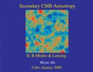
<strong>Secondary</strong> <strong>CMB</strong> <strong>Anisotropy</strong><br />
I: <strong>Reionization</strong><br />
<strong>Wayne</strong> Hu<br />
Cabo, January 2009
Outline<br />
Cabo Lectures (not all inclusive!)<br />
• <strong>Reionization</strong><br />
• B-modes<br />
Gravitational Lensing<br />
• Cosmic Acceleration<br />
Recent Reviews<br />
Primary and <strong>Secondary</strong> <strong>Anisotropy</strong>: Hu & Dodelson ARAA 40<br />
171 (2002)<br />
Lensing:Lewis & Challinor Phys Rep. 429 1 (2006)<br />
<strong>Secondary</strong> <strong>Anisotropy</strong>:Aghanim, Majumdar, Silk Rep. Prog.<br />
Phys. 71 066902 (2008)<br />
<strong>Reionization</strong>:Zaldarriaga et al, <strong>CMB</strong>pol White Paper (2008)
Outline<br />
Cabo Lectures (not all inclusive!)<br />
• <strong>Reionization</strong><br />
• B-modes<br />
Gravitational Lensing<br />
• Cosmic Acceleration<br />
Recent Reviews<br />
• Primary and <strong>Secondary</strong> <strong>Anisotropy</strong>: Hu & Dodelson ARAA 40<br />
171 (2002)<br />
• Lensing: Lewis & Challinor Phys Rep. 429 1 (2006)<br />
• <strong>Secondary</strong> <strong>Anisotropy</strong>: Aghanim, Majumdar, Silk Rep. Prog.<br />
Phys. 71 066902 (2008)<br />
• <strong>Reionization</strong>: Zaldarriaga et al, <strong>CMB</strong>pol White Paper (2008)
Physics of <strong>Secondary</strong> Anisotropies<br />
SZ<br />
Primary Anisotropies<br />
Doppler<br />
ISW<br />
Vishniac<br />
Lensing<br />
Patchy rei.<br />
recombination<br />
z~1000<br />
reionization<br />
z~10<br />
acceleration<br />
z~1
∆T (µK)<br />
100<br />
10<br />
1<br />
0.1<br />
Scattering Secondaries<br />
Doppler<br />
suppression<br />
density–mod<br />
linear<br />
ion-mod<br />
10 100 1000<br />
l<br />
SZ
∆T (µK)<br />
100<br />
10<br />
1<br />
0.1<br />
Gravitational Secondaries<br />
ISW<br />
lensing<br />
Moving Halo<br />
10 100 1000<br />
l<br />
un–<br />
lensed
<strong>Reionization</strong>
Across the Horizon<br />
Hu & White (2004); artist:B. Christie/SciAm; available at http://background.uchicago.edu
<strong>Anisotropy</strong> Suppression<br />
• A fraction τ~0.1 of photons rescattered during reionization out of<br />
line of sight and replaced statistically by photon with random<br />
temperature flucutuation - suppressing anisotropy as e -τ
Why Are Secondaries So Smalll?<br />
• Original anisotropy replaced by new secondary sources<br />
• Late universe more developed than early universe<br />
Density fluctuations nonlinear not 10 −5<br />
Velocity field 10 −3 not not 10 −5<br />
• Shouldn’t ∆T/T ∼ τv ∼ 10 −4 ?<br />
• Limber says no!<br />
• Spatial and angular dependence of sources contributing and<br />
cancelling broadly in redshift
Integral Solution<br />
• Formal solution to the radiative transfer or Boltzmann equation<br />
involves integrating sources across line of sight<br />
• Linear solution describes the decomposition of the source S (m)<br />
ℓ<br />
with its local angular dependence and plane wave spatial<br />
dependence as seen at a distance x = Dˆn.<br />
• Proceed by decomposing the angular dependence of the plane<br />
wave<br />
e ik·x = <br />
(−i) ℓ 4π(2ℓ + 1)jℓ(kD)Y 0<br />
ℓ<br />
• Recouple to the local angular dependence of G m ℓ<br />
G m ℓs<br />
ℓ<br />
ℓsℓ<br />
ℓ (ˆn)<br />
<br />
= (−i) ℓ 4π(2ℓ + 1)α (m) m<br />
(kD)Yℓ (ˆn)
Integral Solution<br />
• Projection kernels (monopole, temperature; dipole, doppler):<br />
ℓs = 0, m = 0 α (0)<br />
0ℓ ≡ jℓ<br />
ℓs = 1, m = 0 α (0)<br />
1ℓ ≡ j′ ℓ<br />
• Integral solution: for Θ = ∆T/T<br />
Θ (m)<br />
ℓ (k, 0)<br />
2ℓ + 1 =<br />
• Power spectrum:<br />
Cℓ = 2<br />
π<br />
∞<br />
0<br />
dk<br />
k<br />
<br />
−τ<br />
dDe<br />
<br />
m<br />
ℓs<br />
k3 〈Θ (m)∗<br />
ℓ<br />
Θ(m)<br />
ℓ 〉<br />
(2ℓ + 1) 2<br />
S (m)<br />
ℓs α(m)<br />
ℓsℓ (kD)<br />
• Solving for Cℓ reduces to solving for the behavior of a handful of<br />
sources. Straightforward generalization to polarization.
•<br />
•<br />
<strong>Anisotropy</strong> Suppression and Regeneration<br />
Recombination sources obscured and replaced with secondary<br />
sources that suffer Limber cancellation from integrating over<br />
many wavelengths of the source<br />
Net suppression despite substantially larger sources due to<br />
growth of structure except beyond damping tail
<strong>Reionization</strong> Suppression<br />
• Rescattering suppresses primary temperature and polarization<br />
anisotropy according to optical depth, fraction of photons rescattered
1.25<br />
1.20<br />
1.15<br />
1.10<br />
1.05<br />
1.00<br />
0.95<br />
0.90<br />
Tilt-τ Degeneracy<br />
• Only anisotropy at reionization (high k), not isotropic temperature<br />
fluctuations (low k) - is suppressed leading to effective tilt for WMAP<br />
(not Planck)<br />
Spergel et al (2006)<br />
WMAP1 (T)<br />
WMAP3 (T+E)<br />
WMAP1ext<br />
0.1 0.2 0.3 0.4 0.5
Doppler Effect
∆T (µK)<br />
100<br />
10<br />
1<br />
0.1<br />
Scattering Secondaries<br />
Doppler<br />
suppression<br />
density–mod<br />
linear<br />
ion-mod<br />
10 100 1000<br />
l<br />
SZ
(2l+1)j l (100)<br />
Doppler Effect in Limber Approximation<br />
• Only fluctuations transverse to line of sight survive in Limber approx<br />
but linear Doppler effect has no contribution in this direction<br />
d<br />
observer<br />
0<br />
0<br />
j Y0 l(kd)Yl Temperature Doppler<br />
l<br />
(2l+1)j l '(100)<br />
observer<br />
l<br />
d<br />
0<br />
0<br />
j Y<br />
l(kd)Yl 1
Cancellation of the Linear Effect<br />
<strong>Reionization</strong> Surface<br />
e— velocity redshifted γ<br />
overdensity<br />
Observer<br />
Cancellation<br />
blueshifted γ
<strong>Reionization</strong> Surface<br />
Modulated Doppler Effect<br />
e— velocity unscattered γ<br />
overdensity,<br />
ionization patch,<br />
cluster...<br />
Observer<br />
blueshifted γ
Ostriker–Vishniac Effect<br />
Doppler<br />
Primary<br />
Ostriker–<br />
Vishniac<br />
see Shirley Ho's talk<br />
Hu & White (1996)
Inhomogeneous Ionization<br />
• As reionization completes, ionization regions grow and fill the<br />
space<br />
Zahn et al. (2006) [Mortonson et al (2009)]
Inhomogeneous Ionization<br />
• Provides a source for modulated Doppler effect that appears<br />
on the scale of the ionization region
Patchy <strong>Reionization</strong><br />
Aghanim et al (1996)<br />
Gruzinov & Hu (1998)<br />
Knox, Scocciomarro<br />
& Dodelson (1998)
<strong>Secondary</strong> Polarization
WMAP Correlation<br />
• <strong>Reionization</strong> polarization first detected in WMAP1 through<br />
temperature cross correlation at an anomalously high value<br />
(l+1)C l/2π (µK 2 )<br />
3<br />
2<br />
1<br />
0<br />
-1<br />
0<br />
<strong>Reionization</strong><br />
10 40 100 200 400 800 1400<br />
Multipole moment (l)<br />
TE Cross Power<br />
Spectrum
Polarization from Thomson Scattering<br />
• Differential cross section depends on polarization and angle<br />
dσ<br />
dΩ<br />
= 3<br />
8π |ˆε ′ · ˆε| 2 σT<br />
dσ<br />
dΩ<br />
= 3<br />
8π |ˆε ′ · ˆε| 2 σT
Polarization from Thomson Scattering<br />
• Isotropic radiation scatters into unpolarized radiation
Polarization from Thomson Scattering<br />
• Quadrupole anisotropies scatter into linear polarization<br />
aligned with<br />
cold lobe
Whence Quadrupoles?<br />
• Temperature inhomogeneities in a medium<br />
• Photons arrive from different regions producing an anisotropy<br />
Hu & White (1997)<br />
hot<br />
cold<br />
hot<br />
(Scalar) Temperature Inhomogeneity
<strong>CMB</strong> <strong>Anisotropy</strong><br />
• WMAP map of the <strong>CMB</strong> temperature anisotropy
Whence Polarization <strong>Anisotropy</strong>?<br />
• Observed photons scatter into the line of sight<br />
• Polarization arises from the projection of the quadrupole on the<br />
transverse plane
Polarization Multipoles<br />
• Mathematically pattern is described by the tensor (spin-2) spherical<br />
harmonics [eigenfunctions of Laplacian on trace-free 2 tensor]<br />
• Correspondence with scalar spherical harmonics established<br />
via Clebsch-Gordan coefficients (spin x orbital)<br />
• Amplitude of the coefficients in the spherical harmonic expansion<br />
are the multipole moments; averaged square is the power<br />
E-tensor harmonic<br />
l=2, m=0
Modulation by Plane Wave<br />
• Amplitude modulated by plane wave → higher multipole moments<br />
• Direction detemined by perturbation type → E-modes<br />
Scalars<br />
π/2<br />
Polarization Pattern Multipole Power<br />
1.0<br />
0.5<br />
B/E=0<br />
φ l
A Catch-22<br />
• Polarization is generated by scattering of anisotropic radiation<br />
• Scattering isotropizes radiation<br />
• Polarization only arises in optically thin conditions: reionization<br />
and end of recombination<br />
• Polarization fraction is at best a small fraction of the 10 -5 anisotropy:<br />
~10 -6 or µK in amplitude
l(l+1)/2π Cl (µK 2 )<br />
WMAP 3yr Data<br />
100.00<br />
10.00<br />
1.00<br />
0.10<br />
WMAP 3yr: Page et al. 2006<br />
0.01<br />
1 10 100 1000<br />
l (multipole moment)
Temperature Inhomogeneity<br />
• Temperature inhomogeneity reflects initial density perturbation<br />
on large scales<br />
• Consider a single Fourier moment:
Locally Transparent<br />
• Presently, the matter density is so low that a typical <strong>CMB</strong> photon<br />
will not scatter in a Hubble time (~age of universe)<br />
recombination<br />
transparent<br />
observer
Reversed Expansion<br />
• Free electron density in an ionized medium increases as scale factor<br />
a -3; when the universe was a tenth of its current size <strong>CMB</strong> photons<br />
have a finite (~10%) chance to scatter<br />
recombination<br />
rescattering
Polarization <strong>Anisotropy</strong><br />
• Electron sees the temperature anisotropy on its recombination<br />
surface and scatters it into a polarization<br />
recombination<br />
polarization
Temperature Correlation<br />
• Pattern correlated with the temperature anisotropy that generates<br />
it; here an m=0 quadrupole
Instantaneous <strong>Reionization</strong><br />
• WMAP data constrains optical depth for instantaneous models<br />
of τ=0.087±0.017<br />
• Upper limit on gravitational waves weaker than from temperature
Why Care?<br />
• Early ionization is puzzling if due to ionizing radiation from normal<br />
stars; may indicate more exotic physics is involved<br />
• <strong>Reionization</strong> screens temperature anisotropy on small scales<br />
making the true amplitude of initial fluctuations larger by e τ<br />
• Measuring the growth of fluctuations is one of the best ways of<br />
determining the neutrino masses and the dark energy<br />
• Offers an opportunity to study the origin of the low multipole<br />
statistical anomalies<br />
• Presents a second, and statistically cleaner, window on<br />
gravitational waves from the early universe
Distance Predicts Growth<br />
• With smooth dark energy, distance predicts scale-invariant<br />
growth to a few percent - a falsifiable prediction<br />
Mortonson, Hu, Huterer (2008)
Ionization History<br />
• Two models with same optical depth τ but different ionization<br />
history<br />
ionization fraction x<br />
1.0<br />
0.8<br />
0.6<br />
0.4<br />
0.2<br />
0<br />
fiducial<br />
Kaplinghat et al. (2002); Hu & Holder (2003)<br />
5<br />
z<br />
step<br />
10 15 20 25
Distinguishable History<br />
• Same optical depth, but different coherence - horizon scale<br />
during scattering epoch<br />
l(l+1)C l EE /2π<br />
10 -13<br />
10 -14<br />
fiducial<br />
step<br />
Kaplinghat et al. (2002); Hu & Holder (2003)<br />
10 100<br />
l
Transfer Function<br />
• Linearized response to delta function ionization perturbation<br />
Tℓi ≡ ∂lnCEE ℓ<br />
, δC<br />
∂x(zi)<br />
EE<br />
ℓ = C EE<br />
<br />
ℓ Tℓiδx(zi)<br />
Transfer function<br />
Hu & Holder (2003)<br />
0.4<br />
0.2<br />
0<br />
∆z=1<br />
z i=8<br />
l<br />
z i=25<br />
i<br />
10 100
Principal Components<br />
• Eigenvectors of the Fisher Matrix<br />
Fij ≡ <br />
(ℓ + 1/2)TℓiTℓj = <br />
δx δx<br />
Hu & Holder (2003)<br />
ℓ<br />
0.5<br />
0<br />
-0.5<br />
0.5<br />
0<br />
-0.5<br />
(a) Best<br />
(b) Worst<br />
10 15<br />
µ<br />
Siµσ −2<br />
µ Sjµ<br />
z<br />
20 25
Capturing the Observables<br />
• First 5 modes have the information content and most of<br />
optical depth<br />
Hu & Holder (2003)<br />
10 2<br />
10 1<br />
1<br />
10 -1<br />
10 -2<br />
10 -3<br />
10 -4<br />
10 -5<br />
σ µ<br />
τ µ<br />
5 10 15<br />
mode µ<br />
prior
Representation in Modes<br />
• Truncation at 5 modes leaves a low pass filtered of ionization<br />
history<br />
• Ionization fraction allowed to go negative (Boltzmann code<br />
has negative sources)<br />
x<br />
Hu & Holder (2003)<br />
0.8<br />
0.6<br />
0.4<br />
0.2<br />
0<br />
10 15 20 25<br />
z
Representation in Modes<br />
• Reproduces the power spectrum with sum over >3 modes<br />
more generally 5 modes suffices: e.g. total τ=0.1375 vs 0.1377<br />
l(l+1)C l EE /2π<br />
Hu & Holder (2003)<br />
10 -13<br />
10 -14<br />
x<br />
0.8<br />
0.4<br />
0<br />
10 15 20 25<br />
true<br />
sum modes<br />
fiducial<br />
z<br />
10 100<br />
l
Total Optical Depth<br />
• Optical depth measurement unbiased<br />
• Ultimate errors set by cosmic variance here 0.01<br />
• Equivalently 1% measure of initial amplitude, impt for dark energy<br />
10 2<br />
10 1<br />
1<br />
10 -1<br />
10 -2<br />
10 -3<br />
10 -4<br />
10 -5<br />
σ µ<br />
σ τ (cumul.)<br />
5 10 15<br />
Hu & Holder (2003) mode µ<br />
τ µ<br />
prior<br />
prior
WMAP5 Ionization PCs<br />
• Only first two modes constrained, τ=0.101±0.017<br />
Mortonson & Hu (2008)
Model-Independent <strong>Reionization</strong><br />
• All possible ionization histories at z
Large Scale Anomalies
Large Angle Anomalies<br />
• Low planar quadrupole aligned with planar octopole<br />
• More power in south ecliptic hemisphere<br />
• Non-Gaussian spot<br />
NEP<br />
dipole<br />
EQX<br />
NSGP<br />
-0.019 0.000 0.019<br />
T (mK)<br />
EQX<br />
dipole<br />
SEP<br />
NEP<br />
SSGP<br />
dipole<br />
EQX<br />
NSGP<br />
-0.051 0.000 0.051<br />
T (mK)<br />
EQX<br />
dipole<br />
NEP<br />
dipole<br />
EQX<br />
NSGP<br />
-0.034 0.000 0.034<br />
T (mK)<br />
SEP<br />
SSGP<br />
EQX<br />
dipole<br />
SEP<br />
SSGP<br />
Copi et al (2006)
Polarization Tests<br />
• Matching polarization anomalies if cosmological<br />
Dvorkin, Peiris, Hu (2007)
Polarization Bumps<br />
• If features in the temperature spectrum reflect features in the<br />
power spectrum (inflationary potential), reflected in polarization<br />
with little ambiguity from reionization<br />
Mortonson et al (2009)<br />
Covi et al (2006)<br />
ionization adjusted<br />
to max/min feature
Summary: Lecture I<br />
• <strong>Reionization</strong> suppresses primary anisotropy as e −τ so the precision<br />
of initial normalization and growth rate measurements depends on<br />
τ precision<br />
• In temperature spectrum, suppression acts on small scalesand<br />
looks like tilt for WMAP (not Planck)<br />
• Linear Doppler effect highly suppressed on small scales, leading<br />
order term is modulated effect: OV, kSZ, patchy reionization<br />
• Rescattering of quadrupole anisotropy leads to linear polarization<br />
at large angles<br />
• Shape of polarization spectrum carries sufficient information to<br />
measure τ independently of ionization history (through PCs)<br />
• If large angle anomalies are cosmological, they will be reflected in<br />
polarization