t - Bentham Science

ADVANCED APPROACH TO
MITIGATE MAGNETIC FIELDS
AND YOUR HEALTH
A Comprehensive Mathematical Modeling for
Mitigation of Magnetic Field
A.R. MEMARI

CONTENTS
Preface i
About the Author iii
Chapter 1. Exposure to Electromagnetic Fields 1
1.1. Electric and Magnetic Fields 1
1.2. Brain Cancer 5
1.3. Breast Cancer 6
1.4. Appliances 8
Chapter 2. Fundamental of Magnetic Field 9
2.1. Magnetic Field 9
2.2. Calculation of Magnetic Field 12
2.3. Mitigating Loop 13
2.4. Calculation of Mitigating Loop Impedance 16
2.5. Numerical Illustrations 18
Chapter 3. Fundamental Calculations of Auxiliary Loop Voltage 21
3.1. Loop Voltage 21
Chapter 4. Calculation of Mitigating Magnetic Field 26
4.1. Mitigating Magnetic Field 26
4.2. Mitigation at other Locations 30
4.3. Effect of Angular Frequency 30
Chapter 5. Geometrical Positions of Auxiliary Loop 33
5.1. Geometrical Locations and Magnetic Field 33
5.2. The Auxiliary Mitigating Magnetic Field 35
is Located Above the Power Line
5.3. Effect of the Altitude on the Fields 38
5.4. Effect of Point of Consideration 39
5.5. Comparing the Two Locations 45
5.6. Process of Mitigation 47
5.7. Auxiliary Loop is Placed Below the Line 47
5.8. Auxiliary Loop is Placed Above the Line 47
5.9. Discussions 50
Chapter 6. Magnetic Field and Delta Connections 51
6.1. Delta Configuration 51
6.2. Characteristics of the Magnetic Fields 53
6.3. Effect of Altitude 54
6.4. Relationship Between the Magnetic Fields 55
6.5. Contribution of Mitigation on other Points 58
Chapter 7. Bundled-Conductors Magnetic Field Calculations 60
7.1. Bundled Conductors 60

7.2. Calculation of Angular Frequency 62
7.3. Numerical Illustrations 64
7.4. Angular Frequency 64
7.5. Calculation of Loop Voltage 66
7.6. Unmitigated Magnetic Field 68
7.7. Numerical Illustrations 70
7.8. Mitigating Loop Impedance 72
7.9. Process of Mitigation 74
7.10. Variation of Fields 75
7.11. Effect of Mitigating Field on other Locations 76
7.12. Numerical Illustrations 77
Chapter 8. Bundled-Conductors Vs. Single Conductor per Phase 82
8.1 Comparative Illustrations 82
8.2 Process of Mitigation 83
Chapter 9. Auxiliary Loop – Ground Wire 85
9.1. Ground Wires 85
Chapter 10. Mitigating Loop at Ground Level 86
10.1. Ground Level 86
10.2. Calculation of Loop Voltage 87
10.3. Effect of Mitigation 88
10.4. Comparative Illustrations 90
Chapter 11. Magnetic Field of Vertically Installed Conductors 93
11.1. Vertically Arranged Conductors 93
11.2. Unmitigated Magnetic Field 94
11.3. Loop Voltage 94
11.4. Mitigating Field 96
11.5. Ground Level 97
References 100
Index 101

PREFACE
The main purpose of preparing this book is to share with the readers my 15 years of experience
which I have accumulated during my post doctoral research work and in the times that followed.
Attempts have been made to scrutinize each case and provide readers with detailed information
and also to demonstrate applicability of the developed procedure.
The author truly hopes that in reference with the scientific reports and epidemiological studies
establishing a correlation between exposure to magnetic fields and human’s health, this book
may be considered as a useful tool to protect health of mankind threatened by exposure to
magnetic fields.
Electricity has always contributed tremendous effects on the growth of our societies as well as
changing the way mankind has lived. Electricity has gone through a number of changes and has
always been challenged to meet the demands. As there is nothing to produce hundred percent
advantages, electricity also cannot be of exception.
Even though, in fully developed societies with switching off electricity, life comes to a complete
halt, but the hazardous effects of electricity on human’s health, especially those who are in direct
contact with electricity or operating equipments run by electricity must be deeply investigated
and steps must be taken to protect mankind against such fatal threat.
During the past decades, generation of electricity has gone through major changes and
consequently, there are numerous methods to develop electricity. Irrespective of how electricity
is generated, there is only one way to transport this energy, and that is through transmission line.
Electrical power transmission lines are installed between the power plant and a substation. Since
it is desired to deliver a large amount of power through a very long distance, transmission
normally takes place at high voltage. Redundant lines are provided so that power can be routed
from any power plant to any load center. The conductors, which are made of aluminum alloy and
reinforced with steel strands and are not provided with insulators require minimum clearance.
When electricity entered market, it used to be delivered at the same voltage as to be used by
houses and other electrical equipments, which in turn required different circuits and the distance
between the power plant and the consumers was kept restricted.
In order to increase the distance between towers, which results in reducing the cost of
transmission, clad steel wires and high towers are used. The number of towers per kilometer
distance can be reduced to as few as 6 towers. The longest high voltage transmission line, which
is installed in Republic of Congo, has a length of 1700 kilometers.
Engineers are always concerned about the power loss in transmission line. This loss, which is
dissipated as heat due to the resistance, is proportional to the surface area of the transmission line
conductors. Consequently, the smaller the surface area, the lower will be the loss due to heat
dissipation. However, at very high voltages, corona discharge losses become very large. With
high voltage transmission line, the voltage is stepped up at the generating station and then
i

ii
stepped down to the voltage needed by the distribution network. Such process increases the
transmission efficiency.
Voltages lower than 110 KV are considered as sub-transmission voltages, whereas voltages
above 230 KV are known as extra high voltage. A network of transmission lines, substations and
power plants is known as transmission grid.
Due to high cost of generation of electricity, a strong possibility exists to import the required
extra power in places where consumption of electricity is variable (due to hot summer and cold
winter).
A.R. Memari, Ph.D., P. Eng.

ABOUT THE AUTHOR
The author is a holder of Ph.D. degree in High Voltage Engineering and has been
engaged in Post Doctoral Research work at the University of Toronto, Toronto, Canada.
Dr. Memari has published numerous scientific papers in the area of magnetic field
associated with high voltage transmission line. His research findings have been utilized
worldwide. In addition to American inventors who have utilized his research findings for
their invention, Japanese Scientists have also proven the practical implementation of his
research works. Dr. Memari has also published a book related to Law and Ethics.
Dr. Memari is a full member of Association of Professional Engineers Ontario (Canada)
and a Professional Member of Ontario Society of Professional Engineers. He is also in
possession of a patent at Canadian Intellectual Property Office.
Title of Invention: “Implementation of Capillary in Generation of Electricity”.
Dr. Memari’s second patent, which deals with mitigation of magnetic field contributed by
household appliances, will be filed in the near future.
iii

Advanced Approach to Mitigate Magnetic Fields and Your Health, 1-8 1
Exposure to Electromagnetic Fields
Abstract: This chapter deals with the epidemiological reports, which associates
exposure to magnetic field and the risk of fatal diseases such as brain cancer, leukemia,
breast cancer, depression and miscarriage. In addition to exposure to magnetic field
associated with high voltage transmission lines, possible relationship between health
hazard and exposure to residential magnetic field such as electric blanket, hair dryer,
toaster and many more have also been discussed.
Occupational and non-occupational exposure to magnetic field and how an office
worker’s health may be in danger by sitting near to some office equipment have been
studied.
Finally, a relation between central nervous system cancer and environmental exposure
has been established. This study also establishes a possible relation between modern
equipments and heart attack.
1.1. Electric and Magnetic Fields
Electric and magnetic fields are products of power lines, industrial machineries and
electrical equipments, such as computers, electric blankets, electric clocks, table lamps,
hair dryers, televisions, microwaves and many more.
Electromagnetic field comprises two components known as electric field and magnetic
field, which are investigated separately in low-frequency rate and since electromagnetic
does not have enough energy to rupture molecular bonds, it is known as non- ionizing
radiation.
Electric fields are generated by voltage and its strength increases as the voltage is
increased. Its unit is volts per meter and could be present even when the electrical
equipment is turned off. Walls and trees can easily shield electric fields. Electric field can
easily cause electrically charged aerosols to oscillate and since our body is a good
conductor, electric field around our head is increased by a factor of 18.
Magnetic fields are products of flow of current in any conductor. It is directly
proportional to the current flowing through the conductor, but it is inversely proportional
to the distance from the conductor carrying the current. Magnetic field has a unit of gauss
or tesla. Since magnetic field is a direct product of current, it can be present as long as
current is flowing. Consequently, it vanishes the moment the electrical equipment is
turned off.
It is only magnetic field that has been found responsible to cause cancer, leukemia, and
other health hazard in children and adults.
Health problems related to exposure to magnetic field began in USSR for the first time in
1960. In the early stage, the researchers concentrated on electric field because high
voltage transmission lines are well capable to produce more current in our body rather
than magnetic field. But the research could not find any evidence relating human’s health
problem to electric field, they therefore focused on magnetic fields.
It was in 1979 when for the first time researchers established a relationship between
leukemia, tumors of the nervous system in the children living near high voltage
A.R. Memari (Ed.)
All rights reserved - © 2009 Bentham Science Publishers Ltd.
CHAPTER 1

2 Advanced Approach to Mitigate Magnetic Fields and Your Health A.R. Memari
transmission lines. These researchers noticed that these children had doubled or tripled
their risk of developing these diseases.
Hazardous effects of magnetic fields have become more visible in recent years and since
more data and evidence are available, public and politicians are more concerned about
this invisible radiation generated by transmission lines, electric wiring, household
appliances and substations.
ELF magnetic field can penetrate human body, resulting in malfunctioning of nerve and
muscle cells and therefore, in order to protect health of general public against this
invisible radiation, an international limit must be established.
A report by National Institute of Environmental Health Science suggests that due to
insufficient evidence associating exposure to magnetic field with health hazard, an
aggressive regulatory action cannot be taken.
It is a misleading to use job title as a surrogate for exposure in occupational exposure to
magnetic field. There exists a remarkable difference between the field survey exposure
and the actual level of magnetic field to which a person may actually be exposed. Even
though hospital workers are non-electrical workers, but they are in contact with
equipments such as diagnostic, monitoring equipment, visual display terminal,
photocopier and many more, which are well capable of producing high level of magnetic
field.
The instruments used by non- electrical workers can expose them to a high level of
magnetic field. For example, an electric drill is well capable of producing magnetic field
as high as 5000 mG close to its handle, while many electric utility workers could be
exposed to magnetic field of 2 mG. Even though, office workers are generally exposed to
low level of magnetic field, but the overall exposure to magnetic fields should not be
ignored. It is estimated that an office worker may be exposed to a magnetic fields as high
as 100 mG as the officer might be sitting near to some office equipment, such as
photocopier, which may last for a long period of time everyday.
The Institute of Electrical and Electronics Engineers also reports of association of
exposure to magnetic field generated by high voltage transmission lines and household
appliances and human’s health.
Threat relating magnetic field to health problem in the general public has encouraged
researchers and scientists to conduct further investigations.
Even though the available data is not sufficient to truly believe that magnetic field stands
as a major threat to human health, there is also no enough evidence to believe that
magnetic field does not stand as a major threat. In the past decades scientists and
researchers of numerous countries have been deeply involved in collecting more data and
evidence regarding association of several types of cancer with exposure to magnetic field.
There are still disagreements among researchers about level of safety of magnetic field
and whether magnetic field causes diseases or promotes them.

A.R. Memari Advanced Approach to Mitigate Magnetic Fields and Your Health 3
Effect of magnetic field can be detected at low level, but it may lose its effect as the level
is raised, but this effect reappears, as the level is moved to a higher level. Consequently,
level of safety of magnetic field has become a ground of further investigation and
research.
For the past decades, scientists have become more concerned about possible relationship
between health hazards in particular, cancer, leukemia, brain tumor, depression and
suicide, and exposure to residential magnetic field as well as that of the high voltage
transmission lines.
Even though, numerous studies in the past established a relationship between magnetic
field exposure and childhood leukemia, but collaboration between National Cancer
Institute and Children Cancer Group, resulted in finding little evidence linking exposure
to magnetic field to development of acute lymphoblastic leukemia in children under age
of 15. Also, these studies have not been able to establish a relationship between exposure
to magnetic field and children brain tumor.
National Cancer Institute reports that children living in houses with high level of
magnetic field did not have an increased risk of childhood acute lymphoblastic leukemia.
National Cancer Institute also indicates that children living near high voltage
transmission lines were not at greater risk of leukemia. However some studies indicate
that magnetic field above 0.4 μT increases risk of childhood leukemia, though some
researchers put this value at 0.3 μT. Surprisingly, some other research institutes put the
maximum allowable level of exposure at 100 μT and even at 1.6 mT, which are 250 and
4000 times higher than the level above which the risk of childhood leukemia has been
observed to be doubled.
Some evidence shows that exposure to magnetic field of as low as 0.1 μT could stand
harmful to our body. This level of magnetic field can easily be found in vicinity of high
voltage and low voltage transmission lines. Perry et al. suggests a 40% increase in suicide
risk above 0.1 μT.
In UK an advisory group reports that between 2 and 4 out of 500 cases of childhood
leukemia per year could be due to elevated magnetic fields.
In a research conducted about effect of magnetic field of distribution systems, showed
that children living near such systems have doubled their risk of cancer death, and some
other researchers have found association between childhood leukemia and household
exposure to magnetic field.
Contrary to the above findings, other scientists conclude that the danger may have been
exaggerated.
UK government has recently issued a moratorium on constructing houses and schools
within 60 meters of the existing high voltage transmission lines. It may soon (in some
countries) be required for public to install special devices to check on their household
magnetic field exposure.

2.1. Magnetic Field
Advanced Approach to Mitigate Magnetic Fields and Your Health, 9-20 9
Fundamental of Magnetic Field
Abstract: Electricity has gone through lots of changes since it has been in use. But, the
hazardous effects of high voltage transmission line magnetic field have always been of
deep concern to scientists. In this chapter, a mathematical modeling has been
established, by which a hundred percent mitigation at any point of consideration would
be achievable. The developed equations are also capable of producing simultaneous
reduction of magnetic field at other points within the center of the right-of-way.
First, a procedure to obtain the total magnetic field contributed by the three- phase high
voltage transmission line has been established and then the angular frequency at which
maximum magnetic field occurs is developed.
In order to achieve the mitigation, an auxiliary mitigating loop has been implemented
and the required equation to calculate the mitigating magnetic field is developed. The
optimum value of this loop impedance is set. Since the designed auxiliary mitigating
loop is of passive type, no especial feedback equipments are needed to compensate for
the changes of the load currents.
In order to illuminate the capability of the developed equations a flat configuration of
230 KV transmission line has been utilized.
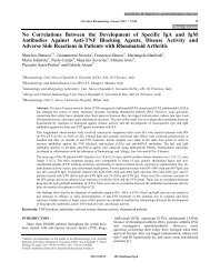
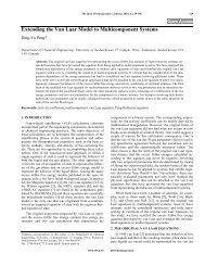
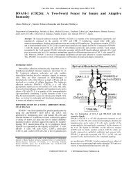
When a current carrying conductor is placed at point xi , y ( i ), it produces magnetic field
at point x j , y ( j ), which is directly proportional to current I , but it is inversely
proportional to the distance r ij as shown in Equation (1).
I
H ij =
ij () 1
2 * * r
ij
Where:
( ) 2
= cos
ij ( )+ sin( ) ( ) and r is the distance from the conductor to the point of
ij
consideration. is the angle that r makes with the vertical line h, as shown in Figure 1
ij
h
A B
K
Y
a a a
a b
c
K’
Figure 1. Position of the three phases with respect to an arbitrary point.
r
ij
C
K”
Ground level
A.R. Memari (Ed.)
All rights reserved - © 2009 Bentham Science Publishers Ltd.
CHAPTER 2
P X

10 Advanced Approach to Mitigate Magnetic Fields and Your Health A.R. Memari
Since current I is sinusoidal, the generated magnetic field also varies sinusoidally in
such manner that during positive half cycle its direction coincides with that of the
directional vector. It obtains an opposite direction during the negative half a cycle.
Equation (1) would have a trajectory of a circle if the directional vector was not included.
At distances beyond hundred meters from the transmission line, the effect of earth return
current must be considered. Such consideration, consequently requires a correction factor
to be added to Equation (1)
Since the currents in the transmission lines vary sinusoidally, the magnetic fields
produced by these currents, obviously, vary sinusoidally. The resultant magnetic field
vector is the vector sum of the magnetic field generated by each line, as expressed by
Equation (3). Sinusoidal variation of currents with respect to time and having a relative
phase displacement with respect to each other, the corresponding magnetic fields at the
point of consideration add up vectorially to produce the resultant magnetic field, T H .
H
T
= H
A
+ H
B
+ H
C
() 3
Where A B H
H , and C H are the magnetic fields produced by phase A, phase B and phase
C respectively. H A
, H B
and C H variations are sinusoidal along their own directions, but
due to phase displacement, there is a change with time not only in the magnitude of the
resultant vector HT but also in its orientation. These changes constitute the tip of
magnetic field vector HT to establish an ellipse, when angular frequency is allowed to
vary over 360°. Magnitudes and orientations of the major and minor axes are determined
by finding maximum and minimum points. The equation of this ellipse can be expressed
in terms of two orthogonal vectors.
The three sinusoidally varying currents are expressed as I A
, I B
and IC having a phase
difference of 120° and are depicted below.
I A = I
= I[
cos(
t
+ ) + j sin(
t
+ ) ]
I B = I(
120
) = I[
cos(
t
+ 120
) + j sin(
t
+ 120
) ]
I = I
+ 120 = I cos t
+ + 120 + j sin t
+ + 120 4
C
[ ]()
( ) ( ) ( )
Where t is angular frequency. The resultant magnetic field produced by the high
voltage transmission line at the point of consideration has four components, two real
components of X and Y and two imaginary components of X and Y as shown in Equation
(5)
H
T
=
( H + jH ) u + ( H + jH ) u () 5
rx
ix
x
ry
iy
y

A.R. Memari Advanced Approach to Mitigate Magnetic Fields and Your Health 11
The two real components of X and Y, Hrx and H , are responsible to establish the
ry
orientation in space. Variation of angular frequency over one complete cycle establishes
the locus of the magnetic field vector.
The three currents I A,
I B , I C are responsible to generate the induced voltage in the
mitigating loop. Consequently, the mitigating magnetic field is always proportional to the
three-phase current. Therefore, any changes in the value of these currents not only affect
the unmitigated magnetic field, but also the mitigating field. This effect occurs in such
proportionality that the resultant mitigated magnetic field remains unchanged.
Let us investigate the magnetic field generated by phase A. Since the real component of
the current is responsible to establish the orientation in space;
( t
)
[ cos(
) + i sin(
) ]() 6
I cos +
H A =
a a
2R
A
where; I is magnitude of the current in phase A. R A is the orthogonal distance from center
of phase A to the point of consideration. From Figure 1;
cos( a )= h
RA sin( a )= PK
R A
R A = sqrt PK
( ) 2
+ ( h)
2
( ) 7 ( )
The magnetic field produced by phase B is given by (8).
( t
+ 120
)
[ cos(
) + i sin(
) ]() 8
I cos
°
H B =
b b
2RB
From Figure 1;
cos( b)=
h
sin( b)=
R B
PK '
R B
R B = sqrt PK '
Similarly
( ) 2
+ ( h)
2
( )

Advanced Approach to Mitigate Magnetic Fields and Your Health, 21-25 21
CHAPTER 3
Fundamental Calculations of Auxiliary Loop Voltage
3.1. Loop Voltage
Abstract: Mitigating magnetic field is caused by the mitigating current in the auxiliary
mitigating loop. This current is achieved by dividing the mitigating loop voltage by the
mitigating loop impedance. The mitigating loop voltage is the result of the flux induced
by each phase of the three phases of the transmission line.
In this chapter, the flux induced by each phase has been thoroughly investigated and the
geometrical location of the auxiliary mitigating loop with respect to the power line has
been scrutinized and the related equations are established. The vector sum of these three
fluxes results in obtaining the total flux penetrating through the mitigating loop and the
corresponding equation is set. Finally, an equation to calculate the mitigating loop
voltage is developed. It is worth mentioning that phases A, B, and C are at 0°, -120° and
+120° respectively.
Loop voltage is the result of flux induced in a loop by a current carrying conductor. In
case of a three-phase transmission line, each phase induces its own flux in the loop
installed in vicinity of the power line. The vector sum of these three fluxes constitutes the
total flux induced by the transmission line.
Let us consider phase A;
r x
P
D
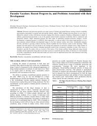
Figure 5. Two conductors forming a loop separated by a distance of D meters.
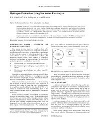
Figure 5 shows a loop formed by two conductors having radius of r separated by a
distance of D. Let P be any arbitrary point placed at a distance of x meters, as shown in
the same Figure.
Flux density B produced by current, I A
, of phase A has, at any instance, two
components, horizontal and vertical. It is the vertical component that penetrates through
the loop.
A.R. Memari (Ed.)
All rights reserved - © 2009 Bentham Science Publishers Ltd.

22 Advanced Approach to Mitigate Magnetic Fields and Your Health A.R. Memari
Accordingly;
D
A =
r
7
2*
10 * I A
. dx
x
( 19)
Figure 6. Induced flux in G1-G2 loop, when phase A is considered.
Figure 6 shows a loop made of two parallel conductors placed at an altitude of h meters
from a three-phase transmission line. ' indicates distance between point P and center of
phase A. ' makes an angle of with the vertical line AK. As this Figure shows, angle
can vary from ’ to ” and x = K’P.
x= KP – KK’
where; KP = h * tan()
and
KK ' = h *tan( ')
Substituting for the corresponding values in the above Equation;
() h * tan()
'
x = h * tan
as Figure 6 shows, angle is the only variable in the above Equation. Therefore,
derivative of this Equation with respect to angle results in;
dx = h*
1
( )
cos 2
d
G1 G2
K K’ P N
h m "
A
θ
'
θ
θ
ρ
'
B C

A.R. Memari Advanced Approach to Mitigate Magnetic Fields and Your Health 23
From the same Figure;
h = '*cos ( )
Substituting these values in Equation (19);
I A
A ( () ) d
' 7
2*
10 * 1
=
'* cos
2
'
' cos
After simplification;
A
=
2 * 10
7
*
I A
*
"
'
sin
cos
()
()
. d
()
Integration of the above Equation results in achieving the flux induced into the loop by
the current of phases A, as illustrated below.
A
=
Where:
I A
= I
2*
10
7
* I
A
*
[ cos ( t) + i * sin(
t)
]
[ ln(
cos()
' ) ln(
cos(
"
) ]( 20)
For the purpose of investigating contribution of current I B
of phase B to the same loop,
let us consider Figure 7.
G1 G2
x
K K’ P Q N
h m "
Figure 7. Induced flux in G1-G2 loop, when phase B is considered.
ρ
ϕ'
"
ϕ
A B C
ϕ

26 Advanced Approach to Mitigate Magnetic Fields and Your Health, 26-32
Calculation of Mitigating Magnetic Field
Abstract: A numerical illustration has been set up to demonstrate the applicability of
the developed equations to calculate the mitigating magnetic field. A point in the space
having a coordinate of (9, 1) has been selected as the point of consideration.
The total flux induced by the three phases of the transmission line is calculated, from
which the mitigating loop voltage is achieved. In order to achieve our attempt of
establishing a hundred percent cancellation of the magnetic field, optimal value of the
loop impedance is determined.
Variation of unmitigated magnetic field over one complete cycle in depicted and
simultaneous variation of unmitigated magnetic field and mitigated magnetic field is
also shown.
The influence of the mitigating magnetic field produced by the loop on the other
locations is also investigated and the results are tabulated. Effect of angular frequency
on producing magnetic field at other location is studied.
4.1. Mitigating Magnetic Field
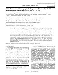
Mitigating magnetic field is one, which is produced by an auxiliary loop located either
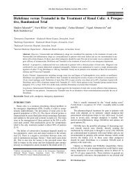
below or above the outer phases of a three-phase transmission line. Figure 9 shows the
case when the mitigating auxiliary loop is located beneath the line. The already existing
ground wires shown by G 1 and G 2 , in the Figures 6 through 8, could be used to also act
as a mitigating loop. Effectiveness of such a loop will be discussed in full details in the
coming chapter.
As was explained in the previous chapter, in order to achieve a hundred percent
cancellation of the unmitigated magnetic field, the magnetic field produced by the
auxiliary mitigating loop must be equal in magnitude to that of unmitigated field, but
opposite in direction. The auxiliary loop used for this purpose is of passive type, therefore
the flux induced by the three-phase currents is fully responsible to generate the mitigating
current in the mitigating loop. This is the advantage of having a passive loop, because
with changes in the load current not only the magnetic fields produced by the line is
affected, but also the mitigating current. Consequently, the resultant mitigated magnetic
field remains unchanged.
A
6 m
9 m
M 1
b
r
1 1
18 m
Figure 9. Geometrical location of mitigating loop with respect to point P.
Y
B
A.R. Memari (Ed.)
All rights reserved - © 2009 Bentham Science Publishers Ltd.
C
M 2
b 2
(0,1) P(9,1)
r
2
CHAPTER 4

A.R. Memari Advanced Approach to Mitigate Magnetic Fields and Your Health 27
For the illustrative purpose, a specific case has been analyzed. The mitigating loop is
located at 6 meters beneath the power line, as shown in Figure 9. Point P is the point of
consideration located at (9,1) from the center of right-of-way.
1
() ( ) 2
2
9 + 18
r =
= 20.1246
r
2
sin
=
cos
cos
sin
( )
( )
1
2 2 () 9 + () 0 = 9
1
( 2 ) =
( ) = 0
2
9
=
20.
1246
18
=
20.
1246
1
Implementation of Equation (16) requires us to determine the value of I m , which means
that the optimal value of the mitigating loop impedance Z m of Equation (18) must first be
obtained. All the parameters of Equation (18), but except V m , the mitigating loop voltage,
have already been determined. In order to calculate V m , let us apply Equations (20), (22),
(24), (25) and (26).
As shown in Figure 10;
A B C
Figure 10. Geometrical location of mitigating loop conductors with respect to the three phases.
Figure 10;
6 m
M 1
18 m
M 2

28 Advanced Approach to Mitigate Magnetic Fields and Your Health A.R. Memari
'=
0
a
" = 1.
2490
a
'
"
'
b
c
b
=
=
0.
9828
0.
9828
= 1.
2490
"
c = 0
I A = 460Amps
I = 460 * cos 120°
B
I C
A
B
C
=
=
=
460*
=
2*
10
2*
10
2*
10
[ ( ) + i * sin(
120°
) ]
[ cos(
120°
) + i * sin(
120°
) ]
7
* I A * [ ln(
cos(
'a
) ln(
cos(
"
a ) ]
7
* I B * [ ln(
cos(
'b
) ln(
cos(
"
b ) ]
7
* I * [ ln(
cos(
' ) ln(
cos(
"
) ]
C
c
c
The total flux penetrated by the three phases A, B and C would be the vector sum of the
three fluxes. Therefore;
T
and
m
=
A
+
B
+
V = 2000 * * 60 *
C
T
Therefore, for the considered case, the mitigating loop voltage would be equal to 69.1616
volts.
Since the main purpose of our attempt is to establish hundred percent cancellation of the
magnetic field, optimal value of the loop impedance, which is responsible to generate the
mitigating current in the mitigating loop, must be determined. Applying Equation (18)
and allowing angle ( ) = (
t)
, the value of the impedance for the given case would be
equal to Z m = 0.
3207 0.
0889i
. Implementation of Equation (16) sets the mitigating
magnetic field equal to H = 2
. 4406 + 2.
2023i.
m
The vector sum of unmitigated and mitigating magnetic fields results in the mitigated
magnetic field.
Variation of unmitigated magnetic field over one complete cycle is depicted in Figure 11.
This Figure shows that mitigating magnetic field forms the major axis of the unmitigated
field ellipse, which indeed justifies the previous explanations. As this Figure shows,
magnitude of mitigating magnetic field is equal to that of unmitigated magnetic field with
their orientations in opposite directions, resulting in a zero mitigated magnetic field. The

Advanced Approach to Mitigate Magnetic Fields and Your Health, 33-50 33
Geometrical Positions of Auxiliary Loop
Abstract: Effect of geometrical location of the auxiliary mitigating loop with respect to
the three phases of the transmission line is scrutinized. In this process, the mitigating
loop is first placed above and then below the two outer phases of the power line and a
comparative approach has been established. Positions of maximum and minimum values
of the mitigated magnetic fields with respect to the geometrical location of the loop are
also investigated. A 230 KV flat transmission line has been utilized and effect of
mitigation at the other points has also been studied.
Process of mitigation with respect to the geometrical location of the auxiliary loop and
the correlation between the three types of magnetic fields has also been studied and the
related figures and Tables are depicted.
5.1. Geometrical Locations and Magnetic Field
There are two elements that play very important role in producing magnetic field, current
and distance. In the case of mitigating magnetic field, in addition to these two elements
the altitude of the auxiliary mitigating loop from the three-phase transmission line and
also the separation between the two conductors shaping the auxiliary mitigating loop are
also immensely effective and should be thoroughly studied.
In order to illustrate effectiveness of geometrical location of the auxiliary mitigating loop
on mitigated magnetic field, two different locations, above and below the transmission
line, are selected and then at each location the mitigating loop is allowed to change its
altitude with respect to the power line.
TABLE 3. Effect of variations of mitigating loop altitude with respect to the power lines.
Distance from center of right-ofway.
Meters
-45 -36 -9 0 9 36 45
Unmitigated M.F. A/m 0.5249 0.7848 3.2874 3.7296 3.2874 0.7848 0.5249
h = 20 m 0.0350 0.0685 0.4158 0.000 0.4158 0.0685 0.0350
h = 10 m 0.0227 0.0468 0.2952 0.000 0.2952 0.0468 0.0227
h = 6 m 0.0165 0.0202 0.2092 0.000 0.2092 0.0355 0.0165
h =5 m 0.0149 0.0322 0.1818 0.000 0.1818 0.0322 0.0149
h =4m 0.0132 0.0287 0.1515 0.000 0.1515 0.0287 0.0132
h =3m 0.0114 0.0247 0.1181 0.000 0.1181 0.0247 0.0114
h =2m 0.0093 0.0197 0.0816 0.000 0.0816 0.0197 0.0093
h =1m 0.0060 0.0119 0.0425 0.000 0.0425 0.0119 0.0060
Mitigated Magnetic
Fields. A/ m
Figure 15 shows a schematic diagram of a 230 KV transmission line with its phases
separated by 9 meters. The mitigating loop is installed at 6 meters above the two outer
phases A and C. Let (0,1) be the point of consideration. As Table 2 shows, the angular
frequency responsible to generate maximum unmitigated magnetic field at (0,1) is equal
to 30 degrees.
Equation (10) is well applicable to determine the total unmitigated magnetic field
produced by this system at (0,1). From Figure 15;
A.R. Memari (Ed.)
All rights reserved - © 2009 Bentham Science Publishers Ltd.
CHAPTER 5

34 Advanced Approach to Mitigate Magnetic Fields and Your Health A.R. Memari
R A = sqrt 9
R B = 15m
R C = R A
cos( a )= 15
RA sin( a )= 9
( ) 2
+ ( 15)
2
( )
R A
cos( b)=
15
= 1
15
sin( b)=
0
cos( c )= 15
R C
sin( c )= 9
RC I = 450 Amps.
Therefore
H T
= -0.0000 - 3.6485i
= 17.4929m
Implementation of Equation (16) results in obtaining value of the mitigating magnetic
field.
Magnetic field A / m.
4
3.5
3
2.5
2
1.5
1
Unmitigated M.F.
0.5
Mitigated M.F.
h=10m
h=20m
0
-50 -40 -30 -20 -10 0 10 20 30 40 50
Distance from center of the right-of-way, meters
Figure 14. Contribution of altitude variation on mitigated magnetic field.

A.R. Memari Advanced Approach to Mitigate Magnetic Fields and Your Health 35
Case one;
5.2. The Auxiliary Mitigating Magnetic Field is Located at Above the Power Lines.
Figure 15. Schematic diagram of transmission line with mitigating loop M 1 M 2 .
From Figure 15;
r 1 = sqrt 9
r 2 = r 1
6 m
15 m
cos( 1)= 21
r1 ( ) 2
+ ( 21)
2
( )
( )= 9
sin 1 r1 cos( 2 )= 21
r2 M 1
A
1 m
b
sin( 2 )= 9
r2 V_loop = 69.1616 volts
Since, our aim is to create hundred percent cancellation of the unmitigated field,
= t
.
Implementation of Equation (18) results in achieving the optimal value of the loop
impedance Z m , from which I m is calculated. Substituting the above obtained values in
Equation (16)
H m
= 0.0000 + 3.6485i
1
a a
r
1
18 m
B
Y
RA RC
(0,1)
r
2
b
2
a c
M 2
C

Advanced Approach to Mitigate Magnetic Fields and Your Health, 51-59 51
Magnetic Field and Delta Connections
Abstract: In order to demonstrate the capability of the developed approach on any types
of transmission line, delta configuration power line has been investigated and numerical
illustration is established. The results are tabulated and the related figures are depicted.
In this chapter, characteristics of the magnetic fields and effect of the altitude of the
auxiliary mitigating loop with respect to the power line are studied. Finally, relationship
between the three types of the magnetic fields for delta – connected configuration has
been scrutinized and the depicted figure illuminates the discussions.
6.1. Delta Configuration
In order to demonstrate the capability of the established methods on other type of
configuration, a delta configuration power line will be considered.
Figure 28. A delta configuration with auxiliary mitigating loop installed beneath the two phases A and C.
4 m
G1 G2
B
4.3 m
27.4 m A C
16 m
6 m
A
2.5 m 2.5 m
1 M 2 M
Figure 28 shows delta – connected configuration. Table 7 shows the angular frequencies
at which maximum unmitigated magnetic fields corresponding to nine different locations
occur.
TABLE 7. Angular frequencies at which maximum unmitigated magnetic field is produced for a delta
configured power line.
Distance from center of the rightof-way.
Meters.
-10 -7.5 -5 -2.5 0 2.5 5 7.5 10
t, degrees 14.7 18 21.7 25.8 30 34.2 38.3 42 45.3
A.R. Memari (Ed.)
All rights reserved - © 2009 Bentham Science Publishers Ltd.
CHAPTER 6
20.3 m
1 m Ground level

52 Advanced Approach to Mitigate Magnetic Fields and Your Health A.R. Memari
A comparison between Table 2 and Table 7 shows that at the point of consideration
x j = 0 m, y j = 1m,
the angular frequencies, in both the cases, obtain the same value of
30°. These angular frequencies are responsible to produce maximum unmitigated
magnetic fields at those points.
In order to understand the reason, let us consider flat and delta configurations of Figures 3
and 28. It is obvious that parameters R A , R B and R C , are not the same, as shown in
Table 8.
TABLE 8. Relationships between parameters for two configurations
R A
R
R
B
C
Flat configuration Delta configuration
17.4929 15.2069
15 19.3000
17.4929 15.2069
Consequently, sine and cosine terms of Equation (11), in both the cases, would not be the
same.
For flat configuration: For delta configuration:
cos( a )= 0.8575
sin( a )= 0.5145
cos( b)=
1
sin( b)=
0
cos( c )= 0.8575
sin( c )= 0.5145
cos( a )= 0.9864
sin( a )= 0.1644
cos( b)=
1
sin( b)=
0
cos( c )= 0.9864
sin( c )= 0.1644
Substitution of the above parameters in Equation (11) for flat configuration results in
obtaining ; 0.0153 - 0.0255i as the numerator and -0.0088 - 0.0441i as denominator.
Whereas, substitution of the above parameter in Equation (11) for delta configuration
results in achieving: -0.0113 - 0.0094i as numerator and 0.0065 - 0.0162i as denominator.
Even though, in these two cases values of numerators and denominators are different, but
ratio of numerator to denominator in each case would be the same, constituting achieving
the value of 30°.
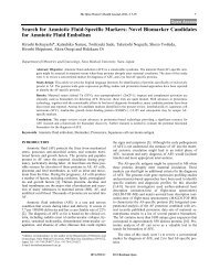
Figure 29 shows characteristics for the three types of magnetic fields for a delta -
connected configuration as shown in Figure 28 with x=0 m, y =1 m as point of
consideration.
The unmitigated magnetic field establishes an ellipse when the angular frequency is
allowed to vary over one complete cycle of 360˚. This Figure shows that mitigating

A.R. Memari Advanced Approach to Mitigate Magnetic Fields and Your Health 53
magnetic field forms the major axis and mitigated magnetic field shapes the minor axis of
this ellipse.
Real values of Y- components. A /m.
1.5
1
0.5
0
-0.5
-1
Unmitigated M.F.
Mitigated M.F.
Figure 29. Characteristics of the three magnetic fields. Delta-connection, -x=0, m, y1 m.
6.2. Characteristics of the Magnetic Fields
Mitigating M.F.
-1.5
-1 -0.8 -0.6 -0.4 -0.20 0.20.4 0.6 0.8 1
Real values of X-components A / m.
Variation of the three types of magnetic fields over one complete cycle of 360° is
depicted in Figure 30. As this Figure illustrates, the mitigated magnetic field achieves its
zero values at t equals to 30° and t equals to 210° respectively. At any value of angular
frequency between 30° and 210°, value of unmitigated magnetic field would not be the
same as that of mitigating magnetic field. Subsequently, values of mitigated magnetic
field within these values of angular frequencies would be greater than zero.
The unmitigated magnetic field fluctuates between a maximum value of 1.3709 A / m and
a minimum value of 0.9555 A /m. The mitigating magnetic field also varies between a
maximum value of 1.3709 A / m and a minimum value of zero as shown in Figure 30.
The mitigated magnetic field obtains its maximum value of 0.9555 A / m.
Relationship between the three magnetic fields for delta-connected power lines is exactly
the same as when the three phases are having the same y coordinates (flat configuration).
As Figure 30 reveals, the mitigated magnetic field after achieving its first zero value at
angular frequency of 30˚, increases until it reaches its maximum value of 0.9555 A / m,
which is equivalent to the minimum value of the unmitigated magnetic field, which
thereafter it declines until it obtains its zero value at angular frequency of 210˚.

60 Advanced Approach to Mitigate Magnetic Fields and Your Health, 60-81
CHAPTER 7
Bundled-Conductors Magnetic Field Calculations
Abstract: In this chapter, for further illumination of the developed approach to mitigate
magnetic field associated with high voltage transmission line, bundled-conductors
configuration has been scrutinized.
Each sub-conductor is separately analyzed and an equation to calculate the total
unmitigated magnetic field is achieved from which, angular frequency responsible to
generate maximum value of unmitigated magnetic field is set. An approach to calculate
the mitigating loop impedance is also established.
The applicability of the developed method has been illustrated and effect of mitigation
at seven different locations within the right-of-way has been thoroughly investigated.
Process of mitigation and variation of the three types of the magnetic fields with respect
to each other has been studied and the related figures and Tables are depicted.
7.1 Bundled Conductors
When voltage of a transmission line exceeds 230 KV, the effectiveness of corona
becomes more if only one conductor per phase is used. It is therefore preferred to utilize
more than one conductor per phase, which is known as bundling of conductors.
Therefore, a bundled conductor is one, which is made of two, three or even more
conductors, which are generally known as sub-conductors. These sub-conductors are
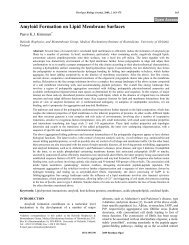
placed on a perimeter of a circle called bundle circle, as shown in Figure 35.
Figure 35. Bundled conductors.
The sub-conductors are placed much closer to one another as compared with the
separation of the three phases.
The relationship between sub-conductor spacing S and radius of bundle circle R is given
by S = 2 Rsin
, where n is number of sub-conductors.
n
In order to achieve minimum voltage gradient on the surface of a sub-conductor, the
optimum spacing between the sub-conductors must be carefully calculated, which is
usually eight to ten times the diameter of the conductor. Reduction of voltage gradient
results in radio interference reduction.
A.R. Memari (Ed.)
All rights reserved - © 2009 Bentham Science Publishers Ltd.

A.R. Memari Advanced Approach to Mitigate Magnetic Fields and Your Health 61
By bundling, GMD is obviously increased resulting in reduction of inductance L but
L
capacitance C increases, as a result the surge impedance, which is given by is
C
reduced. Therefore, maximum power that can be transmitted is increased.
Not only it is economically justified to use bundled conductors, but it also reduces
voltage gradient and interference with communication lines. The surge impedance is also
reduced by bundling the conductors.
1 m
Phase A
16 m
0.34 m
M1
G1 G2
4.5 m
Y
7.5 m
Figure 36. Bundled conductors with three sub-conductors on each phase.
Phase B Phase C
In order to illuminate the effectiveness of the developed methods on the bundled
conductors transmission line, a configuration as shown in Figure 36 is investigated.
As this Figure shows, each phase comprises three sub-conductors. These sub-conductors
are placed at a distance of 0.34 meters from each other. The total current of 510 Amps in
each phase is, obviously, equally divided among the three sub-conductors. Consequently,
each of the sub-conductors carries a current of 170 Amps. It is assumed that these three
phases are at 0, -120 and +120 degrees with respect to each other.
As has already been explained, the first step to calculate the maximum unmitigated
magnetic field contributed by this configuration is to determine the angular frequency.
Let us consider seven different locations, such as –13.5 m, -9 m, -4.5 m, 0 m, 4.5 m, 9 m,
and 13.5 m from the center of the right – of – way. It is also assumed that the object is
one meter above the ground level.
4.5m
10 m
M2
22 m
Ground Level X

62 Advanced Approach to Mitigate Magnetic Fields and Your Health A.R. Memari
7.2. Calculation of Angular Frequency
Considering each phase separately, unmitigated magnetic field produced by each subconductor
is calculated. The vector sum of these three magnetic fields results in obtaining
the magnetic field produced by each phase, at any point in the space. Then, the magnetic
field produced by each phase is vectorially added up, which results in obtaining the total
unmitigated magnetic field produced by this configuration.
Let the unmitigated magnetic field produced by the first sub-conductor of phase A be
H
, then
a1
I
=
cos
( t)
( cos(
) + i * sin(
)
a1
H a1
a1
a1
2ra1
Similarly, the unmitigated magnetic field H a2
sub-conductor are given by;
H
H
a2
a3
I
=
I
=
a2
a3
cos
2r
cos
2r
( t)
( cos(
) + i * sin(
) (
a2
( t)
( cos(
) + i * sin(
)
a3
a 2
a3
a2
a3
27)
and H a3
produced by the second and third
The three sub-conductors of phase B contribute unmitigated magnetic field as given by
(28)
H
H
H
b1
b2
b3
( t
120
)
( cos(
) + i * sin(
)
I b1
cos °
=
2rb1
b1
( t
120
)
( cos(
) + i * sin(
) )( 28)
I b2
cos °
=
2rb
2
b2
( t
120
)
( cos(
) + i * sin(
)
I b3
cos °
=
2rb
3
b3
Contribution of the three sub-conductors of phase C are given by (29)
H
H
H
c1
c2
c3
b1
b2
b3
( t
+ 120 )
( cos(
) + i * sin(
)
I c1
cos °
=
2rc1
c1
( t
+ 120 )
( cos(
) + i * sin(
) )( 29)
I c2
cos °
=
2rc
2
c2
( t
+ 120 )
( cos(
) + i * sin(
)
I c3
cos °
=
2rc
3
c3
c1
c2
c3

82 Advanced Approach to Mitigate Magnetic Fields and Your Health, 82-84
CHAPTER 8
Bundled-Conductors vs. Single Conductor per Phase
Abstract: A comparative illustration between a flat configuration of 230 KV single
conductor per phase and a bundled-conductor has been established. The obtained results
which, are tabulated show that the mitigated magnetic fields remain unchanged for both
the configurations.
8.1. Comparative Illustrations
Figure 46 shows a flat configuration of a 230 KV single conductor per phase transmission
line. Each of the three phases carries 510 Amps. This configuration is created to establish
a comparative illustration between a bundled-conductor transmission line of Figure 36
and a single conductor per phase. Let us also select the same locations, -13.5, -9, -4.5, 0,
4.5, 9, 13.5 meters.
Y
16 m
G 1
7.5 m
4.5 m 4.5 m
Figure 46. Flat configuration of a three phase transmission line.
Following similar procedures as was explained previously, the angular frequency
responsible to generate the maximum unmitigated magnetic field at the corresponding
location is calculated, the results of which are shown in Table 13.
G 2
A B C
M 1 M 2
Ground level
(0,1)
10 m
A.R. Memari (Ed.)
All rights reserved - © 2009 Bentham Science Publishers Ltd.
X

A.R. Memari Advanced Approach to Mitigate Magnetic Fields and Your Health 83
TABLE 13. Angular frequencies for a single conductor per phase
Distance d. Meters. Angular frequency. Degrees
-13.5 25.0320
-9 25.5583
-4.5 27.1996
0 29.9992
4.5 32.7989
9 34.4402
13.5 34.9665
Comparing Table 13 with Table 10, similar values of angular frequencies for the
corresponding distances from the center of right-of-way can be observed.
In order to establish a convincing explanation for the above phenomenon, let us scrutinize
Equation (33). From this Equation, it can be written that
( t) = M * cos(
t)
K * sin
therefore;
coefficient2
tan( t) =
=
coefficient1
M
K
Let us investigate location = 13.
5m
, = 1m
for the two configurations.
x j
y j
In the case of bundled conductors, implementation of Equations (34) and (35) result in
achieving
K = 1.3541 + i*0.2947
M = -0.6602 + i*0.0210
And in the case of single conductor per phase,
K = 1.3752 + i*0.2887
M = 0.6685 – i*0.0255
M
Consequently, the ratio of , generating the angular frequencies, in the two cases
K
remain very close to each other, resulting in obtaining very close values of angular
frequencies in both the cases.
8.2. Process of Mitigation
A close look at Table 12 and Table 14, it becomes obvious that even though a bundled-
conductor transmission line configuration differs from a single conductor per phase
configuration, but the mitigated magnetic fields remain almost unchanged.

84 Advanced Approach to Mitigate Magnetic Fields and Your Health A.R. Memari
TABLE 14. Relationship between distance and the two magnetic fields
Distance d. Meters -13.5 -9 -4.5 0 4.5 9 13.5
Unmitigated M.F. A/m 1.5493 2.0077 2.4139 2.5796 2.4139 2.0077 1.5493
Mitigated M.F. A/m 0.1119 0.1735 0.2579 0.3010 0.2701 0.0000 0.1368

Advanced Approach to Mitigate Magnetic Fields and Your Health, 85-85 85
Auxiliary Loop – Ground Wire
9.1. Ground Wires
Abstract: Effect of ground wire as an auxiliary mitigating loop has been investigated.
Since it is not feasible to provide the high voltage transmission lines with insulators to
protect them against the lightning, two conductors known as ground wires (in some cases
one) are directly installed above these lines. Ground wires are grounded at frequent
intervals, preferably at every pole. Ground wires cause a great reduction of dielectric
stress in the air, which could be due to lightning or other atmospheric disturbances. In
addition to station arresters, ground wire can act to dampen any impulses that may travel
along the transmission line. Therefore, more than protecting the lines, ground wires
provide a strong protection for the power station.
Since ground wires are placed along and parallel to the transmission lines, these two
conductors form a loop and, consequently, a voltage is induced in this loop.
Subsequently, the loop formed by the ground wires could be considered as a mitigating
loop.
The loop formed by the two conductors of the ground wires may well be capable to
produce hundred percent cancellation of magnetic field produced by the three-phase
transmission line. In such case, the loop impedance must be thoroughly studied and
optimal value of the impedance must be calculated. Such procedure, obviously, causes replacement
of the existing ground wires. Width of the loop will not cause any
inconvenience, since the developed method is well applicable to any rate of loop voltage.
Installation of an auxiliary mitigating loop above the transmission line may require height
of the tower to be increased. In addition, when auxiliary mitigating loop is placed above
the power lines, there will surely be a mutual effect between the mitigating loop and the
existing ground wires loop.
Readers are invited to thoroughly consider such mutual effect, if installation of an
auxiliary mitigating loop above a three-phase transmission line is desired.
A.R. Memari (Ed.)
All rights reserved - © 2009 Bentham Science Publishers Ltd.
CHAPTER 9

86 Advanced Approach to Mitigate Magnetic Fields and Your Health, 86-92
Mitigating Loop at Ground Level
Abstract: In order to demonstrate the feasibility of the developed approach, a case
when the mitigating loop is placed at the ground level is thoroughly studied. A flat
configuration of 230 KV transmission line has been used and effect of mitigation at
seven different locations within the right-of-way has been scrutinized and the related
figures and Tables are illustrated. The loop voltage, which is the result of induced
fluxes, is determined. Implementation of the previously derived equation results in
achieving the value of the mitigating loop impedance. The correlation between the three
types of magnetic fields has also been investigated. Finally, a comparative method when
the auxiliary mitigating loop is installed above, below and at the ground level is also
established and the result is shown in a Table.
10.1. Mitigating Loop at Ground Level
Figure 47 shows a flat configuration of a 230 KV transmission line with auxiliary
mitigating loop M 1 M 2 at the ground level.
Y
Figure 47. Geometrical position of mitigating loop M1 M with respect to point P.
2
Even though, this Figure illustrates that centers of the loop conductors are at the ground
level, but in practice and in order to safe guard the commuters against the electric shock,
this loop must be buried at a slight depth.
For the purpose of demonstrating the applicability of the developed approach, seven
locations such as -45, -36, -9, 0, 9, 36, and 45 meters from center of right-of-way are
selected. Let the object be placed at an altitude of 1 m above the ground level. Location
= 9m
, = 1m
is selected as the point of consideration.
x j
16 m
y j
9 m 9 m
A B C
M 1
q
j "
Ground level
j "
P (9,1)
The usual procedures are followed to calculate the unmitigated magnetic fields at these
locations.
y "
M 2
A.R. Memari (Ed.)
All rights reserved - © 2009 Bentham Science Publishers Ltd.
CHAPTER 10
1 m
X

A.R. Memari Advanced Approach to Mitigate Magnetic Fields and Your Health 87
10.2. Calculation of Loop Voltage
The three phases of the transmission line are well capable to induce fluxes in this loop.
The total flux, which is the vector sum of these three fluxes are responsible to generate
the loop voltage.
From Figure 47;
'
= 0
"
= 0.8442
I = 460 Amps
A
Substituting the above values in Equation (20), the flux induced by phase A is given by;
A
= 3.7626 e-005
Considering phase B;
'
= 0.
5124
"
= 0.
5124
I B
[ cos(
120°
) + * sin(
° ) ]
= 460 i 120
Substitution of the obtained values in Equation (22) results in achieving
B = 0
Considering phase C;
'
= 0.
8442
"
= 0
I C
[ cos(
120°
) + * sin(
° ) ]
= 460 i 120
From Equation (24);
C
= 1.
8813e
005
3.
2585e
005
i
Implementation of Equation (25) results in achieving the total flux induced in the
auxiliary mitigating loop. Therefore;
005
005
= 5.
6439e
3.
2585e
i
T
Finally, value of the loop voltage is determined by Equation (26).

Advanced Approach to Mitigate Magnetic Fields and Your Health, 93-99 93
CHAPTER 11
Magnetic Field of Vertically Installed Conductors
Abstract: In this chapter, vertically arranged conductors are investigated. The total
unmitigated magnetic field contributed by the three phases is calculated. The mitigating
loop voltage is calculated. This calculation reveals the fact that there will be no
mitigation when the auxiliary loop is installed symmetrically with respect to the Y-axis.
The capability of the developed approach is well illustrated once the loop’s geometrical
position is changed. The fluxes induced by the three phases of the power line are well
capable of producing mitigating loop voltage. Consequently, this voltage results in
achieving the mitigating magnetic field, Subsequently, the mitigated magnetic field is
calculated.
In order to further demonstrate the feasibility of the developed approach, the mitigating
loop is placed at the ground level and the related figures are depicted.
11.1. Vertically Arranged Conductors
Figure 53 shows a three-phase transmission line whose conductors are vertically
arranged. Phase A and phase B are separated by 9 meters and so are phases B and C.
Current in phase A is given by;
I A
= 460*
cos
( t)
Currents in phases B and C are, as shown below;
I
I
B
C
= 460 * cos
= 460 * cos
( t
120°
)
( t
+ 120°
)
This type of arrangement is well capable to produce magnetic field at any point in the
space. Since the generated magnetic field has sinusoidal variation, it obtains maximum
and minimum values
The angular frequency responsible to generate the maximum value of unmitigated
magnetic field at the point of consideration, x j = 9 m, y j = 1 m, contributed by this type
of arrangement can be calculated by implementing Equation (11).
From Figure 53;
R A = 17.4929 m
R
R
B
C
= 25.
6320m
= 34.
2053m
A.R. Memari (Ed.)
All rights reserved - © 2009 Bentham Science Publishers Ltd.

94 Advanced Approach to Mitigate Magnetic Fields and Your Health A.R. Memari
cos
sin
cos
sin
cos
sin
( a ) = 0.
8575
( a ) = 0.
5145
( b ) = 0.
9363
( b ) = 0.
5311
( c ) = 0.
9648
( ) = 0.
2631
c
Substitution of the above obtained values in Equation (11), sets value of the angular
frequency equal to 19.2 degrees.
1 m
16 m
Figure 53. Vertically arranged three-phase transmission line.
11.2. Unmitigated Magnetic Field
Equation (10) is well capable to calculate the total magnetic field contributed by this type
of arrangement. Substituting the already calculated values in Equation (10), sets value of
the unmitigated magnetic field equal to -1.3245 - 1.4196i, a magnitude of 1.9415 A / m.
11.3. Loop Voltage
6 m
C
9 m
B
Y
9 m Rc
A
Figure 53 also illustrates that a mitigating loop M 1 M 2 is installed beneath the three
conductors. Due to symmetrical arrangement of this auxiliary mitigating loop with
respect to Y-axis;
R B
M R A
1
18 m
M 2
P(9,1)
Ground level
X

Index Advanced Approach to Mitigate Magnetic Fields and Your Health, 2009 101
A
INDEX
Active circuit 13, 17
Acute lymphoblastic leukemia 3, 8
Adult leukemia 4, 5
Alzheimer 4
Altitude 39, 41, 42, 43
Angular frequency 10, 30, 32, 33, 49,
53, 60
Ampere’s Law 72
Amyotrophic lateral sclerosis 5
Appliances: 8
Association of exposure 2, 14
Auxiliary conductors 17
Auxiliary loop 13, 26,
Auxiliary loop impedance 87
Auxiliary mitigating loop 13, 17, 26, 33,
38, 42, 50
B
Brain Cancer 5
Brain tumor, 3, 5, 6
Breast Cancer 6, 7, 8
Bundled Conductors 59, 60, 70, 81, 82
Bundle circle 59
C
Calculation of Mitigating Loop 13
Cancer 2, 3, 4, 8
Children brain tumor 3
Children Cancer Group 4
Childhood leukemia, 3, 4, 5
Comparative 47, 81, 89,
Comparison 6, 7, 45, 52
Corona 17, 59
Current carrying conductor 9, 21
D
Delta configuration 51, 52
Depression 3, 4, 8
Dielectric stress 84
Discussions 50
Disease 5, 8
E
Earth return current 10
Effect of Altitude 38, 54
Effect of geometrical location 42
Effect of Mitigation 75, 87
Electric fields 1, 5
Electric and magnetic fields 1
Electrical equipments 1
Electromagnetic 1, 5
Ellipse 10, 28, 41, 53, 58
Epidemiological 5, 8
Environmental exposures 8
Environmental magnetic fields 6
Exposure to magnetic field 1, 2, 8
F
Flat configuration 18, 52, 53, 81
Flux density 21
Flux induced 21, 23, 38, 67, 86
G
Geometrical effect 56
Geometrical location 30, 33
Ground clearance 17, 89
Ground level. 85, 90
Ground wires 26, 84
H
Hazardous effects 1
Health hazard 1, 2
High voltage transmission lines. 1, 2
Household appliances and human’s
health. 1
Household appliances 1
Human’s health 1

102 Prepare Yourself For the Professional Practice Examination, 2009 A.R. Memari
I
Ice 17, 50, 89
Impedance 13, 16, 27, 28, 35, 95
Induced voltage 11, 37
L
Leukemia, 1, 3, 4, 6
Load current 13, 26
Loop voltage 11, 16, 21, 25, 37, 86,
93
Lymphoblastic 3, 8
M
Magnetic Field 9, 10, 11, 13
Magnetic field exposure 5
Major axis 28, 58
Maximum magnetic field 12
Maximum value. 38, 39, 47, 53, 56
Melatonin 6, 7
Minimum value 38, 39, 47, 53, 56
Minor axis 28, 58
Mitigated magnetic field 17, 28, 30,
37, 43, 53
Mitigating conductor 39
Molecular bonds 1
Mitigating loop 13, 26, 27, 28, 44, 65,
70
Mitigating current 13, 26, 37, 55
Mitigating loop impedance 16, 70
Mitigating magnetic field 26, 33, 34,
39, 43, 44, 49
Miscarriage 4
Musculoskeletal systems. 5
N
National Cancer Institute 3
Neurodegenerative disease. 5
Neurological diseases 4
Non- ionizing 1
Numerical Illustrations 18, 63, 69, 76
O
Occupational exposure 5, 6
Oncostatic 7
Orientation 10, 15, 16, 71, 74
Outer phases 17
P
Parkinson 5
Passive loop 13, 17, 42
Point of consideration. 10, 18, 30, 56,
58, 69, 70, 75, 87
Power lines 4, 33, 37, 45, 47
Pregnant women 4
Process of mitigation 47, 72, 82
R
Reproductive problems, 4
Residential magnetic field 3, 8
Right- of – way. 27, 32, 36, 45
S
Sub-conductors 59, 60, 61, 65, 67, 69
Suicide, 3, 4
Surge impedance 60
Symmetrically 30, 31
T
Tamoxifen. 7
Three-phase current 11, 13
Three-phase transmission line 21, 22,
26, 33
Transmission lines 2, 4, 13, 18, 42, 45,
70
Tumors 1, 3, 5
U
Unmitigated magnetic field 15, 28, 36,
53, 56, 67, 70
V
Vertically arranged conductors 92
Voltage gradient 59
W
Wind 17, 50
World Health Organization 4