

Radiative Transfer in Protoplanetary Disks
Radiative Transfer in Protoplanetary Disks
Radiative Transfer in Protoplanetary Disks

Create successful ePaper yourself
Turn your PDF publications into a flip-book with our unique Google optimized e-Paper software.
Introduction Activités Activités de de recherche recherche Projet Projet de de recherche recherche Résumé Résumé<br />
Un Un exemple exemple : IM : IMLup, Lup, une une CTTS CTTStypique typique<br />
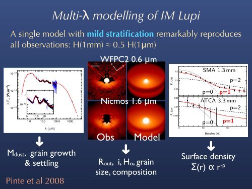
Multi-λ modell<strong>in</strong>g of IM Lupi<br />
Modélisation du dudisque disque d’IM Lup P<strong>in</strong>te et etal, al, 2008b, A&A<br />
!.F! (W.m−2 !.F! (W.m<br />
)<br />
−2 )<br />
A s<strong>in</strong>gle model with mild stratification remarkably reproduces<br />
all Un Un observations: unique modèle H(1mm) avec une une ≈ 0.5 faible H(1μm) stratification<br />
reproduit remarquablement bien l’ensemble des données<br />
WFPC2 bien l’ensemble 0.6 μm des données<br />
1’’<br />
E<br />
N<br />
1.0<br />
WFPC2 0.6 0.6 µm µm<br />
SMA SMA1.3 1.3mm mm<br />
10−12 10−12 10−14 10−14 2<br />
2<br />
10−16 10−13 10−16 10−13 5.<br />
5.<br />
10.0<br />
10.0<br />
20.<br />
20.<br />
1.0<br />
1.0<br />
10.0<br />
10.0<br />
100.0<br />
100.0<br />
1000.<br />
1000.<br />
! (µm) ! (µm)<br />
⇓⇓<br />
Mdisque, croissanceet<br />
Mdust,<br />
croissanceet<br />
gra<strong>in</strong> growth<br />
sédimentation<br />
& settl<strong>in</strong>g<br />
➜<br />
10 C. P<strong>in</strong>te et al.: Prob<strong>in</strong>g dust gra<strong>in</strong> evolution <strong>in</strong> IM<br />
1’’<br />
1’’<br />
E<br />
E<br />
N<br />
Nicmos<br />
Nicmos 1.6<br />
1.6<br />
Nicmos 1.6 µm µm<br />
μm<br />
Obs Modèles<br />
Model<br />
⇓<br />
F" (Jy)<br />
F" (Jy)<br />
F" (Jy)<br />
F" (Jy)<br />
0.2<br />
0.2<br />
0.1<br />
0.1<br />
0.05<br />
0.05<br />
0.02<br />
0.02<br />
0.01<br />
0.01<br />
0.005<br />
0.005<br />
p=0 p=0 p=1 p=1<br />
ATCA 3.3 3.3 mm mm<br />
p=2 p=2<br />
p=0 p=0<br />
0 50 100<br />
0 50 100<br />
Basel<strong>in</strong>e<br />
Basel<strong>in</strong>e<br />
(k!)<br />
(k!)<br />
p=2 p=2<br />
p=1 p=1<br />
⇓<br />
Densité de surface<br />
Σ(r) ∝ r −p<br />
⇓<br />
Densité de surface<br />
Σ(r) ∝ r −p<br />
Surface density<br />
Σ(r) α r-p Coll. Coll. Grenoble (Ménard, Augereau, Duchêne), JPL/Caltech (Padgett,Stapelfeldt),<br />
P<strong>in</strong>te et al 2008<br />
Arizona (Schneider), Leiden Leiden (Panić, van vanDishoeck), Dishoeck), Spitzer Legacy Team Teamc2d c2d<br />
N<br />
Brightness profile<br />
0.5<br />
0.0<br />
0 90 180 270<br />
Azimuthal angle ( o )<br />
Fig. 8. Scattered light images of the best models compared to observations. L<br />
at 0.606 µm andthelowerrowtothoseat1.6µm. Synthetic maps (right) w<br />
from theRext, peak). Rext, Central i, i, H0<br />
H0panel:<br />
0.6 µm azimuthalbrightnessprofile.Right<br />
central Rout, and right i, Ho, panels, gra<strong>in</strong> the red dashed l<strong>in</strong>e correspond to the best fit of the<br />
of all observations simultaneously and the blue dotted to the scatteredlight<br />
<strong>in</strong> the front side of the disc, i.e. towards bottom <strong>in</strong> the first panel.<br />
➜<br />
size, composition<br />
➜