Perturbative and non-perturbative infrared behavior of ...
Perturbative and non-perturbative infrared behavior of ...
Perturbative and non-perturbative infrared behavior of ...

Create successful ePaper yourself
Turn your PDF publications into a flip-book with our unique Google optimized e-Paper software.
Università degli Studi di Milano-Bicocca<br />
Facoltà di Scienze Matematiche, Fisiche e Naturali<br />
Dipartimento di Fisica G. Occhialini<br />
<strong>Perturbative</strong> <strong>and</strong> <strong>non</strong>-<strong>perturbative</strong> <strong>infrared</strong><br />
<strong>behavior</strong> <strong>of</strong> supersymmetric gauge theories<br />
Supervisor: Pr<strong>of</strong>. Silvia Penati<br />
External Referees:<br />
Pr<strong>of</strong>. Marialuisa Frau<br />
Pr<strong>of</strong>. Alex Sevrin<br />
Pr<strong>of</strong>. Kellog Stelle<br />
Doctoral Thesis <strong>of</strong>: Massimo Siani<br />
Dottorato di Ricerca in Fisica ed Astronomia (XXIII ciclo)
Riassunto della tesi<br />
L’accensione del Large Hadron Collider pone nuove sfide sulla presenza di nuova fisica oltre il<br />
Modello St<strong>and</strong>ard. Tra la pletora di modelli costruiti per spiegare i suoi risultati sperimentali,<br />
la supersimmetria è considerata la miglior c<strong>and</strong>idata tra tutta la nuova fisica che si potrebbe<br />
scoprire. La supersimmetria risolve la soluzione al problema della gerarchia, porta all’unificazione<br />
delle costanti di accoppiamento e contiene c<strong>and</strong>idati per la materia oscura.<br />
La miglior c<strong>and</strong>idata per una teoria consistente di gravità quantistica è la teoria di stringa.<br />
Le teorie di campo supersimmetriche e la teoria delle stringhe sono intimamente connesse. I gradi<br />
di libertà principali nella teoria delle stringhe sono stringhe vibranti i cui estremi sono vincolati<br />
ad oggetti estesi detti brane. La teoria di bassa energia con supporto su un insieme di brane<br />
coincidenti è una teoria supersimmetrica di Yang-Mills. Quindi è molto importante studiare il<br />
comportamento delle teorie di gauge supersimmetriche per capire di più sulla teoria delle stringhe.<br />
Una completa comprensione del limite di bassa energia delle teorie di gauge <strong>non</strong> è semplice,<br />
perché le teorie quantistiche di campo sono spesso fortemente accoppiate nel loro limite infrarosso.<br />
Tuttavia, la supersimmetria ci permette di conoscere molto sulle teorie efficaci di bassa energia.<br />
La prima parte di questa tesi studia un modello in cui la supersimmetria è parzialmente esplicitamente<br />
rotta mediante tecniche <strong>perturbative</strong> in superspazio N = 1. Il modello in considerazione<br />
sorge come limite di bassa energia di una configurazione della teoria di stringa in dieci dimensioni<br />
che rompe metà delle supercariche rompendo le regole di anticommutazione nell’algebra di<br />
supersimmetria. In questo modo solo una parte dei teoremi di <strong>non</strong>-rinormalizzazione vale ancora<br />
e l’invarianza di gauge e la rinormalizzabilita sono pr<strong>of</strong>ondamente legate tra loro. Nel formalismo<br />
ordinario la supersimmetria residua <strong>non</strong> è manifesta e ciò ha portato a conclusioni errate sulla<br />
proprietà di rinormalizzabilitá della teoria. Qui si discute di come il problema viene risolto in un<br />
formalismo manifestamente supersimmetrico. Si calcolano inoltre le funzioni beta della teoria a<br />
un loop e si trova che essa possiede alcuni punti fissi <strong>non</strong> banali. I flussi del gruppo di rinormalizzazione<br />
verso questi punti fissi possono essere studiati analizz<strong>and</strong>o attentamente la matrice di<br />
stabilitá in un loro intorno.<br />
La congettura AdS/CFT è una corrispondenza tra una teoria quantistica della gravità, come<br />
la stringa (o la M-) teoria, e una teoria di campo senza gravità in dimensione più bassa. Poiché<br />
la dualitá lega una teoria fortemente accoppiata con una debolmente accoppiata, i calcoli perturbativi<br />
nelle teorie di campo portano ad una maggiore comprensione di configurazioni fortemente<br />
accoppiate di teoria in stringa.<br />
Nella seconda parte della mia tesi ho applicato le tecniche <strong>perturbative</strong> del superspazio N = 1<br />
a teorie di campo in tre dimensioni. Queste descrivono il limite di bassa energia di un insieme<br />
di M2 brane coincidenti; le M2 brane sono i gradi di libertà fondamentali della M-teoria undici-
Riassunto della tesi<br />
dimensionale. Secondo la corrispondenza AdS/CFT, teorie tridimensionali di Chern-Simons supersimmetriche<br />
accoppiate con campi di materia sono la descrizione corretta di una particolare<br />
configurazione della M-teoria. Qui discutiamo una classe molto generale di teorie di Chern-Simons<br />
e le loro proprietá di rinormalizzazione e ricaviamo tutte le funzioni beta del modello. Quindi<br />
discutiamo i flussi del gruppo di rinormalizzazione e dimostriamo che tutti i punti fissi sono stabili<br />
nell’infrarosso. Questo è in pieno accordo con la AdS/CFT. Discutiamo inoltre l’insieme di<br />
operatori esattamente marginali ricavati dalle funzioni beta a due-loop.<br />
La spettro del Modello St<strong>and</strong>ard <strong>non</strong> è supersimmetrico, e quindi la supersimmetria, se esiste,<br />
deve essere rotta. Le sue principali caratteristiche sono mantenute solo se la rottura é spontanea,<br />
piuttosto che esplicita. Inoltre, è preferibile che il meccanismo di rottura di simmetria sia dinamico,<br />
perché in questo modo la scala elettrodebole viene esponenzialmente soppressa rispetto<br />
alla scala di cut-<strong>of</strong>f (che puó essere la scala di Planck o di gr<strong>and</strong>e unificazione), risolvendo così<br />
il problema della gerarchia. Sebbene la letteratura al riguardo sia vasta, <strong>non</strong> abbiamo ancora<br />
raggiunto una buona comprensione di questo problema.<br />
Un potente strumento <strong>of</strong>ferto dalla supersimmetria è la comprensione del regime di accoppiamento<br />
forte di una teoria di campo per mezzo di una dualità. In teorie di gauge supersimmetriche<br />
esiste una naturale dualitá elettrica/magnetica. Nella terza parte della tesi ci concentriamo sulle<br />
dualità in teorie N = 1 supersimmetriche, dette dualitá di Seiberg. Queste legano una teoria debolmente<br />
accoppiata con il limite di bassa energia di una teoria asintoticamente libera: é dunque<br />
un esempio di dualitá tra una teoria fortemente accoppiata e una debolmente accoppiata. Le<br />
proprietà <strong>non</strong>-<strong>perturbative</strong> della teoria microscopica possono essere calcolate perturbativamente<br />
nella teoria duale, o magnetica. Tramite la dualità di Seiberg, presentiamo un modello di rottura<br />
dinamica di supersimmetria che si basa su un’estensione della QCD supersimmetrica. Il limite<br />
di bassa energia di questa teoria è una teoria supersimmetrica di gauge fortemente accoppiata e<br />
il suo duale magnetico è debolmente accoppiato. Quindi i calcoli perturbativi sono affidabili, e<br />
discutiamo l’emergere di vuoti metastabili in cui la supersimmetria viene spontaneamente rotta, e<br />
di come la loro vita può essere resa più lunga della vita del nostro Universo. Inoltre, analizziamo<br />
un modello tridimensionale di rottura della supersimmetria, che é utile ad accrescere la nostra<br />
conoscenza della AdS/CFT e ad acquisire nuove conoscenze sulla gravità quantistica in quattro<br />
dimensioni.<br />
Nell’ultima parte della tesi discutiamo una recente applicazione della corrispondenza AdS/CFT.<br />
Alcuni fenomeni critici quantistici in sistemi della fisica dello stato solido sono ben descritti da<br />
teorie conformi fortemente accoppiate. Secondo la AdS/CFT, ad una determinata teoria conforme<br />
corrisponde una teoria classica di gravitá. Qui mostriamo come sia possibile costruire<br />
una teoria di gravità che descriva un modello di superconduttivitá e portare a termine un’analisi<br />
dettagliata delle sue caratteristiche.
Contents<br />
Contents i<br />
List <strong>of</strong> figures v<br />
Introduction <strong>and</strong> outline vii<br />
I Nonanticommutative theories 1<br />
1 Basics <strong>and</strong> motivations 3<br />
1.1 Introduction . . . . . . . . . . . . . . . . . . . . . . . . . . . . . . . . . . . . . . . . 3<br />
1.2 Nonanticommutativity from superstrings . . . . . . . . . . . . . . . . . . . . . . . . 4<br />
2 Nonanticommutative superspace 9<br />
2.1 Minkowski . . . . . . . . . . . . . . . . . . . . . . . . . . . . . . . . . . . . . . . . . 9<br />
2.2 Euclidean . . . . . . . . . . . . . . . . . . . . . . . . . . . . . . . . . . . . . . . . . 10<br />
2.3 Non-renormalization theorems . . . . . . . . . . . . . . . . . . . . . . . . . . . . . . 13<br />
3 The Wess-Zumino model 15<br />
3.1 Superspace approach . . . . . . . . . . . . . . . . . . . . . . . . . . . . . . . . . . . 15<br />
3.1.1 Generalities . . . . . . . . . . . . . . . . . . . . . . . . . . . . . . . . . . . . 15<br />
3.1.2 One-loop divergencies . . . . . . . . . . . . . . . . . . . . . . . . . . . . . . 17<br />
3.2 An all loop argument . . . . . . . . . . . . . . . . . . . . . . . . . . . . . . . . . . . 20<br />
4 Gauge theories 23<br />
4.1 Supersymmetric gauge theories on N = 1/2 superspace . . . . . . . . . . . . . . . . 24<br />
4.2 Pure gauge theory . . . . . . . . . . . . . . . . . . . . . . . . . . . . . . . . . . . . 33<br />
4.2.1 Two–point function . . . . . . . . . . . . . . . . . . . . . . . . . . . . . . . 34<br />
4.2.2 Three–point function . . . . . . . . . . . . . . . . . . . . . . . . . . . . . . . 36<br />
4.2.3 Four–point function . . . . . . . . . . . . . . . . . . . . . . . . . . . . . . . 37<br />
4.2.4 (Super)gauge invariance . . . . . . . . . . . . . . . . . . . . . . . . . . . . . 38<br />
4.2.5 The renormalizable gauge action . . . . . . . . . . . . . . . . . . . . . . . . 39<br />
4.3 Renormalization with interacting matter . . . . . . . . . . . . . . . . . . . . . . . . 41<br />
4.3.1 One–loop divergences: The matter sector . . . . . . . . . . . . . . . . . . . 42<br />
i
CONTENTS<br />
4.3.2 The superpotential problem . . . . . . . . . . . . . . . . . . . . . . . . . . . 45<br />
4.3.3 The solution to the superpotential problem . . . . . . . . . . . . . . . . . . 46<br />
4.3.4 The most general gauge invariant action . . . . . . . . . . . . . . . . . . . . 47<br />
4.3.5 One–loop renormalizability <strong>and</strong> gauge invariance . . . . . . . . . . . . . . . 52<br />
4.4 An explicit case: the U(1) theory . . . . . . . . . . . . . . . . . . . . . . . . . . . . 60<br />
4.4.1 U∗(1) NAC SYM theories . . . . . . . . . . . . . . . . . . . . . . . . . . . . 61<br />
4.4.2 One flavor case: Renormalization <strong>and</strong> β–functions . . . . . . . . . . . . . . 63<br />
4.4.3 Three–flavor case: Renormalization <strong>and</strong> β-functions . . . . . . . . . . . . . 66<br />
4.4.4 Finiteness, fixed points <strong>and</strong> IR stability . . . . . . . . . . . . . . . . . . . . 69<br />
4.5 Summary <strong>and</strong> conclusions . . . . . . . . . . . . . . . . . . . . . . . . . . . . . . . . 75<br />
II Three-dimensional field theories 79<br />
5 N = 2 Chern-Simons matter theories 81<br />
5.1 The ABJM model . . . . . . . . . . . . . . . . . . . . . . . . . . . . . . . . . . . . 82<br />
5.2 Generalizations . . . . . . . . . . . . . . . . . . . . . . . . . . . . . . . . . . . . . . 83<br />
6 Quantization, fixed points <strong>and</strong> RG flows 87<br />
6.1 Quantization <strong>of</strong> N = 2 Chern–Simons matter theories . . . . . . . . . . . . . . . . 88<br />
6.2 Two–loop renormalization <strong>and</strong> β–functions . . . . . . . . . . . . . . . . . . . . . . 93<br />
6.2.1 One loop results . . . . . . . . . . . . . . . . . . . . . . . . . . . . . . . . . 93<br />
6.2.2 Two-loop results . . . . . . . . . . . . . . . . . . . . . . . . . . . . . . . . . 95<br />
6.3 The spectrum <strong>of</strong> fixed points . . . . . . . . . . . . . . . . . . . . . . . . . . . . . . 98<br />
6.3.1 Theories without flavors . . . . . . . . . . . . . . . . . . . . . . . . . . . . . 98<br />
6.3.2 Theories with flavors . . . . . . . . . . . . . . . . . . . . . . . . . . . . . . . 101<br />
6.4 Infrared stability . . . . . . . . . . . . . . . . . . . . . . . . . . . . . . . . . . . . . 104<br />
6.4.1 Theories without flavors . . . . . . . . . . . . . . . . . . . . . . . . . . . . . 105<br />
6.4.2 Theories with flavors . . . . . . . . . . . . . . . . . . . . . . . . . . . . . . . 107<br />
6.5 A relevant perturbation . . . . . . . . . . . . . . . . . . . . . . . . . . . . . . . . . 109<br />
III Supersymmetry breaking 113<br />
7 Basics <strong>and</strong> motivations 115<br />
7.1 The supertrace theorem . . . . . . . . . . . . . . . . . . . . . . . . . . . . . . . . . 115<br />
7.2 Non-renormalizable interactions . . . . . . . . . . . . . . . . . . . . . . . . . . . . . 118<br />
7.3 Mediating the supersymmetry breaking effects: an overview . . . . . . . . . . . . . 119<br />
7.4 R-parity <strong>and</strong> R-symmetry . . . . . . . . . . . . . . . . . . . . . . . . . . . . . . . . 120<br />
8 Supersymmetric QCD <strong>and</strong> Seiberg duality 123<br />
8.1 Generalities . . . . . . . . . . . . . . . . . . . . . . . . . . . . . . . . . . . . . . . . 123<br />
8.1.1 Supersymmetric Lagrangians . . . . . . . . . . . . . . . . . . . . . . . . . . 125<br />
8.1.2 The vacuum state . . . . . . . . . . . . . . . . . . . . . . . . . . . . . . . . 126<br />
8.2 Supersymmetric QCD . . . . . . . . . . . . . . . . . . . . . . . . . . . . . . . . . . 127<br />
ii
CONTENTS<br />
8.2.1 Lagrangian . . . . . . . . . . . . . . . . . . . . . . . . . . . . . . . . . . . . 127<br />
8.2.2 Nf = 0 . . . . . . . . . . . . . . . . . . . . . . . . . . . . . . . . . . . . . . 128<br />
8.2.3 Nf < Nc . . . . . . . . . . . . . . . . . . . . . . . . . . . . . . . . . . . . . . 129<br />
8.2.4 Nf ≥ 3Nc . . . . . . . . . . . . . . . . . . . . . . . . . . . . . . . . . . . . . 133<br />
8.2.5 3<br />
2 Nc < Nf < 3Nc . . . . . . . . . . . . . . . . . . . . . . . . . . . . . . . . . 133<br />
8.2.6 Duality . . . . . . . . . . . . . . . . . . . . . . . . . . . . . . . . . . . . . . 134<br />
8.2.7 Nc + 2 ≤ Nf ≤ 3<br />
2 Nc . . . . . . . . . . . . . . . . . . . . . . . . . . . . . . . 135<br />
8.2.8 Deformations . . . . . . . . . . . . . . . . . . . . . . . . . . . . . . . . . . . 135<br />
8.3 SQCD with singlets: SSQCD . . . . . . . . . . . . . . . . . . . . . . . . . . . . . . 136<br />
9 Non-supersymmetric vacua 139<br />
9.1 Generalities <strong>and</strong> basic examples . . . . . . . . . . . . . . . . . . . . . . . . . . . . . 140<br />
9.2 The ISS model . . . . . . . . . . . . . . . . . . . . . . . . . . . . . . . . . . . . . . 143<br />
9.3 Metastable vacua in the conformal window . . . . . . . . . . . . . . . . . . . . . . 150<br />
9.3.1 A closer look to the conformal window . . . . . . . . . . . . . . . . . . . . . 150<br />
9.3.2 Metastable vacua by adding relevant deformations . . . . . . . . . . . . . . 152<br />
9.3.3 General strategy . . . . . . . . . . . . . . . . . . . . . . . . . . . . . . . . . 158<br />
9.3.4 Discussion . . . . . . . . . . . . . . . . . . . . . . . . . . . . . . . . . . . . . 159<br />
9.4 Supersymmetry breaking in three dimensions . . . . . . . . . . . . . . . . . . . . . 160<br />
9.4.1 Effective potential in 3D WZ models . . . . . . . . . . . . . . . . . . . . . . 160<br />
9.4.2 Three dimensional WZ models with marginal couplings . . . . . . . . . . . 163<br />
9.4.3 The general case . . . . . . . . . . . . . . . . . . . . . . . . . . . . . . . . . 165<br />
9.4.4 Relevant couplings . . . . . . . . . . . . . . . . . . . . . . . . . . . . . . . . 168<br />
Conclusions 171<br />
Appendices 173<br />
A Mathematical tools 175<br />
A.1 Group theory conventions . . . . . . . . . . . . . . . . . . . . . . . . . . . . . . . . 175<br />
A.2 Useful integrals . . . . . . . . . . . . . . . . . . . . . . . . . . . . . . . . . . . . . . 176<br />
A.3 Notations <strong>and</strong> conventions in three-dimensional field theories . . . . . . . . . . . . 176<br />
B Feynman rules 179<br />
B.1 Feynman rules for the general action (4.3.124) . . . . . . . . . . . . . . . . . . . . . 179<br />
B.2 Feynman rules for the abelian actions (4.4.146) <strong>and</strong> (4.4.147) . . . . . . . . . . . . 185<br />
C Details on supersymmetry breaking computations 193<br />
C.1 The bounce action for a triangular barrier in four dimensions . . . . . . . . . . . . 193<br />
C.2 The renormalization <strong>of</strong> the bounce action . . . . . . . . . . . . . . . . . . . . . . . 196<br />
C.3 The bounce action for a triangular barrier in three dimensions . . . . . . . . . . . . 198<br />
C.4 Coleman-Weinberg formula in various dimensions . . . . . . . . . . . . . . . . . . . 200<br />
iii
List <strong>of</strong> Figures<br />
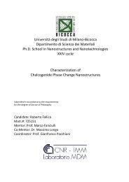
3.1 New vertices proportional to the external U superfield . . . . . . . . . . . . . . . . 17<br />
3.2 One-loop divergent diagrams with one insertion <strong>of</strong> the U(D 2 Φ) 3 -vertex . . . . . . . 18<br />
3.3 One-loop divergent diagrams with one insertion <strong>of</strong> the U(D 2 Φ) 2 -vertex . . . . . . . 19<br />
4.1 Gauge one-loop two-point functions. . . . . . . . . . . . . . . . . . . . . . . . . . . 34<br />
4.2 Gauge one-loop three-point functions. . . . . . . . . . . . . . . . . . . . . . . . . . 36<br />
4.3 Gauge one-loop four-point functions. . . . . . . . . . . . . . . . . . . . . . . . . . . 37<br />
4.4 One–loop two–point functions with chiral external fields. . . . . . . . . . . . . . . 44<br />
4.5 Master diagrams which, after the expansion <strong>of</strong> the covariant propagators, give rise<br />
to two, three <strong>and</strong> four–point divergent contributions. . . . . . . . . . . . . . . . . . 55<br />
4.6 Gauge self–energy diagram. . . . . . . . . . . . . . . . . . . . . . . . . . . . . . . . 63<br />
4.7 One–loop diagrams contributing to the mixed sector. . . . . . . . . . . . . . . . . 70<br />
4.8 One–loop diagrams contributing to the matter sector. . . . . . . . . . . . . . . . . 71<br />
4.9 Renormalization group trajectories near the h = ¯ h = 0 fixed point. Arrows indicate<br />
the IR flows. . . . . . . . . . . . . . . . . . . . . . . . . . . . . . . . . . . . . . . . 73<br />
6.1 One–loop diagrams for scalar propagators. . . . . . . . . . . . . . . . . . . . . . . . 93<br />
6.2 One–loop diagrams for gauge propagators. . . . . . . . . . . . . . . . . . . . . . . 94<br />
6.3 Two–loop divergent diagrams contributing to the matter propagators. . . . . . . . 95<br />
6.4 The exactly marginal surface <strong>of</strong> fixed points in the space <strong>of</strong> hi couplings, restricted<br />
to the subspace h1 = h2. The parameters have been chosen as K1 = 150,K2 =<br />
237,N = 43,M = 30. The dots denote the N = 3 <strong>and</strong> the N = 2, SU(2)A ×<br />
SU(2)B fixed points belonging to the ellipsoid. The plane represents the class <strong>of</strong><br />
theories (6.1.11) with SU(2) global symmetry <strong>and</strong> its intersection with the ellipsoid<br />
is the line described by (6.3.48). . . . . . . . . . . . . . . . . . . . . . . . . . . . . . 101<br />
6.5 Line <strong>of</strong> fixed points <strong>and</strong> RG trajectories. The arrows indicate flows towards the<br />
IR. We have chosen K = 100, N = 10, M = 20. . . . . . . . . . . . . . . . . . . . 105<br />
6.6 The ellipsoid <strong>of</strong> fixed points <strong>and</strong> the RG flows for N = 2 theories in the space <strong>of</strong><br />
couplings (h1 = h2,h3,h4). Arrows point towards IR directions. The parameters<br />
are K1 = 150, K2 = 237, M = 30 <strong>and</strong> N = 43. . . . . . . . . . . . . . . . . . . . . 107<br />
6.7 A sketch <strong>of</strong> the RG flow for the λi couplings only. A curve <strong>of</strong> fixed points is shown,<br />
which is IR stable. The red dot represents an isolated IR unstable fixed point.<br />
Here, the parameters are K1 = K2 = 20, M = N = 10, Nf = N ′ f = 1. . . . . . . . 108<br />
v
LIST OF FIGURES<br />
6.8 The three ellipses <strong>of</strong> fixed points <strong>and</strong> the RG flows for N = 2 theories with α<br />
couplings turned on. Arrows point towards IR directions. The parameters are<br />
K1 = K2 = 20, M = N = 10, Nf = N ′ f = 1. . . . . . . . . . . . . . . . . . . . . . 109<br />
6.9 RG trajectories on the h1 = 0 plane for N = 2 theories with α couplings turned<br />
on. Arrows point towards IR directions. The parameters are K1 = K2 = 20, M =<br />
N = 10, Nf = N ′ f = 1. . . . . . . . . . . . . . . . . . . . . . . . . . . . . . . . . . . 110<br />
6.10 RG trajectories for the flavored model with λi = 0 <strong>and</strong> equal <strong>non</strong>-vanishing α<br />
couplings. The arrows indicate flows towards the IR. We have chosen K1 = −K2 =<br />
100, M = N = 50, Nf = Nf ′ = 5. . . . . . . . . . . . . . . . . . . . . . . . . . . . 110<br />
9.1 ρ UV<br />
µ UV =10 −2 , Λc<br />
E UV = 10 −4 . . . . . . . . . . . . . . . . . . . . . . . . . . . . . . . . . . . . 157<br />
9.2 ρ UV<br />
µ UV =10 −4 , Λc<br />
E UV = 10 −4 . . . . . . . . . . . . . . . . . . . . . . . . . . . . . . . . . . . . 157<br />
9.3 ρ UV<br />
µ UV =10 −2 , Λc<br />
E UV = 10 −6 . . . . . . . . . . . . . . . . . . . . . . . . . . . . . . . . . . . . 157<br />
9.4 ρ UV<br />
µ UV =10 −4 , Λc<br />
E UV = 10 −6 . . . . . . . . . . . . . . . . . . . . . . . . . . . . . . . . . . . . 157<br />
9.5 ρ UV<br />
µ UV =10 −2 , Λc<br />
E UV = 10 −8 . . . . . . . . . . . . . . . . . . . . . . . . . . . . . . . . . . . . 157<br />
9.6 ρ UV<br />
µ UV =10 −4 , Λc<br />
E UV = 10 −8 . . . . . . . . . . . . . . . . . . . . . . . . . . . . . . . . . . . . 157<br />
9.7 One loop scalar potential for the one-loop validity region X < µ2<br />
4hf . Over this<br />
value, we find a classical runaway. At the origin the pseudo-modulus has negative<br />
squared mass. The potential is plotted for µ = 1, f = h = 0.1 . . . . . . . . . . . . 165<br />
B.1 Vertices from the action (4.3.124) at most linear in the NAC parameter F αβ . The<br />
(a,b,h,j)–vertices are order zero in ¯ θ, the (e)–vertex is proportional to ¯ θ ˙α whereas<br />
the remaining vertices are all proportional to ¯ θ 2 . . . . . . . . . . . . . . . . . . . . 186<br />
B.2 Vertices from the actions (4.4.146, 4.3.88). . . . . . . . . . . . . . . . . . . . . . . . 192<br />
C.1 Triangular potential barrier . . . . . . . . . . . . . . . . . . . . . . . . . . . . . . . 194<br />
vi
Introduction <strong>and</strong> outline<br />
The advent <strong>of</strong> the Large Hadron Collider poses new theoretical challenges on the physics beyond<br />
the St<strong>and</strong>ard Model. Among the plethora <strong>of</strong> models built to explain its experimental signatures,<br />
supersymmetry is considered the most compelling new physics that could be discovered. It addresses<br />
the solution to the hierarchy problem, leads to coupling constant unification <strong>and</strong> contains<br />
dark matter c<strong>and</strong>idates.<br />
The St<strong>and</strong>ard Model <strong>of</strong> particle physics successfully describes all the observed <strong>non</strong>-gravitational<br />
phenomena in the framework <strong>of</strong> quantum gauge theories, while gravity is described by Einstein’s<br />
General Relativity. Providing a framework in which quantum gravity <strong>and</strong> quantum gauge theories<br />
are described in a unified way is the dream <strong>of</strong> theoretical physics. The best c<strong>and</strong>idate<br />
for this would-be theory <strong>of</strong> everything is string theory. Consistency <strong>of</strong> string theory naturally<br />
dem<strong>and</strong>s that supersymmetry should be a symmetry <strong>of</strong> the spacetime we live in. While a deep<br />
underst<strong>and</strong>ing <strong>of</strong> string theory is far to be achieved, it is widely understood that supersymmetric<br />
field theories <strong>and</strong> string theory are intimately related. The main degrees <strong>of</strong> freedom in string<br />
theory are vibrating strings which can end on extended objects also called branes. The low energy<br />
theory living on a stack <strong>of</strong> branes is a supersymmetric Yang-Mills theory. Thus the physics <strong>of</strong><br />
string theory at long distances is well described by a supersymmetric local quantum field theory.<br />
Then it turns out that it is very important to underst<strong>and</strong> the <strong>behavior</strong> <strong>of</strong> supersymmetric gauge<br />
theories to learn more about string theory.<br />
A complete underst<strong>and</strong>ing <strong>of</strong> the low energy limit <strong>of</strong> gauge theories is not a simple task,<br />
because quantum field theories are <strong>of</strong>ten strongly coupled as they approach their <strong>infrared</strong> limit.<br />
Nevertheless, supersymmetry ensures better renormalization properties <strong>and</strong> a much more powerful<br />
<strong>non</strong>-<strong>perturbative</strong> analysis than ordinary quantum field theories. In other words, we can gain<br />
many insights on the <strong>behavior</strong> <strong>of</strong> the low energy effective theories if we allow supersymmetry to be<br />
a fundamental symmetry <strong>of</strong> Nature. This is the first step towards a deeper underst<strong>and</strong>ing <strong>of</strong> the<br />
same topics in theories with broken supersymmetries, with the ultimate goal <strong>of</strong> the application<br />
<strong>of</strong> similar techniques to ordinary field theories.<br />
The first part <strong>of</strong> my Thesis studies an explicit supersymmetry breaking model by means <strong>of</strong><br />
<strong>perturbative</strong> techniques in N = 1 superspace. The particular model arises as the low energy<br />
limit <strong>of</strong> a ten dimensional string theory background which breaks half <strong>of</strong> the supersymmetries by<br />
deforming the supersymmetry algebra down to a <strong>non</strong>-anticommuting one. In this setting only<br />
a subset <strong>of</strong> the <strong>non</strong>-renormalization theorems holds <strong>and</strong> the interplay <strong>of</strong> gauge invariance <strong>and</strong><br />
renormalizability is highly <strong>non</strong>trivial. In a component field formalism the residual supersymmetry<br />
is not manifest <strong>and</strong> this led to a wrong conclusion about the renormalizability property <strong>of</strong> the<br />
theory. I discuss how the problem is solved in a manifest supersymmetric setting. I also compute<br />
vii
Introduction <strong>and</strong> outline<br />
the β-functions <strong>of</strong> the theory to one-loop order <strong>and</strong> find they possess some <strong>non</strong>trivial fixed points.<br />
The RG flows towards these fixed points can be studied by carefully analyzing the stability matrix<br />
around them.<br />
The AdS/CFT conjecture is a remarkable correspondence between a quantum theory <strong>of</strong> gravity,<br />
such as string (or M-)theory, <strong>and</strong> a lower dimensional field theory without gravity. Because<br />
it is a weak/strong duality, <strong>perturbative</strong> field theories computations open the way to the underst<strong>and</strong>ing<br />
<strong>of</strong> strongly coupled string theoretical backgrounds <strong>and</strong> quantum gravity.<br />
In the second part <strong>of</strong> my Thesis I apply the <strong>perturbative</strong> techniques <strong>of</strong> N = 1 superspace<br />
to three-dimensional field theories. The latter have been shown to describe the low energy limit<br />
<strong>of</strong> a stack <strong>of</strong> M2 branes, the fundamental degrees <strong>of</strong> freedom <strong>of</strong> eleven-dimensional M-theory.<br />
By means <strong>of</strong> the AdS/CFT correspondence, supersymmetric three-dimensional Chern-Simons<br />
matter theories are the right description <strong>of</strong> M-theory in a particular background. I discuss in a<br />
very general setting the renormalization <strong>of</strong> Chern-Simons matter theories <strong>and</strong> present a complete<br />
treatment <strong>of</strong> their β-functions. Then I consider the RG flows <strong>and</strong> show that the fixed points are<br />
all <strong>infrared</strong> stable. This is in full agreement with the AdS/CFT conjecture. I also discuss the set<br />
<strong>of</strong> exactly marginal operators which arise at the two-loop level.<br />
The St<strong>and</strong>ard Model particle spectrum is not supersymmetric, <strong>and</strong> therefore supersymmetry,<br />
if it exists, must be broken. Its main features are preserved only if it is spontaneously broken,<br />
rather than explicitly broken. Furthermore, a dynamical symmetry breaking mechanism is<br />
preferred, because it triggers the electroweak scale to be exponentially smaller than the cut<strong>of</strong>f<br />
(Planck or gr<strong>and</strong> unified) scale, thus solving the hierarchy problem. Although many efforts have<br />
been made in this direction, a complete underst<strong>and</strong>ing <strong>of</strong> all these issues has not been achieved<br />
yet.<br />
A powerful tool <strong>of</strong>fered by supersymmetry is the underst<strong>and</strong>ing <strong>of</strong> the strong coupling regime<br />
<strong>of</strong> a field theory by means <strong>of</strong> dualities. In supersymmetric gauge theories there exists a natural<br />
electric/magnetic duality. In the third part <strong>of</strong> <strong>of</strong> my Thesis I concentrate on the N = 1 case,<br />
namely Seiberg duality. It relates a weakly coupled dual description <strong>of</strong> the low energy limit <strong>of</strong><br />
an asymptotically free theory, thus it is an example <strong>of</strong> a weak/strong duality. Non-<strong>perturbative</strong><br />
properties <strong>of</strong> the microscopic theory at low energies can be <strong>perturbative</strong>ly calculated in the dual<br />
magnetic theory. By the use <strong>of</strong> the Seiberg duality, I present a model <strong>of</strong> dynamical supersymmetry<br />
breaking based on an extension <strong>of</strong> the supersymmetric QCD. The low energy limit <strong>of</strong> this theory<br />
is a strongly coupled supersymmetric gauge theory <strong>and</strong> its magnetic dual is weakly coupled. Then<br />
the <strong>perturbative</strong> low energy computations are reliable, <strong>and</strong> I discuss how metastable vacua in<br />
which supersymmetry is broken are found, <strong>and</strong> how their lifetime can be made larger than the life<br />
<strong>of</strong> our Universe. I also analyze supersymmetry breaking in three dimensions, that should be useful<br />
to further explore the AdS/CFT correspondence <strong>and</strong> to gain new insights into four-dimensional<br />
quantum gravity.<br />
This Thesis is organized as follows. Part I is devoted to the study <strong>of</strong> <strong>non</strong>anticommutative<br />
field theories. In Chapter 1 we begin by discussing the starting motivations for the birth <strong>of</strong> the<br />
<strong>non</strong>anticommutative deformation as arising from string theory in the presence <strong>of</strong> a Ramond-<br />
Ramond flux. In Chapter 2 we construct the natural arena for the deformation, namely the<br />
viii
Introduction <strong>and</strong> outline<br />
<strong>non</strong>anticommutative superspace. We show how a suitable ∗-product can be obtained in the<br />
general superspace setup starting from the request for the most general structure compatible<br />
with the assumption <strong>of</strong> associativity. We also discuss the subtleties related to the right choice<br />
<strong>of</strong> complex conjugation rules, allowed only in Euclidean superspace, <strong>and</strong> we discuss the <strong>non</strong>renormalization<br />
theorems which hold due to the unbroken supersymmetry. A general discussion<br />
concerning the Wess-Zumino model is contained in Chapter 3. We discuss the quantum properties<br />
<strong>of</strong> the model up to two-loop, <strong>and</strong> give an all loop argument for its renormalizability. In Chapter<br />
4 we discuss in all details the case <strong>of</strong> gauge theories, both in the case <strong>of</strong> pure Super Yang-<br />
Mills theories <strong>and</strong> in the case <strong>of</strong> interacting matter. We develop a manifestly background gauge<br />
invariance method for computing loop corrections, by extending the background field method<br />
<strong>of</strong> ordinary supersymmetric theories. A complete one-loop analysis is carried out in all cases<br />
for <strong>non</strong>-Abelian unitary gauge groups. We conclude this Part by explicitly calculating all the<br />
β-functions for the Abelian gauge theory coupled to adjoint chiral superfields. We consider both<br />
the case with one chiral superfield <strong>and</strong> with three different flavors, thus our treatment includes<br />
the deformation <strong>of</strong> the N = 4 supersymmetric Yang-Mills theory. Although the Abelian N = 4<br />
theory is a free theory, we find that the <strong>non</strong>anticommutative deformation leads to a <strong>non</strong>trivial<br />
highly interacting action.<br />
In Part II we explain our results in three-dimensional field theories. Chapter 5 contains a<br />
basic description <strong>of</strong> three-dimensional field theories with a Chern-Simons term. Motivated by the<br />
AdS/CFT correspondence, we specialize to the case where the gauge group is the product <strong>of</strong> two<br />
unitary groups. In this class <strong>of</strong> theories, the maximally supersymmetric theory is conjectured to<br />
describe the dynamics <strong>of</strong> a stack <strong>of</strong> membranes probing a Calabi-Yau four-fold. The quantization<br />
<strong>of</strong> Chern-Simons theories coupled to matter fields is carried out in Chapter 6. We compute the<br />
two-loop β-functions <strong>and</strong> identify the fixed points <strong>of</strong> a large class <strong>of</strong> models. We study their<br />
<strong>infrared</strong> stability <strong>and</strong> their RG trajectories.<br />
Part III is devoted to supersymmetry breaking models. The basic material to relate them to<br />
the signatures <strong>of</strong> the visible (Supersymmetric) St<strong>and</strong>ard Model sector is explained in Chapter 7.<br />
In Chapter 8 we review the Supersymmetric Quantum Chromodynamics (SQCD), <strong>and</strong> show how<br />
supersymmetry allows us to compute exact, <strong>non</strong>-<strong>perturbative</strong>, quantum effects. The concept <strong>of</strong><br />
<strong>non</strong>-Abelian electric/magnetic duality is introduced, <strong>and</strong> we show that it is useful to describe the<br />
low energy dynamics <strong>of</strong> a supersymmetric gauge theory. While the low energy effective theory<br />
is <strong>of</strong>ten strongly coupled, its magnetic dual is weakly coupled. This allows us to use reliable<br />
perturbation theory <strong>and</strong> obtain calculable predictions on the <strong>non</strong>-holomorphic part <strong>of</strong> the theory.<br />
In particular, we show that SQCD possesses <strong>non</strong>-supersymmetric metastable vacua in Chapter 9.<br />
We compute the lifetime <strong>of</strong> the metastable vacua in the magnetic free range, <strong>and</strong> find they are long<br />
lived. We argue that this does not hold for the conformal window, because the RG flow combines<br />
the dimensionful parameters <strong>of</strong> the theory in such a way that the lifetime does not depend upon<br />
them. We overcome this problem by adding appropriate relevant deformations <strong>and</strong> show that a<br />
viable model <strong>of</strong> supersymmetry breaking can be realized in the conformal window. We end this<br />
Chapter by showing that supersymmetry breaking models also exist in three-dimensional field<br />
theories. The latter are a useful laboratory for the study <strong>of</strong> four-dimensional quantum gravity<br />
through the AdS/CFT correspondence.<br />
Some Appendices follow. In Appendix A we list our group theory <strong>and</strong> superspace conventions,<br />
both for four- <strong>and</strong> three-dimensional field theories. A list <strong>of</strong> useful integrals for evaluating the<br />
ix
Introduction <strong>and</strong> outline<br />
Feynman diagrams is also given. In Appendix B we collect the Feynman rules for <strong>perturbative</strong><br />
computations <strong>of</strong> <strong>non</strong>anticommutative theories. Details on supersymmetry breaking computations<br />
can be found in Appendix C.<br />
x
Part I<br />
Nonanticommutative theories<br />
1
Chapter 1<br />
Basics <strong>and</strong> motivations<br />
1.1 Introduction<br />
String theories naturally produce supersymmetric field theories as their low energy limits. Different<br />
configurations in string theory lead to different well-known field theories in the limit in<br />
which the string length shrinks to zero. For instance, the effective field theory on the worldvolume<br />
<strong>of</strong> N D3-branes in type IIB string theory compactified on a Calabi-Yau 3-fold is a N = 1<br />
U(N) supersymmetric Yang-Mills theory. Different amounts <strong>of</strong> supersymmetry can be obtained<br />
by changing the details <strong>of</strong> the configuration.<br />
Supersymmetric field theories can be defined on a superspace, where spacetime is enlarged<br />
by adding fermionic, i.e. anticommuting, coordinates. A remarkable discovery was the fact that<br />
string theory admits as its low energy limit a particular configuration in which the superspace<br />
coordinates algebra is modified. Considering a configuration <strong>of</strong> strings <strong>and</strong> branes in which a<br />
constant Ramond-Ramond self-dual graviphoton background field strength is turned on, in a<br />
suitable low energy limit the fermionic coordinates obey to the Clifford algebra<br />
<br />
θ α ,θ β<br />
= 2F αβ<br />
(1.1.1)<br />
with the remaining superspace structure unchanged [1]. Successively Seiberg began the study <strong>of</strong><br />
this kind <strong>of</strong> <strong>non</strong>anticommutative field theories [2] <strong>and</strong> since then a lot <strong>of</strong> work has been devoted<br />
to the study <strong>of</strong> the new peculiar effects <strong>of</strong> these models.<br />
First <strong>of</strong> all, we have strong constraints on the signature <strong>of</strong> the manifold: this deformation<br />
is only possible on Euclidean superspace. This is evident from constraints on the conjugation<br />
relations, but it is confirmed by its stringy origin. The low energy limit giving <strong>non</strong>anticommutative<br />
deformation in fact, is allowed because the self-dual graviphoton field is an exact solution<br />
to the string equation <strong>of</strong> motion (without backreaction): only in Euclidean space we can turn<br />
on the self-dual part while setting to zero the anti-self-dual one. Given the deformed structure<br />
<strong>of</strong> superspace, for <strong>non</strong>anticommutative field theories one has to define a Moyal ∗-product. It has<br />
to be defined by a fermionic differential operator <strong>and</strong>, starting from N = 1 supersymmetry, we<br />
have two different possibilities. By defining the ∗-product with covariant (with respect to the<br />
supersymmetry transformations) derivatives, we maintain all the supersymmetries <strong>of</strong> the theory,<br />
but a consistent definition <strong>of</strong> chirality can no more be given. Since the chirality is a fundamental<br />
3
1. Basics <strong>and</strong> motivations<br />
ingredient in building sensible supersymmetric field theories, this choice is not suitable for the<br />
N = 1 case. The second possibility is given by choosing the supercharges as generators <strong>of</strong> the<br />
∗-product. In this case, although chirality can be consistently defined, deformed field theories<br />
show a partially broken supersymmetry. In particular, if one starts from a N = 1 superspace, the<br />
resulting theories will have N = 1<br />
2 supersymmetry. Actually, one can try to give similar deformations<br />
also in superspace with extended supersymmetry: what happens is that more possibilities<br />
are involved. In the N = 2 case, for example, we can preserve the entire supersymmetry <strong>and</strong><br />
Euclidean group.<br />
The breaking <strong>of</strong> half <strong>of</strong> the supersymmetry has important consequences on the dynamics <strong>of</strong><br />
these field theories. In particular, since supersymmetry plays a fundamental role in determining<br />
the quantum properties <strong>of</strong> a field theory, the well known no-renormalization theorems are no<br />
longer valid, <strong>and</strong> a systematic analysis is compelling. The simple deformation <strong>of</strong> the original<br />
theories, obtained by trading the usual product with the Moyal one, is no longer renormalizable.<br />
However, the remaining unbroken supersymmetry preserves these models from the catastrophe,<br />
<strong>and</strong> a suitable completion <strong>of</strong> the action, with a finite number <strong>of</strong> new terms, is always possible<br />
in order to cure the divergences. Moreover, the new divergences arising from supersymmetry<br />
breaking for these theories maintain their logarithmic nature: this strongly suggests the fact that<br />
the breaking <strong>of</strong> the supersymmetry obtained in the string setup by turning on the flux <strong>of</strong> F αβ is<br />
a s<strong>of</strong>t breaking.<br />
1.2 Nonanticommutativity from superstrings<br />
In this section we show how the concept <strong>of</strong> <strong>non</strong>anticommutativity arises in string theory when<br />
a constant graviphoton background is considered. The four-dimensional theory is obtained by<br />
compactifying the ten-dimensional Type II superstring on a three-fold Calabi-Yau manifold [3,<br />
2, 4]. A similar derivation can be carried out for the full ten-dimensional superstring theory [5].<br />
In what follows, we make use <strong>of</strong> Berkovits’ formalism [6] which furnishes a very compact<br />
derivation. In this setup, the target-space supersymmetry <strong>of</strong> the superstring theory is manifest.<br />
Moreover, it allows for a covariant quantization <strong>of</strong> the superstring theory.<br />
The four-dimensional superspace coordinates the usual bosonic ones x µ <strong>and</strong> the fermionic θ α ,<br />
θ ˙α , ¯ θ α <strong>and</strong> ¯ θ ˙α . In our notations, a dot over an index indicates target space Weyl spinor chirality,<br />
while a bar indicates worldsheet holomorphicity. The relevant part <strong>of</strong> the Lagrangian density is<br />
(we set α ′ = 1)<br />
L = 1<br />
2 ∂xµ ¯ ∂xµ + pα ¯ ∂θ α + p ˙α ¯ ∂θ ˙α + ¯pα∂ ¯ θ α + ¯p ˙α∂ ¯ θ ˙α<br />
(1.2.2)<br />
where pα, ¯pα, p ˙α <strong>and</strong> ¯p ˙α are the conjugate momenta to the fermionic variables they couple to.<br />
Since we are working in the euclidean signature, they are independent variables. The worldsheet<br />
is parametrized by z <strong>and</strong> ¯z which are complex conjugate <strong>of</strong> each other.<br />
The Lagrangian (1.2.2) describes a free conformal field theory: all the fields satisfy free<br />
equations <strong>of</strong> motion, which are second order for the bosonic coordinates <strong>and</strong> first order for the<br />
fermionic ones. Moreover, the theory exhibits N = 2 target space supersymmetry. It is useful to<br />
define the worldsheet versions <strong>of</strong> the covariant derivatives dα <strong>and</strong> d ˙α <strong>and</strong> <strong>of</strong> the supercharges qα<br />
4
<strong>and</strong> q ˙α<br />
y µ = x µ + iθ α σ µ<br />
α ˙α θ ˙α + i ¯ θ α σ µ<br />
α ˙α ¯ θ ˙α<br />
1.2. Nonanticommutativity from superstrings<br />
d ˙α = p ˙α − iθ α σ µ<br />
α ˙α ∂xµ − 1<br />
2 θα θα∂θ ˙α + 1<br />
4 θ ˙α∂(θ α θα) (1.2.3)<br />
qα = −pα − iσ µ<br />
α ˙α θ ˙α ∂xµ + 1<br />
4 θ ˙α θ ˙α∂θα − 3<br />
4 ∂(θαθ ˙α θ ˙α) (1.2.4)<br />
<strong>and</strong> similarly for the others, in terms <strong>of</strong> which the Lagrangian density becomes<br />
L = 1<br />
2 ∂yµ ¯ ∂yµ − qα ¯ ∂θ α + d ˙α ¯ ∂θ ˙α − ¯qα∂ ¯ θ α + ¯ d ˙α∂ ¯ θ ˙α + total derivative (1.2.5)<br />
Therefore, q <strong>and</strong> d represent the conjugate momenta to the θ’s at fixed y exactly as the p’s<br />
represent the conjugate momenta at fixed x.<br />
If the worldsheet ends on a D-brane, the boundary conditions are easily found by imposing<br />
that there is no surface term in the equations <strong>of</strong> motion. For a boundary at z = ¯z, the boundary<br />
conditions are<br />
θ(z) = ¯ θ(¯z) q(z) = ¯q(¯z) d(z) = ¯ d(¯z) (1.2.6)<br />
which break half <strong>of</strong> the supersymmetries preserving only Qα + ¯ Qα <strong>and</strong> Q ˙α + ¯ Q ˙α.<br />
Now consider the system in the background <strong>of</strong> a constant graviphoton field strength Fαβ.<br />
Differently from the Lorentzian signature case, in euclidean signature we are allowed to take a<br />
self-dual field strength<br />
Fαβ = 0 F ˙α ˙ β = 0 (1.2.7)<br />
We take a self-dual F because such a background is a solution <strong>of</strong> the spacetime equations <strong>of</strong><br />
motion without backreaction <strong>of</strong> the metric. Indeed, a purely self-dual field strength does not<br />
contribute to the energy momentum tensor <strong>and</strong> therefore does not lead to a source in the gravity<br />
equations <strong>of</strong> motion. Moreover, since the kinetic term <strong>of</strong> the graviphoton does not contain the<br />
dilaton, the background Fαβ does not lead to a source in the dilaton equation.<br />
The graviphoton background is represented in the worldsheet Lagrangian by adding the interaction<br />
with the supersymmetry currents<br />
F αβ qα¯qβ<br />
(1.2.8)<br />
which makes manifest that the worldsheet theory remains free in this background. While the<br />
original coordinates x couple to F, the y’s remain free <strong>and</strong> independent <strong>of</strong> the background.<br />
The <strong>non</strong>trivial part <strong>of</strong> the Lagrangian now reads (we reinstate the right powers <strong>of</strong> α ′ )<br />
L = −qα ¯ ∂θ α − ¯qα∂ ¯ θ α + F αβ qα¯qβ<br />
The fields q <strong>and</strong> ¯q can be integrated out using their equations <strong>of</strong> motion<br />
¯∂θ α = α ′ F αβ ¯qβ<br />
∂ ¯ θ α = −α ′ F αβ qβ<br />
(1.2.9)<br />
(1.2.10)<br />
5
1. Basics <strong>and</strong> motivations<br />
to obtain the effective Lagrangian<br />
Leff =<br />
<br />
1<br />
α ′ <br />
∂<br />
F αβ<br />
¯ θ α¯ β<br />
∂θ<br />
(1.2.11)<br />
When we consider a system with a boundary (along z = ¯z for an euclidean worldsheet) we need<br />
to find the appropriate boundary conditions. These are determined from the surface term in the<br />
equations <strong>of</strong> motion<br />
<br />
1<br />
<br />
¯∂θ α<br />
δ¯β θ + ∂¯α β<br />
θ δθ<br />
F αβ<br />
<br />
z=¯z = 0 (1.2.12)<br />
Then, we impose<br />
θ α (z = ¯z) = ¯ θ α (z = ¯z)<br />
∂ ¯ θ α (z = ¯z) = − ¯ ∂θ α (z = ¯z) (1.2.13)<br />
The first condition states that the superspace has half the number <strong>of</strong> θ’s. This means that half<br />
<strong>of</strong> the supersymmetries has been broken. The second condition, through equation (1.2.10), that<br />
the supersymmetry charges qα <strong>and</strong> ¯qα are equal on the boundary.<br />
By imposing the proper singularity at coincident points, Fermi statistics <strong>and</strong> the aforementioned<br />
boundary conditions, we find the fermionic propagators<br />
〈θ α (z)θ β (ω)〉 = α′2 F αβ<br />
2πi<br />
〈 ¯ θ α (z) ¯ θ β (ω)〉 = α′2 F αβ<br />
2πi<br />
〈θ α (z)θ β (ω)〉 = α′2 F αβ<br />
2πi<br />
¯z − ω<br />
log<br />
z − ¯ω<br />
¯z − ω<br />
log<br />
z − ¯ω<br />
(z − ω)(¯z − ¯ω)<br />
log<br />
(z − ¯ω) 2<br />
(1.2.14)<br />
(1.2.15)<br />
Since the branch cuts <strong>of</strong> the logarithms are outside the worldsheet, for two points on the boundary<br />
z = ¯z ≡ τ <strong>and</strong> ω = ¯ω ≡ τ ′ we get<br />
corresponding to the algebra<br />
〈θ α (τ)θ β (τ ′ )〉 = α′2 F αβ<br />
2<br />
sign (τ − τ ′ ) (1.2.16)<br />
{θ α ,θ β } = α ′2 F αβ ≡ 2F αβ = 0 (1.2.17)<br />
which represents a Clifford algebra for the θ’s. It is important that since the coordinates ¯ θ <strong>and</strong><br />
y were not affected by the background coupling (1.2.8) they remain commuting. In particular<br />
[y, µ ,y ν ] = 0 <strong>and</strong> therefore [x µ ,x ν ] = 0 <strong>and</strong> [x,θ] = 0. This is also consistent with the purely field<br />
theoretical point <strong>of</strong> view (see [1] <strong>and</strong> the next chapter).<br />
It is easy to see that the Clifford algebra deformation breaks half <strong>of</strong> the supersymmetries<br />
left by the D-brane boundary conditions. Since the equation <strong>of</strong> motion <strong>of</strong> θ states that q is<br />
holomorphic, it extends to a holomorphic field ¯q(¯z) = q(z), <strong>and</strong> therefore the supersymmetry<br />
6
1.2. Nonanticommutativity from superstrings<br />
charge Qα + ¯ Qα is conserved. On the other h<strong>and</strong>, θ <strong>and</strong> ¯ θ are not holomorphic objects <strong>and</strong> do<br />
not extend to holomorphic fields through the boundary (because <strong>of</strong> (1.2.15)). Therefore, the<br />
supercharges Q ˙α + ¯ Q ˙α are broken by the deformation.<br />
As a final remark, note that the deformation (1.2.17) does not survive the field theory limit<br />
α ′ → 0 unless we simultaneously take F αβ → ∞ with α ′2 F αβ kept fixed. It is possible to make<br />
sense <strong>of</strong> this limit since the constant self-dual graviphoton background is an exact solution to the<br />
string equations <strong>of</strong> motion for any value <strong>of</strong> F αβ .<br />
7
1. Basics <strong>and</strong> motivations<br />
8
Chapter 2<br />
Nonanticommutative superspace<br />
As far as it is recognized that the symmetries play an important role in the study <strong>of</strong> the properties<br />
<strong>of</strong> a physical system, a formalism to make them linearly realized has becomed the key to<br />
simplify computations <strong>and</strong> gain more insights in the system at h<strong>and</strong>. As we are dealing with<br />
(partially) broken supersymmetries, we need a formalism which only makes manifest the survived<br />
supersymmetries. This is the <strong>non</strong>anticommutative superspace.<br />
In this section we analyze the basics <strong>of</strong> <strong>non</strong>(anti)commutative geometry, <strong>and</strong> look for the most<br />
general consistent four-dimensional superspace which realizes it. We consider the deformation<br />
<strong>of</strong> the Minkowski superspace, then we move to the euclidean case, which will be <strong>of</strong> much more<br />
interest for us. We conclude this section by giving the new (<strong>non</strong>)-renormalization theorems which<br />
arise in this context.<br />
2.1 Minkowski<br />
We start by considering the four-dimensional N = 1 Minkowski superspace. We denote by<br />
z A = (x αad ,θ α , ¯ θ ˙α ) the superspace coordinates, where x α ˙α are the four bosonic coordinates <strong>and</strong><br />
θ α , ¯ θ ˙α are the Weyl fermions which satisfy the conjugation rule (θ α ) † = ¯ θ ˙α . We deform the N = 1<br />
algebra given by<br />
{θ α ,θ β } = { ¯ θ ˙α , ¯ θ ˙ β } = {θ α , ¯ θ ˙α } = 0<br />
[x α ˙α ,θ β ] = [x α ˙α , ¯ θ ˙ β ] = 0<br />
[x α ˙α ,x β ˙ β ] = 0 (2.1.1)<br />
to the most general set <strong>of</strong> (anti)commutation relations<br />
<br />
θ α ,θ β<br />
= A αβ (x,θ, ¯ θ) ,<br />
<br />
¯θ ˙α<br />
, θ¯ β˙ = Ā ˙α ˙ β<br />
(x,θ, θ) ¯<br />
α<br />
θ , θ¯ ˙α = B α ˙α (x,θ, ¯ θ)<br />
<br />
x a ,θ β<br />
= iC aβ (x,θ, ¯ θ) ,<br />
<br />
x a , ¯ θ ˙ β <br />
= i ¯ C a ˙ β<br />
(x,θ, θ) ¯<br />
<br />
x a ,x b<br />
= iD ab (x,θ, ¯ θ) (2.1.2)<br />
9
2. Nonanticommutative superspace<br />
where A, B, C, D are functions <strong>of</strong> the superspace variables, Ā, ¯ C are the hermitian conjugates <strong>of</strong><br />
A <strong>and</strong> C respectively <strong>and</strong> ¯ B, ¯ D are hermitian operators.<br />
While the covariance under Lorentz transformation is manifest, we require (2.1.2) to be covariant<br />
under (super)translations<br />
θ ′α = θ α + ǫ α<br />
¯θ ′ ˙α = ¯ θ ˙α + ¯ǫ ˙α<br />
x ′α ˙α = x α ˙α + a α ˙α − i<br />
2<br />
ǫ α¯ θ ˙α + ¯ǫ ˙α θ α <br />
(2.1.3)<br />
which constraints the functional dependence <strong>of</strong> the functions A, B, C, D upon the coordinates.<br />
By performing a supertranslation on the coordinates (2.1.2) <strong>and</strong> computing the new algebra,<br />
one finds that A <strong>and</strong> B are independent <strong>of</strong> the coordinates <strong>and</strong> C <strong>and</strong> D are independent <strong>of</strong> the<br />
bosonic coordinates. More precisely, we get the algebra<br />
where<br />
<br />
θ α ,θ β<br />
<br />
x α ˙α ,θ β<br />
<br />
x α ˙α , ¯ θ ˙ β <br />
<br />
x α ˙α ,x β ˙ β <br />
= A αβ<br />
= iC α ˙αβ (θ, ¯ θ)<br />
= i ¯ C α ˙α ˙ β (θ, ¯ θ)<br />
,<br />
¯θ ˙α , ¯ θ ˙ β <br />
= Ā ˙α ˙ β<br />
, θ α , ¯ θ ˙α α ˙α<br />
= B<br />
= iD α ˙αβ ˙ β (θ, ¯ θ) (2.1.4)<br />
C α ˙αβ (θ, ¯ θ) = C α ˙αβ − 1<br />
2 θαB β ˙α − 1<br />
2 ¯ θ ˙α A αβ<br />
D α ˙αβ ˙ β<br />
(θ, θ) ¯ α ˙αβ<br />
= D ˙ β i<br />
−<br />
− i<br />
4<br />
2<br />
<br />
θ β ¯ C α ˙α ˙ β − ¯ θ ˙α C β ˙ βα − θ α ¯ C β ˙ β ˙α + ¯ θ ˙ βC α ˙αβ <br />
<br />
θ α Ā ˙α ˙ β θ β + θ α B β ˙α¯ θ ˙ β + ¯ θ ˙α B α ˙ β θ β + ¯ θ ˙α A αβ ¯ θ ˙ β <br />
<strong>and</strong> A, B, C <strong>and</strong> D are constant functions.<br />
2.2 Euclidean<br />
(2.1.5)<br />
In the Minkowski case it is impossible to break only half <strong>of</strong> the supersymmetries due to the<br />
conjugation rules <strong>of</strong> the spinorial variables. It is known that relaxing these constraints amounts<br />
to deal with extended supersymmetry or consider a space with euclidean signature. The main<br />
difference with respect to the Minkowski one relies on the reality conditions satisfied by the<br />
fermionic variables. In euclidean signature a reality condition on spinors is applicable only in the<br />
case <strong>of</strong> extended supersymmetry. The simplest case is then the N = 2 superspace.<br />
The spinors <strong>of</strong> the N = 2 euclidean superspace satisfy the pseudo-Majorana condition<br />
10<br />
(θ α i )∗ = θ i α ≡ Cij θ β<br />
j Cβα , ( ¯ θ ˙α,i ) ∗ = ¯ θ ˙α,i ≡ ¯ θ ˙ β,j C ˙ β ˙α Cji (2.2.6)
where we defined the charge conjugation matrix<br />
C ij <br />
0 i<br />
=<br />
−i 0<br />
2.2. Euclidean<br />
(2.2.7)<br />
We then follow the same procedure as for the Minkowski space <strong>and</strong> find that the the covariance<br />
under superspace translations give the following constraints on the algebra<br />
<br />
θ α i ,θβ<br />
<br />
j = A1 αβ,<br />
<br />
ij , ¯θ ˙α,i<br />
, θ¯ β,j ˙<br />
= A ˙α ˙ β,ij<br />
2 , θ α i , ¯ θ ˙α,j α ˙α, j<br />
= B i<br />
<br />
where<br />
x α ˙α ,θ β<br />
i<br />
<br />
x α ˙α , ¯ θ ˙ β,i <br />
<br />
x α ˙α ,x β ˙ β <br />
= iC1 aβ,<br />
i (θ, ¯ θ)<br />
= iC α ˙α ˙ β,i<br />
2 (θ, ¯ θ)<br />
α ˙αβ,<br />
C1 i (θ, ¯ α ˙αβ,<br />
θ) ≡ C1 i<br />
C α ˙α ˙ β,i<br />
2 (θ, ¯ θ) ≡ C α ˙α ˙ β,i<br />
2<br />
D α ˙αβ ˙ β (θ, ¯ θ) ≡ D α ˙αβ ˙ β<br />
+ 1<br />
2<br />
+ i<br />
4<br />
<br />
= iD α ˙αβ ˙ β (θ, ¯ θ) (2.2.8)<br />
θ α i Cβ ˙ β ˙α,i<br />
2<br />
i<br />
+<br />
2 θα ˙α, j<br />
j Bβ<br />
i<br />
+ i<br />
2 θα j A ˙α ˙ β,ji<br />
2<br />
− θ β<br />
i Cα ˙α ˙ β,i<br />
2<br />
<br />
θ α i A ˙α ˙ β,ij<br />
2 θ β<br />
j + θα i<br />
+ i<br />
2 ¯ θ ˙α,j A1 αβ,<br />
ji<br />
+ i<br />
2 ¯ θ ˙α,j B α ˙ β, i<br />
j<br />
+ ¯ θ ˙α,i C1 β ˙ βα,<br />
i − ¯ θ ˙ <br />
β,i α ˙αβ,<br />
C1 i<br />
Bβ ˙α, i<br />
j ¯ θ ˙ β,j + ¯ θ ˙α,i B α ˙ β, j<br />
i θβ<br />
j + ¯ θ ˙α,i A1 αβ,<br />
ij ¯ θ ˙ β,j <br />
(2.2.9)<br />
with A1, A2, B, C1, C2 <strong>and</strong> D constant.<br />
Finally, we discuss how to obtain an associative algebra. By imposing the generalized Jacobi<br />
identities hold we get<br />
<br />
<br />
θ α i ,θ β<br />
j<br />
x α ˙α ,θ β<br />
i<br />
<br />
<br />
x α ˙α , ¯ θ ˙ β,i <br />
<br />
x α ˙α ,x β ˙ β <br />
or equivalently <br />
<br />
θ α i ,θβ<br />
j<br />
x α ˙α ,θ β<br />
i<br />
= A1 αβ,<br />
ij ,<br />
α ˙αβ,<br />
= iC1 i<br />
= iD α ˙αβ ˙ β + i<br />
2<br />
¯θ ˙α,i , ¯ θ ˙ β,j <br />
− 1<br />
2 ¯ θ ˙α,j A1 αβ,<br />
ji<br />
= 0 ,<br />
<br />
θ α i , ¯ θ ˙ β,j <br />
= 0<br />
= 0 (2.2.10)<br />
<br />
¯θ ˙α,i<br />
C1 β ˙ βα,<br />
i − ¯ θ ˙ <br />
β,i α ˙αβ,<br />
C1 i<br />
<br />
<br />
<br />
x α ˙α , ¯ θ ˙ β,i <br />
<br />
x α ˙α ,x β ˙ β <br />
= 0 ,<br />
= 0<br />
= iC α ˙α ˙ β,i<br />
2<br />
¯θ ˙α,i , ¯ θ ˙ β,j <br />
− 1<br />
= iD α ˙αβ ˙ β + i<br />
2<br />
2 θα j A ˙α ˙ β,ji<br />
2<br />
= A ˙α ˙ β,ij<br />
2<br />
<br />
θ α i C β ˙ β ˙α,i<br />
2<br />
,<br />
− θ β<br />
i Cα ˙α ˙ <br />
β,i<br />
2<br />
<br />
θ α i , ¯ θ ˙ β,j <br />
− 1<br />
4 ¯ θ ˙α,i A1 αβ,<br />
ij ¯ θ ˙ β,j<br />
= 0<br />
− 1<br />
4 θα i A ˙α ˙ β,ij<br />
2 θ β<br />
j<br />
(2.2.11)<br />
11
2. Nonanticommutative superspace<br />
which are the final forms we were looking for.<br />
In the case <strong>of</strong> euclidean signature a <strong>non</strong>-trivial anticommutator is allowed in the algebra <strong>of</strong><br />
fermionic coordinates. This reflects the fact that they satisfy different hermiticity conditions<br />
from the Minkowski case. Moreover, we note that associativity imposes less restrictive conditions<br />
because <strong>of</strong> the absence <strong>of</strong> conjugation relations between A1 <strong>and</strong> A2.<br />
We move to the definition <strong>of</strong> N = 1 euclidean superspace. The basic idea is to temporarly<br />
double the fermionic degrees <strong>of</strong> freedom <strong>and</strong> to use the conjugation operator to halve them. We<br />
remark the conjugation rules (θ α i )∗ = iθαi, ( ¯ θ ˙αi ) ∗ = i ¯ θ i ˙α which do not mix θ1 <strong>and</strong> θ2. Then, the<br />
description <strong>of</strong> N = 1 euclidean superspace is formally equivalent to euclidean N = 2.<br />
We define the independent fermionic degrees <strong>of</strong> freedom <strong>and</strong> their relations as<br />
(θ α ) ∗ = iθα<br />
(θα) ∗ = −iθα<br />
(2.2.12)<br />
where the second identity follows from the first. In particular, the double conjugation operator<br />
() ∗∗ = −1 (2.2.13)<br />
when acting on fermionic variables. Similar identities hold for the covariant derivatives.<br />
Now that we defined the space in which we are working, we look for a formalism that automatically<br />
reproduces the above relations. This is achieved by defining the Moyal product acting<br />
on superfields<br />
φ ∗ ψ = φe −←− ∂ αF αβ−→ ∂ βψ = φψ − φ ←− ∂ αF αβ−→ ∂ βψ + 1<br />
2 φ←− ←−<br />
∂ α ∂ γF αβ F γδ−→ −→<br />
∂ δ ∂ βψ<br />
= φψ − φ ←− ∂ αF αβ−→ ∂ βψ − 1<br />
2 F2∂ 2 φ∂ 2 ψ (2.2.14)<br />
where we have defined F 2 = F αβ Fαβ. It is easy to see that the ccovariant derivatives are still<br />
derivatives under this product, <strong>and</strong> the set <strong>of</strong> chiral fields forms a ring.<br />
If we work in the chiral representation, the covariant derivative algebra is the same as the<br />
ordinary case, while the superspace algebra is modified to<br />
<br />
θ α ,θ β<br />
<br />
= 2Fαβ , ¯θ ˙α<br />
, θ¯ β˙ ∗ ∗ =<br />
<br />
x α ˙α ,θ β<br />
∗ = −2iFαβ ¯ θ ˙α<br />
<br />
x α ˙α , ¯ θ ˙ β <br />
<br />
x α ˙α ,x β ˙ β <br />
∗<br />
<br />
θ α , ¯ θ ˙ β <br />
∗<br />
= 0<br />
= 0 (2.2.15)<br />
∗ = 2¯ θ ˙α F αβ ¯ θ ˙ β<br />
We further introduce the suitable change <strong>of</strong> variable y α ˙α = x α ˙α − iθ α¯ θ ˙α to set to zero all the<br />
commutators. From now on, the bosonic coordinates will be taken to be commuting, unless<br />
otherwise specified. For future reference, we quote here the final form <strong>of</strong> the algebra we will use:<br />
<br />
θ α ,θ β<br />
<br />
= 2Fαβ , ¯θ ˙α<br />
, θ¯ β˙ ∗ ∗ =<br />
<br />
θ α , ¯ θ ˙ β <br />
= 0<br />
∗<br />
<br />
y α ˙α ,θ β<br />
<br />
= y<br />
∗<br />
α ˙α , ¯ θ ˙ β <br />
∗ =<br />
<br />
y α ˙α ,y β ˙ β (2.2.16)<br />
= 0<br />
12<br />
∗
2.3. Non-renormalization theorems<br />
The explicit supersymmetry breaking can be seen by computing the anticommutation relations<br />
among the supercharges. We quote here the result<br />
{Qα,Qβ} ∗ = 0 , Qα, ¯ <br />
Q ˙α ∗ = i∂α ˙α<br />
<br />
¯Q<br />
˙α, ¯ <br />
(2.2.17)<br />
Qβ˙ ∗ = 2Fαβ ∂α ˙α∂ β ˙ β<br />
2.3 Non-renormalization theorems<br />
We are interested in how the deformation <strong>of</strong> the algebra modifies the quantum dynamics <strong>of</strong><br />
supersymmetric field theories. It is well known that supersymmetry has a number <strong>of</strong> interesting<br />
features, the most <strong>of</strong> them originating from the so-called <strong>non</strong>-renormalization theorems. Let us<br />
review them <strong>and</strong> their direct consequences before moving to the deformed theory:<br />
• Theorem 1: Each term in the effective action is expressible as a superspace integral over<br />
a single d 2 θd 2¯ θ.<br />
• Theorem 2: The general structure <strong>of</strong> the effective action is given as<br />
Γ[Φ, ¯ Φ] = <br />
<br />
n<br />
n<br />
j=1<br />
d 4 xj<br />
<br />
d 2 θd 2¯ θ Gn(x1,...,xn)F1(x1,θ)...Fn(xn,θ).<br />
where Gn(x1,...,xn) are translation-invariant functions on Grassmann-even coordinates <strong>and</strong><br />
F(x,θ, ¯ θ) are local operators <strong>of</strong> Φ, ¯ Φ <strong>and</strong> their covariant derivatives:<br />
F(x,θ, ¯ θ) = F(Φ, ¯ Φ,DΦ, ¯ D ¯ Φ,...)<br />
The above theorems, especially Theorem 2, lead immediately to the following results: (1)<br />
energy density <strong>of</strong> supersymmetric vacuum is zero because, in this case, there are no F(x,θ, ¯ θ)<br />
field insertions in the effective action, so the d 2 θd 2¯ θ integral gives zero; (2) the holomorphic<br />
<strong>and</strong> antiholomorphic parts are not renormalized. The reason is that to get holomorphic part one<br />
needs to integrate out d 2¯ θ. However, as there is no −1 in the effective action, one cannot do<br />
that by combining it with the D 2 operator. A similar argument holds for the antiholomorphic<br />
part.<br />
Now in the deformed theory at h<strong>and</strong>, Theorem 1 is not modified. The pro<strong>of</strong> goes exactly the<br />
same as the ordinary theory. However, Theorem 2 is modified crucially by the Moyal product<br />
which explicitly inserts the supercharges in the action. Thus we derive the following new theorem.<br />
• Theorem 2 [after deformation]: The general structure <strong>of</strong> the effective action is given as<br />
Γ[Φ, ¯ Φ] = <br />
<br />
n<br />
n<br />
j=1<br />
d 4 xj<br />
<br />
d 2 θd 2¯ θ Gn(x1,...,xn; ¯ θ ¯ θ)F1(x1,θ, ¯ θ)...Fn(xn,θ, ¯ θ), (2.3.18)<br />
where Gn(x1,...,xn; ¯ θ ¯ θ) are translation-invariant functions on Grassmann-even coordinates<br />
<strong>and</strong> possible insertion <strong>of</strong> ¯ θ ¯ θ resulting <strong>of</strong> superspace loop integrals, while F(x,θ, ¯ θ) are local<br />
13
2. Nonanticommutative superspace<br />
operators <strong>of</strong> the background fields Φ, ¯ Φ, their covariant derivatives, <strong>and</strong> the action <strong>of</strong> the<br />
chiral supercharge Q but not ¯ Q:<br />
F(x,θ, ¯ θ) = F(Φ, ¯ Φ,DΦ, ¯ D ¯ Φ,QΦ,Q ¯ Φ...).<br />
Using the modified Theorem 2, we are now able to derive the following results:<br />
• The vacua |vac〉, 〈vac| that preserve the N = 1<br />
2 supersymmetry are characterized by a set<br />
<strong>of</strong> critical points <strong>of</strong> the antiholomorphic superpotential, ¯ W ′ ( Ā) = 0;<br />
• the energy density <strong>of</strong> supersymmetric vacuum is still zero. Although the ¯ θ 2 -dependence<br />
G(x1, · · · ,xn; ¯ θ 2 ) would be able to render the d 2¯ θ integral <strong>non</strong>zero, in the absence <strong>of</strong> any<br />
F(x,θ, ¯ θ) insertions, the d 2 θ integral still vanishes;<br />
• the antiholomorphic part is still not renormalized, because the d 2 θ are not absorbable,<br />
for the same reason as in the ordinary supersymmetric theories;<br />
• the holomorphic part is renormalized. The reason is that now we have the θ2 insertion<br />
from G(x1, · · · ,xn; ¯ θ¯ θ), which can absorb the d2¯ θ integral. Because <strong>of</strong> this, the D-terms<br />
with pure chiral fields <strong>and</strong> holomorphic F-terms are not distinguishable, <strong>and</strong> in fact both<br />
D-terms <strong>and</strong> F-terms are unified in N = 1<br />
2<br />
supersymmetry. We emphasize that this is the<br />
feature that was not evident from the classical consideration [2], but was revealed only after<br />
full quantum effects are taken into account.<br />
Now, the main point is to underst<strong>and</strong> when the deformed theories are renormalizable or not.<br />
If the holomorphic part is not prevented from being renormalized, quantum corrections can a<br />
priori generate an infinite number <strong>of</strong> divergent counterterms. Indeed, we introduced the new<br />
dimensionful coupling constant F in the theory, whit dimension −1. In the following chapters<br />
we will analyze the Wess-Zumino to illustrate how superspace techniques works in the N = 1/2<br />
case, then we will move to the gauge theory. We will see that, despite the simplicity <strong>of</strong> the<br />
Wess-Zumino model, the Yang-Mills theory is a much more complicated subject.<br />
14
Chapter 3<br />
The Wess-Zumino model<br />
The Wess-Zumino model is the first, prototypical example <strong>of</strong> a supersymmetric field theory. Its<br />
field content only consists <strong>of</strong> chiral superfields which interact through a superpotential. Studying<br />
this model is the first step before moving to the more complicated gauge theory, which will be<br />
discussed subsequently.<br />
The <strong>non</strong>anticommutative Wess-Zumino model is easily defined on the <strong>non</strong>anticommutative<br />
superspace previously defined. As explained in the previous section, the consistent way to deform<br />
a supersymmetric theory is to promote all the products between fields to Moyal products (2.2.14),<br />
<strong>and</strong> exp<strong>and</strong> them to get new interaction vertices. The effect <strong>of</strong> the <strong>non</strong>anticommutativity is very<br />
easy to describe in this case: the action, when projected on the component fields, is the usual<br />
Wess-Zumino action augmented by a cubic term in the auxiliary field <strong>of</strong> the chiral multiplet.<br />
Due to the <strong>non</strong> appareance <strong>of</strong> any antiholomorphic part, only half <strong>of</strong> the supersymmetries are<br />
broken, <strong>and</strong> some <strong>of</strong> the original features <strong>of</strong> the original model are still valid, in accordance with<br />
the results in the previous section. In this section, we show this explicitly in the superspace<br />
approach. It has been also demonstrated in the component field approach [7].<br />
3.1 Superspace approach<br />
3.1.1 Generalities<br />
In this section we concentrate on the superspace formulation <strong>of</strong> the <strong>non</strong>anticommutative Wess-<br />
Zumino model. A similar computation is possible even in the component formalism, but the<br />
evaluation <strong>of</strong> the Feyman diagrams revealed much more complicated [7].<br />
On the <strong>non</strong>anticommutative superspace (2.2.16) we define the Wess-Zumino (WZ) model<br />
as given by the ordinary cubic action where products <strong>of</strong> superfields are generalized to the star<br />
product (2.2.14).<br />
We start from the classical action<br />
<br />
S =<br />
− g<br />
<br />
3<br />
<br />
d 8 z¯ ΦΦ − m<br />
2<br />
d 6 zΦ ∗ Φ ∗ Φ − ¯g<br />
3<br />
15<br />
d 6 zΦ 2 − ¯m<br />
<br />
2<br />
<br />
d 6 ¯z ¯ Φ 2<br />
d 6 ¯z ¯ Φ ∗ ¯ Φ ∗ ¯ Φ (3.1.1)
3. The Wess-Zumino model<br />
We stress that we are working with the euclidean space where no hermitian conjugation relations<br />
are assumed for fields, masses <strong>and</strong> couplings. The general strategy to analyze a deformed theory<br />
is to exp<strong>and</strong> the Moyal product between the fields; note that in doing that, one can always neglect<br />
total spacetime derivatives. Moreover, the ∗-product has no effect when acting on a quadratic<br />
term in the action, as it would contribute only for a total fermionic derivative which vanishes by<br />
definition when integrated in the fermionic coordinates.<br />
To deal with a well-defined superspace expression for all the terms in the lagrangian, we<br />
introduce an external constant spurion superfield U = θ2¯ θ2F 2 . The action takes the form<br />
<br />
S = d 8 z¯ ΦΦ − m<br />
<br />
2<br />
+ g<br />
<br />
6<br />
d 8 zU(D 2 Φ) 3<br />
d 6 zΦ 2 − ¯m<br />
2<br />
<br />
d 6 ¯z ¯ Φ 2 − g<br />
3<br />
<br />
d 6 zΦ 3 − ¯g<br />
3<br />
<br />
d 6 ¯z ¯ Φ 3<br />
(3.1.2)<br />
Note that the term in the last line can be equivalently written as d 6 zΦ(D 2 Φ) 2 , but the integr<strong>and</strong><br />
is not chiral <strong>and</strong> it is not clear why it should be expressed as an F-term. Th use <strong>of</strong> the constant<br />
spurion superfield allows us to employ all the superspace perturbation theory machinery.<br />
By using d 2 θ ... = D 2 (...) <strong>and</strong> the projection method, we write the component action as<br />
where<br />
S =<br />
<br />
d 4 <br />
x φ¯ φ + F ¯ F − GF − ¯ G ¯ F + g<br />
6 C2F 3<br />
+ψ α i∂ ˙α α ¯ ψ ˙α − m<br />
2 ψα ψα − ¯m<br />
2 ¯ ψ ˙α ¯ ψ ˙α − gφψ α ψα − ¯g ¯ φ ¯ ψ ˙α ¯ ψ ˙α<br />
G = mφ + gφ 2<br />
¯G = ¯m ¯ φ + ¯g ¯ φ 2<br />
The auxilary fields F <strong>and</strong> ¯ F satisfy the algebraic equations <strong>of</strong> motion (EOM)<br />
F = ¯ G , ¯ F = G − g<br />
2 C2 F 2 = G − g<br />
2 C2 ¯ G 2<br />
<br />
(3.1.3)<br />
(3.1.4)<br />
(3.1.5)<br />
To compute quantum <strong>perturbative</strong> corrections it is convenient to perform the quantumbackground<br />
splitting Φ → Φ + Φq <strong>and</strong> integrating over the quantum fluctuations Φq. The<br />
expansion produces the ordinary cubic vertices <strong>and</strong> two vertices involving the spurion field U<br />
<strong>and</strong> depicted in Fig. 3.1.<br />
The scalar propagators are<br />
16<br />
〈Φ ¯ Φ〉 =<br />
〈ΦΦ〉 = −<br />
〈 ¯ Φ ¯ Φ〉 = −<br />
1<br />
p 2 + m ¯m δ(4) (θ − θ ′ )<br />
¯mD 2<br />
p 2 (p 2 + m ¯m) δ(4) (θ − θ ′ )<br />
m ¯ D 2<br />
p 2 (p 2 + m ¯m) δ(4) (θ − θ ′ ) (3.1.6)
D 2<br />
U D 2 φ<br />
D 2<br />
Figure 3.1: New vertices proportional to the external U superfield<br />
D 2<br />
U<br />
D 2<br />
D 2<br />
3.1. Superspace approach<br />
To compute quantum corrections at a given loop, we write down all the Feynman diagrams up<br />
to the given order <strong>and</strong> insert an extra ¯ D 2 (D 2 ) derivative on each chiral (antichiral) line leaving<br />
a vertex except for one <strong>of</strong> the lines at a completely (anti)chiral vertex.<br />
The loop integrals are evaluated in the dimensional regularization (n = 4 − 2ǫ) <strong>and</strong> minimal<br />
subtraction scheme. Divergent integrals are regularized using the so-called G-scheme<br />
<br />
d 4 <br />
kf(k) → G(ǫ) d n kf(k) (3.1.7)<br />
where G(ǫ) = (4π) −ǫ Γ(1 − ǫ). Factors <strong>of</strong> 4π are always neglected along the calculations <strong>and</strong> a<br />
(4π) 2 factor is inserted for each momentum loop in the final result.<br />
3.1.2 One-loop divergencies<br />
At one loop divergencies appear that involve the two-, three-, <strong>and</strong> four point functions. The last<br />
two ones are due to the deformation <strong>of</strong> the theory <strong>and</strong> also contain the spurion superfield.<br />
The divergent two-point function is the ordinary self-energy diagram which gives the wave<br />
function renormalization. Its contribution is<br />
A0 → 2<br />
ǫ g¯g<br />
<br />
d 8 zΦ ¯ Φ (3.1.8)<br />
No divergencies with more than one insertion <strong>of</strong> the U vertices can appear; then, the only<br />
divergent topologies are the ones given in Fig. 3.2.<br />
The result for the self-energy momentum integral is<br />
<br />
d 4 k<br />
1<br />
(k 2 + m ¯m)[(p − k) 2 + m ¯m]<br />
→ 1<br />
ǫ<br />
with which one obtain the results<br />
A1 → − 1<br />
ǫ g2 ¯m 2<br />
<br />
d 8 zU(D 2 Φ) 2 = − 1<br />
ǫ g2 ¯m 2 C 2<br />
<br />
A2 → − 4<br />
ǫ g2 <br />
¯g ¯m d 8 zU(D 2 Φ) 2¯<br />
4<br />
Φ = −<br />
ǫ g2¯g ¯mC 2<br />
<br />
A3 → − 4<br />
ǫ g2¯g 2<br />
<br />
d 8 zU(D 2 Φ) 2¯ 2 4<br />
Φ = −<br />
ǫ g2¯g 2 C 2<br />
<br />
d 4 x F 2<br />
d 4 xF 2 ¯ φ<br />
d 4 xF 2 ¯ φ 2<br />
(3.1.9)<br />
(3.1.10)<br />
17
3. The Wess-Zumino model<br />
Φ<br />
2 Φ<br />
U D<br />
U D 2 Φ<br />
Φ Φ<br />
A<br />
A<br />
U D 2 1 2<br />
Φ<br />
Φ<br />
Φ<br />
A<br />
Figure 3.2: One-loop divergent diagrams with one insertion <strong>of</strong> the U(D 2 Φ) 3 -vertex<br />
Summing them up, <strong>and</strong> using the equations <strong>of</strong> motion (3.1.5) 1 , the result can be recasted as<br />
− 1<br />
ǫ g2<br />
<br />
d 8 <br />
z ¯m 2 U(D 2 Φ) 2 + 4¯gU(D 2 Φ) 3<br />
(3.1.11)<br />
Because (3.1.11) contains a divergent term which is not present in the classical action, the<br />
theory considered so far is not renormalizable. One has to modify the classical action by adding<br />
appropriate counterterms at tree level. The modified, renormalizable action takes the form<br />
<br />
S = d 8 z¯ ΦΦ − m<br />
<br />
2<br />
+ g<br />
<br />
6<br />
d 6 zΦ 2 − ¯m<br />
d 8 zU(D 2 Φ) 3 + k1 ¯m 4<br />
2<br />
<br />
<br />
3<br />
Φ<br />
d 6 ¯z ¯ Φ 2 − g<br />
3<br />
<br />
d 8 zUD 2 Φ + k2 ¯m 2<br />
d 6 zΦ 3 − ¯g<br />
<br />
3<br />
<br />
d 8 zU(D 2 Φ) 2<br />
d 6 ¯z ¯ Φ 3<br />
(3.1.12)<br />
where two new coupling constants appear. The choice <strong>of</strong> ¯m is a simplifying assumption. The<br />
new divergent diagrams <strong>of</strong> Fig. 3.3 give the following contributions<br />
A1 → − 2<br />
ǫ k2 g ¯m 4<br />
<br />
d 8 zU(D 2 Φ) = − 2<br />
ǫ k2 g ¯m 4 C 2<br />
<br />
d 4 x F<br />
A2 → − 8<br />
ǫ k2 g¯g ¯m 3<br />
<br />
d 8 zU(D 2 Φ) ¯ Φ = − 8<br />
ǫ k2 g¯g ¯m 3 C 2<br />
<br />
d 4 xF ¯ φ<br />
A3 → − 8<br />
ǫ k2 g¯g 2 ¯m 2<br />
<br />
d 8 zU(D 2 Φ) ¯ Φ 2 = − 8<br />
ǫ k2 g¯g 2 ¯m 2 C 2<br />
<br />
d 4 xF ¯ φ 2<br />
(3.1.13)<br />
1 the use <strong>of</strong> the classical EOM has been justified in [8] <strong>and</strong> it is valid only in this case. In general, one has to<br />
use the full quantum equations.<br />
18
Φ U<br />
A ~<br />
1<br />
Φ<br />
U<br />
Φ<br />
A ~<br />
3<br />
Φ<br />
Φ<br />
U<br />
A ~<br />
2<br />
Φ<br />
3.1. Superspace approach<br />
Figure 3.3: One-loop divergent diagrams with one insertion <strong>of</strong> the U(D 2 Φ) 2 -vertex<br />
<strong>and</strong> they sum up to the following divergent expression<br />
A1 + A2 + A3 = − 2<br />
ǫ k2g ¯m 2 C 2<br />
<br />
d 4 <br />
x ¯m 2 F + 4¯gF ¯ <br />
G<br />
(3.1.14)<br />
Using the classical EOM (3.1.5) for the F-field the second term is an F 2 contribution.<br />
Therefore, summing everything <strong>and</strong> reinserting (4π) factors, the total one–loop divergence in<br />
superspace language is<br />
− 1<br />
ǫ<br />
1<br />
(4π) 2<br />
<br />
d 8 <br />
z 2k2g ¯m 4 U(D 2 Φ) + ¯m 2 (g 2 + 8k2g¯g)U(D 2 Φ) 2 + 4g 2 ¯gU(D 2 Φ) 3<br />
(3.1.15)<br />
The two loop corrections <strong>and</strong> the β-functions <strong>of</strong> the model was also determined, but they are<br />
not illuminating for our purposes. We only comment on the main results:<br />
• by direct inspection <strong>and</strong> using general (D-algebra) arguments, it was proven that divergent<br />
diagrams contain only one insertion <strong>of</strong> the spurion field. This means that divergent<br />
contributions to the effective action are only proportional up to F 2 ;<br />
• the classical model in which the ordinary product is replaced with the Moyal product is not<br />
renormalizable. Moreover, all the divergent counterterms arise at one loop yet. As we will<br />
see, the gauging preserves this features as well;<br />
• divergencies are only logarithmic. Then, the predictive power <strong>of</strong> supersymmetry is preserved<br />
even if half <strong>of</strong> it is explicitly broken;<br />
• the results shown here confirm the <strong>non</strong>-renormalization theorem stated in a previous section.<br />
In particular, only one between the holomorphic <strong>and</strong> antiholomorphic part undergoes<br />
renormalization;<br />
19
3. The Wess-Zumino model<br />
dim U(1)R U(1)Φ dim U(1)R U(1)Φ<br />
Φ 1 1 1 ¯ Φ 1 −1 −1<br />
U −4 4 0 d 4 θ 2 0 0<br />
Dα 1/2 −1 0 ¯ D ˙α 1/2 1 0<br />
D 2 1 −2 0 ¯ D 2 1 2 0<br />
g 0 −1 −3 ¯g 0 1 3<br />
m 1 0 −2 ¯m 1 0 2<br />
κ1 0 0 0 κ2 0 0 0<br />
Table 3.1: Global U(1) charge assignment in superspace<br />
• unless not explicitly shown, the ∗-product does not get deformed at the quantum level;<br />
indeed, the effective action can be written by keeping the product implicit.<br />
3.2 An all loop argument<br />
The renormalizability <strong>of</strong> the WZ model was further discussed in subsequent papers <strong>and</strong> an all<br />
loop argument was given [9, 10, 11]. We review here the superspace formulation <strong>of</strong> their argument<br />
[11].<br />
The action (3.1.12) possesses two global U(1) pseudo-symmetries, namely a U(1)Φ flavor<br />
symmetry <strong>and</strong> the U(1)R R-symmetry [12]. The charge assignment are given in Table 3.1.<br />
In particular, the couplings κ1 <strong>and</strong> κ2 are neutral under both the symmetries <strong>and</strong> dimensionless,<br />
so we will not indicate them explicitly from now on.<br />
The most general divergent term in the effective action can be written as<br />
<br />
d 4 <br />
xΓO = λ d 4 xd 4 θ (D 2 ) γ ( ¯ D 2 ) δ (Dα∂ α ˙α D¯ ˙α) η ζ U ρ Φ α Φ¯ β<br />
(3.2.16)<br />
with γ, δ, η, ζ, ρ, α, β <strong>non</strong>-negative integers. Every derivative is intended as acting on a<br />
(spurion) superfield, <strong>and</strong> we can also use the commutation relations to lower the number <strong>of</strong><br />
spinorial derivatives when necessary. The coefficient λ has dimension d <strong>and</strong> charges R <strong>and</strong> S<br />
under the U(1)R <strong>and</strong> U(1)Φ respectively, <strong>and</strong> takes the form<br />
λ ∼ Λ d g x−R ¯g x m<br />
Λ<br />
y y+ ¯m<br />
Λ<br />
S−3R<br />
2<br />
λ ω2<br />
2<br />
(3.2.17)<br />
where Λ is an ultraviolet momentum cut<strong>of</strong>f. Note that the independence on λ1 is fixed by the<br />
fact that we cannot form a 1PI connected diagram from U(D 2 Φ. MOreover, ω2 ≤ ρ because<br />
λ2 only appears coupled to U.<br />
The constraints that (3.2.16) has dimension 4 <strong>and</strong> zero charge translate into<br />
20<br />
d = 2 + 4ρ − α − β − γ − δ − 2η − 2ζ<br />
R = β − α + 2γ − 2δ − 4ρ<br />
S = β − α. (3.2.18)
<strong>and</strong> we define the overall power <strong>of</strong> Λ as<br />
which reduces to<br />
3.2. An all loop argument<br />
P = d − 2y − 1<br />
(S − 3R) (3.2.19)<br />
2<br />
P = 2 + 2γ − 2ρ − 2α − 4δ − 2y − 2η − 2ζ ≥ 0 (3.2.20)<br />
where the last inequality is the condition to have a divergent diagram. We proceed by analyzing<br />
case by case:<br />
• ρ = 0. In this case we have the ordinary Wess-Zumino terms.<br />
• ρ = 1. Then<br />
γ − α − 2δ − y − η − ζ ≥ 0 (3.2.21)<br />
From the fact that U has only the highest component, <strong>and</strong> that the chiral covariant derivatives<br />
only act on chiral superfields up to the commutation relations, we conclude that γ ≤ α.<br />
Then, (3.2.21) is only satisfied when<br />
γ = α δ = y = η = ζ = 0 (3.2.22)<br />
<strong>and</strong> P = 0, i.e., only logarithmic divergencies appear. The general divergent term<br />
<br />
d 8 zU(D 2 Φ) α¯ Φ β . (3.2.23)<br />
• ρ = 1 + n, n > 0<br />
Since the U superfield has only the θ 2¯ θ 2 component, we need at least n D 2 <strong>and</strong> n ¯ D 2 .<br />
Therefore<br />
γ = n + γ1 , δ = n + δ1 (3.2.24)<br />
<strong>and</strong> then<br />
γ1 − α − 2n − 2δ1 − y − η − ζ ≥ 0. (3.2.25)<br />
Since γ1 ≤ α (as in the previous case), <strong>and</strong> n > 0, we see that eq. (3.2.25) cannot be<br />
satisfied.<br />
The previous discussion shows that there are only loarithmic divergencies. To show that there<br />
are only finitely many divergent terms, we take the solution (3.2.22) with λ ∼ gx−R ¯g x ¯m (S−3R)/2 λ ω2<br />
2<br />
<strong>and</strong> (S − 3R)/2 = −β − 2α + 6. In dimensional regularization, the evaluation <strong>of</strong> the integral<br />
cannot depend on the mass parameter; this means that powers <strong>of</strong> the mass in the coupling λ can<br />
appear from the λ2 vertex <strong>and</strong> from the massive propagators. Because the number <strong>of</strong> the latter<br />
is always <strong>non</strong>negative <strong>and</strong> using ω2 ≤ ρ, we obtain<br />
• ω2 = 0 → −β − 2α + 6 ≥ 0 → β + 2α ≤ 6<br />
21
3. The Wess-Zumino model<br />
• ω2 = 1 → −β − 2α + 4 ≥ 0 → β + 2α ≤ 4<br />
along with α ≥ 1 which comes from the D-algebra <strong>of</strong> every supergraph.<br />
In conclusion, we found that at any loop order, there is only a finite number <strong>of</strong> logarithmic<br />
divergent counterterms <strong>of</strong> the form<br />
<br />
d 8 zU(D 2 Φ) α¯ Φ β , α ≥ 1, β + 2α ≤ 6 − 2ω2 , ω2 = 0,1. (3.2.26)<br />
By using the EOM, they can be recasted to obtain their explicit form [8, 11]<br />
<br />
U(D 2 <br />
Φ), U(D 2 Φ) 2 <br />
, U(D 2 Φ) 3<br />
(3.2.27)<br />
which are suuficient to renormalize the theory at any order <strong>of</strong> perturbation theory, in agreement<br />
with the results <strong>of</strong> the previous section.<br />
22
Chapter 4<br />
Gauge theories<br />
The most interesting quantum field theories which are realized in particle physics are gauge<br />
theories. In particular, supersymmetric gauge theories arise as field theory limits <strong>of</strong> superstring<br />
theories when D-branes are embedded in some background.<br />
Gauge theories, even in their supersymmetric form, are much more difficult to analyze then<br />
the models <strong>of</strong> scalar (super)fields we discussed in the previous chapter. Nevertheless, the use <strong>of</strong><br />
a formalism which makes manifest the (super)symmetries <strong>of</strong> the theory drastically reduces the<br />
computational efforts to analyze the physical system.<br />
Four-dimensional supersymmetric Yang-Mills theories are renormalizable. As a direct consequence<br />
<strong>of</strong> supersymmetry, the divergences only appear at logarithmic order. In this chapter we<br />
discuss the generalization to gauge theories with partially broken supersymmetries, where the<br />
role <strong>of</strong> the order parameter <strong>of</strong> broken supersymmetry is played by the lack <strong>of</strong> anticommutativity<br />
between the fermionic coordinates <strong>of</strong> superspace. It is known that, in the ordinary case, one can<br />
perform renormalization in any gauge, since (super)gauge invariance is not spoiled by quantum<br />
corrections. In component field formalism, the best gauge choice is the so-called Wess-Zumino<br />
gauge, because it has the advantage that the expansion <strong>of</strong> the gauge superfield strength in components<br />
gives rise to a finite number <strong>of</strong> terms; this is true also in the <strong>non</strong>anticommutative case.<br />
However, in the latter case there exist no arguments to guarantee that (super)gauge invariance will<br />
survive at the quantum level since the star product is defined in terms <strong>of</strong> <strong>non</strong>-covariant derivatives.<br />
Therefore, the quantum properties proved in the Wess-Zumino gauge cannot be safely<br />
extended to any gauge without a deeper underst<strong>and</strong>ing <strong>of</strong> the relation among supersymmetry<br />
breaking <strong>and</strong> (super)gauge invariance at the quantum level.<br />
The issue <strong>of</strong> performing a <strong>perturbative</strong> analysis directly in superspace requires the development<br />
<strong>of</strong> a different approach to the deformed Yang-Mills theories; the N = 1/2 superspace is the<br />
appropriate setting for this study. The <strong>non</strong>trivial structure <strong>of</strong> the star product modifies the Feynman<br />
rules <strong>and</strong> now every vertex comes with extra spinorial derivatives, thus also modifying the<br />
D-algebra <strong>and</strong> the resulting loop momentum integrals. Moreover, since the gauge transformation<br />
rules are also affected by the deformation, to keep the efficient properties <strong>of</strong> the superspace techniques<br />
one has to generalize the background field method to the <strong>non</strong>anticommutative case. The<br />
generalization is not straightforward for two main reasons: the change <strong>of</strong> conjugation rules among<br />
the fermionic variables <strong>and</strong> the lack <strong>of</strong> simple identities among the covariant derivatives. How-<br />
23
4. Gauge theories<br />
ever, a modified version <strong>of</strong> the method exists which allows for a manifestly covariant quantization<br />
<strong>of</strong> gauge theories.<br />
Our task is to compute one-loop divergent contributions to the effective action. Our starting<br />
theory is N = 1/2 gauge theory with chiral matter in the adjoint representation <strong>and</strong> no superpotential.<br />
In the ordinary case, only the two point function is divergent, stemming for the fact that<br />
the gauge coupling runs <strong>and</strong> the gauge invariance is not modified at the quantum level. In the<br />
deformed case, the modified Feynman rules introduce new kind <strong>of</strong> divergences in the three- <strong>and</strong><br />
four-point functions. This is a direct consequence <strong>of</strong> the modified gauge transformation rules: it<br />
turns out that in the presence <strong>of</strong> the star product SU(N) is no more a group, <strong>and</strong> one is forced<br />
to take into account the U(1) part <strong>of</strong> the (super)fields. Consequently, the quantum corrected<br />
two-point function is not gauge invariant, but its gauge variation is proportional to the gauge<br />
variation <strong>of</strong> the three- <strong>and</strong> four-point functions named before. The one-loop effective action contains<br />
all this terms in such a way the cancellation among these <strong>non</strong>-vanishing gauge variations<br />
occurs, leading to a gauge invariant result. Thus, despite the gauge invariance <strong>of</strong> the quantum<br />
theory is not manifest, it is a property <strong>of</strong> the theory even at the quantum level.<br />
The theory is complicated when a superpotential is added. In this case, the chiral (super)fields<br />
also acquire a <strong>non</strong>trivial interaction among themselves, <strong>and</strong> their two-point function becomes<br />
<strong>non</strong>-vanishing. Analogously to the discussion above, this does not constitute a gauge invariant<br />
contribution to the effective action, but the full result comes out in a particular linear combination<br />
<strong>of</strong> two- <strong>and</strong> three-point functions that makes the effective action a gauge invariant quantity. The<br />
way to achieve this in some way different from the gauge sector. In this case we cannot quantize<br />
the fields as in the ordinary case, but we only have to modify the antichiral propagator, thus<br />
breaking the chiral-antichiral symmetry <strong>of</strong> the theory. However, there is no a priori argument<br />
that forbids this asymmetry: indeed, in the euclidean signature we are working with there are no<br />
conjugation rules between the chiral <strong>and</strong> antichiral quantities. Thus, to deal with a consistent<br />
quantum theory the Kähler potential is modified in a such a way the antichiral (super)field<br />
plays a privileged role. This is analogous to what happens with the fermionic variables <strong>of</strong> the<br />
<strong>non</strong>anticommutative superspace, where the chiral anticommutation rules are modified.<br />
This chapter is organized as follows. First, we review the supersymmetric gauge theories<br />
defined on the <strong>non</strong>anticommutative superspace, <strong>and</strong> generalize the background field method to<br />
this case. Then, we compute on the one-loop computations <strong>of</strong> the two-, three- <strong>and</strong> four-point<br />
functions for the gauge theory, proving the one-loop (super)gauge invariance <strong>of</strong> the divergent<br />
part <strong>of</strong> the effective action. Then, we move to the analysis <strong>of</strong> the theory when a <strong>non</strong>trivial<br />
superpotential is added. We conclude with the explicit example <strong>of</strong> the U(1) case, where most <strong>of</strong><br />
the difficulties are missing.<br />
4.1 Supersymmetric gauge theories on N = 1/2 superspace<br />
We define supersymmetric gauge theories on the <strong>non</strong>anticommutative superspace (2.2.16)<br />
<br />
θ α ,θ β<br />
= 2F αβ<br />
(4.1.1)<br />
where F αβ is a 2 × 2 symmetric constant matrix. As already explained, we work in euclidean<br />
signature since this algebra is only consistent in the case where the chiral <strong>and</strong> the antichiral<br />
24
4.1. Supersymmetric gauge theories on N = 1/2 superspace<br />
sectors are not related by hermitian conjugation.<br />
The deformation (4.1.1) can be realized by introducing the so-called star product (2.2.14)<br />
φ ∗ ψ = φe −←− ∂ αF αβ−→ ∂ β ψ<br />
= φψ − φ ←− ∂ αF αβ−→ ∂ βψ + 1<br />
2 φ←− ←−<br />
∂ α ∂ γF αβ F γδ−→ −→<br />
∂ δ ∂ βψ<br />
= φψ − φ ←− ∂ αF αβ−→ ∂ βψ − 1<br />
2 F2 ∂ 2 φ∂ 2 ψ (4.1.2)<br />
under which the class <strong>of</strong> (anti)chiral superfields is closed.<br />
A key property <strong>of</strong> the star product is the following: the trace <strong>of</strong> more than two fields is not<br />
cyclic in general unless it is integrated over d 2 θ. In particular, we have<br />
but<br />
<br />
Tr(A ∗ B ∗ C) = Tr(C ∗ A ∗ B) (4.1.3)<br />
d 4 xd 2¯<br />
<br />
θ Tr(A ∗ B ∗ C) = d 4 xd 2¯ θ Tr(C ∗ A ∗ B) (4.1.4)<br />
<br />
d 4 xd 2 θ Tr(A ∗ B ∗ C) =<br />
<br />
d 4 xd 2 θ Tr(C ∗ A ∗ B) (4.1.5)<br />
However, even under d2θ integration the cyclicity property gets spoiled when the trace appears<br />
multiplied by an extra function. In particular,<br />
<br />
d 2 <br />
θ Tr(A ∗ B)Tr(C) = d 2 θ Tr(B ∗ A)Tr(C) (4.1.6)<br />
These properties can be easily proved by exp<strong>and</strong>ing the star product itself.<br />
We now turn to the description <strong>of</strong> supersymmetric gauge theories in the <strong>non</strong>anticommutative<br />
superspace. The gauge fields, the fields strengths <strong>and</strong> their superpartners can be organized<br />
into superfields, all expressed in terms <strong>of</strong> a prepotential V which is a scalar superfield in the<br />
adjoint representation <strong>of</strong> the gauge group (V ≡ V a T a , T a being the group generators). In<br />
euclidean signature, it is convenient for technical reasons to choose the prepotential to be pure<br />
immaginary. The supergauge transformations are given in terms <strong>of</strong> two independent chiral <strong>and</strong><br />
antichiral parameter superfields Λ,Λ<br />
e V V ′<br />
∗ → e∗ = e iΛ<br />
∗ ∗ e V ∗ ∗ e −iΛ<br />
∗<br />
The corresponding covariant derivatives (in gauge chiral representation) are given by<br />
(4.1.7)<br />
∇A ≡ (∇α, ∇ ˙α, ∇α ˙α) = (e −V<br />
∗ ∗ Dα e V ∗ , D ˙α , −i{∇α, ∇ ˙α}∗) (4.1.8)<br />
whereas in gauge antichiral representation they are defined as<br />
satisfying ∇A = e V ∗ ∗ ∇A ∗ e −V<br />
∗ .<br />
∇A ≡ (∇α, ∇ ˙α, ∇α ˙α) = (Dα , e V ∗ ∗ D ˙α e −V<br />
∗ , −i{∇α, ∇ ˙α}∗) (4.1.9)<br />
25
4. Gauge theories<br />
They can be expressed in terms <strong>of</strong> ordinary supercovariant derivatives DA,DA <strong>and</strong> a set <strong>of</strong><br />
connections, as ∇A ≡ DA − iΓA or ∇A ≡ DA − iΓA. Nontrivial connections are then<br />
or<br />
Γα = ie −V<br />
∗ ∗ Dα e V ∗ , Γα ˙α = −iD ˙αΓα (4.1.10)<br />
Γ ˙α = ie V ∗ ∗ D ˙α e −V<br />
∗ , Γα ˙α = −iDαΓ ˙α (4.1.11)<br />
The field strengths are defined as ∗–commutators <strong>of</strong> supergauge covariant derivatives<br />
or<br />
Wα = − 1<br />
2 [∇ ˙α , ∇α ˙α]∗ , W ˙α = − 1<br />
2 [∇α , ∇α ˙α]∗<br />
Wα = − 1<br />
2 [∇ ˙α , ∇α ˙α]∗ , W ˙α = − 1<br />
2 [∇α , ∇α ˙α]∗<br />
(4.1.12)<br />
(4.1.13)<br />
<strong>and</strong> satisfy the Bianchi’s identities ∇ α ∗ Wα + ∇ ˙α ∗ W ˙α = 0 or ∇ α ∗ W α + ∇ ˙α ∗ W ˙α = 0. The<br />
superfield strenghts in antichiral representation are related to the ones in chiral representation as<br />
Wα = e V ∗ ∗ Wα ∗ e −V<br />
∗<br />
¯W ˙α = e V ∗ ∗ W ˙α ∗ e −V<br />
∗<br />
(4.1.14)<br />
While Wα <strong>and</strong> ¯ W ˙α are ordinary chiral <strong>and</strong> antichiral superfields, the tilde quantities are covariantly<br />
(anti)chiral.<br />
Under supergauge transformations (4.1.7) all the superfield strengths transform covariantly.<br />
For infinitesimal transformations we have<br />
δWα = i[Λ,Wα]∗ , δ W ˙α = i[Λ, W ˙α]∗<br />
δ Wα = i[Λ, Wα]∗ , δW ˙α = i[Λ,W ˙α]∗ (4.1.15)<br />
If we exp<strong>and</strong> Wα = W A α T A where T A are the group generators, use the definitions (A.1.3, A.1.4)<br />
<strong>and</strong> the identity (A.1.7) we can rewrite<br />
δW A α<br />
= i<br />
2 dABC[Λ B ,W C α ]∗ − 1<br />
2 fABC{Λ B ,W C α }∗<br />
(4.1.16)<br />
<strong>and</strong> similarly for the others. In the particular case <strong>of</strong> U(N), given the explicit expressions (A.1.4)<br />
for dABC, the first term in δW A α mixes U(1) <strong>and</strong> SU(N) fields. In particular, the abelian, U(1)<br />
field strength W 0 α transforms <strong>non</strong>trivially under SU(N) <strong>and</strong> its transform is given in terms <strong>of</strong><br />
both U(1) <strong>and</strong> SU(N) fields. In the commutative limit this term goes to zero <strong>and</strong> we are back<br />
to the ordinary theory where SU(N) fields only transform under SU(N) transformations while<br />
the abelian field is a singlet. As we shall see this is the source <strong>of</strong> significant complications.<br />
In the ordinary anticommutative superspace, in the absence <strong>of</strong> instantonic effects, any <strong>of</strong> the<br />
following actions<br />
<br />
S = d 4 xd 2 θ Tr(W α <br />
Wα) ; S = d 4 xd 2¯ θ Tr( W ˙α W ˙α)<br />
<br />
S = d 4 xd 2¯ ˙α<br />
θ Tr(W W ˙α) ;<br />
<br />
S<br />
<br />
= d 4 xd 2 θ Tr( W α Wα) (4.1.17)<br />
26
4.1. Supersymmetric gauge theories on N = 1/2 superspace<br />
can be used to describe pure gauge theory. In fact, any <strong>of</strong> these actions is gauge invariant <strong>and</strong>,<br />
when reduced to components in the WZ gauge, describes the correct dynamics <strong>of</strong> the physical<br />
degrees <strong>of</strong> freedom (gluons <strong>and</strong> gluinos) [13]. In particular, the actions S <strong>and</strong> S, as well as S<br />
<strong>and</strong> S, are trivially identical as can be easily understood by using the relations (4.1.14) <strong>and</strong> the<br />
cyclicity <strong>of</strong> the trace. Instead, S <strong>and</strong> S differ by surface terms which are zero if we do not include<br />
instantons. The equivalence <strong>of</strong> the actions (4.1.17) holds for any gauge group, U(1) included.<br />
A peculiarity <strong>of</strong> the NAC case is that in the presence <strong>of</strong> star products it is no longer true that<br />
the four actions (4.1.17) are all equivalent. For example, let us consider S versus S. By using<br />
the relations (4.1.14) we have the following chain <strong>of</strong> relations<br />
<br />
S = d 4 xd 2¯<br />
<br />
θ Tr( W ˙α W ˙α) = d 4 xd 2¯ −V<br />
θ Tr(e∗ ∗ W ˙α W ˙α ∗ e V ∗ )<br />
<br />
= d 4 xd 2¯ ˙α<br />
θ Tr(W W ˙α) = S (4.1.18)<br />
since in this case the trace is not cyclic, as follows from (4.1.4). What is interesting from the<br />
physical point <strong>of</strong> view is that the <strong>non</strong>–equivalence <strong>of</strong> the two actions has important consequences<br />
for their gauge invariance. In fact, it is easy to show that under transformations (4.1.15) the<br />
action S is gauge invariant whereas S is not. For what concerns S <strong>and</strong> S instead, they are still<br />
equivalent <strong>and</strong> both gauge invariant since they are defined as chiral integrals <strong>and</strong> the cyclicity<br />
<strong>of</strong> the trace can be used in this case. Finally, as in the ordinary case, the two gauge invariant<br />
actions S <strong>and</strong> S are equivalent up to instantonic effects when reduced to components in the WZ<br />
gauge [2].<br />
The situation is even worse if we consider only the U(1) part <strong>of</strong> the actions (4.1.17). We note<br />
that this part can be separated out in the form <strong>of</strong> a product <strong>of</strong> single traces. Looking at the<br />
U(N) transformations <strong>of</strong> the abelian superfield strengths as given in (4.1.16) one can prove that<br />
among the abelian actions<br />
<br />
S0 = d 4 xd 2 θ Tr(W α <br />
)Tr(Wα) ; S0 = d 4 xd 2¯ θ Tr(W ˙α )Tr(W ˙α)<br />
<br />
S0 =<br />
d 4 xd 2¯ θ Tr(W ˙α )Tr(W ˙α) ;<br />
<br />
S0 =<br />
<br />
d 4 xd 2 θ Tr( W α )Tr( Wα) (4.1.19)<br />
only S0 is gauge invariant, whereas the others are not <strong>and</strong> need to be completed by extra terms<br />
in order to restore gauge invariance. In particular, we will be interested in the gauge invariant<br />
completion <strong>of</strong> S0 which reads [14]<br />
<br />
d 4 x d 2 θ Tr(W ˙α )Tr(W ˙α) + 4iF ργ<br />
<br />
d 4 x d 4 θ θ 2 <br />
Tr ∂ρ ˙ρΓ ˙α<br />
<br />
Tr<br />
W ˙αΓ ˙ρ<br />
γ<br />
<br />
(4.1.20)<br />
where F ργ is the NAC parameter. We note that the lack <strong>of</strong> invariance <strong>of</strong> the abelian actions<br />
in (4.1.19) is due to the fact that the abelian gauge field transforms <strong>non</strong>trivially under SU(N)<br />
<strong>and</strong> its variation is proportional to the SU(N) gauge fields (see eq. (4.1.16)). We also note that<br />
despite the <strong>non</strong>trivial variation <strong>of</strong> the U(1) part as described in S0, the total action S which<br />
describes the propagation <strong>of</strong> U(1) <strong>and</strong> SU(N) fields is gauge invariant since the gauge variation<br />
27
4. Gauge theories<br />
<strong>of</strong> the U(1) fields gets compensated by the gauge variation <strong>of</strong> the SU(N) fields. This is peculiar<br />
to the NAC case <strong>and</strong> does not have direct correspondence in the ordinary anticommutative case.<br />
Given the asymmetry between chiral <strong>and</strong> antichiral representations introduced by the <strong>non</strong>anticommutativity,<br />
it turns out that the choice <strong>of</strong> one representation with respect to the other may<br />
be preferable from the point <strong>of</strong> view <strong>of</strong> technical convenience. We find it preferable to work<br />
in antichiral representation for the following reason: in the ordinary, anticommuting case we<br />
<strong>of</strong>ten switch between full superspace integrals <strong>and</strong> chiral (or antichiral) integrals by using the<br />
equivalence d4xd4θ Tr[F(z)] ≡ d4xd2θ Tr[∇ 2 F(z)] ≡ d4xd2θ Tr[∇2F(z)]. However, in the<br />
NAC case the second equality fails if one is working in chiral representation, as can be seen by<br />
examining its derivation in the following sequence <strong>of</strong> equalities (star products understood in the<br />
NAC case):<br />
<br />
<br />
<br />
<br />
=<br />
d 4 xd 4 θ Tr[F(z)] =<br />
d 4 xd 4 θ Tr{e −V [F(z)]e V } =<br />
d 4 xd 2 θ Tr{e −V e V D 2 e −V [F(z)]e V } =<br />
<br />
d 4 xd 2 θ Tr{D 2 e −V [F(z)]e V }<br />
d 4 xd 2 θ Tr{e −V ∇ 2 [F(z)]e V } (4.1.21)<br />
(Note that ∇ 2 e V = 0.) In the ordinary case one can use the cyclicity <strong>of</strong> the trace to remove the<br />
exponentials after the last equality <strong>and</strong> thus establish the required equivalence. However, in the<br />
NAC case we know that the cyclicity <strong>of</strong> the trace does not hold since a d 2 θ integration is lacking.<br />
Thus the first step above, which introduces the exponentials, is valid; however, after the last step<br />
the exponentials cannot be removed <strong>and</strong> the usual equivalence fails. By working in antichiral<br />
representation we generally manage to avoid this problem since ∇α = Dα. We note that the<br />
same problem does not occur for ∇ ˙α since the surviving d 2 θ integration makes the trace cyclic<br />
as in the ordinary case.<br />
Therefore, from now on we choose to describe the gauge sector <strong>of</strong> the theory in antichiral<br />
representation with the classical action<br />
or more generally with<br />
Sinv = 1<br />
2g2 <br />
<br />
+ 1<br />
2g 2 0<br />
Sinv = 1<br />
2g 2<br />
<br />
d 4 xd 2¯ θ Tr(W ˙α W ˙α) (4.1.22)<br />
d 4 xd 2¯ θ Tr(W ˙α W ˙α) (4.1.23)<br />
d 4 x d 4 θ<br />
<br />
Tr(Γ ˙α )Tr(W ˙α) + 4iF ργ θ 2 <br />
Tr ∂ρ ˙ρΓ ˙α<br />
<br />
Tr<br />
W ˙αΓ ˙ρ<br />
γ<br />
if we are interested in assigning different coupling constants to the SU(N) <strong>and</strong> U(1) gauge fields.<br />
An equivalently convenient choice would make use <strong>of</strong> S in (4.1.17) <strong>and</strong> S0 in (4.1.19).<br />
In the presence <strong>of</strong> chiral matter in the adjoint representation <strong>of</strong> the gauge group G the SYM<br />
action is<br />
<br />
<br />
28<br />
S =<br />
d 4 xd 4 θ Tr(e −V<br />
∗<br />
− 1<br />
2 m<br />
<br />
d 4 xd 2 θ Φ 2 − 1<br />
2 m<br />
∗ Φ ∗ e V ∗ ∗ Φ) + 1<br />
2g2 <br />
d 4 xd 2 θ Φ 2<br />
d 4 xd 2 θ Tr(W α Wα)<br />
<br />
(4.1.24)
4.1. Supersymmetric gauge theories on N = 1/2 superspace<br />
where all the superfield can be consistently taken to be real (we are in Euclidean superspace). In<br />
what follows we work with G = U(N).<br />
We now generalize the background field method [15, 16, 17, 13] to the case <strong>of</strong> NAC super<br />
Yang–Mills theories with chiral matter in a real representation <strong>of</strong> the gauge group. We perform<br />
the <strong>non</strong>linear splitting e V ∗ → e Ω ∗ ∗ e V ∗ where Ω is the background prepotential, <strong>and</strong> write the<br />
covariant derivatives (in gauge-chiral representation) as<br />
∇α = e −V<br />
∗ ∗ ∇α ∗ e V ∗ , ∇ ˙α ≡ ∇ ˙α = D ˙α (4.1.25)<br />
with similar expressions for (∇α, ∇ ˙α). These derivatives transform covariantly with respect to<br />
two types <strong>of</strong> gauge transformations: quantum transformations<br />
e V ∗ → e iΛ<br />
∗ ∗ e V ∗ ∗ e −iΛ<br />
∗<br />
∇A → e iΛ<br />
∗ ∗ ∇A ∗ e −iΛ<br />
∗ , ∇A → ∇A<br />
∇A → e iΛ<br />
∗ ∗ ∇A ∗ e −iΛ<br />
∗ , ∇A → ∇A (4.1.26)<br />
with background covariantly (anti)chiral parameters, ∇α ∗ Λ = ∇ ˙αΛ = 0, <strong>and</strong> background transformations<br />
e V ∗ → e iK<br />
∗ ∗ e V ∗ ∗ e −iK<br />
∗<br />
∇A → e iK<br />
∗ ∗ ∇A ∗ e −iK<br />
∗ , ∇A → e iK<br />
∗ ∗ ∇A ∗ e −iK<br />
∗<br />
∇A → e iK<br />
∗ ∗ ∇A ∗ e −iK<br />
∗ , ∇A → e iK<br />
∗ ∗ ∇A ∗ e −iK<br />
∗<br />
(4.1.27)<br />
with real parameter K.<br />
Full covariantly (anti)chiral superfields ∇ ˙αΦ = ∇α ∗ Φ = 0 are expressed in terms <strong>of</strong> background<br />
(anti)chiral superfields as Φ = Φ0, Φ = Φ0∗e V ∗ , ∇ ˙α∗Φ0 = 0, ∇α∗Φ0 = 0 <strong>and</strong> then linearly<br />
split into a background <strong>and</strong> a quantum part. Under quantum transformations the fields trans-<br />
form as Φ ′ = e iΛ<br />
∗ ∗ Φ, Φ′ = Φ ∗ e −iΛ<br />
∗ , whereas under background transformations they transform<br />
as Φ ′ = eiK ∗ ∗ Φ, Φ′ = Φ ∗ e−iK ∗ .<br />
The classical action (4.1.24) is invariant under the transformations (4.1.26, 4.1.27). Background<br />
field quantization consists in performing gauge–fixing which explicitly breaks the (4.1.26)<br />
gauge invariance while preserving manifest invariance under (4.1.27). The procedure follows<br />
closely the ordinary one [13] by simply replacing products with star products. It leads to a<br />
gauge–fixed action Stot = Sinv +SGF +Sgh where Sgh is given in terms <strong>of</strong> background covariantly<br />
(anti)chiral FP <strong>and</strong> NK ghost superfields <strong>and</strong> the quadratic part reads<br />
<br />
Sgh =<br />
d 4 xd 4 θ<br />
<br />
c ′ c − c ′ <br />
c + bb<br />
From the rest <strong>of</strong> the action we read the V propagator which in the Feynman gauge is<br />
〈Va(z)Vb(z ′ )〉 = g 2δab<br />
0<br />
(4.1.28)<br />
δ (4) (θ − θ ′ ) (4.1.29)<br />
29
4. Gauge theories<br />
<strong>and</strong> the pure gauge interaction terms useful for one–loop calculations<br />
− 1<br />
2g2 <br />
d 4 xd 4 θ TrV<br />
− 1<br />
2 [Γα ˙α ,[Γα ˙α,V ]]∗ − {W α ,[Γα,V ]}∗ − {W ˙α <br />
,[Γ ˙α,V ]}∗<br />
<br />
− i[Γ α ˙α ,∂α ˙αV ]∗ − i{W α ,DαV }∗ − i{W ˙α ,D ˙αV }∗<br />
(4.1.30)<br />
We now turn to the action for matter in a real representation <strong>of</strong> the gauge group. In particular,<br />
ghosts fall in this category so the following procedure can be applied to the action (4.1.28).<br />
In the ordinary case, in terms <strong>of</strong> covariantly chiral <strong>and</strong> antichiral superfields Φ <strong>and</strong> Φ (related<br />
by complex conjugation)<br />
<br />
S =<br />
The corresponding equations <strong>of</strong> motion<br />
<br />
Φ¯Φ<br />
O = 0 O =<br />
d 4 xd 4 θ ΦΦ (4.1.31)<br />
<br />
0 D 2<br />
∇ 2 0<br />
<br />
(4.1.32)<br />
can be formally derived from the functional determinant<br />
<br />
∆ = DΨe ΨOΨ ∼ (detO) −1<br />
2 (4.1.33)<br />
<br />
Φ<br />
where Ψ is the column vector . If we perform the change <strong>of</strong> variables Ψ =<br />
Φ<br />
√ OΨ ′ , whose<br />
jacobian is det √ O = ∆−1 2, we can write<br />
<br />
∆ = DΨ ′ ∆ −1 e Ψ′ O2Ψ ′<br />
(4.1.34)<br />
or equivalently<br />
where<br />
∆ 2 <br />
=<br />
O 2 =<br />
DΨe ΨO2 Ψ<br />
<br />
D 2 ∇2 0<br />
0 ∇2D 2<br />
<br />
is a diagonal matrix. Therefore, defining the actions<br />
S ′ = 1<br />
<br />
2<br />
S ′ = 1<br />
<br />
2<br />
d 4 xd 4 θ Φ∇ 2 Φ<br />
it is easy to see that the following chain <strong>of</strong> identities holds [13]<br />
∆ 2 <br />
= DΦDΦ e S′ +S ′ <br />
<br />
= DΦe S′ 2 <br />
=<br />
<br />
30<br />
(4.1.35)<br />
(4.1.36)<br />
d 4 xd 4 θ ΦD 2 Φ (4.1.37)<br />
DΦe S′ 2<br />
(4.1.38)
4.1. Supersymmetric gauge theories on N = 1/2 superspace<br />
where we have used S ′ = (S ′ ) † <strong>and</strong> the fact that they both contribute in the same way to ∆ [13].<br />
Therefore, when ∆ is real, we can identify the original ∆ with DΦeS′ <strong>and</strong> derive from here the<br />
Feynman rules [13].<br />
We now extend the previous derivation to the case <strong>of</strong> NAC euclidean superspace where all the<br />
h.c. relations are relaxed <strong>and</strong> Φ, Φ are two independent but real superfields. The matter action<br />
is still given by (4.1.31) <strong>and</strong> we can still define ∆ as in (4.1.34). Therefore, we write<br />
<br />
∆∗ =<br />
DΨ e ΨT ∗O∗Ψ ∼ (det(O)) − 1<br />
2 (4.1.39)<br />
We can then proceed as before <strong>and</strong> square the functional integral to obtain<br />
<br />
∆ 2 ∗ =<br />
DΨ T e Ψ∗O2 ∗Ψ<br />
(4.1.40)<br />
where O2 is given in (4.1.36) with the products promoted to star products. Now, if we introduce<br />
<br />
∆1 = DΦe S′<br />
,<br />
<br />
∆2 = D¯ Φe S′<br />
(4.1.41)<br />
with S ′ , S ′ still given in (4.1.37) we can finally write<br />
∆ 2 ∗ = ∆1∆2<br />
(4.1.42)<br />
In contradistinction to the ordinary case, now S ′<br />
= (S ′ ) † . Moreover, the star product, when<br />
exp<strong>and</strong>ed, could in principle generate different terms in the two actions. Therefore, the chain<br />
<strong>of</strong> identities (4.1.38) is not immediately generalizable to the NAC case <strong>and</strong> we cannot identify<br />
∆∗ = ∆1.<br />
However, given the equality (4.1.42) the Feynman rules for ∆∗ can be still inferred from ∆1,2<br />
order by order. In fact, we consider ∆∗,∆1,∆2 as functions <strong>of</strong> the coupling constant g <strong>and</strong><br />
perform a <strong>perturbative</strong> expansion<br />
∆∗[g] = ∆∗[0] + g 2 ∆ ′ ∗ [0] + · · ·<br />
∆1[g] = ∆1[0] + g 2 ∆ ′ 1 [0] + · · ·<br />
∆2[g] = ∆2[0] + g 2 ∆ ′ 2[0] + · · · (4.1.43)<br />
Normalizing the functionals as ∆∗[0] = ∆1[0] = ∆2[0] = 1 <strong>and</strong> exp<strong>and</strong>ing the identity (4.1.42) in<br />
powers <strong>of</strong> g we obtain<br />
∆ 2 ∗ = 1 + g 2 ∆ ′ ∗[0] + · · · 2 = 1 + g 2 ∆ ′ 1[0] + · · · 1 + g 2 ∆ ′ 2[0] + · · · <br />
(4.1.44)<br />
In particular, since we are interested in computing one–loop contributions to the effective action<br />
at order g2 we find<br />
2∆ ′ ∗ [0] = ∆′ 1 [0] + ∆′ 2 [0] (4.1.45)<br />
Therefore at one loop ∆∗ is given by the sum <strong>of</strong> the contributions from S ′ <strong>and</strong> S ′ .<br />
Following closely the ordinary case [13] we derive the Feynman rules from S ′ <strong>and</strong> S ′ by first<br />
extracting the quadratic part <strong>of</strong> the actions <strong>and</strong> then reading the vertices from the rest.<br />
31
4. Gauge theories<br />
Since for the chiral action the identities involving covariant derivatives are formally the same<br />
except for the products which are now star products, the procedure to obtain the analytic expressions<br />
associated to the vertices is formally the same. We then refer the reader to Ref. [13]<br />
for details while reporting here only the final rules:<br />
• Propagator<br />
〈Φ(z)Φ(z ′ )〉 = − 1<br />
0<br />
δ (4) (θ − θ ′ ) (4.1.46)<br />
• Chiral vertices: at one loop the prescription requires associating with one vertex<br />
<strong>and</strong> with the other vertices<br />
1<br />
2 D2 (∇ 2 − D 2 ) (4.1.47)<br />
1<br />
2 (+ − 0) (4.1.48)<br />
where + = cov − iW α ∗ ∇α − i<br />
2 (∇α ∗ Wα), cov = 1<br />
2 ∇α ˙α ∗ ∇α ˙α.<br />
The procedure can be easily extended to the case <strong>of</strong> massive chirals by simply promoting the<br />
propagators (4.1.46) to massive propagators −1/(0 − mm). We also note that these rules are<br />
strictly one-loop rules. At higher orders there are no difficulties <strong>and</strong> ordinary rules apply, as<br />
described in [13] with obvious modifications required by <strong>non</strong>commutativity.<br />
We can write down a formal effective interaction lagrangian that corresponds to the one-loop<br />
rules above. In the case <strong>of</strong> massive matter (chirals with mass m <strong>and</strong> antichirals with m) in the<br />
adjoint representation <strong>of</strong> the gauge group, it is given by (from now on we avoid indicating star<br />
products when no confusion arises)<br />
<br />
S0 + S1 + S2 ≡ d 4 xd 4 <br />
θ Tr ψ(0 − mm)ψ + 1<br />
<br />
ψ D<br />
2<br />
2 (∇ 2 − D 2 <br />
)ψ + ψ(+ − 0)ψ<br />
<br />
(4.1.49)<br />
where ψ,ψ are quantum unconstrained superfields <strong>and</strong> the first vertex has to appear once <strong>and</strong><br />
only once in any one–loop diagram.<br />
By writing everything explicitly in terms <strong>of</strong> connections <strong>and</strong> field strengths <strong>and</strong> performing some<br />
integrations by parts it can be rewritten as (we neglect terms with lower powers <strong>of</strong> D which would<br />
not contribute in one–loop calculations)<br />
32<br />
<br />
S1 =<br />
≡ S1 + S ′ 1<br />
<br />
S2 =<br />
≡ S2 + S ′ 2<br />
d 4 xd 4 <br />
i<br />
θ Tr<br />
4 Γα [D 2 ψ,Dαψ] − i<br />
4 Γα [D 2 <br />
Dαψ,ψ] + − 1<br />
4 ψ{Γα [Γα,D 2 <br />
ψ]}<br />
d 4 xd 4 θ Tr<br />
(4.1.50)<br />
<br />
i<br />
4 Γα ˙α [ψ,∂α ˙αψ] − i<br />
4 Γα ˙α <br />
i<br />
[∂α ˙αψ,ψ] +<br />
4 W α [ψ,Dαψ] − i<br />
4 W α <br />
[Dαψ,ψ]<br />
<br />
1<br />
+<br />
4 [Γα ,ψ][Wα,ψ] + 1<br />
4 [W α <br />
1<br />
,ψ][Γα,ψ] +<br />
4 [Γα ˙α <br />
,ψ][Γα ˙α,ψ]<br />
+ S′′ 2 + S′′′ 2<br />
(4.1.51)
4.2. Pure gauge theory<br />
To extract the Feynman rules for the antichiral sector, we have to go carefully through the<br />
whole procedure since some <strong>of</strong> the identities used in the ordinary case do not hold anymore<br />
because <strong>of</strong> the <strong>non</strong>commutative product. We find convenient to express the action S ′ in terms <strong>of</strong><br />
ordinary (not covariantly) antichiral superfields. Using cyclicity under trace <strong>and</strong> d4θ integration<br />
we find<br />
S ′ = 1<br />
2<br />
<br />
d 4 xd 4 θ Tr(Φe V D 2 e −V Φ) = 1<br />
2<br />
<br />
d 4 xd 2 θ Tr(ΦD 2 ∇ 2 Φ) (4.1.52)<br />
where ∇ 2 = e V ∗ ∗ D2 e −V<br />
∗ . Using covariant derivatives in the antichiral representation we can<br />
formally follow the same procedure <strong>of</strong> the chiral sector by changing bar quantities into unbar<br />
ones, <strong>and</strong> viceversa. Therefore, the Feynman rules are:<br />
• Propagator<br />
• one vertex: 1<br />
2 D2 (∇ 2 − D 2 )<br />
• other vertices: 1<br />
2 (+ − 0)<br />
〈Φ(z)Φ(z ′ )〉 = − 1<br />
0<br />
δ (4) (θ − θ ′ ) (4.1.53)<br />
with + = cov − iW ˙α ∗ ∇ ˙α − i<br />
2 (∇ ˙α ∗ W ˙α) (here W ˙α is the antichiral field strength <strong>and</strong><br />
cov = 1<br />
2 ∇α ˙α ∗ ∇α ˙α).<br />
Again, it is convenient to introduce an effective action in terms <strong>of</strong> quantum unconstrained<br />
superfields ξ <strong>and</strong> ξ<br />
<br />
S0 + S1 + S2 ≡ d 4 xd 4 <br />
θ Tr ξ(0 − mm)ξ + 1<br />
<br />
ξD<br />
2<br />
2 (∇ 2 − D 2 <br />
)ξ + ξ(+ − 0)ξ<br />
<br />
(4.1.54)<br />
In terms <strong>of</strong> connections <strong>and</strong> field strengths it can be rewritten as<br />
<br />
S1 = d 4 xd 4 <br />
i<br />
θ Tr<br />
4 Γ ˙α [ξ,D ˙αD 2 ξ] − i<br />
4 Γ ˙α [D ˙αξ,D 2 <br />
ξ] + − 1<br />
4 ξ{Γ ˙α [Γ ˙α,D 2 <br />
ξ]}<br />
≡ S1 + S ′<br />
1<br />
<br />
S2 =<br />
d 4 xd 4 θ Tr<br />
≡ S2 + S ′<br />
2 + S ′′<br />
2 + S ′′′<br />
2<br />
4.2 Pure gauge theory<br />
(4.1.55)<br />
<br />
i<br />
4 Γα ˙α [ξ,∂α ˙αξ] − i<br />
4 Γα ˙α <br />
i<br />
[∂α ˙αξ,ξ] +<br />
4 W ˙α [ξ,D ˙αξ] − i<br />
4 W ˙α <br />
[D ˙αξ,ξ]<br />
<br />
1<br />
+<br />
4 [Γ ˙α ,ξ][W ˙α,ξ] + 1<br />
4 [W ˙α <br />
1<br />
,ξ][Γ ˙α,ξ] +<br />
4 [Γα ˙α <br />
,ξ][Γα ˙α,ξ]<br />
(4.1.56)<br />
In this section, using the techniques described above, we compute the one–loop divergent contributions<br />
to the gauge effective action. In the ordinary case, in background field method only the<br />
33
4. Gauge theories<br />
Figure 4.1: Gauge one-loop two-point functions.<br />
two–point function with chiral loop is divergent [15, 16, 17, 13]. In the NAC case, instead, we<br />
find divergent contributions up to the 4–point function for the gauge field due to the <strong>non</strong>trivial<br />
modifications to the D–algebra induced by the star product.<br />
We list only the relevant results. The reader is reffered to [18] for a more complete treatment<br />
<strong>and</strong> technical details. Calculations are performed in dimensional regularization (n = 4 − 2ǫ) <strong>and</strong><br />
the integrals useful for our goal are listed in Appendix A.2. In particular, all the divergences are<br />
expressed in terms <strong>of</strong> a tadpole integral T <strong>and</strong> a self-energy S defined in (A.2.8) <strong>and</strong> (A.2.9).<br />
4.2.1 Two–point function<br />
Divergent contributions to the two–point function are listed in Fig. 4.1.<br />
Diagram (4.1a) with a vector loop can be computed by using Feynman rules (4.1.29) <strong>and</strong><br />
(4.1.30). The divergent contribution turns out to be proportional to F2 <br />
<br />
−2F 2<br />
d 4 xd 4 θ Tr(∂ 2 W ˙α )Tr(W ˙α) = −2F 2<br />
d 4 xd 4 θ ∂ 2 Tr(e −V<br />
∗<br />
∗ W ˙α ∗ e V ∗ )Tr(e −V<br />
∗<br />
∗ W ˙α ∗ e V ∗ )<br />
(4.2.57)<br />
where we have expressed the covariantly antichiral field strength W ˙α in terms <strong>of</strong> the ordinary<br />
antichiral one.<br />
Given the particular group structure one can prove that this contribution is equal to<br />
−2F 2 S<br />
<br />
d 4 xd 4 θ (∂ 2 TrW ˙α <br />
) TrW ˙α + 2F αβ Tr(∂αe V ∗ ∂β(e −V<br />
∗<br />
<strong>and</strong> actually vanishes once integrated in d 2 θ.<br />
<br />
∗ W ˙α))<br />
(4.2.58)<br />
We now consider matter loops (4.1b,4.1c) following the Feynman rules (4.1.29), (4.1.49) <strong>and</strong><br />
34
4.2. Pure gauge theory<br />
(4.1.54) for the chiral superfields <strong>and</strong> the analogous ones for the antichirals. This also covers<br />
contributions from ghosts up to an overall sign.<br />
We focus on the chiral <strong>and</strong> the antichiral sectors separately.<br />
• Chiral sector:<br />
Order F 0 : This is the contribution which is already present in the the ordinary case. It is obtained<br />
by taking the D 2 factor inside the loop entirely from the covariant derivatives. Performing<br />
the explicit calculation we find<br />
D (2) = 1<br />
2 S<br />
<br />
d 8 <br />
z N Tr (Γ α Wα) − Tr(Γ α <br />
) Tr(Wα)<br />
(4.2.59)<br />
Order F: Contributions proportional to a single power <strong>of</strong> F come from diagrams which have<br />
already a single D from the vertices, whereas a second factor D is produced by linearly exp<strong>and</strong>ing<br />
the star product. However, it is easy to realize that this expansion is always proportional to a<br />
trivial vanishing colour factor.<br />
Order F 2 : These contributions are associated to <strong>non</strong>planar diagrams where no derivatives come<br />
from the vertices <strong>and</strong> the star products are exp<strong>and</strong>ed up to second order. After a bit <strong>of</strong> calcula-<br />
tions we obtain<br />
F 2<br />
4<br />
<br />
d 8 z<br />
<br />
− Tr (4T − 4mmS + S)∂ 2D2<br />
+ 2<br />
3 iTr<br />
<br />
+ i<br />
3 Tr<br />
Γα<br />
(2T − 4mmS + S)∂ 2 Dβ<br />
<br />
(4T + 4mmS − S) Dα<br />
−4 T Tr(∂ 2 Γ α ) Tr(Γα)<br />
<br />
<br />
Tr(D 2 Γα)<br />
∂β ˙α<br />
∂2 Γα<br />
Γα<br />
<br />
Tr(D ˙αΓα)<br />
<br />
Tr(∂ β ˙ β D ˙ β Γβ)<br />
(4.2.60)<br />
It is possible to prove that this expression actually vanishes due to the particular structure <strong>of</strong><br />
the star product hidden in Γα <strong>and</strong> the fact that in (4.2.60) only the U(1) part <strong>of</strong> the connection<br />
appears.<br />
• Antichiral sector:<br />
Order F0 : Also in this case this is the contribution which is already present in the ordinary case.<br />
D (2) = 1<br />
2 S<br />
<br />
d 8 <br />
z N Tr Γ ˙α <br />
W ˙α − Tr Γ ˙α<br />
Tr <br />
W ˙α<br />
<br />
(4.2.61)<br />
Order F: As in the chiral sector, this contribution is proportional to a trivial vanishing colour<br />
factor, then there is no contribution at this order.<br />
Order F 2 : Divergent contributions proportional to F 2 have the form<br />
F 2<br />
<br />
d 8 zθ 2 ∂ 2 Γ ˙α W ˙α = F 2<br />
<br />
<strong>and</strong> trivially vanish when integrated in d 2 θ.<br />
d 8 zθ 2 D 2 Γ ˙α W ˙α<br />
(4.2.62)<br />
35
4. Gauge theories<br />
4.2.2 Three–point function<br />
Figure 4.2: Gauge one-loop three-point functions.<br />
Divergent contributions to the three–point function are listed in Fig. 4.2.<br />
Three-point diagrams with vector loop are finite, then we focus on matter loops. Both in the<br />
chiral <strong>and</strong> in the antichiral sectors, divergent terms are <strong>of</strong> order F. Indeed, even if in principle<br />
we can have divergences also at order F2 , the explicit calculation <strong>of</strong> the phase structures shows<br />
that these contributions cancel.<br />
• Chiral sector:<br />
We obtain<br />
D (3) <br />
= iS d 4 xd 2 θ F βγ [Tr(∂βW α ) ∗ Tr(Γγ ∗ Wα) − Tr(∂βW α ) ∗ Tr(Wα ∗ Γγ)<br />
−Tr(∂βΓγ) ∗ Tr(W α ∗ Wα)] θ=0<br />
(4.2.63)<br />
We have already performed the θ integration since it allows for some cancellation among various<br />
terms. One can prove that the star products in (4.2.63) are actually ordinary products <strong>and</strong> the<br />
result can be rewritten as<br />
D (3) <br />
= iS<br />
(4.2.64)<br />
• Antichiral sector:<br />
We obtain<br />
D (3) = 2<br />
3 SFργ<br />
d 4 xd 2 θ F βγ [2Tr(DβW α )Tr(ΓγWα) − Tr(DβΓγ)Tr(W α Wα)] θ=0<br />
<br />
d 8 z θ ˙ β <br />
Tr ∂ρΓ ˙α<br />
<br />
Tr<br />
W ˙αΓ γ ˙ β<br />
+Tr<br />
<br />
<br />
∂ρΓ γ ˙ β<br />
<br />
+ Tr<br />
<br />
Tr<br />
∂ρW ˙α<br />
<br />
W ˙α Γ ˙α<br />
<br />
Tr<br />
<br />
Γ ˙αΓ γ ˙ β<br />
<br />
(4.2.65)<br />
In this case we perform both the θ <strong>and</strong> θ integrations, in order to allow for some cancellations<br />
36<br />
D (3) = iSF ργ<br />
<br />
d 4 <br />
x 2 ∂ρ ˙ρTr W ˙α<br />
<br />
Tr<br />
W ˙αΓ ˙ρ<br />
γ<br />
<br />
+ ∂ρ ˙ρTr<br />
Γ ˙ρ<br />
γ<br />
<br />
<br />
Tr W ˙α <br />
W ˙α<br />
θ=θ=0<br />
(4.2.66)
4.2.3 Four–point function<br />
Figure 4.3: Gauge one-loop four-point functions.<br />
4.2. Pure gauge theory<br />
Divergent contributions to the four–point function are listed in Fig. 4.3.<br />
Again, diagrams with vector loops give finite contributions. Considering matter loops we find<br />
divergences only at order F 2 .<br />
• Chiral sector:<br />
After θ integration, we obtain<br />
D (4) = SF 2<br />
<br />
d 4 xd 2 θ<br />
<br />
1<br />
2 ∂2Tr (Γ α <br />
∗ Γα) Tr W β <br />
∗ Wβ − ∂ 2 <br />
Tr Γ α ∗ W β<br />
Tr (Γα ∗ Wβ)<br />
−Tr ∂ 2 Γ α <br />
Tr Γα ∗ W β <br />
∗ Wβ − Tr ∂ 2 W α <br />
Tr Wα ∗ Γ β <br />
∗ Γβ<br />
θ=0<br />
(4.2.67)<br />
In this case it would be possible to replace all the star products with ordinary products in the<br />
first two terms, but not in the last two.<br />
• Antichiral sector:<br />
We obtain<br />
D (4) = − 1<br />
12 SF2<br />
<br />
= − 1<br />
2 SF2<br />
<br />
d 8 z θ 2<br />
∂ 2 <br />
Tr W ˙α <br />
∗ Γ ˙α Tr<br />
+8 ∂ 2 Tr<br />
Γ γ ˙γ ∗ Γγ ˙γ<br />
<br />
<br />
Γ ˙α ∗ W ˙ β<br />
d 4 <br />
x Tr W ˙α <br />
W ˙α Tr W ˙ β<br />
W β˙<br />
θ=θ=0<br />
<br />
Tr W β˙ ∗ Γ ˙α<br />
(4.2.68)<br />
37
4. Gauge theories<br />
4.2.4 (Super)gauge invariance<br />
Collecting all the results <strong>of</strong> the previous section <strong>and</strong> performing the θ <strong>and</strong> θ integrations for<br />
simplicity, the divergent part <strong>of</strong> the one–loop gauge effective action reads<br />
Γ (1)<br />
gauge = 1<br />
<br />
(−3 + Nf)S d<br />
2 4 <br />
1<br />
<br />
x D2 N Tr (W<br />
2 α Wα) − Tr (W α <br />
) Tr (Wα)<br />
+ 1<br />
<br />
D2 N Tr W<br />
2 ˙α <br />
W ˙α − Tr W ˙α<br />
Tr <br />
W ˙α<br />
<br />
+iF ργ D 2 [2Tr(DρW α )Tr(ΓγWα) − Tr(DρΓγ)Tr(W α Wα)]<br />
+iF ργ<br />
<br />
2 ∂ρ ˙ρTr W ˙α<br />
<br />
Tr W ˙αΓ ˙ρ<br />
<br />
γ + ∂ρ ˙ρTr Γ ˙ρ<br />
<br />
γ Tr W ˙α <br />
W ˙α<br />
+F 2 1<br />
2 D2Tr (Γ α Γα)D 2 <br />
Tr W β <br />
Wβ − D 2 <br />
Tr Γ α W β<br />
D 2 Tr (ΓαWβ)<br />
−Tr D 2 Γ α D 2 <br />
Tr Γα ∗ W β <br />
∗ Wβ − Tr D 2 W α D 2 Tr<br />
− 1<br />
2 F2<br />
<br />
Tr W ˙α <br />
W ˙α Tr W ˙ <br />
<br />
β<br />
W β˙<br />
θ=θ=0<br />
≡ 1<br />
2 (−3 + Nf) D (2) + D (2) + D (3) + D (3) + D (4) + D (4)<br />
<br />
Wα ∗ Γ β ∗ Γβ<br />
<br />
(4.2.69)<br />
where factor 1<br />
2 comes from (4.1.45), (−3) is the contribution from the ghosts whereas Nf comes<br />
from matter. We note that the contributions to the two-point functions are independent <strong>of</strong> F,<br />
three-point functions are linear in F <strong>and</strong> four-point functions are quadratic in F.<br />
We consider the variation <strong>of</strong> Γ (1)<br />
gauge under supergauge transformation eV ′<br />
∗ = eiΛ ∗ ∗ eV ∗ ∗ e−iΛ ∗ .<br />
Superfield strengths <strong>and</strong> superconnections transform as<br />
δΓα = DαΛ + i[Λ,Γα]∗<br />
δWα = i[Λ,Wα]∗<br />
δΓ ˙ β = D ˙ β Λ + i[Λ,Γ ˙ β ]∗ δΓ β ˙ β = ∂ β ˙ β Λ + i[Λ,Γ β ˙ β ]∗ δW ˙ β = i[Λ,W ˙ β ]∗<br />
(4.2.70)<br />
from which we can easily infer the transformation rules <strong>of</strong> the components appearing in (4.2.69).<br />
By exp<strong>and</strong>ing the ∗-product, after a long but straightforward calculation, it is possible to show<br />
that<br />
38<br />
δD (2) = A S δD (3) = − (A + B) S δD (4) = B S (4.2.71)
4.2. Pure gauge theory<br />
with<br />
A = 2iF ργ<br />
<br />
d 4 <br />
x Tr(DγΛDρW α ) Tr D 2 2<br />
Wα − Tr D ΛDρW α Tr(DγWa)<br />
+Tr DγΛD 2 W α <br />
Tr (DρWα)<br />
(4.2.72)<br />
θ=θ=0<br />
B = −F 2<br />
<br />
d 4 <br />
x 2Tr D 2 ΛDβW α D 2 <br />
Tr Γ β <br />
Wα − 2Tr DβΛD 2 W α D 2 <br />
Tr Γ β <br />
Wα<br />
<br />
−Tr D 2 ΛDβΓ β<br />
D 2 Tr (W α <br />
Wα) + Tr DβΛD 2 Γ β<br />
D 2 Tr (W α Wα)<br />
+Tr D 2 W α <br />
Tr D β Γ γ <br />
,DγΛ DβWα − Tr D 2 W α Tr Γ γ D 2 <br />
Λ,DγWα<br />
+Tr D 2 W α Tr Γ γ DγΛ,D 2 2 α<br />
Wα + Tr D W Tr D 2 Λ,DγΓ γ <br />
Wα<br />
+Tr D 2 W α Tr D 2 Γ γ ,DγΛ 2 γ<br />
Wα + Tr D Γ Tr DγΛD 2 W α <br />
Wα<br />
+Tr D 2 Γ γ Tr DγΛW α D 2 <br />
2 γ<br />
Wα + Tr D Γ <br />
Tr DγΛDβW α D β <br />
Wα<br />
−Tr D 2 Γ γ Tr D 2 ΛDγW α 2 γ<br />
Wα + Tr D Γ Tr D 2 ΛW α <br />
DγWα<br />
<br />
θ=θ=0<br />
−F 2 F ργ<br />
<br />
d 4 <br />
x Tr D 2 W α Tr <br />
2 2<br />
DρΓγ D Λ,D Wα<br />
+Tr D 2 W α Tr D 2 Γγ,D 2 Λ <br />
2 2 2 α<br />
DρWα + Tr D Γρ Tr D ΛD W DγWα<br />
2<br />
Tr D ΛDγW α D 2 <br />
Wα<br />
<br />
(4.2.73)<br />
whereas<br />
+Tr D 2 Γρ<br />
δD (2) = −δD (3)<br />
= −2iSF ργ<br />
<br />
θ=θ=0<br />
d 4 <br />
x Tr ∂ρ ˙ρW ˙α<br />
Tr ∂ ˙ρ<br />
γ Λ W <br />
˙α<br />
<br />
θ=θ=0<br />
(4.2.74)<br />
δD (4) = 0 (4.2.75)<br />
We note that in the chiral sector the gauge variation, when evaluated in components, is proportional<br />
to DγΛ| <strong>and</strong> D 2 Λ| but not to Λ|. Therefore, in this sector ordinary gauge invariance<br />
is preserved term by term, whereas the supergauge one seems to be broken. In the antichiral<br />
sector instead, the gauge variation <strong>of</strong> each term is proportional to Λ| so breaking ordinary gauge<br />
invariance. However it is easy to see that all the variations sum up to zero <strong>and</strong> we find<br />
δΓ (1)<br />
gauge = 0 (4.2.76)<br />
We have then proved the supergauge invariance <strong>of</strong> the one–loop gauge effective action.<br />
4.2.5 The renormalizable gauge action<br />
In the previous section we computed the divergent contributions to the pure gauge sector <strong>of</strong> the<br />
NAC SU(N)⊗U(1) SYM theory. It turns out that the classical action (4.1.24) is not renormalizable<br />
since further divergent configurations arise at one-loop which are N = 1/2 supersymmetric<br />
39
4. Gauge theories<br />
<strong>and</strong> supergauge invariant. However, it is possible to deform the classical action in such a way<br />
as to produce a one-loop renormalizable theory [18]. The right manner in which one has to proceed<br />
is to start ab initio with a deformed action containing all possible terms allowed by gauge<br />
invariance, R-symmetry, <strong>and</strong> dimensional analysis. Then, one has to compute all the one-loop<br />
divergences produced by the new action. This procedure determines a one-loop renormalizable<br />
action depending on a number <strong>of</strong> arbitrary coupling constants. Computing the β-functions one<br />
finds that they allow for specific restrictions on these constants. In particular, two different<br />
choices for minimal deformed actions are allowed which are one-loop renormalizable<br />
or<br />
S (1)<br />
gauge = 1<br />
<br />
2 g2 <br />
+ 1<br />
2 g 2 0 N<br />
+ 1<br />
<br />
F2<br />
l2 S (2)<br />
gauge = 1<br />
2 g2 <br />
+ 1<br />
2 g2 0 N<br />
<br />
+ 1<br />
<br />
F2<br />
l2 d 4 x d 4 <br />
θ Tr<br />
d 4 x d 4 θ<br />
<br />
Γ ˙α ∗ W ˙α<br />
<br />
<br />
Tr Γ ˙α<br />
∗ Tr <br />
W ˙α<br />
+4iF ργ θ 2 <br />
Tr ∂ρ ˙ρΓ ˙α<br />
−F 2 θ 2 <br />
Tr Γ ˙α <br />
∗ W ˙α Tr<br />
<br />
∗ Tr<br />
d 4 x d 4 θ θ 2 <br />
Tr Γ ˙α ∗ W ˙α ∗ W ˙ <br />
β<br />
∗ W β˙<br />
d 4 x d 4 θ<br />
d 4 x d 4 θ<br />
<br />
<br />
<br />
Tr Γ ˙α <br />
∗ W ˙α<br />
W ˙α ∗ Γ ˙ρ<br />
γ<br />
<br />
W ˙ β ∗ W ˙ β<br />
<br />
<br />
+F 2 θ 2 <br />
Tr Γ ˙α <br />
∗ W ˙α ∗ Tr W ˙ <br />
β<br />
∗ W β˙<br />
<br />
<br />
Tr Γ ˙α<br />
∗ Tr <br />
W ˙α<br />
+4iF ργ θ 2 <br />
Tr ∂ρ ˙ρΓ ˙α<br />
<br />
∗ Tr<br />
d 4 x d 4 θ θ 2 <br />
Tr Γ ˙α ∗ W ˙α ∗ W ˙ <br />
β<br />
∗ W β˙<br />
W ˙α ∗ Γ ˙ρ<br />
γ<br />
<br />
(4.2.77)<br />
(4.2.78)<br />
In both cases the theory contains three independent coupling constants. While g,g0 are the<br />
SU(N) ⊗ U(1) couplings already present in the ordinary theory, the appearance <strong>of</strong> the third<br />
coupling l is strictly related to the NAC deformation we have performed. We note that g,g0 must<br />
be different reflecting the fact that, as in the ordinary case, SU(N) <strong>and</strong> U(1) fields renormalize<br />
differently. The results (4.2.77) <strong>and</strong> (4.2.78) agree with those found in components [19, 20, 21].<br />
40
4.3 Renormalization with interacting matter<br />
2g 2 0<br />
4.3. Renormalization with interacting matter<br />
At the classical level, a NAC SYM theory with interacting chiral matter in the adjoint representation<br />
<strong>of</strong> SU(N) ⊗ U(1) can be described by the following action [18, 22]<br />
S = 1<br />
2g2 <br />
d 4 xd 2¯ ˙α<br />
θ Tr(W ∗ W ˙α) (4.3.79)<br />
+ 1<br />
<br />
d 4 x d 4 <br />
θ Tr(Γ ˙α ) ∗ Tr(W ˙α) + 4iF ργ θ 2 <br />
Tr ∂ρ ˙ρΓ ˙α<br />
<br />
∗ Tr<br />
<br />
+<br />
<br />
+h<br />
d 4 x d 4 θ Tr(Φ ∗ Φ)<br />
d 4 x d 2 θ Tr(Φ ∗ Φ ∗ Φ) + ¯ h<br />
<br />
d 4 x d 2¯ θ Tr(Φ ∗ Φ ∗ Φ)<br />
W ˙α ∗ Γ ˙ρ<br />
γ<br />
where Φ ≡ eV ∗ ∗ φ ∗ e−V ∗ , ¯ Φ = φ are covariantly (anti)chiral superfields expressed in terms<br />
<strong>of</strong> ordinary (anti)chirals. Therefore, the quadratic matter action contains <strong>non</strong>trivial couplings<br />
between gauge <strong>and</strong> chiral superfields.<br />
The action is invariant under the infinitesimal supergauge transformations<br />
δΦ = i[Λ,Φ]∗ , δΦ = i[Λ,Φ]∗<br />
δΓα ˙α = [∇α ˙α,Λ]∗ , δW ˙α = i[Λ,W ˙α]∗ (4.3.80)<br />
As discussed in [18] the term proportional to ¯ θ 2 in (4.3.79) is necessary in order to restore gauge<br />
invariance <strong>of</strong> Tr(Γ ˙α )Tr(W ˙α).<br />
Under the quantum-background splitting <strong>of</strong> the Euclidean prepotential e V ∗ → e V ∗ ∗e U ∗ where U<br />
is the background prepotential <strong>and</strong> V its quantum counterpart, the covariantly (anti)chiral superfields<br />
in the adjoint representation are expressed in terms <strong>of</strong> background covariantly (anti)chiral<br />
objects as<br />
Φ = Φ , Φ = e V ∗<br />
∗ Φ ∗ e−V<br />
∗<br />
= eV ∗ ∗ (eU ∗<br />
∗ φ ∗ e−U ∗ ) ∗ e −V<br />
∗<br />
(4.3.81)<br />
<strong>and</strong> then splitted as Φ → Φ+Φq <strong>and</strong> ¯Φ → ¯Φ+ ¯Φq, where Φ, ¯Φ are background fields <strong>and</strong> Φq, ¯Φq<br />
their quantum fluctuations.<br />
We perform quantum-background splitting in the action (4.3.79) <strong>and</strong> extract the Feynman<br />
rules necessary for one-loop calculations. We concentrate on the chiral sector, since the gauge<br />
sector has been already discussed.<br />
We first express the full covariantly (anti)chiral superfields in terms <strong>of</strong> background covariantly<br />
(anti)chiral superfields according to (4.3.81). Exp<strong>and</strong>ing in powers <strong>of</strong> V we have (we use the<br />
notation Φ3 ∗ ≡ Φ ∗ Φ ∗ Φ)<br />
<br />
S0 + Sint = d 4 xd 4 <br />
θ ¯Φ ∗ Φ + d 4 xd 4 <br />
θ ¯Φ[V,Φ]∗ + 1<br />
2 ¯Φ[V,[V,Φ]∗]∗<br />
<br />
+ ...<br />
<br />
<br />
+ h<br />
d 4 xd 2¯ θ Tr(¯Φ 3 ∗) (4.3.82)<br />
d 4 xd 2 θ Tr(Φ 3 ∗) + h<br />
41
4. Gauge theories<br />
where the trace over group indices has been omitted since the quantization procedure works<br />
independently <strong>of</strong> the color structure. After the shift Φ → Φ +Φq, ¯Φ → ¯Φ + ¯Φq only terms with<br />
two quantum superfields need to be considered for one–loop calculations.<br />
Quantization is accomplished by adding source terms<br />
<br />
Sj = d 4 xd 2 <br />
θ j ∗ Φq + d 4 xd 2¯ θ ¯Φq ∗ j<br />
<br />
=<br />
d 4 xd 4 θ<br />
where, for any (anti)chiral superfield, we have defined<br />
<br />
j ∗ 1<br />
∗ ∇<br />
+<br />
2 Φq + ¯Φq ∗ 1<br />
∗ ∇<br />
−<br />
2 ∗ j<br />
¯∇ 2 ∗ ∇ 2 ∗ Φ = + ∗ Φ + = cov − i W α ∗ ∇α − i<br />
2 (∇α ∗ Wα)<br />
∇ 2 ∗ ¯ ∇ 2 ∗ ¯ Φ = − ∗ ¯ Φ − = cov − iW ˙α ∗ ¯ ∇ ˙α − i<br />
2 (¯ ∇ ˙α ∗ W ˙α)<br />
<strong>and</strong> performing the gaussian integral in<br />
<br />
Z =<br />
δ δ<br />
Sint( , δj DΦqD¯Φqe δj ) R<br />
d4xd4θ (¯Φq∗Φq+j∗<br />
e<br />
1<br />
∗∇<br />
+ 2Φq+¯Φq∗ 1<br />
∗∇<br />
− 2 ∗j)<br />
The Feynman rules can then be read from<br />
δ δ<br />
Sint( , δj Z = ∆ e δj ) e − R d4xd4θ j∗ 1<br />
∗j<br />
− where ∆ ≡ DΦqD¯Φqe S0 . In particular, we obtain the covariant scalar propagator<br />
〈Φ A¯<br />
AB B 1<br />
Φ 〉 = −<br />
−<br />
<br />
(4.3.83)<br />
(4.3.84)<br />
(4.3.85)<br />
(4.3.86)<br />
(4.3.87)<br />
At one–loop, from the matter sector we have two different contributions to the effective action.<br />
A first contribution to the gauge effective action comes from the <strong>perturbative</strong> evaluation <strong>of</strong> ∆.<br />
This can be worked out by using the doubling trick procedure introduced in [13] for ordinary<br />
SYM theories <strong>and</strong> generalized to NAC theories in [18]. The corresponding Feynman rules are<br />
collected in Ref. [18]. A second contribution comes from the <strong>perturbative</strong> expansion <strong>of</strong> e Sint from<br />
which we can read gauge–chiral vertices. Further interaction vertices arise from the expansion <strong>of</strong><br />
1/− in powers <strong>of</strong> the background fields (see Appendix B.1).<br />
4.3.1 One–loop divergences: The matter sector<br />
We now study the structure <strong>of</strong> one-loop divergent contributions to the matter sector.<br />
The matter part <strong>of</strong> the classical action (4.3.79) is<br />
<br />
Smatter = d 4 x d 4 <br />
θ Tr(Φ ∗ Φ) + h d 4 x d 2 θ Tr(Φ 3 ∗ ) + ¯ <br />
h d 4 x d 2¯ 3<br />
θ Tr(Φ∗ ) (4.3.88)<br />
for covariantly (anti)chiral superfields. Applying background field method we evaluate one-loop<br />
diagrams with external matter.<br />
42
The quadratic action<br />
4.3. Renormalization with interacting matter<br />
Divergent diagrams contributing to the two–point function are given in Fig. 4.4 where the internal<br />
lines correspond to ordinary 1/ propagators (straight lines correspond to chiral propagators,<br />
whereas waved lines correspond to vectors). It turns out that divergent contributions to the<br />
quadratic term come only from vertices not including the deformation parameter. Therefore,<br />
they coincide with the ones <strong>of</strong> the underformed theory <strong>and</strong> are given by<br />
<br />
S<br />
d 4 xd 4 θ<br />
9hh 2<br />
− 2g N Tr ¯Φ ∗ Φ + 9hh + 2g 2 <br />
Tr¯Φ ∗ TrΦ<br />
(4.3.89)<br />
where S is the self-energy divergent integral (A.2.9).<br />
We note that a new trace structure appears reflecting the fact that SU(N) <strong>and</strong> U(1) superfields<br />
acquire different contributions. In fact, considering only the kinetic term, the previous result reads<br />
(using eq. (4.3.81))<br />
<br />
S d 4 xd 4 θ 9hh − 2g 2 N ¯ φ a φ a + 18hhN ¯ φ 0 φ 0<br />
(4.3.90)<br />
In particular, corrections to the abelian kinetic term coming from the gauge–chiral loop cancel<br />
in agreement with the calculation done in components [23].<br />
In the ordinary case, the appearance <strong>of</strong> the double–trace term is harmless since it is supergauge<br />
invariant. In the NAC case this is no longer true since its variation is<br />
δ Tr¯Φ ∗ TrΦ = 2i ¯ θ 2 F αβ Tr ∂ ˙α<br />
α ¯ Λ ∗ ∂β ˙α ¯Φ ∗ TrΦ + Tr¯Φ ∗ Tr ∂ ˙α<br />
α ¯ Λ ∗ ∂β ˙α Φ <br />
(4.3.91)<br />
<strong>and</strong> does not vanish when integrated on superspace coordinates.<br />
On general grounds, it is easy to see that there are two possible gauge completions for Tr¯Φ∗<br />
TrΦ. In fact, the following expressions (both for background covariantly <strong>and</strong> full covariantly<br />
(anti)chiral superfields)<br />
<strong>and</strong><br />
Tr ¯ Φ ∗ TrΦ + 2i ¯ θ 2 F αβ Tr(Γ ˙α<br />
α ∗ ¯ Φ) ∗ Tr(∂β ˙αΦ) + 2i ¯ θ 2 F αβ Tr(Γ ˙α<br />
α ∗ Φ) ∗ Tr(∂β ˙α ¯ Φ) (4.3.92)<br />
Tr¯ Φ ∗ TrΦ − 2iF αβ <br />
θ¯ 2<br />
Tr Γ ˙α<br />
α ∗<br />
<br />
∂β ˙α ¯ Φ − i<br />
2 [Γβ ˙α, ¯ <br />
Φ]∗ ∗ Tr(Φ)<br />
− 2iF αβ <br />
θ¯ 2<br />
Tr Γ ˙α<br />
α ∗<br />
<br />
∂β ˙αΦ − i<br />
2 [Γβ<br />
<br />
˙α,Φ]∗ ∗ Tr <br />
Φ¯ (4.3.93)<br />
are both gauge invariant when integrated. While the first expression involves only gauge–chiral<br />
cubic terms in addition to the quadratic term, the second one involves also quartic couplings.<br />
Therefore, we have to investigate whether at one–loop the theory develops further divergent terms<br />
cubic <strong>and</strong>/or quartic in the background fields which provide the gauge completion <strong>of</strong> TrΦ∗Tr¯Φ.<br />
Divergences proportional to gauge–chiral cubic terms are still obtained from diagrams in Fig.<br />
4.4 where the internal lines correspond to covariant 1/− <strong>and</strong> 1/ˆ propagators exp<strong>and</strong>ed up to<br />
43
4. Gauge theories<br />
Figure 4.4: One–loop two–point functions with chiral external fields.<br />
quadratic order in the background gauge superfields (see eqs. (B.1.17, B.1.34)). Summing the<br />
contributions coming from both diagrams in Fig. 4.4 we obtain<br />
(9hh + 2g 2 <br />
) S d 4 xd 4 θ 2i F αβ θ¯ 2 <br />
Tr(Γ ˙α<br />
α ∗ ¯Φ) ∗ Tr(∂β ˙αΦ) + Tr(Γ ˙α<br />
α ∗ Φ) ∗ Tr(∂β ˙α ¯Φ)<br />
<br />
−2i(9hh − 2g 2 <br />
) S<br />
d 4 xd 4 θ F αβ ¯ θ 2 Tr(∂β ˙αΓ ˙α<br />
α ) ∗ Tr(Φ ∗ ¯Φ) (4.3.94)<br />
The first line is exactly the gauge completion <strong>of</strong> (4.3.89) according to (4.3.92). In addition, a<br />
second divergent term appears in the second line. Since it is gauge invariant it is allowed by<br />
super Ward identities.<br />
We should not expect divergent four–point functions proportional to Γα ˙α connections since<br />
there is no need to saturate gauge–variation <strong>of</strong> two–point divergences. In fact, from a direct<br />
inspection one can realize that only structures <strong>of</strong> the form<br />
F 2<br />
<br />
d 4 xd 4 θ ¯ θ 2 Φ ∗ ¯Φ ∗ ¯ W ˙α ∗ ¯ W ˙α<br />
(4.3.95)<br />
can be divergent. For any kind <strong>of</strong> trace structure all these terms are gauge–invariant <strong>and</strong> do not<br />
interfere with the previous structures.<br />
To summarize, the evaluation <strong>of</strong> one–loop divergences reveals that the action (4.3.88) we<br />
started with is not renormalizable because <strong>of</strong> the appearance <strong>of</strong> new one–loop structures not<br />
originally present.<br />
At this stage it is easy to generalize the classical action to a renormalizable one in a gauge<br />
invariant way: It is sufficient to start with a classical quadratic action <strong>of</strong> the form<br />
<br />
d 4 xd 4 <br />
θ Tr <br />
Φ¯ ∗ Φ (4.3.96)<br />
<br />
+ Tr¯ Φ ∗ TrΦ + 2i¯ θ 2 F αβ Tr(Γ ˙α<br />
α ∗ ¯ Φ) ∗ Tr(∂β ˙αΦ) + 2i¯ θ 2 F αβ Tr(Γ ˙α<br />
α ∗ Φ) ∗ Tr(∂β ˙α ¯ <br />
Φ)<br />
supplemented by the gauge invariant terms appearing in the second line <strong>of</strong> (4.3.94) <strong>and</strong> in (4.3.95).<br />
We stress once again that the divergent contributions (4.3.89) to the quadratic action would<br />
be present also in the ordinary, not deformed theory. Therefore, also in that case we would be<br />
forced to generalize the classical quadratic action to contain a double–trace part, in order to make<br />
the theory renormalizable. The crucial difference is that the double–trace term would be gauge<br />
invariant <strong>and</strong> no gauge completion would be required.<br />
44
4.3. Renormalization with interacting matter<br />
As already mentioned, in the NAC case the double trace quadratic action has in principle<br />
two possible gauge completions. From direct inspection, the theory seems to prefer the gauge<br />
invariant structure (4.3.92) rather than (4.3.93).<br />
4.3.2 The superpotential problem<br />
As we now describe, when a chiral superpotential is turned on the generalization (4.3.96) for the<br />
quadratic matter action is not sufficient to make the theory renormalizable.<br />
Since the <strong>non</strong>renormalization theorem for chiral integrals works also in the NAC case [12, 8,<br />
24], the cubic superpotential in (4.3.88) does not get corrected by new diagrams proportional<br />
to Φ 3 <strong>and</strong>/or ¯ Φ 3 . As in the ordinary case, the renormalization <strong>of</strong> the chiral coupling constant<br />
is induced by the wave–function renormalization under the requirement that ZhZ −3/2<br />
Φ = 1 (a<br />
similar relation holds for the antichiral coupling). On the other h<strong>and</strong>, SU(N) <strong>and</strong> U(1) chiral<br />
superfields renormalize differently, so should do the corresponding chiral couplings. Therefore, a<br />
cubic superpotential as the one in (4.3.88) which assigns the same coupling to the SU(N), U(1)<br />
<strong>and</strong> mixed interaction vertices is inconsistent with the request <strong>of</strong> renormalizability. We note that<br />
this problem is not peculiar <strong>of</strong> the NAC deformation being present already in the ordinary case.<br />
The way out is once again the generalization <strong>of</strong> the classical action to include different couplings<br />
for different cubic vertices. Exploiting the fact that in Euclidean space Z¯Φ is not necessarily<br />
equal to ZΦ, we can trigger the renormalization in such a way that for instance all the renormalization<br />
asymmetry between <strong>non</strong>–abelian <strong>and</strong> abelian fields is confined to the antichiral sector. As<br />
a consequence, we can consistently choose the ordinary h d4x d2θTr(Φ3 ∗) superpotential in the<br />
chiral sector, but generalize the one for the antichiral sector to<br />
<br />
d 4 x d 2¯<br />
<br />
θ ¯h1Tr( ¯ Φ 3 ∗) + ¯ h2Tr ¯ Φ ∗ Tr( ¯ Φ 2 ∗) + ¯ h3(Tr ¯ Φ) 3 <br />
∗<br />
(4.3.97)<br />
However, while in the ordinary case the different structures are separately gauge invariant, in<br />
the NAC case the addition <strong>of</strong> the ¯ h2, ¯ h3 terms breaks gauge invariance. In fact, due to the<br />
lack <strong>of</strong> θ–integration, the traces are no longer cyclic <strong>and</strong> δ (Tr¯ Φ ∗ Tr( ¯ Φ2 ∗)) <strong>and</strong> δ (Tr¯ Φ) 3 ∗ are<br />
<strong>non</strong>–vanishing.<br />
The gauge completion <strong>of</strong> these terms reads<br />
<strong>and</strong><br />
¯h3<br />
<br />
<br />
¯h2 d4xd2¯ θ<br />
<br />
<br />
Tr ¯Φ − 2iθ¯ 2Fαβ ˙α<br />
Γα ∗ ∂β ˙α ¯ Φ − i<br />
<br />
2<br />
Γβ ˙α, ¯ Φ <br />
∗<br />
∗ Tr <br />
Φ¯ 2<br />
∗<br />
+Tr¯ <br />
Φ ∗ Tr ¯Φ 2<br />
∗ − 2i¯ θ2F αβ Γ ˙α<br />
α ∗ ∂β ˙α ¯ Φ2 ∗ − i<br />
<br />
2<br />
Γβ ˙α, ¯ Φ2 <br />
∗ ∗<br />
<br />
d 4 xd 2¯<br />
<br />
θ Tr ¯Φ − 6i¯ θ 2 F αβ Γ ˙α<br />
<br />
α ∗ ∂β ˙α ¯ Φ − i <br />
Γβ ˙α,<br />
2<br />
¯ Φ <br />
<br />
∗Tr ∗<br />
<br />
Φ¯ ∗Tr ¯Φ<br />
(4.3.98)<br />
(4.3.99)<br />
respectively.<br />
The terms proportional to Γα ˙α in the previous expressions break supersymmetry completely<br />
since they are given by <strong>non</strong>–antichiral expressions integrated over an antichiral measure. There-<br />
45
4. Gauge theories<br />
fore, one–loop renormalizability, gauge invariance <strong>and</strong> N = 1/2 supersymmetry seem to be incompatible.<br />
This is the translation in superspace language <strong>of</strong> the negative result already found<br />
in components [23].<br />
4.3.3 The solution to the superpotential problem<br />
Fortunately, generalizing the superpotential to contain more than one coupling constant does not<br />
seem to be the only possibility for constructing a renormalizable action. In fact, an alternative<br />
procedure exists for treating the diverse renormalization <strong>of</strong> the abelian fields in a consistent way.<br />
The idea is to start with a classical quadratic action <strong>of</strong> the form (4.3.96) but with a new coupling<br />
in front <strong>of</strong> the double–trace term<br />
<br />
d 4 xd 4 θ<br />
<br />
Tr <br />
Φ¯ κ − 1<br />
<br />
∗ Φ + Tr<br />
N<br />
¯ Φ ∗ TrΦ (4.3.100)<br />
+2i¯ θ 2 F αβ Tr(Γ ˙α<br />
α ∗ ¯ Φ) ∗ Tr(∂β ˙αΦ) + 2i¯ θ 2 F αβ Tr(Γ ˙α<br />
α ∗ Φ) ∗ Tr(∂β ˙α ¯ <br />
Φ)<br />
<strong>and</strong> tune the renormalization <strong>of</strong> κ with the wave–function renormalization in order to make<br />
SU(N) <strong>and</strong> U(1) superfields to renormalize in the same way. Consequently, a cubic superpotential<br />
<strong>of</strong> the form h TrΦ3 ∗ + ¯ h Tr¯ Φ3 ∗ can be safely added, with no need <strong>of</strong> further terms like the ones<br />
in (4.3.97).<br />
As discussed in details in Appendix B.1, the background field method can be easily generalized<br />
to the action (4.3.100) by performing a change <strong>of</strong> variables Φq → Φ ′ q = (Φa q ,κ1Φ 0 q ) <strong>and</strong> ¯Φq →<br />
¯Φ ′ q = (¯Φ a q,κ2 ¯Φ 0 q), κ1κ2 = κ, in the functional integral. The net result is a rescaling <strong>of</strong> the<br />
covariant propagators according to eqs. (B.1.29-B.1.32). Exp<strong>and</strong>ing the propagators in powers<br />
<strong>of</strong> the background gauge fields (see Appendix B.1) this is equivalent to a rescaling <strong>of</strong> the abelian<br />
propagator<br />
〈 ¯ φ 0 φ 0 〉 = 1<br />
κ<br />
1<br />
0<br />
(4.3.101)<br />
<strong>and</strong> a rescaling <strong>of</strong> all gauge–chiral interaction vertices involving abelian superfields. Precisely,<br />
vertices containing Φ 0 , ¯Φ 0 acquire an extra coupling constant 1/κ1, 1/κ2, respectively.<br />
It is important to note that in the covariant propagators the κ1,κ2 couplings appear only<br />
in terms proportional to the deformation parameter. Therefore, the dependence on these two<br />
couplings would disappear in the ordinary N = 1 supersymmetric case. In that case, as it is well<br />
known, the rescaling (4.3.101) <strong>of</strong> the abelian propagator would be the only effect <strong>of</strong> choosing a<br />
modified quadratic lagrangian for the abelian superfields.<br />
To summarize, we begin with a NAC classical gauge theory whose gauge sector is still described<br />
by (4.2.77) or (4.2.78) , whereas the matter action is given by (4.3.100) supplemented<br />
by the single–trace cubic superpotential. However, as appears from one–loop calculations, extra<br />
couplings need be considered which are consistent with N = 1/2 supersymmetry <strong>and</strong> supergauge<br />
invariance. In the next Section we will select all possible couplings which can be added at classical<br />
level.<br />
46
4.3.4 The most general gauge invariant action<br />
4.3. Renormalization with interacting matter<br />
Before entering the study <strong>of</strong> renormalization properties, we will select all possible divergent<br />
structures which could come out at quantum level on the basis <strong>of</strong> dimensional analysis <strong>and</strong> global<br />
symmetries <strong>of</strong> the theory.<br />
Dimensional analysis <strong>and</strong> global symmetries<br />
The most general divergent term which may arise at quantum level has the form<br />
<br />
d 4 xd 4 θ ¯ θ ¯τ F α Λ β D γ ¯ D ¯γ ∂ δ Γ ¯σ Φ n ¯ Φ m h r ¯ h s<br />
(4.3.102)<br />
where all the exponents are <strong>non</strong> negative integers. Of course, powers <strong>of</strong> the gauge coupling g can<br />
appear. However, its presence is irrelevant for our discussion, being g adimensional <strong>and</strong> with zero<br />
R–symmetry charge. Therefore, in what follows we will neglect it.<br />
We make the following simplifications:<br />
• We can choose the connections to be the bosonic Γ α ˙α . In fact, thanks to the relation<br />
Γ α ˙α = −iDαΓ ˙α, switching from bosonic to fermionic connections would amount to shifting<br />
γ → γ + ¯σ.<br />
• The parameter ¯τ takes the values 0,1,2. However, we can fix it to be 2 by writing ¯ θ ˙α =<br />
¯D ˙α¯ θ 2 → ¯ θ 2 ¯ D ˙α <strong>and</strong> −1 = ¯ D 2¯ θ 2 → ¯ θ 2 ¯ D 2 where we think <strong>of</strong> integrating by parts the antichiral<br />
derivatives.<br />
• Assuming that the NAC deformation is a s<strong>of</strong>t supersymmetry breaking mechanism we set<br />
β = 0.<br />
• At one–loop, the Φ 3 vertex provides a single power <strong>of</strong> the h coupling <strong>and</strong> one external Φfield.<br />
Taking into account that further external chirals can come from gauge–chiral vertices,<br />
we have the constraint r ≤ n. Similarly, for the antichiral vertex it must be s ≤ m.<br />
Therefore, the general structure for divergences can be reduced to the following form<br />
<br />
d 4 xd 4 θ ¯ θ 2 F α ∇ γ ¯ D ¯γ ∂ δ Γ ¯σ Φ n ¯ Φ m h r ¯ h s<br />
r ≤ n , s ≤ m (4.3.103)<br />
where the number <strong>of</strong> ∇–derivatives should not exceed (¯σ+2(n−1)) in order to avoid the integr<strong>and</strong><br />
to be a total ∇–derivative. Further constraints on the exponents come from imposing the global<br />
symmetries as listed in Table 4.1, in addition to the request for the integr<strong>and</strong> to have mass<br />
dimension 2. Moreover, we need impose the number <strong>of</strong> dotted <strong>and</strong> undotted indices to be even<br />
from the requirement that they contract among themselves to generate a supersymmetry singlet.<br />
Finally, we impose α ≥ 1 to allow for a <strong>non</strong>–trivial dependence on the <strong>non</strong>anticommutative<br />
parameter.<br />
47
4. Gauge theories<br />
α ˙α<br />
Γ<br />
dim R-charge Φ-charge<br />
1 0 0<br />
Dα ≡ ∇α 1/2 1 0<br />
¯D ˙α 1/2 −1 0<br />
¯θ −1/2 1 0<br />
∂α ˙α 1 0 0<br />
F ργ −1 −2 0<br />
Φ 1 −1 1<br />
h 0 1 −3<br />
¯Φ 1 1 −1<br />
¯h 0 −1 3<br />
Table 4.1: Dimensions, R <strong>and</strong> Φ-charge assignments <strong>of</strong> N = 1/2 operators.<br />
With the charge assignements given in Table 4.1 the set <strong>of</strong> constraints read<br />
Dimensions: −3 − α + γ<br />
R-charge:<br />
¯γ<br />
2 + 2 + δ + ¯σ + n + m = 0<br />
2 − 2α + γ − ¯γ − n + m + r − s = 0<br />
Index contraction: 2α + γ + δ + ¯σ = 2l + 4<br />
¯γ + δ + ¯σ = 2l ′<br />
Derivatives: γ ≤ ¯σ + 2n − 2<br />
Φ–symmetry: n − m + 3(s − r) = 0<br />
One–loop rules: r ≤ n<br />
s ≤ m<br />
where l,l ′ ≥ 0 are integer numbers.<br />
Combining the first two equations we get<br />
from which we derive the conditions<br />
(4.3.104)<br />
8 − 4l ′ = 3n + m − r + s ≥ 3n + m − r ≥ 2n + m ≥ 0 (4.3.105)<br />
l ′ ≤ 2 2n + m ≤ 8 − 4l ′<br />
(4.3.106)<br />
A simple constraint on l can be obtained from merging the third, the forth <strong>and</strong> the sixth equations<br />
in (4.3.104)<br />
2(l − l ′ ) + 4 = 2α + γ − ¯γ ≤ 2α + ¯σ + 2n − 2 − ¯γ<br />
= 2α + 2l ′ − δ + 2n − 2¯γ − 2<br />
⇒ l ≤ α + 2l ′ − 3 − 1<br />
δ + n − ¯γ (4.3.107)<br />
2<br />
Then, using the first constraint <strong>and</strong> the previous bound we find<br />
48<br />
2n + m = 3 + α + n − 1 1<br />
γ −<br />
2 2 ¯γ − 2l′ + ¯γ ≤ 8 − 4l ′<br />
(4.3.108)
which, after a bit <strong>of</strong> trivial algebra, provides a constraint on α<br />
4.3. Renormalization with interacting matter<br />
1 ≤ α ≤ 4 − l ′ − ¯γ (4.3.109)<br />
Finally, using this condition we can constrain l even more <strong>and</strong> obtain<br />
0 ≤ l ≤ 5 − δ − l ′ − 2¯γ (4.3.110)<br />
Now we are ready to list divergent contributions. We assign values 0,1,2 to l ′ according to<br />
(4.3.106), <strong>and</strong> we fix δ, ¯σ <strong>and</strong> ¯γ, which are bounded by l ′ itself. Then we can vary l into the range<br />
given by (4.3.110) <strong>and</strong> α in the range (4.3.109), while the value <strong>of</strong> γ follows immediately from the<br />
third equation in (4.3.104). Finally, the remaining parameters (n,m,r,s) are varied according<br />
with the set <strong>of</strong> equations (4.3.104).<br />
A detailed investigation reveals that, independently <strong>of</strong> their particular trace structure, the<br />
only allowed terms are (for the moment we forget about ∗–products)<br />
1. Matter sector. These structures are obtained by setting ¯σ = 0 when l ′ = 0,1 <strong>and</strong> correspond<br />
to<br />
• ¯ h(h¯ h) r F 2<br />
<br />
d 4 xd 4 θ ¯ θ 2 Φ¯ Φ 4<br />
r = 0,1 (4.3.111)<br />
• (h¯ h) r F 2<br />
<br />
d 4 xd 4 θ ¯ θ 2 Φ(∇ 2 Φ) ¯ Φ 2<br />
r ≤ 2 (4.3.112)<br />
• h F 2<br />
<br />
d 4 xd 4 θ ¯ θ 2 Φ(∇ 2 Φ) 2<br />
• h F<br />
(4.3.113)<br />
αβ<br />
<br />
d 4 xd 4 θ ¯ θ 2 (∇αΦ)(∇βΦ)Φ (4.3.114)<br />
Powers <strong>of</strong> the gauge coupling g are also allowed. The first three terms are <strong>non</strong>–vanishing<br />
whatever the color structure is. In the abelian case they correspond to the actual structures<br />
which arise at one <strong>and</strong> two loops in the ungauged NAC WZ model [8, 24, 10, 11, 7]. The last<br />
term, instead, is <strong>non</strong>trivial only when ∇αΦ <strong>and</strong> ∇βΦ have different color index. Therefore,<br />
it is present only when gauging the WZ model with a <strong>non</strong>–abelian group.<br />
2. Mixed sector. All structures selected correspond to the case l ′ = 1 <strong>and</strong> are given by<br />
<br />
• (h ¯ h) r F αβ<br />
• (h ¯ h) r F αβ<br />
• ¯ h F 2<br />
<br />
• (h ¯ h) r F 2<br />
<br />
d 4 xd 4 θ ¯ θ 2 ∂ ˙α<br />
β Γα ˙αΦ ¯ Φ (4.3.115)<br />
d 4 xd 4 θ ¯ θ 2 Γ ˙α<br />
β Γα ˙αΦ ¯ Φ (4.3.116)<br />
d 4 xd 4 θ ¯ θ 2 Γ α ˙α Γα ˙α ¯ Φ ¯ Φ ¯ Φ (4.3.117)<br />
<br />
d 4 xd 4 θ ¯ θ 2 W ˙α W ˙αΦ ¯ Φ (4.3.118)<br />
where in (4.3.115) the space–time derivative can act on any <strong>of</strong> the three fields.<br />
At one–loop, we can only have r = 0,1. When r = 0 a g 2 factor is present <strong>and</strong> corresponds<br />
to contributions generated by mixed gauge–chiral vertices. When r = 1 we have divergent<br />
terms generated by pure (anti)chiral vertices.<br />
49
4. Gauge theories<br />
3. Gauge sector. This case corresponds to l ′ = 2 because <strong>of</strong> the bound 2n + m ≤ 8 − 4l ′ = 0<br />
which implies n = m = 0, i.e. no external (anti)chiral fields. The structures we find are<br />
exactly the ones found in [18].<br />
The previous analysis can be generalized to the case β = 0 in (4.3.102) allowing for positive<br />
powers <strong>of</strong> the UV cut–<strong>of</strong>f. It is not difficult to see that for any positive value <strong>of</strong> β <strong>non</strong>–trivial<br />
structures which satisfy all the constraints cannot be constructed. This proves that even in the<br />
presence <strong>of</strong> interacting matter supersymmetry is s<strong>of</strong>tly broken.<br />
Gauge invariance<br />
The previous structures have been selected without requiring supergauge invariance. We expect<br />
that imposing it as a further constraint, only particular linear combinations <strong>of</strong> the previous terms<br />
with specific color structures will survive.<br />
In the matter sector, thanks to the presence <strong>of</strong> the ¯ θ2 factor, the (anti)chiral interaction terms<br />
(4.3.111–4.3.113) are gauge–invariant, independently <strong>of</strong> their color structure. The term (4.3.114)<br />
is <strong>non</strong>–vanishing only when it is single–trace <strong>and</strong> it is gauge invariant.<br />
Focusing on the mixed sector, it is easy to see that the general terms (4.3.117, 4.3.118) are<br />
always gauge invariant, independently <strong>of</strong> their trace structure.<br />
Terms (4.3.115, 4.3.116), instead, give rise to different gauge invariant combinations depending<br />
on their trace structure. The only invariant single–trace operator which can arise at one–loop is<br />
F αβ ¯ θ 2 Tr<br />
<br />
∂β ˙αΓ ˙α<br />
α {Φ, ¯ Φ} − i<br />
2 [Γβ ˙α,Γ ˙α<br />
α ]∗{Φ, ¯ Φ}<br />
<br />
(4.3.119)<br />
where the explicitly indicated ∗-product is the only <strong>non</strong>–trivial ∗–product which appears. Looking<br />
at double–trace operators, we already know that structures <strong>of</strong> the form (4.3.115, 4.3.116) combine<br />
with the double–trace 2pt function in order to make it gauge invariant (see eqs. (4.3.92, 4.3.93)).<br />
Further gauge invariant combinations from (4.3.115, 4.3.116) are<br />
F αβ ¯ θ 2 Tr<br />
F αβ ¯ θ 2 Tr<br />
F αβ ¯ θ 2 Tr<br />
<br />
<br />
∂β ˙αΓ ˙α<br />
α Φ − i<br />
∂β ˙αΓ ˙α<br />
α ¯ Φ − i<br />
<br />
∂β ˙αΓ ˙α<br />
α<br />
while there is no way to saturate the gauge variation <strong>of</strong> F αβ ¯ θ 2 Tr<br />
Γ ˙α<br />
α<br />
2 [Γβ ˙α,Γ ˙α<br />
<br />
α ]∗Φ Tr( ¯ Φ) (4.3.120)<br />
2 [Γβ ˙α,Γ ˙α<br />
α ]∗ ¯ <br />
Φ<br />
<br />
Tr<br />
Tr(Φ) (4.3.121)<br />
Φ¯ Φ <br />
(4.3.122)<br />
<br />
Tr (∂β ˙αΦ) ¯ Φ or, similarly,<br />
<strong>of</strong> the term obtained by exchanging Φ ↔ ¯ Φ. Indeed, only the combination<br />
<br />
F αβ <br />
θ¯ 2<br />
Tr Tr (∂β ˙αΦ) ¯ Φ + F αβ <br />
θ¯ 2<br />
Tr Tr Φ(∂β ˙α ¯ Φ) <br />
is gauge invariant. However, integrating by parts, this reduces to (4.3.122).<br />
Using similar arguments, we find that the only triple–trace gauge–invariant operator is<br />
F αβ <br />
θ¯ 2<br />
Tr Tr(Φ)Tr( ¯ Φ) (4.3.123)<br />
<br />
∂β ˙αΓ ˙α<br />
α<br />
Finally, looking at the gauge sector, once we impose gauge invariance only terms corresponding<br />
to all NAC structures present in (4.2.77, 4.2.78) are selected.<br />
50<br />
Γ ˙α<br />
α<br />
Γ ˙α<br />
α
The general action<br />
4.3. Renormalization with interacting matter<br />
We are now ready to propose the most general classical action for a NAC gauge theory with<br />
massless matter in the adjoint <strong>of</strong> SU(N) ⊗ U(1). Introducing the greatest number <strong>of</strong> coupling<br />
constants compatible with gauge invariance, we write<br />
S = Sgauge + Smatter + S Γ + S W<br />
where Sgauge is given in (4.2.77) (or equivalently (4.2.78)),<br />
<br />
Smatter = d 4 xd 4 <br />
θ Tr <br />
Φ¯ κ − 1<br />
<br />
∗ Φ + Tr<br />
N<br />
¯ Φ ∗ TrΦ<br />
<strong>and</strong> S Γ ,S ¯W<br />
tion<br />
+2i¯ θ 2 F αβ Tr(Γ ˙α<br />
α ∗ ¯ Φ) ∗ Tr(∂β ˙αΦ) + 2i¯ θ 2 F αβ Tr(Γ ˙α<br />
<br />
+ h d 4 xd 2 θ TrΦ 3 ∗ + ¯ <br />
h d 4 xd 2¯ θ TrΦ¯ 3<br />
∗ + ˜ h3 F αβ<br />
<br />
+<br />
+<br />
+<br />
3<br />
j=1<br />
10<br />
j=1<br />
12<br />
j=1<br />
h (j)<br />
3 CABC j F 2<br />
<br />
d 4 xd 4 θ ¯ θ 2 Φ A (∇ 2 Φ B )(∇ 2 Φ C )<br />
h (j)<br />
4 DABCD j F 2<br />
<br />
d 4 xd 4 θ ¯ θ 2 Φ A (∇ 2 Φ B ) ¯ Φ C Φ¯ D<br />
h (j)<br />
5 EABCDE j F 2<br />
<br />
d 4 xd 4 θ ¯ θ 2 Φ A¯ B<br />
Φ Φ¯ C<br />
Φ¯ D¯ E<br />
Φ<br />
α ∗ Φ) ∗ Tr(∂β ˙α ¯ Φ)<br />
(4.3.124)<br />
<br />
d 4 xd 4 θ ¯ θ 2 Tr((∇αΦ)(∇βΦ)Φ)<br />
(4.3.125)<br />
contain all possible gauge invariant mixed terms proportional to the bosonic connec-<br />
S Γ = t1 F αβ<br />
<br />
+ t2 F αβ<br />
<br />
+ t3 F αβ<br />
<br />
+ t4 F αβ<br />
<br />
+ t5 F αβ<br />
<br />
+<br />
18<br />
j=1<br />
<strong>and</strong> to the field–strength<br />
S W =<br />
d 4 xd 4 θ ¯ θ 2 <br />
Tr ∂β ˙αΓ ˙α<br />
<br />
α<br />
d 4 xd 4 θ ¯ θ 2 <br />
Tr ∂β ˙αΓ ˙α<br />
<br />
α<br />
d 4 xd 4 θ ¯ θ 2 Tr<br />
d 4 xd 4 θ ¯ θ 2 Tr<br />
d 4 xd 4 θ ¯ θ 2 Tr<br />
<br />
<br />
<br />
(∂β ˙αΓ ˙α<br />
α<br />
(∂β ˙αΓ ˙α<br />
α<br />
Tr ¯ ΦΦ <br />
Tr ¯ Φ TrΦ<br />
− i<br />
2 [Γβ ˙α,Γ ˙α<br />
α ]∗) { ¯ Φ,Φ}<br />
− i<br />
2 [Γβ ˙α,Γ ˙α<br />
α ]∗) Φ<br />
(∂β ˙αΓ ˙α<br />
α − i<br />
2 [Γβ ˙α,Γ ˙α<br />
α ]∗) ¯ Φ<br />
˜t (j)<br />
6 GABCDE j F 2<br />
<br />
d 4 xd 4 θ ¯ θ 2 Γ A α ˙α Γ B<br />
α ˙α ¯ Φ C Φ¯ D<br />
Φ¯ E<br />
12<br />
j=1<br />
lj H ABCD<br />
j<br />
<br />
<br />
F 2<br />
<br />
d 4 xd 4 θ ¯ θ 2 W A ˙α W B<br />
˙α ΦCΦ¯ D<br />
<br />
Tr ¯ Φ<br />
TrΦ<br />
(4.3.126)<br />
(4.3.127)<br />
51
4. Gauge theories<br />
We have introduced the following group tensors to take into account all possible color structures<br />
(we use the shorten notation Tr(T A ) = (A) for any group matrix)<br />
C ABC<br />
1 = (ABC) C ABC<br />
2 = (AB)(C) C ABC<br />
3 = (A)(B)(C)<br />
D ABCD<br />
1<br />
D ABCD<br />
3<br />
D ABCD<br />
5<br />
= (ABCD) D ABCD<br />
2<br />
= (A)(BCD) D ABCD<br />
4<br />
= (AB)(CD) D ABCD<br />
6<br />
= (ACBD)<br />
= (C)(ABD)<br />
= (AC)(BD)<br />
D ABCD<br />
7 = (AB)(C)(D) D ABCD<br />
8 = (AC)(B)(D) D ABCD<br />
D<br />
9<br />
ABCD<br />
10 = (A)(B)(C)(D)<br />
E ABCDE<br />
1<br />
E ABCDE<br />
4<br />
= (A)(B)(CD)<br />
= (ABCDE) E ABCDE<br />
2 = (ABCD)(E) E ABCDE<br />
3 = (BCDE)(A)<br />
= (ABC)(DE) E ABCDE<br />
5<br />
= (BCD)(AE) E ABCDE<br />
6<br />
E ABCDE<br />
7 = (BCD)(A)(E) E ABCDE<br />
8 = (AB)(CD)(E) E ABCDE<br />
9<br />
E ABCDE<br />
10 = (A)(BC)(D)(E) E ABCDE<br />
11<br />
E ABCDE<br />
12<br />
G ABCDE<br />
1<br />
= (A)(B)(C)(D)(E)<br />
= (ABCDE) G ABCDE<br />
2<br />
= (AB)(C)(D)(E)<br />
= (ACBDE)<br />
G ABCDE<br />
3 = (ABCD)(E) G ABCDE<br />
4 = (ACBD)(E) G ABCDE<br />
5<br />
G ABCDE<br />
6 = (ABC)(DE) G ABCDE<br />
7 = (BCD)(AE) G ABCDE<br />
8<br />
G ABCDE<br />
9 = (ABC)(D)(E) G ABCDE<br />
10 = (BCD)(A)(E) G ABCDE<br />
11<br />
G ABCDE<br />
12 = (AB)(CD)(E) G ABCDE<br />
13 = (BC)(DE)(A) G ABCDE<br />
14<br />
G ABCDE<br />
15 = (A)(BC)(D)(E) G ABCDE<br />
16<br />
G ABCDE<br />
17 = (A)(B)(CD)(E) G ABCDE<br />
18<br />
H ABCD<br />
1<br />
H ABCD<br />
3<br />
H ABCD<br />
6<br />
= (ABCD) H ABCD<br />
2<br />
= (ACBD)<br />
= (AB)(C)(D)(E)<br />
= (A)(B)(C)(D)(E)<br />
= (A)(BCD) H ABCD<br />
4 = (C)(ABD) H ABCD<br />
5<br />
= (AB)(CD) H ABCD<br />
7<br />
= (AC)(BD)<br />
= (ABC)(D)(E)<br />
= (BC)(DE)(A)<br />
= (BCDE)(A)<br />
= (AB)(CDE)<br />
= (D)(ABC)<br />
= (A)(B)(CDE)<br />
= (BC)(AD)(E)<br />
H ABCD<br />
8 = (AB)(C)(D) H ABCD<br />
9 = (AC)(B)(D) H ABCD<br />
10 = (AD)(B)(C)<br />
H ABCD<br />
11 = (A)(B)(CD) H ABCD<br />
12 = (A)(B)(C)(D) (4.3.128)<br />
Whenever in the action the ∗–product is not explicitly indicated the products are indeed ordinary<br />
products. This happens in most terms above because <strong>of</strong> the presence <strong>of</strong> the ¯ θ 2 factor.<br />
4.3.5 One–loop renormalizability <strong>and</strong> gauge invariance<br />
In this Section we will provide general arguments in support <strong>of</strong> the one–loop renormalizability <strong>of</strong><br />
the action (4.3.124).<br />
52
4.3. Renormalization with interacting matter<br />
The action (4.3.124) has been obtained by including all possible divergent structures which<br />
can appear at one–loop. Therefore, one might be tempted to conclude that it is a fortiori<br />
renormalizable. However, some <strong>of</strong> these terms need enter particular linear combinations in order<br />
to insure gauge–invariance. Such terms are identified by couplings (κ−1) <strong>and</strong> t3,t4,t5. Therefore,<br />
proving one–loop renormalizability amounts to prove that quantum corrections maintain the<br />
correct gauge–invariant combinations. In what follows we will be mainly focused on these terms<br />
<strong>and</strong> find the conditions under which gauge invariance is maintained at quantum level.<br />
In order to perform one–loop calculations we use the background–field method revised in<br />
Section 4.1 <strong>and</strong> Appendix B.1 <strong>and</strong> applied to the general action (4.3.124). In Appendix B.1 the<br />
necessary Feynman rules are collected.<br />
When drawing possible divergent diagrams we make use <strong>of</strong> the following observations: First<br />
<strong>of</strong> all, from the dimensional analysis performed in Section 4.3.4, one-loop divergences may be<br />
proportional to the <strong>non</strong>–anticommutation parameter F at most quadratically. Therefore, we do<br />
not take into account diagrams which give higher powers <strong>of</strong> F. Moreover, the structures we are<br />
mainly interested in (the ones associated to the couplings (κ − 1) <strong>and</strong> t3,t4,t5) are proportional<br />
to F αβ , so they cannot receive corrections from diagrams which contain vertices proportional to<br />
F 2 .<br />
For each supergraph we perform ∇–algebra [13, 15, 16, 17] in order to reduce it to an ordinary<br />
momentum graph <strong>and</strong> read the background structures associated to the divergent integrals. We<br />
discuss renormalizability <strong>of</strong> the different sectors, separately.<br />
Pure gauge sector<br />
In the absence <strong>of</strong> a superpotential term, the one–loop effective action for the gauge sector has<br />
been already computed in [18].<br />
With the addition <strong>of</strong> the cubic superpotential <strong>and</strong> the related modifications <strong>of</strong> the classical<br />
action, the gauge effective action could, a priori, get corrected because <strong>of</strong> two different reasons:<br />
The modification <strong>of</strong> the chiral propagators to include different couplings for the abelian superfields<br />
which might affect the evaluation <strong>of</strong> ∆ in (4.3.86), <strong>and</strong> the presence <strong>of</strong> new mixed gauge–chiral<br />
interaction vertices from Sint in (4.3.85) as coming from S Γ <strong>and</strong> S ¯ W <strong>and</strong> the second line <strong>of</strong><br />
(4.3.125).<br />
The former modification is harmless because <strong>of</strong> the reparametrization invariance <strong>of</strong> ∆ under<br />
the change <strong>of</strong> variables Φ A → Φ ′A ≡ (Φ a ,κ1Φ 0 ), ¯Φ A → ¯Φ ′A ≡ (¯Φ a ,κ2 ¯Φ 0 ), κ = κ1κ2<br />
<br />
∆ = DΦD¯Φ exp<br />
<br />
∼<br />
DΦ ′ D¯Φ ′ exp<br />
d 4 xd 4 θ<br />
<br />
<br />
κ − 1<br />
Tr¯ΦΦ +<br />
N Tr¯ΦTrΦ<br />
<br />
d 4 xd 4 θ Tr¯Φ ′ Φ ′<br />
(4.3.129)<br />
The κ–independence <strong>of</strong> ∆ can be also checked by explicit calculations, noting that in its one–loop<br />
expansion abelian superfields never enter.<br />
The other source <strong>of</strong> possible modifications for the gauge effective action is the appearance<br />
<strong>of</strong> new gauge–chiral vertices in S Γ <strong>and</strong> S ¯W<br />
, eqs. (4.3.126) <strong>and</strong> (4.3.127), <strong>and</strong> second line <strong>of</strong><br />
(4.3.125). In any case the new vertices produce tadpole–like diagrams when contracting the<br />
matter superfields leaving gauge fields as background fields. After ∇–algebra, the tadpole provides<br />
53
4. Gauge theories<br />
the covariant propagator 1/cov which can be exp<strong>and</strong>ed as in (B.1.34) up to second order in Γ<br />
producing divergent contributions. It is easy to prove that these divergences cancel exactly as in<br />
the ordinary case.<br />
We conclude that the addition <strong>of</strong> a cubic superpotential <strong>and</strong> related modifications does not<br />
change the results in [18] for the divergent part <strong>of</strong> the one–loop gauge effective action. Therefore,<br />
if we start with a classical action as the one in (4.2.77) or (4.2.78) we can multiplicatively<br />
renormalize all the divergences <strong>of</strong> the gauge sector (see Ref. [18] for the detailed calculation).<br />
Gauge–matter sector<br />
We now study one–loop divergent contributions to the rest <strong>of</strong> the action, i.e. Smatter + S Γ + S ¯ W<br />
(see eqs. (4.3.125–4.3.127)). The contributions identified by the couplings (κ − 1) <strong>and</strong> t3,t4,t5,<br />
whose gauge invariance is under discussion, belong to this sector. Therefore, we concentrate<br />
primarily on this kind <strong>of</strong> terms.<br />
Divergent contributions come from diagrams in Fig. 4.5 where internal lines are covariant<br />
gauge <strong>and</strong> chiral propagators (see eqs. (B.1.10, B.1.29–B.1.32)). Exp<strong>and</strong>ing the propagators<br />
in powers <strong>of</strong> the background superfields we find two, three <strong>and</strong> four–point divergences, whereas<br />
higher powers give rise to finite contributions.<br />
We analyze the diagrams separately.<br />
Diagram (4.5a)<br />
Diagram (4.5a) is obtained by joining two vertices in Fig. (B.1a) by one chiral propagator 1/−<br />
<strong>and</strong> one vector propagator 1/ˆ. Exp<strong>and</strong>ing the propagators at the lowest order, 1/−,1/ˆ ∼<br />
1/, we obtain the ordinary divergent quadratic term when the ∗–product at the vertices is<br />
neglected. Quadratic terms with a <strong>non</strong>trivial dependence on F are finite. Instead, divergent<br />
three–point functions exhibiting a linear dependence on F come from the first order expansion<br />
<strong>of</strong> the propagators (see eqs.(B.1.17, B.1.34)). Their dependence on the NAC parameter comes<br />
either when exp<strong>and</strong>ing the ∗–product at the vertices or from F αβ terms in eqs. (B.1.17, B.1.34).<br />
Combining all contributions, diagram (4.5a) gives rise to<br />
where<br />
<strong>and</strong><br />
Γ (1)<br />
2<br />
(g) + Γ(1) 3 (g) + Γ′(1)<br />
3 (g) + Γ (1)<br />
4<br />
(g) (4.3.130)<br />
Γ (1)<br />
2 (g) + Γ(1)<br />
3 (g) = 2g2 <br />
S d 4 xd 4 <br />
θ − NTr ¯ΦΦ <br />
(4.3.131)<br />
+Tr¯Φ ∗ TrΦ + 2i¯ θ 2 F αβ Tr(Γ ˙α<br />
α ∗ ¯Φ) ∗ Tr(∂β ˙αΦ) + 2i¯ θ 2 F αβ Tr(Γ ˙α<br />
α ∗ Φ) ∗ Tr(∂β ˙α ¯Φ)<br />
<br />
Γ ′(1)<br />
3 (g) = 4ig 2 SF αβ<br />
<br />
d 4 xd 4 θ ¯ θ 2 Tr(∂β ˙αΓ ˙α<br />
α )Tr(Φ¯Φ) (4.3.132)<br />
Four–point functions Γ (1)<br />
4 (g) come from the second order expansion <strong>of</strong> the product <strong>of</strong> the two<br />
propagators. They are divergent but always proportional to F2 , therefore automatically gauge–<br />
invariant.<br />
54
κ-1<br />
(a)<br />
(f)<br />
∂ Γ A - i/2 [Γ,Γ] A<br />
(d)<br />
t 1, t 3<br />
t 3, t 4, t 5<br />
h h<br />
(b)<br />
h 3<br />
(g)<br />
(i)<br />
4.3. Renormalization with interacting matter<br />
∂ Γ A - i/2 [Γ,Γ] A<br />
t j<br />
h h<br />
(e)<br />
∂ Γ A - i/2 [Γ,Γ] A<br />
t 1, t 3, t 4<br />
κ - 1<br />
h h<br />
Figure 4.5: Master diagrams which, after the expansion <strong>of</strong> the covariant propagators, give rise to<br />
two, three <strong>and</strong> four–point divergent contributions.<br />
h<br />
(c)<br />
(h)<br />
55
4. Gauge theories<br />
We note that the divergences (4.3.131, 4.3.132) come in the right linear combinations for<br />
preserving gauge–invariance.<br />
Diagrams (4.5b, 4.5c)<br />
With the aim <strong>of</strong> discussing gauge invariance, it is convenient to consider the sum <strong>of</strong> diagrams<br />
(4.5b) <strong>and</strong> (4.5c). Diagram (4.5b) is obtained by joining one h <strong>and</strong> one ¯ h vertices in Fig. (B.1h,<br />
B.1j) by two 1/− propagators, whereas diagram (4.5c) is generated from diagram (4.5b) by the<br />
insertion <strong>of</strong> an extra (κ − 1)–vertex in Figs. (B.1c, B.1d). Exp<strong>and</strong>ing the chiral propagators at<br />
the lowest order, 1/− ∼ 1/ <strong>and</strong> neglecting the ∗–product at the vertices, from diagram (4.5b)<br />
we obtain the ordinary divergent quadratic term <strong>and</strong> from diagram (4.5c) a three–point divergent<br />
contribution linear in F. Further three <strong>and</strong> four–point contributions come from the higher order<br />
expansion <strong>of</strong> the propagators in both diagrams. In diagram (4.5b) the linear dependence in the<br />
NAC parameter comes either from terms in the propagator expansion or from the ∗–product at<br />
the vertices.<br />
where<br />
56<br />
Combining all contributions, the sum <strong>of</strong> the two diagrams gives rise to<br />
Γ (1)<br />
2 (h, ¯ h) + Γ (1)<br />
3 (h, ¯ h) + Γ ′(1)<br />
3 (h, ¯ h) + Γ (1)<br />
4 (h, ¯ h) (4.3.133)<br />
Γ (1)<br />
2 (h, ¯ h) + Γ (1)<br />
3 (h, ¯ <br />
h) = S<br />
+ 9hh<br />
<br />
1 + 2<br />
d 4 xd 4 θ<br />
<br />
9hh N + 4<br />
<br />
1 − κ<br />
Tr<br />
Nκ<br />
¯Φ ∗ Φ <br />
<br />
2<br />
1 − κ<br />
<br />
Tr¯Φ ∗ TrΦ + 2i<br />
Nκ<br />
¯ θ 2 F αβ Tr(Γ ˙α<br />
α ∗ ¯Φ) ∗ Tr(∂β ˙αΦ)<br />
+2i¯ θ 2 F αβ Tr(Γ ˙α<br />
α ∗ Φ) ∗ Tr <br />
∂β<br />
¯Φ ˙α<br />
(4.3.134)
<strong>and</strong><br />
Γ ′(1)<br />
<br />
54 18<br />
3 (h,h) = −<br />
N κN<br />
Γ (1)<br />
4 (h,h) = −36<br />
4.3. Renormalization with interacting matter<br />
<br />
− κ<br />
− 361 i<br />
κN<br />
18 18<br />
− −<br />
κ1N κ2N<br />
×hhSF αβ<br />
<br />
d 4 xd 4 θ ¯ θ 2 Tr(∂β ˙αΓ ˙α<br />
α {Φ, ¯Φ})<br />
<br />
+ − 36 36 36 36<br />
+ + −<br />
N2 κ1N 2 κN2 κ1κN 2<br />
<br />
i<br />
×hhSF αβ<br />
<br />
d 4 xd 4 θ ¯ θ 2 Tr(∂β ˙αΓ ˙α<br />
α ¯Φ) TrΦ<br />
<br />
+ − 36<br />
<br />
2<br />
36 36 36 1 − κ<br />
+ + − − 36 i<br />
N2 κ2N 2 κN2 κ2κN 2 κN<br />
×hhSF αβ<br />
<br />
d 4 xd 4 θ ¯ θ 2 Tr(∂β ˙αΓ ˙α<br />
α Φ) Tr¯Φ<br />
<br />
+ − 36<br />
<br />
2<br />
36 36 36 1 − κ<br />
+ + − − 72 i<br />
N2 κ1N 2 κ2N 2 κN2 κN<br />
×hhSF αβ<br />
<br />
d 4 xd 4 θ ¯ θ 2 Tr(∂β ˙αΓ ˙α<br />
α ) Tr(Φ¯Φ)<br />
<br />
36<br />
+<br />
N3 <br />
1 − κ<br />
−1 +<br />
κ<br />
1<br />
+<br />
κ1<br />
1<br />
−<br />
κ2<br />
1<br />
<br />
3<br />
1 − κ<br />
− 72 i<br />
κ κN<br />
×hhSF αβ<br />
<br />
−36<br />
1 − κ<br />
κN<br />
1 − κ<br />
κN<br />
d 4 xd 4 θ ¯ θ 2 Tr(∂β ˙αΓ ˙α<br />
α ) TrΦ Tr¯Φ (4.3.135)<br />
<br />
hhSF αβ<br />
<br />
d 4 xd 4 θ ¯ θ 2 Tr([Γβ ˙α,Γ ˙α<br />
α ]{Φ, ¯Φ})<br />
2 hhSF αβ<br />
<br />
d 4 xd 4 θ ¯ θ 2 Tr([Γβ ˙α,Γ ˙α<br />
α ]Φ) Tr¯Φ (4.3.136)<br />
We note that Γ (1)<br />
2 (h, ¯ h) + Γ (1)<br />
3 (h, ¯ h) gives a gauge–invariant correction to the quadratic action.<br />
On the other h<strong>and</strong>, in Γ ′(1)<br />
3 (h, ¯ h) the first three lines are not gauge invariant. Possible gauge<br />
completions for these terms are contained in Γ (1)<br />
4 (h, ¯ h) if the corresponding factors satisfy the<br />
following constraints<br />
− i<br />
<br />
54 18 18<br />
− −<br />
2 N κN κ1N<br />
− i<br />
<br />
−<br />
2<br />
36 36<br />
+<br />
N2 κ1N<br />
− i<br />
<br />
−<br />
2<br />
36 36<br />
+<br />
N2 κ2N<br />
− 18<br />
κ2N<br />
36 36<br />
+ −<br />
2 κN2 κ1κN 2<br />
<br />
− κ 1 − κ<br />
− 361 i = −36<br />
κN κN<br />
<br />
(4.3.137)<br />
i = 0 (4.3.138)<br />
<br />
2 2 1 − κ 1 − κ<br />
i = −36<br />
κN<br />
κN<br />
(4.3.139)<br />
36 36<br />
+ − − 36<br />
2 κN2 κ2κN 2<br />
Having introduced two independent couplings κ1,κ2 we have the freedom to fix them in order to<br />
57
4. Gauge theories<br />
satisfy this set <strong>of</strong> equations. It is easy to see that a <strong>non</strong>–trivial solution is given by<br />
κ1 = 1 , κ2 = κ (4.3.140)<br />
with no further requests on κ. Therefore, these conditions provide the right prescription for<br />
computing (4.5b,4.5c)–type contributions to the effective action while preserving background<br />
gauge invariance.<br />
Given the solution (4.3.140) <strong>and</strong> recalling eq. (B.1.22) we conclude that the extra coupling in<br />
front <strong>of</strong> the abelian quadratic action origins entirely from a rescaling <strong>of</strong> the antichiral superfields.<br />
Diagrams (4.5d)<br />
Diagrams <strong>of</strong> type (4.5d) are obtained by inserting in diagram (4.5a) one t1 or one t3 vertex (the<br />
insertion <strong>of</strong> t2,t4,t5 vertices would give diagrams with vanishing color factors). Exp<strong>and</strong>ing the<br />
propagators <strong>and</strong> considering only divergent terms linear in the deformation parameter, it is easy<br />
to see that the diagram with the insertion <strong>of</strong> one t1 vertex gives divergent contributions <strong>of</strong> the<br />
form t1,t2 in S Γ , whereas the diagram with one t3 vertex contributes to the t1,t3,t4,t5 structures.<br />
They all come out automatically in the right gauge–invariant combinations.<br />
Diagrams (4.5e)<br />
Diagrams <strong>of</strong> type (4.5e) are obtained by inserting in diagram (4.5b) one <strong>of</strong> the tj vertices. Exp<strong>and</strong>ing<br />
the propagators <strong>and</strong> considering only divergent terms linear in the deformation parameter,<br />
from diagrams with t1,t2 vertices gauge–invariant structures associated to t1 <strong>and</strong> t2 in S Γ arise.<br />
From diagrams with the insertion <strong>of</strong> vertices t3,t4,t5 the background structure proportional to<br />
∂ ˙α β Γα ˙α combines with the structure [Γ ˙α<br />
β ,Γα ˙α] to give gauge–invariant divergent contributions <strong>of</strong><br />
the form t1, · · · ,t5.<br />
Diagrams (4.5f)<br />
This kind <strong>of</strong> diagrams are obtained by contracting the (κ − 1) vertices with a quantum gauge<br />
V –field (see Figs. (B.1e, B.1f, B.1g)) with the ordinary vertex in Fig. (B.1a). Exp<strong>and</strong>ing the<br />
covariant propagators it is easy to see that they are either vanishing or finite.<br />
Diagrams (4.5g)<br />
This class <strong>of</strong> diagrams is constructed by contracting a t3,t4,t5–vertex in Fig. (B.1p) with<br />
the ordinary vertex (B.1a) (diagrams with t1 <strong>and</strong> t2 vertices vanish for color reasons). Explicit<br />
calculations reveal that <strong>non</strong>trivial cancellations occur, so that no divergent contributions arise<br />
proportional to t4 <strong>and</strong> t5, whereas a <strong>non</strong>–vanishing term is generated by t3 which is automatically<br />
in the right linear combination to respect gauge invariance. Precisely, it corrects t1,t3,t4,t5<br />
couplings.<br />
Diagrams (4.5h)<br />
These diagrams are obtained by contracting one vertex (B.1o) with the ordinary vertex (B.1a).<br />
In all cases divergences arise when exp<strong>and</strong>ing the propagators at lowest order (self–energy diagrams).<br />
They are automatically gauge invariant <strong>and</strong> correct the t1,t3,t4,t5 couplings.<br />
Diagram (4.5i)<br />
58
4.3. Renormalization with interacting matter<br />
Finally, possible divergent contributions come from contracting the ˜ h3 vertex with the ordinary<br />
¯ h–vertex in Fig. (B.1j). They come from exp<strong>and</strong>ing the propagators up to the first<br />
order in Γ. Even in this case <strong>non</strong>–trivial cancellations occur <strong>and</strong> the final result is the sum <strong>of</strong><br />
<strong>non</strong>–vanishing, but gauge invariant contributions to the t1,t3,t4,t5 couplings.<br />
The list <strong>of</strong> diagrams we have analyzed includes all possible divergent diagrams linear in the<br />
deformation parameter. Any other divergence is necessarily proportional to F 2 <strong>and</strong> comes either<br />
from the expansion <strong>of</strong> the ∗–products in the previous diagrams or from new diagrams constructed<br />
from F 2 –vertices in (4.3.124). Since we know that any single F 2 term is automatically gauge–<br />
invariant <strong>and</strong> appears in the action with its own coupling, we can immediately conclude that the<br />
F 2 sector <strong>of</strong> the action is one–loop renormalizable.<br />
In conclusion, we have provided evidence that the general action (4.3.124) is multiplicatively<br />
renormalizable. Its renormalization can be then performed by setting<br />
h (j)<br />
3 B = Z h (j)<br />
Φ a B = Z 1<br />
2Φ a<br />
Φ 0 B = Z 1<br />
2Φ 0<br />
,<br />
,<br />
(κ − 1)B = Zκ(κ − 1)<br />
¯ Φ a B = ¯ Z 1<br />
2 ¯ Φ a<br />
¯ Φ 0 B = ¯ Z 1<br />
2 ¯ Φ 0<br />
hB = Zhh , ¯ hB = Z¯ h ¯ h<br />
3<br />
h (j)<br />
3 , h (j)<br />
tn B = Ztntn<br />
˜h3 B = Z˜<br />
˜h3 h3<br />
4 B = Z h (j)<br />
˜h (j)<br />
4<br />
n = 1,... ,5<br />
6 B = Z ˜ h (j)<br />
6<br />
h (j)<br />
4 , h (j)<br />
˜h (j)<br />
6<br />
5 B = Z h (j)<br />
5<br />
h (j)<br />
5<br />
ln B = Zln ln n = 1,... ,12 (4.3.141)<br />
where we have assigned the same renormalization function to the abelian <strong>and</strong> <strong>non</strong>–abelian scalar<br />
superfields.<br />
We consider for instance the <strong>non</strong>trivial renormalization <strong>of</strong> the quadratic matter action, first<br />
two lines <strong>of</strong> eq. (4.3.125). At one–loop, in terms <strong>of</strong> renormalized superfields, we can write<br />
<br />
Γ1loop → d 4 xd 4 <br />
θ (Z ¯ Z) 1<br />
2 − 1 + a<br />
<br />
Tr<br />
ǫ<br />
<br />
Φ¯ ∗ Φ + (4.3.142)<br />
<br />
(Z ¯ Z) 1<br />
2Zκ − 1 + b<br />
<br />
κ − 1<br />
<br />
Tr<br />
ǫ N<br />
¯ Φ ∗ TrΦ + 2i¯ θ 2 F αβ Tr(Γ ˙α<br />
α ∗ ¯ Φ) ∗ Tr(∂β ˙αΦ)<br />
<br />
+2i ¯ θ 2 F αβ Tr(Γ ˙α<br />
α ∗ Φ) ∗ Tr(∂β ˙α ¯ Φ)<br />
where, from eqs. (4.3.131, 4.3.134) we read<br />
a = 1<br />
(4π) 2<br />
<br />
−2g 2 N + 9h¯ <br />
1 − κ<br />
h N + 4<br />
κN<br />
b = 1<br />
(4π) 2<br />
<br />
1<br />
2g<br />
κ − 1<br />
2 N + 9h¯ <br />
2<br />
1 − κ<br />
h 1 + 2<br />
κN<br />
(4.3.143)<br />
59
4. Gauge theories<br />
In order to cancel divergences we can set<br />
Z = ¯ Z = 1 − 1<br />
(4π) 2<br />
<br />
1<br />
−2g<br />
ǫ<br />
2 N + 9h¯ <br />
1 − κ<br />
h N + 4 (4.3.144)<br />
κN<br />
Zκ = 1 + 1<br />
(4π) 2<br />
<br />
1<br />
−2g<br />
ǫ<br />
2 N κ<br />
κ − 1 + 9h¯ <br />
κ − 2<br />
hN − 18<br />
κ − 1<br />
h¯ h<br />
κ2N (2κ2 <br />
− κ − 1)<br />
Different choices with Z = ¯ Z are also allowed.<br />
Renormalization <strong>of</strong> the rest <strong>of</strong> the couplings then follows, accordingly.<br />
4.4 An explicit case: the U(1) theory<br />
In the previous section we gave sufficient evidence for one–loop renormalizability, but the complete<br />
renormalization has not been carried out yet. In fact, due to the <strong>non</strong>-trivial group structure, the<br />
form <strong>of</strong> the action is quite complicated <strong>and</strong> the calculation <strong>of</strong> all one–loop divergent contributions<br />
would imply the evaluation <strong>of</strong> a large number <strong>of</strong> diagrams.<br />
In order to avoid technical complications related to the group structure, in this section<br />
we focus on the U∗(1) case [25]. The <strong>non</strong>commutative U∗(1) gauge theory is obtained from<br />
the <strong>non</strong>(anti)commutative U(N) theory in the limit N → 1. Despite the abelian nature <strong>of</strong><br />
the generator algebra the resulting gauge theory is highly interacting as a consequence <strong>of</strong> the<br />
<strong>non</strong>(anti)commutative nature <strong>of</strong> the ∗–product.<br />
In this case complications related to the different renormalization undergone by <strong>non</strong>–abelian<br />
<strong>and</strong> abelian superfields [22] are absent <strong>and</strong> the general structure <strong>of</strong> SYM theories with matter in<br />
the adjoint representation <strong>of</strong> the gauge group is rather simpler.<br />
We first consider the case <strong>of</strong> a single matter superfield interacting with a cubic superpotential.<br />
We complete the one–loop renormalization <strong>of</strong> the theory <strong>and</strong> compute the corresponding beta–<br />
functions.<br />
We then generalize the calculation to the case <strong>of</strong> three adjoint chiral superfields in interaction<br />
through the superpotential<br />
<br />
h1 d 4 xd 2 <br />
θ Φ1 ∗ Φ2 ∗ Φ3 − h2 d 4 xd 2 θ Φ1 ∗ Φ3 ∗ Φ2<br />
(4.4.145)<br />
+ ¯ <br />
h1 d 4 xd 2¯<br />
<br />
θ Φ¯ 1<br />
∗ Φ¯ 2<br />
∗ Φ¯ 3<br />
− h2<br />
¯ d 4 xd 2¯ θ Φ¯ 1<br />
∗ Φ¯ 3<br />
∗ Φ¯ 2<br />
For h1 = h2, ¯ h1 = ¯ h2 it exhibits a global SU(3) invariance <strong>and</strong> can be interpreted as a <strong>non</strong>trivial<br />
NAC deformation <strong>of</strong> the ordinary abelian N = 4 SYM theory. Turning on <strong>non</strong>anticommutativity<br />
breaks N = 4 to N = 1/2. More generally, for h1 = h2 <strong>and</strong>/or ¯ h1 = ¯ h2 the SU(3) symmetry is<br />
lost <strong>and</strong> the superpotential (4.4.145) describes the NAC generalization <strong>of</strong> a marginally deformed<br />
[26, 27] N = 4 SYM theory.<br />
We find that at one–loop the theory with equal couplings is finite exactly like the ordinary<br />
N = 4 counterpart. Using <strong>perturbative</strong> arguments based on dimensional considerations <strong>and</strong><br />
symmetries <strong>of</strong> the theory we provide evidence that the theory should be finite at all loop orders.<br />
On the other h<strong>and</strong>, in the presence <strong>of</strong> marginal deformations UV divergences arise which in<br />
general prevent the theory from being at a fixed point.<br />
60
4.4. An explicit case: the U(1) theory<br />
Both for the one <strong>and</strong> three–flavor cases we study the spectrum <strong>of</strong> fixed points <strong>and</strong> the RG<br />
flows in the parameter space. We find that <strong>non</strong>anticommutativity always renders the fixed points<br />
IR <strong>and</strong> UV unstable. Compared to the ordinary case, we loose the IR stability <strong>of</strong> the fixed point<br />
corresponding to the free theory (h = ¯ h = 0 <strong>and</strong> h1 = h2, ¯ h1 = ¯ h2). This is due to the fact that<br />
in the NAC case the parameter space gets enlarged <strong>and</strong> new directions appear which drive the<br />
theories away from the fixed point.<br />
4.4.1 U∗(1) NAC SYM theories<br />
Specializing the results <strong>of</strong> [22] to the U∗(1) case the most general renormalizable action for a<br />
NAC SYM theory with one self–interacting chiral superfield in the adjoint representation <strong>of</strong> the<br />
gauge group is given by (for simplicity we consider massless matter)<br />
S = 1<br />
2g2 <br />
d 4 xd 2¯ θ W¯ ˙α<br />
∗ W¯ ˙α<br />
<br />
+ d 4 xd 4 θ Φ ∗ ¯ <br />
Φ + h<br />
+it1F αβ<br />
<br />
+t3F 2<br />
<br />
+h3F 2<br />
<br />
+h4F 2<br />
<br />
d 4 xd 2 θ Φ 3 ∗ + ¯ <br />
h<br />
d 4 xd 4 θ ¯ θ 2 ∂ ˙α<br />
α Γβ ˙α ∗ Φ ∗ ¯ Φ + t2F 2<br />
d 4 xd 4 θ ¯ θ 2 ¯ W ˙α ∗ ¯ W ˙α ∗ Φ ∗ ¯ Φ<br />
d 4 xd 4 θ ¯ θ 2 Φ ∗ ∇ 2 Φ ∗ ∇ 2 Φ<br />
d 4 xd 4 θ ¯ θ 2 ∇ 2 Φ ∗ Φ ∗ ¯ Φ 2 ∗ + h5F 2<br />
d 4 xd 2¯ θ Φ¯ 3<br />
∗<br />
<br />
<br />
d 4 xd 4 θ ¯ θ 2 Γ α ˙α ∗ Γα ˙α ∗ ¯ Φ 3 ∗<br />
d 4 xd 4 θ ¯ θ 2 Φ ∗ ¯ Φ 4 ∗<br />
(4.4.146)<br />
where Φ ≡ e V ∗ ∗ φ ∗ e −V<br />
∗ , ¯ Φ = φ are covariantly (anti)chiral superfields expressed in terms<br />
<strong>of</strong> ordinary (anti)chirals. We choose to indicate explicitly the ∗–product everywhere without<br />
distinguishing the cases where it actually coincides with the ordinary product. For example, it<br />
is easy to see that d 4 xd 2¯ θ ¯ Φ 3 ∗ = d 4 xd 2¯ θ ¯ Φ 3 up to superspace total derivatives.<br />
We note that in contrast with the SU(N)⊗U(1) case [18] the pure gauge action contains only<br />
the NAC generalization <strong>of</strong> the st<strong>and</strong>ard quadratic term. In fact, it is easy to see that all the extra<br />
terms which need be taken into account in the SU(N) ⊗ U(1) case for insuring renormalizability<br />
<strong>and</strong> gauge invariance are identically zero in the U∗(1) limit.<br />
More generally, we consider a theory with three different flavors in the (anti)fundamental<br />
representation <strong>of</strong> SU(3), still interacting through a cubic superpotential. Again, using the results<br />
61
4. Gauge theories<br />
<strong>of</strong> [22] the most general renormalizable action which respects two global U(1) symmetries is<br />
S = 1<br />
2g2 <br />
+it1F αβ<br />
<br />
+t3F 2<br />
<br />
+ ˜ h3F αβ<br />
<br />
d 4 xd 2¯<br />
<br />
θ W¯ ˙α<br />
∗ W¯ ˙α +<br />
d 4 xd 4 θ Φi ∗ ¯ Φ i<br />
<br />
+ d 4 xd 2 θ (h1Φ1 ∗ Φ2 ∗ Φ3 − h2Φ1 ∗ Φ3 ∗ Φ2)<br />
<br />
+ d 4 xd 2¯<br />
<br />
θ ¯h1 ¯ Φ 1 ∗ ¯ Φ 2 ∗ ¯ Φ 3 − ¯ h2 ¯ Φ 1 ∗ ¯ Φ 3 ∗ ¯ Φ 2<br />
<br />
d 4 xd 4 θ ¯ θ 2 ∂ ˙α<br />
α Γβ ˙α ∗ Φi ∗ ¯ Φ i + t2F 2<br />
d 4 xd 4 θ ¯ θ 2 ¯ W ˙α ∗ ¯ W ˙α ∗ Φi ∗ ¯ Φ i<br />
+h (=)<br />
4 F2<br />
<br />
d 4 xd 4 θ ¯ θ 2<br />
+h (=)<br />
4 F2<br />
<br />
d 4 xd 4 θ ¯ θ<br />
d 4 xd 4 θ ¯ θ 2 ∇αΦ1 ∗ ∇βΦ2 ∗ Φ3 + h3F 2<br />
3<br />
∇ 2 Φi ∗ Φi ∗ ¯ Φ i ∗ ¯ Φ i<br />
i=1<br />
<br />
2<br />
∇ 2 Φi ∗ Φj ∗ ¯ Φ i ∗ ¯ Φ j<br />
i
Figure 4.6: Gauge self–energy diagram.<br />
4.4. An explicit case: the U(1) theory<br />
More generally, if we set h1 = he iπβ ,h2 = he −iπβ <strong>and</strong> ¯ h1 = ¯ he −iπ ¯ β , ¯ h2 = ¯ he iπ ¯ β only the two<br />
global U(1)’s survive <strong>and</strong> we have the NAC generalization <strong>of</strong> beta–deformed theories [27]. We<br />
note that, being the theory in euclidean space with strictly real matter superfields, we need take<br />
the deformation parameters β, ¯ β to be pure imaginary in order to guarantee the reality <strong>of</strong> the<br />
action. In the ordinary anticommutative case supersymmetric theories with pure imaginary β<br />
have been studied in [29, 30, 31].<br />
Both in the N = 4 case <strong>and</strong> in its less supersymmetric marginal deformations, supersymmetry<br />
is broken to N = 1/2 by the NAC superspace structure.<br />
4.4.2 One flavor case: Renormalization <strong>and</strong> β–functions<br />
We first concentrate on the theory described by the action (4.4.146) <strong>and</strong> perform one–loop renormalization.<br />
Using Feynman rules listed in the Appendix we draw all possible one–loop divergent diagrams.<br />
A useful selection rule arises by looking at the overall power <strong>of</strong> the NAC parameter for<br />
a given diagram. In fact, as it is clear from the dimensional analysis <strong>of</strong> Refs. [18, 22] divergent<br />
contributions can be at most quadratic in F αβ . Since powers <strong>of</strong> F come from vertices <strong>and</strong> from<br />
the expansion <strong>of</strong> covariant propagators (see eqs. (B.2.50), (B.2.65)) it is easy to count the overall<br />
power <strong>of</strong> the NAC parameter <strong>and</strong> withdraw diagrams with too many F’s.<br />
According to st<strong>and</strong>ard D–algebra arguments, in the NAC case as in the ordinary one divergent<br />
contributions to the gauge effective action come only from diagrams with a chiral matter/ghost<br />
quantum loop [18]. For the U∗(1) theory the only potentially divergent contribution comes from<br />
the two–point diagram in Fig. 4.6 with interaction vertices arising from the expansion (B.2.50)<br />
<strong>of</strong> the covariant chiral propagator. Being the vertices <strong>of</strong> order F the result would be <strong>of</strong> order F 2 .<br />
Since dimensional analysis does not allow for self–energy divergent contributions proportional to<br />
the NAC parameter we expect the divergent part <strong>of</strong> this diagram to vanish. In fact, by direct<br />
inspection it is easy to see that after D–algebra it reduces to a tadpole thus giving a vanishing<br />
contribution in dimensional regularization. Therefore, the gauge action does not receive any<br />
one–loop contributions. This is consistent with the result <strong>of</strong> [18] specialized to the N = 1 case.<br />
We then concentrate on the renormalization <strong>of</strong> the gauge/matter part <strong>of</strong> the action (4.4.146).<br />
Using Feynman rules in the Appendix we select diagrams in Figs. 4.7, 4.8 as the only one–<br />
loop divergent diagrams. Diagrams (4.7a,4.7c,4.7d,4.7e) are obtained from diagram (4.8a) by<br />
exp<strong>and</strong>ing 1/cov as in (B.2.50) <strong>and</strong> writing W ∼ DΓ. All internal lines are associated to<br />
ordinary 1/ propagators.<br />
63
4. Gauge theories<br />
By direct calculation it turns out that diagrams (4.7d) <strong>and</strong> (4.7e) cancel one against the other<br />
whereas the rest, after performing D–algebra, leads to the following one–loop effective action<br />
Γ (1)<br />
div<br />
1<br />
=<br />
2g2 <br />
d 4 xd 2¯ θ ¯W ˙α <br />
∗ ¯W ˙α + d 4 xd 4 θ Φ ∗ ¯Φ 1 + 18h¯ h S <br />
(4.4.149)<br />
<br />
+h d 4 xd 2 θ Φ 3 ∗ + ¯ <br />
h d 4 xd 2¯ θ ¯Φ 3 ∗<br />
+i F αβ<br />
<br />
d 4 xd 4 θ ¯ θ 2 ∂ ˙α<br />
α Γβ ˙α ∗ Φ ∗ ¯Φ t1 + 36(h¯ h − h¯ ht1) S <br />
+t2 F 2<br />
<br />
d 4 xd 4 θ ¯ θ 2 Γ α ˙α ∗ Γα ˙α ∗ ¯Φ 3 ∗<br />
+F 2<br />
<br />
d 4 xd 4 θ ¯ θ 2 ¯W ˙α ∗ ¯W ˙α ∗ Φ ∗ ¯Φ t3 + 36(h¯ h − h¯ ht3 − ht2) S <br />
+F 2<br />
<br />
d 4 xd 4 θ ¯ θ 2 Φ ∗ (∇ 2 Φ) 2 <br />
∗ h3 + (12g 2 h − 12g 2 t1h + 3g 2 t 2 1h + 6hh4) S <br />
+F 2<br />
<br />
<br />
h4 + (72h¯ hg 2 t1 − 36h¯ hg 2 t 2 1 + 648h3h¯ h 2<br />
d 4 xd 4 θ ¯ θ 2 ∇ 2 Φ ∗ Φ ∗ ¯Φ 2 ∗<br />
+324h 2¯2 h − 144hhh4 ¯ + 36hh5) S <br />
+F 2<br />
<br />
d 4 xd 4 θ ¯ θ 2 Φ ∗ ¯Φ 4 <br />
∗ h5 + (108h¯ h 2 g 2 t 2 1 + 216h¯ h 2 h4 − 144h¯ hh5) S <br />
where S is given in (A.2.9).<br />
Few comments are in order. First <strong>of</strong> all we note that the matter quadratic term does not<br />
receive gauge contributions. This is consistent with the results <strong>of</strong> Ref. [22] where it was already<br />
shown that the abelian gauge quadratic term does not correct by terms proportional to g 2 . The<br />
superpotential does not renormalize thanks to the <strong>non</strong>–renormalization theorem which holds also<br />
in the NAC case. A similar <strong>behavior</strong> is exhibited by the t2–term which, at least at one–loop,<br />
seems to be protected from renormalization. However, in this case we do not have any argument<br />
for expecting such a protection beyond one–loop.<br />
We now proceed to the renormalization <strong>of</strong> the theory by defining renormalized coupling constants<br />
as<br />
Φ = Z −1<br />
2ΦB<br />
¯Φ = ¯ Z −1<br />
2 ¯ ΦB<br />
g = µ −ǫ Z −1<br />
g gB h = µ −ǫ Z −1<br />
h hB<br />
t1 = Z −1<br />
t1 t1 B<br />
h3 = µ −ǫ Z −1<br />
h3 h3 B<br />
t2 = µ −ǫ Z −1<br />
t2 t2 B<br />
h4 = µ −2ǫ Z −1<br />
h4 h4 B<br />
¯h = µ −ǫ Z −1<br />
¯h ¯ hB<br />
t3 = Z −1<br />
t3 t3 B<br />
h5 = µ −3ǫ Z −1<br />
h5 h5 B<br />
(4.4.150)<br />
where powers <strong>of</strong> the renormalization mass µ have been introduced in order to deal with dimen-<br />
64
4.4. An explicit case: the U(1) theory<br />
sionless renormalized couplings. In order to cancel the divergences in (4.4.149) we set<br />
Z = ¯ Z = 1 − 18 h¯ h<br />
(4π) 2<br />
Z hh = h + 27 h2¯ h<br />
(4π) 2<br />
Z ¯ h ¯ h = ¯ h + 27 h ¯ h 2<br />
(4π) 2<br />
1<br />
ǫ<br />
1<br />
ǫ<br />
≡ h + h(1)<br />
ǫ<br />
1<br />
ǫ ≡ ¯ h + ¯ h (1)<br />
ǫ<br />
Z h3 h3 = h3 + 27h¯ hh3 − 12g 2 h + 12g 2 ht1 − 3g 2 ht 2 1<br />
(4π) 2<br />
Z t1 t1 = t1 + 18(3t1 − 2) h¯ h<br />
(4π) 2<br />
1<br />
ǫ ≡ t1 + t(1) 1<br />
ǫ<br />
Z t2 t2 = t2 + 27t2h ¯ h<br />
(4π) 2<br />
1<br />
ǫ ≡ t2 + t(1) 2<br />
ǫ<br />
Z t3 t3 = t3 + 54t3h ¯ h − 36h ¯ h + 36ht2<br />
(4π) 2<br />
1<br />
ǫ ≡ t3 + t(1) 3<br />
ǫ<br />
− 6hh4<br />
1<br />
ǫ ≡ h3 + h(1) 3<br />
ǫ<br />
Z h4 h4 = h4 + 180h ¯ h h4 − 36hh5 + 36h ¯ hg 2 t 2 1 − 72h¯ hg 2 t1 − 648h3h ¯ h 2 − 324(h ¯ h) 2<br />
(4π) 2<br />
≡ h4 + h(1) 4<br />
ǫ<br />
Z h5 h5 = h5 − 108h¯ h 2 g 2 t 2 1 + 216h¯ h 2 h4 − 189h ¯ hh5<br />
(4π) 2<br />
1<br />
ǫ ≡ h5 + h(1) 5<br />
ǫ<br />
1<br />
ǫ<br />
(4.4.151)<br />
We have chosen to renormalize the chiral <strong>and</strong> the antichiral superfields in the same way, although<br />
this is not forced by any symmetry <strong>of</strong> the theory. We note that divergences can be cancelled without<br />
renormalizing the NAC parameter F αβ . Therefore, the star product does not get deformed<br />
by quantum corrections.<br />
We compute the beta–functions according to the general prescription<br />
βλj = −ǫ αj λj − αj λ (1)<br />
j<br />
<br />
<br />
+<br />
i<br />
αi λi<br />
∂λ (1)<br />
j<br />
∂λi<br />
<br />
(4.4.152)<br />
where λj st<strong>and</strong>s for any coupling <strong>of</strong> the theory <strong>and</strong> αj is its naive dimension. Reading the single<br />
65
4. Gauge theories<br />
pole coefficients λ (1)<br />
j in eq. (4.4.151) we finally obtain<br />
βg = 0<br />
β h = 54h2 ¯ h<br />
(4π) 2<br />
β¯ h = 54h ¯ h 2<br />
(4π) 2<br />
β h3<br />
β t1<br />
β t3<br />
= 1<br />
(4π) 2<br />
<br />
54hhh3 ¯ − 24g 2 h + 24g 2 ht1 − 6g 2 ht 2 <br />
1 − 12hh4<br />
= 36<br />
(4π) 2 (3t1 − 2)h ¯ h<br />
β t2 = 54t2h¯ h<br />
(4π) 2<br />
<br />
108t3h¯ h − 72h¯ <br />
h + 72ht2<br />
β h4<br />
β h5<br />
= 1<br />
(4π) 2<br />
= 1<br />
(4π) 2<br />
= 1<br />
(4π) 2<br />
<br />
72hhg ¯ 2 2<br />
t1 − 144h¯ hg 2 t1 − 1296h3h¯ h 2 − 648(h¯ h) 2 + 360h¯ <br />
hh4 − 72hh5<br />
<br />
−216hh¯ 2 2 2<br />
g t1 − 432h¯ h 2 h4 + 378h¯ <br />
hh5<br />
4.4.3 Three–flavor case: Renormalization <strong>and</strong> β-functions<br />
(4.4.153)<br />
In this Section we consider the case <strong>of</strong> the NAC U∗(1) gauge theory in interaction with matter<br />
in the adjoint representation <strong>of</strong> the gauge group <strong>and</strong> in the fundamental representation <strong>of</strong> a<br />
flavor SU(3) group. Its action is given in (4.4.147). We note that in the case h1 = h2, ¯ h1 = ¯ h2,<br />
setting F αβ = 0 turns <strong>of</strong>f all the interactions <strong>and</strong> we are back to the ordinary free U(1) N = 4<br />
SYM theory. On the other h<strong>and</strong>, the <strong>non</strong>commutative nature <strong>of</strong> the star product allows us to<br />
construct even in the ”abelian” case <strong>non</strong>–trivial interacting theories which can be studied as NAC<br />
deformations <strong>of</strong> N = 4 SYM. More generally, we will consider h1 = h2, ¯ h1 = ¯ h2 in order to take<br />
into account also marginal deformations.<br />
We perform one–loop renormalization <strong>of</strong> the theory. Comparing to the case <strong>of</strong> a single chiral<br />
field, we note that the couplings are exactly <strong>of</strong> the same kind but dressed by flavor except for the<br />
extra coupling ˜ h3 which in the previous case was trivially zero. Therefore, in order to evaluate<br />
divergent diagrams, it is sufficient to generalize the previous calculations to take into account<br />
<strong>non</strong>–trivial flavor factors <strong>and</strong> add possible new contributions arising from the contraction <strong>of</strong> a ˜ h3<br />
vertex with the rest. Since the ˜ h3 vertex has the same structure <strong>of</strong> the vertex obtained when first<br />
order exp<strong>and</strong>ing the ∗–product in the superpotential (see vertices (B.2f) <strong>and</strong> (B.2h) in (B.2.65)),<br />
the topologies <strong>of</strong> divergent diagrams are still the ones in Fig. 4.7, 4.8.<br />
66<br />
From a direct evaluation <strong>of</strong> all the contributions, for the one–loop divergent part <strong>of</strong> the effective
4.4. An explicit case: the U(1) theory<br />
action we find (in order to shorten the notation we define h12 ≡ h1 − h2 <strong>and</strong> ¯ h12 ≡ ¯ h1 − ¯ h2)<br />
Γ (1)<br />
div<br />
1<br />
=<br />
2g2 <br />
d 4 xd 2¯<br />
<br />
˙α<br />
θ W W ˙α + d 4 xd 2 θ Φi ¯ Φ i 1 + h12 ¯ h12 S <br />
<br />
<br />
d 4 xd 2 θ Φ1Φ2Φ3 − h2<br />
d 4 xd 2 θ Φ1Φ3Φ2<br />
+h1<br />
+ ¯ <br />
h1 d 4 xd 2¯<br />
<br />
θ Φ¯ 1¯ Φ<br />
2¯ 3<br />
Φ − h2<br />
¯ d 4 xd 2 θ ¯ Φ1 ¯ Φ3 ¯ Φ2<br />
+ ˜ h3 F αβ<br />
<br />
d 4 xd 4 θ ¯ θ 2 ∇αΦ1 ∗ ∇βΦ2 ∗ Φ3<br />
+F 2<br />
<br />
d 4 xd 4 θ ¯ θ 2 Φ1∇ 2 Φ2∇ 2 <br />
Φ3 h3 +<br />
+i F αβ<br />
<br />
d 4 xd 4 θ ¯ θ 2 ∂ ˙α<br />
α Γβ ˙αΦi ¯ Φ i<br />
t1 + 2h12 ¯ <br />
h12(1 − t1)S<br />
+t2 F 2<br />
<br />
d 4 xd 4 θ ¯ θ 2 Γ α ˙α Γα ˙α ¯ Φ 1¯ Φ<br />
2¯ 3<br />
Φ<br />
+F 2<br />
<br />
d 4 xd 4 θ ¯ θ 2 W¯ ˙α<br />
W¯ ˙αΦi ¯ Φ i<br />
<br />
t3 + 2 h12 ¯ h12 − h12 ¯ <br />
h12t3 − h12t2 S<br />
+F 2<br />
<br />
d 4 xd 4 θ ¯ <br />
2<br />
θ ∇ 2 ΦiΦi ¯ Φ i¯ i<br />
Φ <br />
h (=)<br />
4 +<br />
<br />
(h3 + ˜ h3)h12 ¯ h 2 12<br />
+F 2<br />
<br />
d 4 xd 4 θ ¯ θ<br />
i<br />
−2h1h2 ¯ h 2 12 − 2h12 ¯ h12 h (=)<br />
4 + h12h5 − 1<br />
2 <br />
i
4. Gauge theories<br />
superfields, in minimal subtraction scheme we set<br />
68<br />
Zi = ¯ Zi = 1 − h12 ¯ h12<br />
(4π) 2<br />
1<br />
ǫ<br />
Z h1 = Z ¯ h1 = Z h2 = Z ¯ h2 = Z ˜ h3 = 1 + 3h12 ¯ h12<br />
2(4π) 2<br />
Z h3 h3 = h3 + 3h3h12 ¯ h12 − 24g2h12 + 12g2t1h12 − 6g2t2 1h12 − 6h12h (=)<br />
4<br />
2(4π) 2<br />
Z t1 t1 = t1 + (3t1 − 2) h12 ¯ h12<br />
(4π) 2<br />
Z t2 t2 = t2 + 3h12 ¯ h12t2<br />
2(4π) 2<br />
Z t3 t3 = t3 + 3h12 ¯ h12t3 − 2h12 ¯ h12 + 2h12t2<br />
Z h (=)<br />
4<br />
Z h (=)<br />
4<br />
h (=)<br />
4<br />
h (=)<br />
4<br />
= h(=)<br />
4<br />
= h(=)<br />
4<br />
1<br />
ǫ<br />
+ 1<br />
(4π) 2<br />
1<br />
ǫ<br />
(4π) 2<br />
1<br />
ǫ<br />
<br />
2h12 ¯ h12h (=)<br />
4 − h12h5 + 2h12 ¯ h12h (=)<br />
4<br />
1<br />
ǫ<br />
+2h1 h2 ¯ h 2 12 − (h3 + ˜ h3)h12 ¯ h 2 12<br />
1<br />
ǫ<br />
1<br />
<br />
+ ˜h 2<br />
3 + 2(h1+h2)<br />
2<br />
˜ <br />
h3<br />
¯h 2<br />
12<br />
1<br />
+<br />
(4π) 2<br />
<br />
4h12 ¯ h12g 2 t 2 1 − 8h12 ¯ h12g 2 t1 − 2(h 2 1 + h 2 2) ¯ h 2 12 + 8h12 ¯ h12h (=)<br />
4<br />
+6h12 ¯ h12h (=)<br />
4 − 4h12h5 − 2(h3 + ˜h3)h12 ¯ h 2 12 −<br />
Z h5 h5 = h5 − 1<br />
(4π) 2<br />
<br />
1<br />
ǫ<br />
<br />
˜h 2<br />
3 + 2(h1+h2) ˜ <br />
h3<br />
¯h 2 1<br />
12<br />
<br />
ǫ<br />
1<br />
ǫ<br />
4h12 ¯ h 2 12g 2 t 2 1 + 2h12 ¯ h 2 12h (=)<br />
4 + 3h12 ¯ h 2 12h (=) 17<br />
4 −<br />
2 h12 ¯ h12 ¯h5 (4.4.155)
4.4. An explicit case: the U(1) theory<br />
Finally, applying the prescription (4.4.152) we find the beta–functions <strong>of</strong> the theory<br />
βg = 0<br />
β h1<br />
β h2<br />
β˜ h3<br />
βh3<br />
β t1<br />
3<br />
=<br />
(4π) 2 h1h12 ¯ 3<br />
h12 β¯ = h1 (4π) 2 ¯ h1h12 ¯ h12<br />
3<br />
= −<br />
(4π) 2h2h12 ¯ 3<br />
h12 β¯h2 = −<br />
(4π) 2 ¯ h2h12 ¯ h12<br />
= 3<br />
(4π) 2 h12 ¯ h12 ˜ h3<br />
= 1<br />
(4π) 2<br />
<br />
3h12 ¯ h12h3 − 24g 2 h12 + 12g 2 t1h12 − 6g 2 t 2 1 h12 − 6h12h (=)<br />
4<br />
= 2<br />
(4π) 2(3t1 − 2)h12 ¯ h12<br />
3<br />
β t2 =<br />
β t3<br />
β h (=)<br />
4<br />
β h (=)<br />
4<br />
β h5<br />
(4π) 2 h12 ¯ h12t2<br />
= 1<br />
(4π) 2<br />
= 1<br />
(4π) 2<br />
<br />
6h12 ¯ h12t3 − 4h12 ¯ <br />
h12 + 4h12t2<br />
<br />
4h12 ¯ h12h (=)<br />
4 + 4h12 ¯ h12h (=)<br />
4 − 2h12h5 + 4h1h2 ¯ h 2 12<br />
<br />
˜h 2<br />
3 + 2(h1+h2) ˜ <br />
h3<br />
¯h 2<br />
12<br />
−2(h3 + ˜ h3)h12 ¯ h 2 12 +<br />
= 1<br />
(4π) 2<br />
<br />
8h12 ¯ h12g 2 t 2 1 − 16h12 ¯ h12g 2 t1 + 16h12 ¯ h12h (=)<br />
4<br />
+12h12 ¯ h12h (=)<br />
4 − 8h12h5 − 4(h 2 1 + h 2 2) ¯ h 2 12<br />
−4(h3 + ˜ h3)h12 ¯ h 2 12 − 2<br />
1<br />
= −<br />
(4π) 2<br />
<br />
8h12 ¯h 2 12g 2 t 2 1 + 4h12 ¯ h 2 12h (=)<br />
4 + 6h12 ¯ h 2 12h (=)<br />
4 − 17h12 ¯ h12h5<br />
4.4.4 Finiteness, fixed points <strong>and</strong> IR stability<br />
<br />
<br />
<br />
˜h 2<br />
3 + 2(h1+h2) ˜ <br />
h3<br />
¯h 2<br />
12<br />
<br />
We now discuss the previous results for different choices <strong>of</strong> the chiral couplings. We recall that we<br />
are working with euclidean theories which are not subject to hermitian conjugation constraints.<br />
In particular, Φ <strong>and</strong> ¯ Φ are independent real superfields as well as the corresponding couplings h<br />
<strong>and</strong> ¯ h.<br />
We first consider the case <strong>of</strong> the theory with a single chiral superfield. Referring to the results<br />
(4.4.149) we note that all the divergences are proportional to (powers <strong>of</strong>) the superpotential<br />
coupling h. Therefore, setting h = 0 the theory turns out to be one–loop finite <strong>and</strong> we have no<br />
need to add all possible couplings in order to get a renormalizable theory. Precisely, the following<br />
action<br />
S = 1<br />
2g2 <br />
d 4 xd 2¯<br />
<br />
θ W¯ ˙α<br />
∗ W¯ ˙α + d 4 xd 4 θ Φ ∗ ¯ Φ + ¯ <br />
h d 4 xd 2¯ θ Φ¯ 3<br />
∗ (4.4.156)<br />
<br />
69
4. Gauge theories<br />
70<br />
φ<br />
h<br />
∂ Γ<br />
(a)<br />
φ<br />
φ<br />
h<br />
h<br />
h<br />
φ<br />
φ<br />
W W<br />
W<br />
t 3<br />
(d)<br />
(f)<br />
W<br />
h<br />
h<br />
h<br />
t 1<br />
∂ Γ<br />
(b)<br />
φ<br />
φ<br />
h<br />
φ<br />
φ<br />
φ<br />
W W<br />
h<br />
φ<br />
(e)<br />
(g)<br />
Figure 4.7: One–loop diagrams contributing to the mixed sector.<br />
W<br />
W<br />
t 2<br />
h<br />
h<br />
h<br />
W<br />
W<br />
φ<br />
φ<br />
h<br />
(c)<br />
φ
φ<br />
φ<br />
h<br />
h<br />
φ<br />
h 4<br />
(a)<br />
(f)<br />
φ<br />
φ<br />
φ<br />
h<br />
h<br />
φ<br />
h, h 3, h 3<br />
φ<br />
∇ 2 φ<br />
h h<br />
h, h 3, h 3<br />
h<br />
φ<br />
φ<br />
h 4<br />
h<br />
φ<br />
φ<br />
φ<br />
φ<br />
φ<br />
φ<br />
(d)<br />
h<br />
(i)<br />
h 5<br />
∇ 2 φ<br />
h<br />
g, t 1<br />
φ<br />
φ<br />
(b)<br />
(g)<br />
g, t 1<br />
φ<br />
h<br />
φ<br />
(e)<br />
4.4. An explicit case: the U(1) theory<br />
h<br />
φ<br />
h<br />
t 1<br />
φ<br />
φ<br />
∇ 2 φ<br />
∇ 2 φ<br />
φ<br />
g, t 1<br />
Figure 4.8: One–loop diagrams contributing to the matter sector.<br />
φ<br />
h<br />
φ<br />
h 5<br />
φ<br />
(l)<br />
φ<br />
h<br />
h 4<br />
h<br />
φ<br />
φ<br />
φ<br />
φ<br />
(c)<br />
h<br />
h<br />
(h)<br />
t 1<br />
t 1<br />
h<br />
φ<br />
φ<br />
φ<br />
71
4. Gauge theories<br />
is perfectly consistent at quantum level <strong>and</strong> one–loop finite.<br />
Conversely, if we set ¯ h = 0 while keeping the chiral superpotential on we have few divergent<br />
contributions surviving in (4.4.149). Making the minimal choice <strong>of</strong> setting to zero all the extra<br />
couplings which do not get renormalized we find that the following action is one–loop renormal-<br />
izable<br />
S = 1<br />
2g2 <br />
d 4 xd 2¯<br />
<br />
θ W¯ ˙α<br />
∗ W¯ ˙α +<br />
+h3F 2<br />
<br />
d 4 xd 4 θ Φ ∗ ¯ <br />
Φ + h d 4 xd 2 θ Φ 3 ∗<br />
d 4 xd 4 θ ¯ θ 2 Φ ∗ ∇ 2 Φ ∗ ∇ 2 Φ (4.4.157)<br />
but not finite. This result is consistent with what has been found [12, 8, 24, 10, 11] for the NAC<br />
ungauged Wess-Zumino model.<br />
The fact that the theory is finite when we turn <strong>of</strong>f the superpotential in the chiral sector while<br />
tolerating a superpotential for antichirals but not viceversa is a manifestation <strong>of</strong> the asymmetry<br />
between the chiral <strong>and</strong> the antichiral sectors induced by the star product.<br />
We now discuss the spectrum <strong>of</strong> fixed points for the most general case where all the couplings<br />
are turned on. As already seen, the theory is one–loop finite when we set h = 0, independently<br />
<strong>of</strong> the value <strong>of</strong> the other couplings. Therefore, h = 0 defines an eight dimensional hypersurface<br />
<strong>of</strong> fixed points.<br />
However, h = 0 does not exhaust the spectrum <strong>of</strong> fixed points. In fact, by a quick look at the<br />
beta functions in (4.4.153) we can easily see that taking h = 0 there is another hypersurface <strong>of</strong><br />
fixed points given by<br />
¯h = h5 = t2 = 0<br />
2h4 + g 2 (t1 − 2) 2 = 0 (4.4.158)<br />
In any case, from the requirement for βh,β¯ h to vanish we are forced to set either h or ¯ h equal to<br />
zero. This is due to the fact that, despite the <strong>non</strong>–trivial gauge/matter interaction, the matter<br />
quadratic term does not get corrections from gauge quantum fields. As a consequence, we do<br />
not have <strong>non</strong>–trivial h(g), ¯ h(g) functions which describe marginal flows as it happens in ordinary<br />
<strong>non</strong>–abelian SYM theories.<br />
We study the stability <strong>of</strong> fixed points <strong>and</strong> compare the present situation with the corresponding<br />
anticommutative case, that is an ordinary abelian SYM theory perturbed by a cubic<br />
superpotential<br />
<br />
h d 4 xd 2 θ Φ 3 + ¯ <br />
h d 4 xd 2¯ θ Φ¯ 3<br />
(4.4.159)<br />
where hermiticity requires ¯ h to be the complex conjugate <strong>of</strong> h.<br />
In the ordinary case the theory is simply a free gauge theory plus a massless Wess–Zumino<br />
model. The corresponding one–loop β–functions go like βh ∼ |h| 2 h <strong>and</strong> β¯ h ∼ |h| 2¯ h. Therefore,<br />
the only fixed point <strong>of</strong> the theory is h = ¯ h = 0. The RG trajectories are drawn in Fig. 4.9 where<br />
only the first <strong>and</strong> third quadrants have to be considered (h ¯ h = |h| 2 ≥ 0). Therefore, the origin<br />
corresponds to an IR stable fixed point.<br />
We now consider the NAC case described by the general action (4.4.146). The great number<br />
<strong>of</strong> coupling constants forbids plotting global RG trajectories; however, we can study the IR<br />
72
4.4. An explicit case: the U(1) theory<br />
Figure 4.9: Renormalization group trajectories near the h = ¯ h = 0 fixed point. Arrows indicate<br />
the IR flows.<br />
<strong>behavior</strong> <strong>of</strong> the theory on lower dimensional hypersurfaces by temporarily keeping a certain<br />
number <strong>of</strong> couplings fixed. First <strong>of</strong> all, since βg = 0 we can sit on hypersurfaces g = ¯g where ¯g is<br />
a small constant. Moreover, we can identify the flows associated to βh <strong>and</strong> β¯ h as a closed subset<br />
<strong>of</strong> equations.<br />
The main difference compared to the ordinary case is that now h <strong>and</strong> ¯ h are two real independent<br />
couplings. This has two consequences: 1) The spectrum <strong>of</strong> fixed points is now given by the<br />
two lines h = 0 <strong>and</strong> ¯ h = 0; 2) Since the product h ¯ h can be either positive or negative we need<br />
extend the study <strong>of</strong> RG trajectories to the whole (h, ¯ h) plane.<br />
The configuration <strong>of</strong> RG trajectories is given in Fig. 4.9 where arrows indicate the IR flow.<br />
It is easy to see that the two axes h = 0 <strong>and</strong> ¯ h = 0 are lines <strong>of</strong> unstable fixed points.<br />
In particular, we see that in this case the origin is neither an <strong>infrared</strong> nor an ultraviolet<br />
attractor. This is in contrast with the ordinary case where, as discussed above, the origin is<br />
an IR stable fixed point. The different <strong>behavior</strong> <strong>of</strong> the two theories can be traced back to the<br />
different hermiticity conditions which constrain the (anti)chiral coupling constants.<br />
Although the failure <strong>of</strong> the origin to be an IR attractor is conclusive, we can restrict the<br />
couplings to have the same sign (then studying the flows in the first <strong>and</strong> third quadrants) <strong>and</strong><br />
investigate whether we can identify a region in the parameter space for which the origin is an<br />
<strong>infrared</strong> attractor.<br />
The (h, ¯ h) = (0,0) fixed point spans a seven dimensional hypersurface <strong>of</strong> fixed points corresponding<br />
to all possible values <strong>of</strong> the other couplings. We study RG trajectories on this hypersurface<br />
by linearizing in the rest <strong>of</strong> the couplings.<br />
h<br />
h<br />
73
4. Gauge theories<br />
The system <strong>of</strong> linearized equations we consider is µdhi/dµ = βhi ,i = 3,4,5, while the remaining<br />
equations decouple <strong>and</strong> have stability matrix with positive eigenvalues. Keeping (h, ¯ h) slightly<br />
away from the fixed point, the eigenvalues <strong>of</strong> the stability matrix for the subset (h3,h4,h5) are<br />
approximatively<br />
ρ1 = −1.608h ¯ h ρ2 = 232.788h ¯ h ρ3 = 560.82h ¯ h (4.4.160)<br />
We see that the matrix vanishes at the fixed point but, as soon as we move away from the<br />
fixed point, there is at least one negative eigenvalue in any quadrant <strong>of</strong> the (h, ¯ h)–plane. The<br />
corresponding eigenvector represents an instability direction <strong>and</strong> leads to the conclusion that the<br />
origin is never an IR attractor whatever the range for (h, ¯ h) is.<br />
We now consider the more interesting case <strong>of</strong> three flavors. As already stressed, the theory<br />
(4.4.147) describes a NAC generalization <strong>of</strong> the abelian N = 4 SYM theory <strong>and</strong> theories obtained<br />
from it by adding marginal deformations.<br />
We remind that the ordinary abelian N = 4 SYM theory is a free theory, then necessarily<br />
finite. Marginal deformations can be added <strong>of</strong> the form (we write them in a form which can be<br />
easily generalized to the NAC case)<br />
<br />
d 4 xd 2 <br />
θ (h1Φ1Φ2Φ3 − h2Φ1Φ3Φ2) + d 4 xd 2¯<br />
<br />
θ ¯h1 ¯ Φ 1¯ Φ<br />
2¯ 3<br />
Φ − h2<br />
¯ ¯ Φ 1¯ Φ<br />
3¯ 2<br />
Φ <br />
(4.4.161)<br />
which break supersymmetry down to N = 1. In our notation N = 4 supersymmetry is recovered<br />
for h1 = h2 ( ¯ h1 = ¯ h2 are the hermitian conjugates). The deformed theory is no longer finite<br />
since a divergent self–energy contribution to the (anti)chirals appears at one–loop, proportional<br />
to h12 ¯ h12. It is easy to see that the free N = 4 theory is a stable IR fixed point.<br />
We now study what happens in the NAC case. Looking at the results (4.4.154) the first<br />
important observation is that the gauge beta–function is identically zero <strong>and</strong> all the other divergences<br />
are proportional to powers <strong>of</strong> h12 <strong>and</strong> ¯ h12. Therefore, setting h1 = h2 <strong>and</strong> ¯ h1 = ¯ h2 kills all<br />
the divergences <strong>and</strong> the theory is one–loop finite. It follows that, at least at one–loop, the NAC<br />
deformation does not affect the finiteness properties <strong>of</strong> the N = 4 SYM theory.<br />
It is not difficult to provide general arguments for extending this analysis to all loops. First<br />
<strong>of</strong> all, the gauge sector cannot receive loop corrections at any <strong>perturbative</strong> order. In fact, for<br />
dimensional <strong>and</strong> symmetry reasons [22] in the U∗(1) case the only local background structure<br />
which might be produced is the quadratic term ¯ W ˙α ¯ W ˙α with no powers <strong>of</strong> the NAC parameter<br />
in front. As already discussed, any loop diagram that we can draw contributing to the gauge<br />
sector is proportional to powers <strong>of</strong> F αβ <strong>and</strong> then necessarily finite.<br />
In the mixed <strong>and</strong> matter sectors, the constraints on the maximal power <strong>of</strong> F αβ that we<br />
can have in divergent diagrams imply that at least one chiral or one antichiral vertex from the<br />
superpotential needs be present at order zero in the NAC parameter, therefore carrying a coupling<br />
h12 or ¯ h12. Then, it is a matter <strong>of</strong> fact that in the case <strong>of</strong> equal couplings all contributions vanish.<br />
Therefore, on general grounds we conclude that the U∗(1) deformation <strong>of</strong> the abelian N = 4<br />
SYM theory is all loop finite.<br />
74
4.5. Summary <strong>and</strong> conclusions<br />
Exactly marginal deformations are obtained by adding marginal operators to the action which<br />
do not affect the vanishing <strong>of</strong> the beta–functions. In our case, taking h1 = h2 <strong>and</strong>/or ¯ h1 = ¯ h2<br />
means adding marginal operators. However, not all <strong>of</strong> them turn out to be exactly marginal, at<br />
least at one–loop. In fact, in order to have vanishing beta–functions away from the symmetric<br />
point h12 = ¯ h12 = 0 we need require either<br />
or<br />
h1 = h2 ( ˜ h3 + 2h1) = 0 (4.4.162)<br />
¯h1 = ¯ h2 t2 = h5 = 0 g 2 (t 2 1 − 2t1 + 4) + h (=)<br />
4<br />
= 0 (4.4.163)<br />
In order to study the stability <strong>of</strong> the fixed points we can perform an analysis similar to the<br />
previous one with the obvious substitutions h → h12 <strong>and</strong> ¯ h → ¯ h12 plus the additional couplings<br />
which were not present in the one–flavor case.<br />
The flow equations for h12 <strong>and</strong> ¯ h12 still decouple from the rest <strong>of</strong> the system <strong>and</strong> we can<br />
first study the IR <strong>behavior</strong> <strong>of</strong> the theory restricted to the (h12, ¯ h12) plane. With the suitable<br />
substitutions Fig. 4.9 is still valid <strong>and</strong> provides two lines h12 = 0 <strong>and</strong> ¯ h12 = 0 <strong>of</strong> unstable fixed<br />
points.<br />
Restricting the range <strong>of</strong> (h12, ¯ h12) within the first <strong>and</strong> third quadrants <strong>and</strong> neglecting t2 which<br />
has a trivial β–function, we are left with a system <strong>of</strong> seven equations whose stability matrix can<br />
be studied in a neighborhood <strong>of</strong> the origin. The corresponding eigenvalues are approximatively<br />
ρ1 = 3h12 ¯ h12 ρ2,3 = 6h12 ¯ h12 ρ4 = −0.626h12 ¯ h12<br />
ρ5 = 3.936h12 ¯ h12 ρ6 = 11.674h12 ¯ h12 ρ7 = 25.017h12 ¯ h12 (4.4.164)<br />
Again, the appearance <strong>of</strong> at least one negative eigenvalue for any choice <strong>of</strong> the couplings leads<br />
to the conclusion that the N = 4 theory is not an IR attractor. This result is similar to what<br />
happens in the ordinary <strong>non</strong>–abelian SYM theories with gauge group SU(N ≥ 3) [32, 33], even<br />
if the two theories are not directly mappable one onto the other.<br />
4.5 Summary <strong>and</strong> conclusions<br />
In this Chapter we have studied the problem <strong>of</strong> the renormalizability for <strong>non</strong>anticommutative<br />
N = 1/2 SYM theories in the presence <strong>of</strong> interacting matter. The introduction <strong>of</strong> a superpotential<br />
for (anti)chiral superfields complicates the investigation <strong>of</strong> the quantum properties <strong>of</strong><br />
the gauge theory, not only from a technical point <strong>of</strong> view. In fact, at a first sight the <strong>non</strong>–<br />
trivial interplay between partial breaking <strong>of</strong> supersymmetry, gauge invariance <strong>of</strong> the action <strong>and</strong><br />
renormalization procedure leads to drastic consequences for the theory: In NAC geometry only<br />
SU(N) ⊗ U(1) gauge theories are well defined <strong>and</strong>, as in the ordinary case, the renormalization<br />
<strong>of</strong> the kinetic term requires a different renormalization function for the SU(N) <strong>and</strong> U(1) wave–<br />
functions. Consequently, superpotential terms proportional to the abelian fields need appear<br />
with different coupling constants. In superspace formalism this can be realized by generalizing<br />
the single–trace (anti)chiral interaction to contain different trace structures, each one with its<br />
own coupling. However, the addition <strong>of</strong> multi–trace terms, while completely harmless in the<br />
ordinary SYM theories, in the NAC case affects the theory in a <strong>non</strong>–trivial way. In fact, these<br />
75
4. Gauge theories<br />
terms are no longer gauge singlets <strong>and</strong> require suitable completions which break explicitly the<br />
residual N = 1/2 supersymmetry.<br />
The way–out we have proposed amounts to re–establish perfect equivalence between SU(N)<br />
<strong>and</strong> U(1) wave–function renormalizations by multiplying the abelian quadratic term by an extra<br />
coupling constant. As a consequence, a single–trace superpotential is allowed which respects<br />
N = 1/2 supersymmetry <strong>and</strong> supergauge invariance. Basically, we have shifted the problem<br />
<strong>of</strong> deforming the action from the superpotential to the Kähler potential or, in other words,<br />
from an integral on chiral variables to an integral on the whole superspace. This has the nice<br />
effect to leave the residual N = 1/2 supersymmetry unbroken. It is important to stress that<br />
in contradistinction with the ordinary case where rescaling the abelian kinetic term or suitably<br />
rescaling the superpotential couplings lead to equivalent theories, in the NAC case this is no<br />
longer true. In one case we obtain a consistent N = 1/2 theory whereas in the other case we loose<br />
completely supersymmetry. The ultimate cause is the <strong>non</strong>–trivial NAC gauge transformations<br />
undergone by the abelian superfields.<br />
Having solved the main problem <strong>of</strong> adding a matter cubic superpotential we have studied the<br />
most general divergent structures which could arise at loop level selecting them on the basis <strong>of</strong><br />
dimensional considerations <strong>and</strong> global symmetries. We have then proposed the action (4.3.124)<br />
as the most general renormalizable gauge–invariant N = 1/2 deformation <strong>of</strong> the ordinary SYM<br />
field theory with interacting matter. The next steps should be the complete study <strong>of</strong> one–loop<br />
renormalization, the computation <strong>of</strong> the β–functions <strong>and</strong> the implementation <strong>of</strong> the massive case.<br />
Moreover, strictly speaking our results hold only at one–loop. Higher loop calculations would be<br />
necessary to further confirm the good renormalization properties <strong>of</strong> our action.<br />
Generalizing in an obvious way our construction to include more than one (anti)chiral superfields<br />
would lead to a consistent <strong>non</strong>-Abelian NAC generalization <strong>of</strong> the N = 4 SYM. This would<br />
be an important step towards clarifying the stringy origin <strong>of</strong> NAC deformations <strong>and</strong> deformations<br />
<strong>of</strong> the AdS/CFT correspondence. In particular, it would be nice to investigate how robust<br />
properties <strong>of</strong> N = 4 SYM like finiteness <strong>and</strong> integrability might be affected by NAC deformations.<br />
We have further continued the investigation <strong>of</strong> NAC SYM theories by performing the one–loop<br />
renormalization <strong>of</strong> U∗(1) SYM theories with matter in the adjoint representation <strong>of</strong> the gauge<br />
group, motivated by the idea <strong>of</strong> finding NAC generalizations <strong>of</strong> ordinary SYM with extended<br />
supersymmetry. In general, the actions are not simply obtained from the ordinary ones by<br />
deforming the products, but contain suitable completions given in terms <strong>of</strong> all classical marginal<br />
operators which respect a given set <strong>of</strong> global symmetries.<br />
We have first considered a SYM theory with a single chiral field self–interacting through a<br />
cubic superpotential. Then, we have extended our analysis to the case <strong>of</strong> three matter fields interacting<br />
through a cubic superpotential which depends on four coupling constants, h1,h2, ¯ h1, ¯ h2.<br />
For h1 = h2 <strong>and</strong> ¯ h1 = ¯ h2 the classical action exhibits a global SU(3) symmetry <strong>and</strong> can be<br />
interpreted as a NAC generalization <strong>of</strong> the ordinary N = 4 SYM theory. More generally, for<br />
h1 = h2 <strong>and</strong>/or ¯ h1 = ¯ h2 it looks like the NAC generalization <strong>of</strong> marginal deformations <strong>of</strong> N = 4<br />
SYM.<br />
Since in the ordinary case N = 4 SYM is finite, one <strong>of</strong> the questions we have addressed<br />
is whether finiteness survives in the NAC case. We note that, while in the ordinary U(1) case<br />
76
4.5. Summary <strong>and</strong> conclusions<br />
finiteness is a trivial statement, being the theory free, its NAC generalization is highly interacting<br />
<strong>and</strong> the question becomes interesting. We have found that at one–loop the theory with h1 =<br />
h2, ¯ h1 = ¯ h2 is indeed finite. Moreover, based on general arguments we have provided a pro<strong>of</strong> for<br />
the all–loop finiteness <strong>of</strong> the theory.<br />
More generally, we have considered theories in the presence <strong>of</strong> marginal deformations. In<br />
this case UV divergences arise which in general set the theory away from a fixed point. In the<br />
parameter space we have studied the spectrum <strong>of</strong> fixed points <strong>and</strong> the renormalization group<br />
flows. We have found that, while in the ordinary N = 4 case h1 = h2, ¯ h1 = ¯ h2 is an IR stable<br />
fixed point (free theory), in our case <strong>non</strong>anticommutativity makes all the fixed points unstable.<br />
This is due to the fact that in the presence <strong>of</strong> extra marginal operators proportional to F αβ ,<br />
the parameter space gets enlarged <strong>and</strong> new lines <strong>of</strong> instability are allowed. Even if our analysis<br />
is based on one–loop calculations, we have already enough information for drawing qualitative<br />
conclusions on the effects that this kind <strong>of</strong> geometrical deformations have on the RG flows: NAC<br />
theories resemble the <strong>non</strong>–abelian SU(N ≥ 3) ordinary theories for which N = 4 SYM is neither<br />
an IR nor an UV attractor. We focused only on massless theories but it is easy to convince that<br />
the addition <strong>of</strong> a mass term should not change the main features <strong>of</strong> the theories.<br />
In order to simplify the analysis, we considered the U∗(1) case. From the point <strong>of</strong> view <strong>of</strong><br />
studying how renormalization works these theories are not too trivial. In fact, as already stressed,<br />
they are highly interacting. Therefore, the results obtained on the finiteness in a subspace <strong>of</strong> the<br />
parameter space <strong>and</strong>, more generally, on the role <strong>of</strong> <strong>non</strong>anticommutativity on their UV <strong>and</strong> IR<br />
<strong>behavior</strong> are actually not a priori expected.<br />
However, considering this example we have lost the <strong>non</strong>–trivial coupling between <strong>non</strong>–abelian<br />
<strong>and</strong> abelian superfields which is a peculiar feature <strong>of</strong> the NAC gauge theories. It would be<br />
then very interesting to consider the <strong>non</strong>–trivial SU(N) ⊗ U(1) case <strong>and</strong> investigate whether<br />
the obtained results survive. In particular, it would be interesting to address the question <strong>of</strong><br />
finiteness. In fact, we expect that at one–loop the gauge sector would not receive divergent<br />
corrections since matter loops would cancel ghost loops, still giving β (1)<br />
g = 0. In the matter<br />
sector new contributions proportional to g 2 would arise for the two <strong>and</strong> higher point functions.<br />
Therefore, as in the ordinary <strong>non</strong> abelian cases, we expect <strong>non</strong>–trivial surfaces <strong>of</strong> fixed points <strong>of</strong><br />
the form h12 = h12(g), ¯ h12 = ¯ h12(g). The <strong>non</strong>–trivial question is whether this is only a one–loop<br />
effect or it would arise as an actual feature <strong>of</strong> the whole quantum lagrangian.<br />
From a stringy point <strong>of</strong> view, our results are a further step towards a better underst<strong>and</strong>ing<br />
<strong>of</strong> the dynamics <strong>of</strong> D3-branes in the presence <strong>of</strong> <strong>non</strong>-vanishing RR forms <strong>and</strong> provide few hints<br />
for constructing gravity duals.<br />
77
4. Gauge theories<br />
78
Part II<br />
Three-dimensional field theories<br />
79
Chapter 5<br />
N = 2 Chern-Simons matter theories<br />
Gauge theories in three spacetime dimensions have several features not seen in their four-dimensional<br />
counterparts. In particular, the possible appearance <strong>of</strong> the Chern-Simons term in the action is<br />
connected with the parity anomaly [34]. The original motivation for their study was their resemblance<br />
to the high temperature limit <strong>of</strong> four-dimensional gauge theories. Another motivation is<br />
that they could describe condensed matter phenomena, as condensed matter systems <strong>of</strong>ten relies<br />
on three-dimensional electrodynamics <strong>and</strong> involves a Chern-Simons term.<br />
The Chern-Simons term has been widely studied from a field theoretical point <strong>of</strong> view. The<br />
bosonic theory provides a powerful tool to define <strong>and</strong> study knot invariants in arbitrary threemanifolds<br />
[35] <strong>and</strong> explain many <strong>of</strong> the properties <strong>of</strong> two-dimensional field theory. In this setting,<br />
general arguments about large gauge invariance as well as a direct inspection using perturbation<br />
theory [36, 37] revealed that quantum corrections only arise at one-loop <strong>and</strong> they can only shift<br />
the Chern-Simons level, which is constrained to assume only integer values.<br />
Recently, a renew interest in three dimensional Chern–Simons (CS) theories has been triggered<br />
by the formulation <strong>of</strong> the AdS4/CFT3 correspondence between CS matter theories <strong>and</strong> M/string<br />
theory. While pure CS is a topological theory [38, 35], the addition <strong>of</strong> matter degrees <strong>of</strong> freedom<br />
makes it dynamical <strong>and</strong> can be used to describe <strong>non</strong>trivial 3D systems. The addition <strong>of</strong> matter can<br />
be also exploited to formulate theories with extended supersymmetry [39, 40, 41]. Chern–Simons<br />
matter theories corresponding to a single gauge group can be at most N = 3 supersymmetric<br />
[42], while the use <strong>of</strong> direct products <strong>of</strong> groups <strong>and</strong> matter in the bifundamental representation<br />
allows to increase supersymmetry up to N = 8 [43, 44].<br />
This has led to the precise formulation <strong>of</strong> the AdS4/CFT3 correspondence which in its original<br />
form [45] states that M-theory on AdS4 × S 7 /Zk describes the strongly coupled dynamics <strong>of</strong> a<br />
two–level N = 6 supersymmetric Chern–Simons theory with U(N)k × U(N)−k gauge group <strong>and</strong><br />
SU(2) × SU(2) invariant matter in the bifundamental. This is the field theory generated at<br />
low energies by a stack <strong>of</strong> N M2–branes probing a C 4 /Zk singularity. In the decoupling limit<br />
N → ∞ with λ ≡ N/k large <strong>and</strong> fixed, choosing N ≪ k 5 , the radius <strong>of</strong> the eleventh dimension<br />
in M-theory shrinks to zero <strong>and</strong> the dual description is given in terms <strong>of</strong> a type IIA string<br />
theory on AdS4 × CP 3 background [45]. In the particular case <strong>of</strong> N = 2, supersymmetry gets<br />
enhanced to N = 8 <strong>and</strong> the strings provide a dual description <strong>of</strong> the Bagger–Lambert–Gustavsson<br />
(BLG) model [43, 46, 46, 47]. Enhancement <strong>of</strong> supersymmetry occurs also for k = 1,2 where the<br />
81
5. N = 2 Chern-Simons matter theories<br />
ABJM theory describes the low energy dynamics <strong>of</strong> N membranes in flat space <strong>and</strong> in R 8 /Z2,<br />
respectively [45, 48, 49].<br />
Since the original formulation <strong>of</strong> the correspondence, a lot <strong>of</strong> work has been done for studying<br />
the dynamical properties <strong>of</strong> this particular class <strong>of</strong> CS matter theories, such as integrability<br />
[50, 51, 52, 53, 54, 55, 56, 57, 58, 59, 60], the structure <strong>of</strong> the chiral ring <strong>and</strong> the operatorial<br />
content [45], [61, 62, 63, 64, 65, 66, 67] <strong>and</strong> dynamical supersymmetry breaking [68, 69]. Many<br />
efforts have been also devoted to the generalization <strong>of</strong> the correspondence to different gauge groups<br />
[70, 71], to less (super)symmetric backgrounds [72, 70, 71, 73, 74, 75, 76, 77, 78, 79, 80, 81] <strong>and</strong><br />
to include flavor degrees <strong>of</strong> freedom [82, 83, 84, 85, 86]. Theories with two different CS levels<br />
(k1,k2) have been also introduced [39, 79] which correspond to turning on a Romans mass [87]<br />
in the dual background.<br />
5.1 The ABJM model<br />
In this section we review the construction <strong>and</strong> the basic properties <strong>of</strong> the ABJM model.<br />
Pure Chern-Simons theories in 2 + 1 dimensions are topological theories. When they are<br />
coupled to matter fields they are no longer topological, but they can be still conformally invariant.<br />
An example is the N = 2 case with no superpotential. Its field content includes a vector<br />
multiplet V in the adjoint representation <strong>of</strong> the gauge group G <strong>and</strong> chiral multiplets Φi in some<br />
representations Ri. The multiplets <strong>and</strong> their kinetic terms are the dimensional reduction <strong>of</strong> the<br />
four dimensional case, with the kinetic term for the vector multiplet replaced by a Chern-Simons<br />
term. In the Wess-Zumino gauge it is written as<br />
S N=2<br />
CS = k<br />
4π<br />
<br />
Tr<br />
<br />
A ∧ dA + 2<br />
3 A3 <br />
− χ¯χ + 2Dσ<br />
(5.1.1)<br />
where χ is the gaugino, D is the auxiliary field <strong>of</strong> the vector multiplet <strong>and</strong> σ is the real scalar field<br />
in the vector multiplet which arises from the A3 component <strong>of</strong> the dimensionally reduced gauge<br />
field in 3+1 dimensions. For <strong>non</strong>-abelian gauge groups the Chern-Simons level k is quantized, <strong>and</strong><br />
it takes integer values for unitary gauge groups if the trace is in the fundamental representation.<br />
None <strong>of</strong> the fields in the vector multiplet has kinetic terms. Therefore, they are all auxiliary<br />
fields <strong>and</strong> can be integrated out by using their equations <strong>of</strong> motion. The component action takes<br />
the form<br />
S =<br />
<br />
k<br />
A ∧ dA +<br />
4π<br />
2<br />
3 A3<br />
<br />
+ Dµ ¯ φiD µ φi + i ¯ ψiγ µ Dµψi<br />
− 16π2<br />
k2 (¯ φiT a Riφi)( ¯ φjT b Rjφj)( ¯ φkT a RkT b Rkφk) − 4π<br />
k (¯ φiT a Riφi)( ¯ ψjT a Rjψj) − 8π<br />
k ( ¯ ψiT a Riφi)( ¯ φjT a Rjψj) <br />
(5.1.2)<br />
Since k is an integral number it cannot receive quantum corrections; hence, this action preserves<br />
conformal invariance also at the quantum level.<br />
The N = 3 supersymmetric theories are obtained by considering the field content <strong>of</strong> an N = 4<br />
theory. We add to the vector superfield an additional auxiliary chiral multiplet φ in the adjoint<br />
82
5.2. Generalizations<br />
representation <strong>of</strong> the gauge group <strong>and</strong> assume that the chiral multiplets come in pairs Φi, ˜ Φi<br />
in conjugate representations <strong>of</strong> the gauge group. Note that this procedure closely resembles the<br />
construction <strong>of</strong> the N = 2 theory in 3 + 1 dimensions, where the combination <strong>of</strong> Φ <strong>and</strong> ˜ Φ forms<br />
a hypermultiplet. We add the superpotential terms ˜ ΦiφΦ i <strong>and</strong> − k<br />
8π Trφ2 . The latter breaks the<br />
supersymmetry to N = 3. Since φ is an auxiliary field <strong>and</strong> has not any kinetic term we can<br />
integrate it out. The superpotential now reads<br />
W = 4π<br />
k (˜ ΦiT a Ri Φi)( ˜ ΦjT a Rj Φj) (5.1.3)<br />
The full theory is the sum <strong>of</strong> (5.1.2) (with the addition <strong>of</strong> the same terms for the conjugate chiral<br />
multiplets) <strong>and</strong> (5.1.2). The relative coefficients are fixed by supersymmetry.<br />
Let us now specialize to the case <strong>of</strong> U(N)k × U(N)−k gauge group <strong>and</strong> two hypermultiplets<br />
(A1,B1) <strong>and</strong> (A2,B2) in the bifundamental representation <strong>of</strong> the gauge group. The pedices <strong>of</strong><br />
the two U(N) factors <strong>of</strong> the gauge group indicate that we are taking the two Chern-Simons levels<br />
equal but opposite in sign. The above construction leads us to the following superpotential<br />
W = 2π<br />
k ǫabǫ ˙a˙ <br />
b<br />
Tr AaB˙aAbB˙ b<br />
(5.1.4)<br />
which exhibits an SU(2) × SU(2) symmetry acting separately on the A’s <strong>and</strong> on the B’s. Moreover,<br />
theories with N superconformal symmetries in 2+1 dimensions have an SO(N) R-symmetry<br />
which in this case is SO(3) ≃ SU(2)R. It is realized on the component fields in the following way.<br />
The vector multiplet fermions form a triplet <strong>and</strong> a singlet <strong>of</strong> SU(2)R, <strong>and</strong> the three scalar fields<br />
transform as a doublet, as<br />
a triplet. The lowest component <strong>of</strong> the chiral superfields A1 <strong>and</strong> B ∗ 1<br />
A2 <strong>and</strong> B ∗ 2<br />
do. The R-symmetry does not commute with the global SU(2) × SU(2) symmetry,<br />
<strong>and</strong> they together form an SU(4)R ≃ SO(6)R R-symmetry. It is a R-symmetry because the<br />
supercharges cannot be singlets under it. Thus, the theory (5.1.2) with the superpotential (5.1.4)<br />
enjoys N = 6 supersymmetry.<br />
The coupling constant in (5.1.4) is 1/k <strong>and</strong> for large k it is weakly coupled. In the large N<br />
limit with N/k fixed one can exp<strong>and</strong> in 1/N 2 <strong>and</strong> the effective coupling constant in the leading<br />
order, planar diagrams is the ’t Ho<strong>of</strong>t coupling λ ≡ N/k. Thus, the theory is weakly coupled for<br />
k ≫ N <strong>and</strong> strongly coupled for k ≪ N.<br />
5.2 Generalizations<br />
In this section we review some generalizations <strong>of</strong> the ABJM model to different gauge groups<br />
<strong>and</strong> to less supersymmetric field theories. We focus on unitary gauge groups, but many other<br />
possibilities have been analyzed [88].<br />
The first generalization we consider is to U(N)k × U(M)−k Chern-Simons matter theories,<br />
with M = N but the same matter content <strong>and</strong> interactions as in the ABJM model [88]. In<br />
complete analogy with the previous section, the theory is constructed from the N = 3 Chern-<br />
Simons matter theory <strong>and</strong> the special form <strong>of</strong> the superpotential (5.1.4) leads to the conclusion<br />
that it has an enhanced N = 6 superconformal symmetry. The field theory has been named the<br />
ABJ model, after the authors who explained its gravity dual [70].<br />
83
5. N = 2 Chern-Simons matter theories<br />
The second generalization we consider is to change the Chern-Simons levels so that they are<br />
no longer equal <strong>and</strong> opposite in sign. In other words, we are interested in U(N)k1 × U(M)k2<br />
Chern-Simons matter theories studied in [79]. Along the lines <strong>of</strong> the construction <strong>of</strong> the ABJM<br />
model, one is lead to the following action<br />
SN=3 = k1<br />
4π SCS(V1) + k2<br />
4π SCS(V2)<br />
<br />
+ d 4 xd 4 <br />
θ Tr e −V1 †<br />
A ieV2Ai + e −V1Bie V2<br />
<br />
†<br />
B i<br />
<br />
+ d 4 xd 2 <br />
2π<br />
θ Tr (BiAi) 2 + 2π<br />
Tr (AiBi) 2<br />
<br />
(5.2.5)<br />
k1<br />
k2<br />
Due to the unequal Chern-Simons levels, the SU(2) × SU(2) global symmetry <strong>of</strong> the ABJM<br />
model is broken to the diagonal SU(2) that rotates the Ai <strong>and</strong> Bi simultaneously. The action<br />
(5.2.5) still has an SO(3)R ≃ SU(2)R R-symmetry. Therefore, it enjoys N = 3 superconformal<br />
symmetry. We conclude that unequal CS levels break some supersymmetries.<br />
One can further break supersymmetry by allowing a more general superpotential:<br />
<br />
W = c<br />
(5.2.6)<br />
d 4 xd 2 θ ǫ ij ǫ kl AiBkAjBl<br />
This is the most general SO(4) global symmetry preserving superpotential we can write. Note<br />
that the coupling c is now free to assume any complex value; therefore, the theory is no longer<br />
superconformal, <strong>and</strong> supersymmetry is broken to N = 2.<br />
If we want to preserve N = 2 supersymmetry without adding any new superfields, (5.2.6) can<br />
only be modified by breaking the SO(4) global symmetry, thus broadening the parameter space<br />
one can study. We discuss this in details in the next chapter.<br />
The addition <strong>of</strong> fundamental flavor fields [82, 83, 84] to the ABJM action (5.1.4) broadens<br />
the class <strong>of</strong> field theories one can study. In addition to the N = 4 vector multiplets (Vi,Φi)<br />
<strong>and</strong> the bifundamental hypermultiplets (Ai,B †<br />
i ) we introduce 2Nf fundamental hypermultiplets<br />
(Q1r, ˜ Q †<br />
1r ) <strong>and</strong> (Q2r, ˜ Q †<br />
2r ) with r = 1,... ,Nf with superpotential<br />
Wflavor = α1 ˜ Q1rΦ1Q1r + α2 ˜ Q2rΦ2Q2r<br />
(5.2.7)<br />
which preserves N = 2 supersymmetry for arbitrary values <strong>of</strong> the coupling constants α1 <strong>and</strong> α2.<br />
The component fields <strong>of</strong> the N = 4 vector multiplets are all auxiliary fields <strong>and</strong> can be integrate<br />
out giving rise to (we suppress flavor indices)<br />
Wflavor = 4πα1<br />
k<br />
˜Q1(AiB i )Q1 − 4πα2<br />
k<br />
˜Q2(B i Ai)Q2 + 2πα2 1<br />
k (Q1 ˜ Q1) 2 − 2πα2 2<br />
k ( ˜ Q2Q2) 2 (5.2.8)<br />
For the particular values α1 = −α2 = 1 supersymmetry is enhanced to N = 3. As in the ABJM<br />
model, this is accompanied by an enhancement <strong>of</strong> the U(1)R R-symmetry to SU(2)R. In addition,<br />
the theory also inherits the SU(2)D diagonal subgroup <strong>of</strong> the SU(2) × SU(2) <strong>of</strong> (5.1.4). In this<br />
case the two SU(2)’s commute with each other. Note that this symmetries survive when we<br />
choose the two CS levels to be unequal.<br />
84
5.2. Generalizations<br />
The superpotential (5.2.8) clearly exhibits an U(Nf) × U(Nf) flavor symmetry. Given its<br />
structure, one can easily extend it to U(Nf) ×U(N ′ f ) with Nf = N ′ f . There is one more operator<br />
one can add while preserving all the global symmetries<br />
∆W = Q1 ˜ Q1Q2 ˜ Q2<br />
(5.2.9)<br />
In the next chapter we study the quantum effects <strong>of</strong> the theory obtained by adding (5.2.6),<br />
(5.2.8) <strong>and</strong> (5.2.9) <strong>and</strong> modifying them so that only the U(Nf)×U(N ′ f ) global symmetry survives.<br />
85
5. N = 2 Chern-Simons matter theories<br />
86
Chapter 6<br />
Quantization, fixed points <strong>and</strong> RG<br />
flows<br />
CS matter theories involved in the AdS4/CFT3 correspondence are <strong>of</strong> course at their superconformal<br />
fixed point 1 . Compactification <strong>of</strong> type IIA supergravity on AdS4 × CP 3 does not contain<br />
scalar tachyons [91]. Since these states are dual to relevant operators in the corresponding field<br />
theory, AdS4/CFT3 correspondence leads to the prediction that in the far IR fixed points should<br />
be stable.<br />
As a <strong>non</strong>trivial check <strong>of</strong> the correspondence, it is then interesting to investigate the properties<br />
<strong>of</strong> these fixed points in the quantum field theory in order to establish whether they are isolated<br />
fixed points or they belong to a continuum surface <strong>of</strong> fixed points, whether they are IR stable <strong>and</strong><br />
which are the RG trajectories which intersect them. Since for k ≫ N the CS theory is weakly<br />
coupled, a <strong>perturbative</strong> approach is available.<br />
With these motivations in mind, we consider a N = 2 supersymmetric two–level CS theory for<br />
gauge group U(N) × U(M) with matter in the bifundamental representation <strong>and</strong> flavor degrees<br />
<strong>of</strong> freedom in the fundamental, perturbed by the most general matter superpotential compatible<br />
with N = 2 supersymmetry. For particular values <strong>of</strong> the couplings the model reduces to the<br />
N = 6 ABJ/ABJM superconformal theories [45, 70] (N = 8 BLG theory [43, 44, 46] for N =<br />
M = 2) or to the superconformal N = 2,3 theories with different CS levels studied in [79], in all<br />
cases with <strong>and</strong> without flavors. More generally, it describes marginal (but not exactly marginal)<br />
perturbations which can drive the theory away from the superconformal points.<br />
At two loops, we compute the beta–functions <strong>and</strong> determine the spectrum <strong>of</strong> fixed points. In<br />
the absence <strong>of</strong> flavors the condition <strong>of</strong> vanishing beta–functions necessarily implies the vanishing<br />
<strong>of</strong> anomalous dimensions for all the elementary fields <strong>of</strong> the theory. Therefore, the set <strong>of</strong> superconformal<br />
fixed points coincides with the set <strong>of</strong> superconformal finite theories. When flavors are<br />
present this is no longer true <strong>and</strong> in the space <strong>of</strong> the couplings we determine a surface <strong>of</strong> fixed<br />
points where the theory is superconformal but not two–loop finite.<br />
When flavors are turned <strong>of</strong>f we determine a continuum surface <strong>of</strong> fixed points which contains as<br />
<strong>non</strong>–isolated fixed points the BLG, the ABJ <strong>and</strong> ABJM theories. The case <strong>of</strong> theories with equal<br />
1 A classification <strong>of</strong> a huge l<strong>and</strong>scape <strong>of</strong> superconformal Chern–Simons matter theories in terms <strong>of</strong> matter<br />
representations <strong>of</strong> global symmetries has been given in [89, 90].<br />
87
6. Quantization, fixed points <strong>and</strong> RG flows<br />
CS levels <strong>and</strong> U(1)A × U(1)B symmetry preserving perturbations has been already investigated<br />
in [92]. In this chapter we provide details for that class <strong>of</strong> theories <strong>and</strong> generalize the results<br />
to the case <strong>of</strong> no–symmetry preserving perturbations [93]. When the CS levels are different the<br />
surface contains a N = 2, SU(2)A × SU(2)B invariant <strong>and</strong> a N = 3 superconformal theories.<br />
This result confirms the existence <strong>of</strong> the superconformal points conjectured in [79]. Moreover, we<br />
prove that the two theories are connected by a line <strong>of</strong> N = 2 fixed points, as conjectured there.<br />
We extend our analysis to the case <strong>of</strong> complex couplings, so including fixed points corresponding<br />
to beta–deformed theories [77].<br />
In the presence <strong>of</strong> flavor matter the spectrum <strong>of</strong> fixed points spans a seven dimensional<br />
hypersurface in the space <strong>of</strong> the couplings which contains the fixed point corresponding to the<br />
ABJM/ABJ models with flavors studied in [82, 83, 84]. More generally, we find a fixed point<br />
which describes a N = 3 theory with different CS levels with the addition <strong>of</strong> flavor degrees <strong>of</strong><br />
freedom [83]. As a generalization <strong>of</strong> the pattern arising in the unflavored case, we find that it<br />
is connected by a four dimensional hypersurface <strong>of</strong> N = 2 fixed points to a line <strong>of</strong> N = 2 fixed<br />
points with SU(2)A × SU(2)B invariance in the bifundamental sector.<br />
We then study RG trajectories around these fixed points in order to investigate their IR<br />
stability. The pattern which arises is common to all these theories, flavors included or not, <strong>and</strong><br />
can be summarized as follows.<br />
• Infrared stable fixed points always exist <strong>and</strong> we determine the RG trajectories which connect<br />
them to the UV stable fixed point (free theory).<br />
• In general these fixed points belong to a continuum surface. The surface is globally stable<br />
since RG flows always point towards it.<br />
• Locally, each single fixed point has only one direction <strong>of</strong> stability which corresponds to<br />
perturbations along the RG trajectory which intersects the surface at that point. In the<br />
ABJ/ABJM case this direction coincides with the maximal flavor symmetry preserving<br />
perturbation [92]. Along any other direction, perturbations drive the system away from the<br />
original point towards a different point on the surface. This is what we call local instability.<br />
• When flavors are added, stability is guaranteed by the presence <strong>of</strong> <strong>non</strong>trivial interactions<br />
between flavors <strong>and</strong> bifundamental matter. The fixed point corresponding to setting these<br />
couplings to zero is in fact unstable.<br />
6.1 Quantization <strong>of</strong> N = 2 Chern–Simons matter theories<br />
In three dimensions, we consider a N = 2 supersymmetric U(N) × U(M) Chern–Simons theory<br />
for vector multiplets (V, ˆ V ) coupled to chiral multiplets A i <strong>and</strong> Bi, i = 1,2, in the (N, ¯ M)<br />
<strong>and</strong> ( ¯ N,M) representations <strong>of</strong> the gauge group respectively, <strong>and</strong> flavor matter described by two<br />
couples <strong>of</strong> chiral superfields Qi, ˜ Qi, i = 1,2 charged under the gauge groups <strong>and</strong> under a global<br />
U(Nf)1 × U(N ′ f )2.<br />
The vector multiplets V, ˆ V are in the adjoint representation <strong>of</strong> the gauge groups U(N)<br />
<strong>and</strong> U(M) respectively, <strong>and</strong> we write V b a ≡ V A (TA) b a <strong>and</strong> ˆ V ˆ b â ≡ ˆ V A (TA) ˆ b â . Bifundamental<br />
88
6.1. Quantization <strong>of</strong> N = 2 Chern–Simons matter theories<br />
matter carries global SU(2)A × SU(2)B indices Ai , Āi,Bi, ¯ Bi <strong>and</strong> local U(N) × U(M) indices<br />
Aa â ,Āâa ,Bâa , ¯ Ba â . Flavor matter carries (anti)fundamental gauge <strong>and</strong> global indices, (Qr1 )a ,( ˜ Q1,r)a,(Q r′<br />
2 )â ,( ˜ Q2<br />
with r = 1, · · · Nf, r ′ = 1, · · · N ′ f .<br />
In N = 2 superspace the action reads (for superspace conventions see Appendix)<br />
with<br />
SCS = K1<br />
+ K2<br />
<br />
Smat =<br />
<br />
+<br />
<br />
Spot =<br />
<br />
<br />
d 3 xd 4 1<br />
θ<br />
0<br />
d 3 xd 4 1<br />
θ<br />
0<br />
S = SCS + Smat + Spot<br />
<br />
dt Tr V ¯ D α e −tV tV<br />
Dαe<br />
<br />
dt Tr ˆV D¯ α <br />
e −tˆV<br />
<br />
tˆV<br />
Dαe<br />
d 3 xd 4 <br />
θ Tr Āie V A i e −ˆ <br />
V<br />
+ B¯ i Vˆ −V<br />
e Bie<br />
d 4 xd 4 <br />
θ Tr ¯Q 1<br />
re V Q r 1 + ¯˜ 1,r<br />
Q Q1,re ˜ −V + ¯ Q 2 r ′eˆV r<br />
Q ′<br />
2 + ¯˜ 2,r<br />
Q ′ <br />
Q2,r<br />
˜ ′e−ˆV<br />
d 3 xd 2 θ Tr h1(A 1 B1) 2 + h2(A 2 B2) 2 + h3(A 1 B1A 2 B2) + h4(A 2 B1A 1 B2)<br />
+λ1(Q1 ˜ Q1) 2 + λ2(Q2 ˜ Q2) 2 + λ3Q1 ˜ Q1Q2 ˜ Q2<br />
+α1 ˜ Q1A 1 B1Q1 + α2 ˜ Q1A 2 B2Q1 + α3 ˜ Q2B1A 1 Q2 + α4 ˜ Q2B2A 2 Q2<br />
<br />
+ h.c.<br />
(6.1.1)<br />
(6.1.2)<br />
(6.1.3)<br />
(6.1.4)<br />
Here 2πK1, 2πK2 are two independent integers, as required by gauge invariance <strong>of</strong> the effective<br />
action. In the <strong>perturbative</strong> regime we take K1,K2 ≫ N,M. The superpotential (6.1.4) is<br />
the most general classically marginal perturbation which respects N = 2 supersymmetry but<br />
allows only for a U(Nf) × U(N ′ f ) global symmetry in addition to a global U(1) under which the<br />
bifundamentals have for example charges (1,0, −1,0).<br />
For generic values <strong>of</strong> the couplings, the action (6.1.1) is invariant under the following gauge<br />
transformations<br />
e V → e i¯Λ1 e V e −iΛ1 e ˆV → e i¯Λ2 e ˆV e −iΛ2 (6.1.5)<br />
A i → e iΛ1 i −iΛ2 A e Bi → e iΛ2Bie −iΛ1<br />
Q1 → e iΛ1Q1 ˜Q1 → ˜ Q1e −iΛ1<br />
Q2 → e iΛ2Q2 ˜Q2 → ˜ Q2e −iΛ2 (6.1.6)<br />
where Λ1,Λ2 are two chiral superfields parametrizing U(N) <strong>and</strong> U(M) gauge transformations,<br />
respectively. Antichiral superfields transform according to the conjugate <strong>of</strong> (6.1.6).<br />
For special values <strong>of</strong> the couplings we can have enhancement <strong>of</strong> global symmetries <strong>and</strong>/or<br />
R–symmetry with consequent enhancement <strong>of</strong> supersymmetry. We list the most important cases<br />
we will be interested in.<br />
Theories without flavors<br />
89
6. Quantization, fixed points <strong>and</strong> RG flows<br />
Turning <strong>of</strong>f flavor matter (Nf = N ′ f = 0, αj = λj = 0) <strong>and</strong> setting<br />
K1 = −K2 ≡ K , h1 = h2 = 0 (6.1.7)<br />
we have N = 2 ABJM/ABJ–like theories already studied in [92]. In this case the theory is<br />
invariant under two global U(1)’s in addition to U(1)R. The transformations are<br />
U(1)A : A 1 → e iα A 1<br />
A 2 → e −iα A 2<br />
, U(1)B : B1 → e iβ B1<br />
, B2 → e −iβ B2 (6.1.8)<br />
When h3 = −h4 ≡ h, the global symmetry becomes U(1)R ×SU(2)A ×SU(2)B <strong>and</strong> gets enhanced<br />
to SU(4)R for h = 1/K [72]. For this particular values <strong>of</strong> the couplings we recover the N = 6<br />
superconformal ABJ theory [70] <strong>and</strong> for N = M the ABJM theory [45].<br />
More generally, we can select theories corresponding to complex couplings<br />
h3 = he iπβ<br />
, h4 = −he −iπβ<br />
(6.1.9)<br />
These are N = 2 β–deformations <strong>of</strong> the ABJ–like theories. For particular values <strong>of</strong> h <strong>and</strong> β we<br />
find a superconformal invariant theory.<br />
Going back to real couplings, we now consider the more general case K1 = −K2. Setting<br />
h1 = h2 = 1<br />
2 (h3 + h4) (6.1.10)<br />
the corresponding superpotential reads<br />
Spot = 1<br />
<br />
d<br />
2<br />
3 xd 2 θ Tr h3(A i Bi) 2 + h4(BiA i ) 2 + h.c. (6.1.11)<br />
This is the class <strong>of</strong> N = 2 theories studied in [79] with SU(2) invariant superpotential, where<br />
SU(2) rotates simultaneously Ai <strong>and</strong> Bi.<br />
When h3 = −h4, that is h1 = h2 = 0, we have the particular set <strong>of</strong> N = 2 theories with<br />
global SU(2)A × SU(2)B symmetry [79]. This is the generalization <strong>of</strong> ABJ/ABJM–like theories<br />
to K1 = −K2. According to AdS/CFT, for particular values <strong>of</strong> h3 = −h4 we should find a<br />
superconformal invariant theory.<br />
Another interesting fixed point should correspond to h3 = 1<br />
K1 <strong>and</strong> h4 = 1 . The U(1)R<br />
K2<br />
R–symmetry is enhanced to SU(2)R <strong>and</strong> the theory is N = 3 superconformal [79].<br />
Theories with flavors<br />
Setting<br />
90<br />
K1 = −K2 ≡ K , h1 = h2 = 0 , h3 = −h4 = 1<br />
K<br />
λ1 = a2 1<br />
2K<br />
α1 = α2 = a1<br />
K<br />
, λ2 = − a2 2<br />
2K<br />
, α3 = α4 = a2<br />
K<br />
, λ3 = 0<br />
(6.1.12)
6.1. Quantization <strong>of</strong> N = 2 Chern–Simons matter theories<br />
with a1,a2 arbitrary, our model reduces to the class <strong>of</strong> N = 2 theories studied in [82]. Choosing<br />
in particular a1 = −a2 = 1 there is an enhancement <strong>of</strong> R–symmetry <strong>and</strong> the theory exhibits<br />
N = 3 supersymmetry. This set <strong>of</strong> couplings should correspond to a superconformal fixed point<br />
[82, 83, 84].<br />
In the more general case <strong>of</strong> K1 = −K2, in analogy with the unflavored case we consider the<br />
class <strong>of</strong> theories with<br />
h1 = h2 = 1<br />
2 (h3 + h4) ; α1 = α2 , α3 = α4 (6.1.13)<br />
For generic couplings these are N = 2 theories with a SU(2) symmetry in the bifundamental<br />
sector which rotates simultaneously Ai <strong>and</strong> Bi. When h3 = −h4 this symmetry is enhanced to<br />
SU(2)A × SU(2)B. The flavor sector has only U(Nf) × U(N ′ f ) flavor symmetry.<br />
Within this class <strong>of</strong> theories we can select the one corresponding to<br />
The values h3 = 1<br />
K1 ,h4 = 1<br />
K2<br />
2<br />
, λ2 = h4<br />
2<br />
, λ3 = 0<br />
α1 = α2 = h3 , α3 = α4 = h4 (6.1.14)<br />
λ1 = h3<br />
give the N = 3 superconformal theory with flavors mentioned in<br />
[83]. It corresponds to flavoring the N = 3 theory <strong>of</strong> [79].<br />
We now proceed to the quantization <strong>of</strong> the theory in a manifest N = 2 setup.<br />
In each gauge sector we choose gauge-fixing functions ¯ F = D 2 V , F = ¯ D 2 V <strong>and</strong> insert into the<br />
functional integral the factor<br />
<br />
DfD ¯ f ∆(V )∆ −1 <br />
(V ) exp − K<br />
<br />
2α<br />
d 3 xd 2 θTr(ff) − K<br />
<br />
2α<br />
d 3 xd 2¯<br />
<br />
θTr( f¯f) ¯<br />
(6.1.15)<br />
where ∆(V ) = dΛd¯ Λδ(F(V,Λ, ¯ Λ) − f)δ( ¯ F(V,Λ, ¯ Λ) − ¯ f) <strong>and</strong> the weighting function has been<br />
chosen in order to have a dimensionless gauge parameter α. We note that the choice <strong>of</strong> the<br />
weighting function is slightly different from the four dimensional case [13] where we usually use<br />
<br />
DfDf¯ exp − 1<br />
g2 <br />
d4xd4θTr(f f) ¯ .<br />
α<br />
The quadratic part <strong>of</strong> the gauge–fixed action reads<br />
SCS + Sgf → 1<br />
2 K1<br />
<br />
d 4 xd 4 <br />
θ Tr V ¯D α Dα + 1<br />
α D2 + 1<br />
α ¯ D 2<br />
<br />
V<br />
+ 1<br />
2 K2<br />
<br />
d 4 xd 4 θ Tr ˆ <br />
V ¯D α Dα + 1<br />
α D2 + 1<br />
α ¯ D 2<br />
<br />
ˆV (6.1.16)<br />
<strong>and</strong> leads to the gauge propagators<br />
〈V A (1)V B (2)〉 = − 1<br />
K1<br />
〈 ˆ V A (1) ˆ V B (2)〉 = − 1<br />
K2<br />
1 <br />
¯D α<br />
Dα + αD<br />
<br />
2 + α ¯ D 2 δ 4 (θ1 − θ2)δ AB<br />
1 <br />
¯D α<br />
Dα + αD<br />
<br />
2 + α ¯ D 2 δ 4 (θ1 − θ2)δ AB<br />
(6.1.17)<br />
(6.1.18)<br />
91
6. Quantization, fixed points <strong>and</strong> RG flows<br />
In our calculations we will use the analog <strong>of</strong> the L<strong>and</strong>au gauge, α = 0.<br />
Exp<strong>and</strong>ing SCS+Sgf at higher orders in V, ˆ V we obtain the interaction vertices. For two–loop<br />
calculations we need<br />
SCS + Sgf → i<br />
<br />
ABC<br />
K1f d<br />
6 4 xd 4 θ D¯ α A B<br />
V V DαV C<br />
− 1<br />
24 K1f ABE f ECD<br />
<br />
d 4 xd 4 θ D¯ α A B<br />
V V DαV C V D<br />
+ i<br />
<br />
ABC<br />
K2f d<br />
6 4 xd 4 <br />
θ ¯D α<br />
Vˆ A<br />
Vˆ B<br />
Dα ˆ V C<br />
<br />
¯D α<br />
Vˆ A<br />
Vˆ B<br />
Dα ˆ V C Vˆ D <br />
− 1<br />
24 K2f ABE f ECD<br />
d 4 xd 4 θ<br />
The ghost action is the same as the one <strong>of</strong> the four dimensional N = 1 case [13]<br />
<br />
Sgh = Tr<br />
<strong>and</strong> gives ghost propagators<br />
<strong>and</strong> cubic interaction vertices<br />
i<br />
2 fABC<br />
<br />
(6.1.19)<br />
d 4 xd 4 <br />
θ c ′ c − c ′ c + 1<br />
2 (c′ + c ′ <br />
)[V,(c + c)] + O(V 2 ) (6.1.20)<br />
〈c ′ (1)c(2)〉 = 〈c ′ (1)c(2)〉 = − 1<br />
δ4 (θ1 − θ2) (6.1.21)<br />
d 4 xd 4 θ c ′A V B c C + c ′A V B c C + c ′A V B c C + c ′A V B c C<br />
(6.1.22)<br />
We now quantize the matter sector. From the quadratic part <strong>of</strong> the action (6.1.3) we read<br />
the propagators<br />
92<br />
〈 Āâa (1)Abˆ(2)〉 = −<br />
b 1<br />
δ4 (θ1 − θ2)δ â ˆ δ<br />
b b<br />
a<br />
〈 ¯ B a â (1)Bˆ b<br />
b (2)〉 = − 1<br />
δ4 (θ1 − θ2)δ a b δ ˆb â<br />
〈( ¯ Q 1 r)a(1)(Q q<br />
1 )b (2)〉 = − 1<br />
δ4 (θ1 − θ2)δ b<br />
a δ q<br />
r<br />
〈( ˜ Q1,r)a(1)( ¯˜ Q 1,q ) b (2)〉 = − 1<br />
δ4 (θ1 − θ2)δ b<br />
a<br />
〈( ¯ Q 2 q′<br />
r ′)â(1)(Q 2 )ˆ b 1<br />
(2)〉 = −<br />
δ4 (θ1 − θ2)δ ˆb â δ q′<br />
r ′<br />
δ q<br />
r<br />
〈( ˜ Q2,r ′)â(1)( ¯˜ 2,q<br />
Q ′<br />
) ˆb 1<br />
(2)〉 = −<br />
δ4 (θ1 − θ2)δ ˆb â δ q′<br />
r ′<br />
r,q = 1, · · · ,Nf<br />
r ′ ,q ′ = 1, · · · ,N ′ f<br />
(6.1.23)
6.2. Two–loop renormalization <strong>and</strong> β–functions<br />
Figure 6.1: One–loop diagrams for scalar propagators.<br />
From the expansion <strong>of</strong> (6.1.3) mixed gauge/matter vertices entering two–loop calculations are<br />
<br />
Smat → d 4 xd 4 <br />
θ Tr ĀV A − ĀAˆ V + ¯ B ˆ V B − ¯ <br />
BBV<br />
(6.1.24)<br />
<br />
+ d 4 xd 4 <br />
1 1<br />
θ Tr ĀV V A +<br />
2 2 ĀAˆ V ˆ V − ĀV Aˆ V + 1<br />
2 ¯ B ˆ V ˆ V B + 1<br />
2 ¯ BBV V − ¯ B ˆ <br />
V BV<br />
<br />
+ d 4 xd 4 <br />
θ Tr ¯Q 1<br />
rV Q r 1 − ¯˜ 1,r<br />
Q Q1,rV ˜ + ¯ Q 2 r ′ ˆ V Q r′<br />
2 − ¯˜ 2,r<br />
Q ′ Q2,r<br />
˜ ′ <br />
Vˆ<br />
<br />
+ d 4 xd 4 <br />
θ Tr<br />
<br />
1<br />
2 ¯ Q 1 rV V Q r 1 + 1 ¯˜Q<br />
2<br />
1,r Q1,rV ˜ V + 1<br />
2 ¯ Q 2 r ′ ˆ V ˆ V Q r′<br />
2 + 1 ¯˜Q<br />
2<br />
2,r′ Q2,r<br />
˜ ′ Vˆ Vˆ<br />
Pure matter vertices can be read from the superpotential (6.1.4).<br />
6.2 Two–loop renormalization <strong>and</strong> β–functions<br />
It is well known that even in the presence <strong>of</strong> matter chiral superfields the CS actions cannot<br />
receive loop divergent corrections [37, 94]. In fact, gauge invariance requires 2πK1,2πK2 to be<br />
integers, so preventing any renormalization except for a finite shift. In particular, for the N = 2<br />
case it has been proved [94] that even finite renormalization is absent.<br />
Divergent contributions are then expected only in the matter sector. Since a <strong>non</strong>–renormalization<br />
theorem still holds for the superpotential (in N = 2 superspace <strong>perturbative</strong> calculations one can<br />
never produce local, chiral divergent contributions) divergences arise only in the Kähler sector<br />
<strong>and</strong> lead to field functions renormalization.<br />
In odd spacetime dimensions there are no UV divergences at odd loops. Therefore, the first<br />
<strong>non</strong> trivial tests for the <strong>perturbative</strong> quantum properties <strong>of</strong> the theory arise at two loops.<br />
6.2.1 One loop results<br />
We first compute the finite quantum corrections to the scalar <strong>and</strong> gauge propagators which then<br />
enter two-loop computations.<br />
The only diagrams contributing to the matter field propagators are the ones given in Fig. 6.1.<br />
It is easy to verify that they vanish for symmetry reasons.<br />
93
6. Quantization, fixed points <strong>and</strong> RG flows<br />
Figure 6.2: One–loop diagrams for gauge propagators.<br />
We then move to the gauge propagator. Gauge one-loop self–energy contributions come from<br />
diagrams in Fig. 6.2 where chiral, gauge <strong>and</strong> ghost loops are present.<br />
Performing the calculation in momentum space <strong>and</strong> using the superspace projectors [13]<br />
Π0 ≡ − 1<br />
k 2 {D2 , ¯ D 2 }(k) , Π 1/2 ≡ 1<br />
k 2 ¯ D α D 2 ¯ Dα(k) Π0 + Π 1/2 = 1 (6.2.25)<br />
we find the following finite contributions to the quadratic action for the gauge fields<br />
<br />
d3k (−k)<br />
Π (1)<br />
gauge(2a) = 1<br />
8 fABC f A′ BC<br />
Π (1)<br />
gauge(2b) = − 1<br />
Π (1)<br />
gauge (2c) =<br />
(2π) 3 d4 θ B0(k)k 2 V A (k)Π0 V A′<br />
8 fABC f A′ <br />
BC d3k (2π) 3d4θ B0(k)k 2 V A (k) A<br />
Π0 + Π1/2 V ′<br />
(−k)<br />
<br />
M + Nf<br />
<br />
δ<br />
2<br />
AA′<br />
<br />
d3k (2π) 3 d4θ B0(k)k 2 V A (k)Π1/2 V A′<br />
(−k) (6.2.26)<br />
ˆΠ (1)<br />
gauge(2a) = 1<br />
8 ˆ f ABC fˆ A ′ <br />
BC d3p ˆΠ (1)<br />
gauge(2b) = − 1<br />
ˆΠ (1)<br />
gauge(2c) =<br />
(2π) 3d4 θ B0(p)p 2 ˆ V A (p)Π0 ˆ V A′<br />
(−p)<br />
8 ˆ f ABC fˆ A ′ <br />
BC d3p (2π) 3 d4θ B0(p)p 2 <br />
Vˆ A<br />
(p) Π0 + Π ˆV A<br />
1/2<br />
′<br />
(−p)<br />
<br />
N + N ′ <br />
f<br />
δ<br />
2<br />
AA′<br />
<br />
d3p (2π) 3d4θ B0(p)p 2 Vˆ A<br />
(p)Π1/2 Vˆ A ′<br />
(−p) (6.2.27)<br />
˜Π (1)<br />
gauge(2c) = −2 √ NMδ A0 δ A′ <br />
0 d3p (2π) 3 d4θ B0(p)p 2 V A (p)Π ˆ A<br />
1/2 V ′<br />
(−p) (6.2.28)<br />
where B0(p) = 1/(8|p|) is the three dimensional bubble scalar integral (see (A.3.26)).<br />
94
6.2. Two–loop renormalization <strong>and</strong> β–functions<br />
Figure 6.3: Two–loop divergent diagrams contributing to the matter propagators.<br />
Summing all the contributions we see that the gauge loop cancels against part <strong>of</strong> the ghost<br />
loop as in the 4D N = 1 case [15] <strong>and</strong> we find the known results [15, 95]<br />
Π (1)<br />
<br />
gauge =<br />
<br />
ˆΠ (1)<br />
gauge =<br />
− 1<br />
8 fABC f A′ <br />
BC<br />
+ M + Nf<br />
2<br />
− 1<br />
8 fABC f A′ BC +<br />
<br />
N + N ′ f<br />
2<br />
<br />
δ AA′<br />
<br />
d3p (2π) 3 d4θ B0(p)p 2 V A (p)Π1/2 V A′<br />
(−p)<br />
<br />
δ AA′<br />
<br />
d3p (2π) 3 d4θ B0(p)p 2 Vˆ A<br />
(p)Π1/2 Vˆ A ′<br />
(−p)<br />
together with ˜ Π (1)<br />
gauge in (6.2.28) which mixes the two U(1) gauge sectors.<br />
6.2.2 Two-loop results<br />
(6.2.29)<br />
We are now ready to evaluate the matter self–energy contributions at two loops. Both for the<br />
bifundamental <strong>and</strong> the flavor matter the divergent diagrams are given in Fig. 6.3.<br />
Evaluation <strong>of</strong> each diagram proceeds in the st<strong>and</strong>ard way by first performing D–algebra in<br />
order to reduce supergraphs to ordinary Feynman graphs <strong>and</strong> evaluate them in momentum space<br />
<strong>and</strong> dimensional regularization (d = 3 − 2ǫ). Separating the contributions <strong>of</strong> each diagram, the<br />
results for the bifundamental matter are<br />
Π (2)<br />
<br />
1<br />
bif (3a) = −<br />
K2 <br />
2NM + NNf −<br />
1<br />
1 2<br />
N − 1<br />
2<br />
<br />
+<br />
+ 1<br />
K2 <br />
2NM + MN<br />
2<br />
′ 1 2<br />
f − M − 1<br />
2<br />
<br />
+ 4<br />
<br />
Π (2)<br />
bif (3b) =<br />
<br />
+<br />
K1 K2<br />
4|h1| 2 (MN + 1) + (|h3| 2 + |h4| 2 )MN + (h3 ¯ h4 + h4 ¯ h3)<br />
+(|α1| 2 NNf + |α3| 2 MN ′ f )<br />
<br />
F(p) Tr Ā1A 1 + ¯ B 1 <br />
B1<br />
4|h2| 2 (MN + 1) + (|h3| 2 + |h4| 2 )MN + (h3 ¯ h4 + h4 ¯ h3)<br />
+(|α2| 2 NNf + |α4| 2 MN ′ f )<br />
<br />
F(p) Tr Ā2A 2 + ¯ B 2 <br />
B2<br />
<br />
F(0) Tr ĀiA i + ¯ B i <br />
Bi<br />
Π (2)<br />
<br />
N2 + 1<br />
bif (3c) = −1<br />
2 K2 +<br />
1<br />
M2 + 1<br />
K2 +<br />
2<br />
4NM<br />
<br />
F(p) Tr<br />
K1 K2<br />
ĀiA i + ¯ B i <br />
Bi<br />
(6.2.30)<br />
95
6. Quantization, fixed points <strong>and</strong> RG flows<br />
where F(p) is the two–loop self–energy integral given in (A.3.28).<br />
Analogously, for fundamental matter we find<br />
Π (2) 1<br />
fund1 (3a) = −<br />
K2 <br />
1<br />
Π (2) 1<br />
fund2 (3a) = −<br />
Π (2)<br />
fund1 (3b) =<br />
K 2 2<br />
2NM + NNf − 1 2<br />
N − 1<br />
2<br />
<br />
F(0)Tr ¯Q 1<br />
Q1 + ¯˜<br />
<br />
1<br />
Q Q1<br />
˜<br />
<br />
2NM + MN ′ 1 <br />
2<br />
f − M − 1<br />
2<br />
<br />
F(0)Tr ¯Q 2<br />
Q2 + ¯˜<br />
<br />
2<br />
Q Q2<br />
˜<br />
<br />
4|λ1| 2 (NNf + 1) + |λ3| 2 MN ′ f<br />
+ |α1| 2 + |α2| 2 MN<br />
Π (2)<br />
<br />
fund2 (3b) = 4|λ2| 2 (MN ′ f + 1) + |λ3| 2 NNf<br />
+ |α3| 2 + |α4| 2 NM<br />
Π (2)<br />
fund1 (3c) = −N2 + 1<br />
2K2 <br />
F(p)Tr ¯Q 1<br />
Q1 +<br />
1<br />
¯˜<br />
<br />
1<br />
Q Q1<br />
˜<br />
Π (2)<br />
fund2 (3c) = −M2 + 1<br />
2K2 F(p)Tr<br />
2<br />
where F(p) is still given in (A.3.28).<br />
<br />
¯Q 2<br />
Q2 + ¯˜<br />
<br />
2<br />
Q Q2<br />
˜<br />
<br />
F(p)Tr ¯Q 1<br />
Q1 + ¯˜<br />
<br />
1<br />
Q Q1<br />
˜<br />
<br />
F(p)Tr ¯Q 2<br />
Q2 + ¯˜<br />
<br />
2<br />
Q Q2<br />
˜<br />
We now proceed to the renormalization <strong>of</strong> the theory. We define renormalized fields as<br />
(6.2.31)<br />
Φ = Z −1<br />
2<br />
Φ ΦB<br />
−<br />
, Φ ¯ = Z¯ 1<br />
2<br />
¯Φ ¯ ΦB (6.2.32)<br />
where Φ st<strong>and</strong>s for any chiral field <strong>of</strong> the theory, <strong>and</strong> coupling constants as<br />
hj = µ −2ǫZ −1<br />
hj hj B<br />
λj = µ −2ǫZ −1<br />
λj λj B<br />
αj = µ −2ǫZ −1<br />
αj αj B<br />
¯hj = µ −2ǫZ −1¯hj<br />
¯hj<br />
B<br />
¯λj = µ −2ǫZ −1¯λj<br />
¯λj<br />
B<br />
¯αj = µ −2ǫZ −1<br />
¯αj ¯αj B<br />
together with K1 = µ 2ǫ K1 B,K2 = µ 2ǫ K2 B. Powers <strong>of</strong> the renormalization mass µ have been<br />
introduced in order to deal with dimensionless renormalized couplings.<br />
96
In order to cancel the divergences in (6.2.30) <strong>and</strong> (6.2.31) we choose<br />
6.2. Two–loop renormalization <strong>and</strong> β–functions<br />
ZA1 = ZĀ1 = ZB1 = Z ¯B 1 = 1 − (6.2.33)<br />
1<br />
64π2 <br />
− 2NM + NNf + 1<br />
K2 −<br />
1<br />
2NM + MN′ f + 1<br />
K2 2NM + 4<br />
−<br />
2<br />
K1K2<br />
+4|h1| 2 (MN + 1) + (|h3| 2 + |h4| 2 )MN + (h3 ¯ h4 + h4 ¯ h3) + (|α1| 2 NNf + |α3| 2 MN ′ f )<br />
<br />
1<br />
ǫ<br />
ZA2 = ZĀ2 = ZB2 = Z ¯B 2 = 1 −<br />
1<br />
64π2 <br />
− 2NM + MN′ f + 1 2NM + 4<br />
−<br />
− 2NM + NNf + 1<br />
K 2 1<br />
K 2 2<br />
K1K2<br />
+4|h2| 2 (MN + 1) + (|h3| 2 + |h4| 2 )MN + (h3 ¯ h4 + h4 ¯ h3) + (|α2| 2 NNf + |α4| 2 MN ′ f ) 1<br />
ǫ<br />
ZQ1 = Z ¯ Q 1 = Z ˜ Q1 = Z ¯˜ Q 1 = 1 −<br />
1<br />
64π 2<br />
<br />
− 2NM + NNf + 1<br />
K2 + 4|λ1|<br />
1<br />
2 (NNf + 1) + |λ3| 2 MN ′ f + (|α1| 2 + |α2| 2 )MN<br />
ZQ2 = Z ¯ Q 2 = Z ˜ Q2 = Z ¯˜ Q 2 = 1 −<br />
1<br />
64π 2<br />
<br />
− 2NM + MN′ f + 1<br />
K 2 2<br />
+ 4|λ2| 2 (MN ′ f + 1) + |λ3| 2 NNf + (|α3| 2 + |α4| 2 )MN<br />
Thanks to the <strong>non</strong>-renormalization theorem for the superpotential, the renormalization <strong>of</strong> the<br />
couplings is a consequence <strong>of</strong> the field renormalization. In particular, we set<br />
Zνj<br />
= <br />
Φi<br />
Z −1<br />
2<br />
Φi<br />
1<br />
ǫ<br />
<br />
1<br />
ǫ<br />
(6.2.34)<br />
where νj st<strong>and</strong>s for any coupling <strong>of</strong> the theory <strong>and</strong> the sum is extended to all the Φi fields coupled<br />
by νj.<br />
The anomalous dimensions <strong>and</strong> the beta-functions are given by the general prescription<br />
γΦj<br />
1 ∂ log ZΦj<br />
≡<br />
2 ∂ log µ<br />
βνj = −dj ν (1)<br />
j<br />
<br />
= −1<br />
2<br />
i<br />
<br />
<br />
+<br />
i<br />
di νi<br />
di νi<br />
∂ν (1)<br />
j<br />
∂νi<br />
∂Z (1)<br />
Φj<br />
∂νi<br />
<br />
= νj(µ) <br />
i<br />
γi<br />
(6.2.35)<br />
(6.2.36)<br />
where dj is the bare dimension <strong>of</strong> the νj–coupling <strong>and</strong> Z (1)<br />
is the coefficient <strong>of</strong> the 1/ǫ pole in<br />
Φj<br />
. The last equality in (6.2.36) follows from (6.2.35) <strong>and</strong> (6.2.34).<br />
ZΦj<br />
97
6. Quantization, fixed points <strong>and</strong> RG flows<br />
Reading the single pole coefficient Z (1)<br />
Φj<br />
γ A 1 = γB1<br />
γ A 2 = γB2<br />
γQ1 = γ ˜ Q1<br />
γQ2 = γ ˜ Q2<br />
1<br />
=<br />
32π2 <br />
− 2NM + NNf + 1<br />
K2 1<br />
in eqs. (6.2.33) we finally obtain<br />
− 2NM + MN′ f + 1 2NM + 4<br />
−<br />
K2 2<br />
K1K2<br />
+4|h1| 2 (MN + 1) + (|h3| 2 + |h4| 2 )MN + (h3 ¯ h4 + h4 ¯ h3)<br />
+(|α1| 2 NNf + |α3| 2 MN ′ f )<br />
1<br />
=<br />
32π2 <br />
− 2NM + NNf + 1<br />
K2 1<br />
<br />
− 2NM + MN′ f + 1 2NM + 4<br />
−<br />
K2 2<br />
K1K2<br />
+4|h2| 2 (MN + 1) + (|h3| 2 + |h4| 2 )MN + (h3 ¯ h4 + h4 ¯ h3)<br />
+(|α2| 2 NNf + |α4| 2 MN ′ f )<br />
1<br />
=<br />
32π2 <br />
− 2NM + NNf + 1<br />
K2 1<br />
1<br />
=<br />
32π2 <br />
<br />
+4|λ1| 2 (NNf + 1) + |λ3| 2 MN ′ f + (|α1| 2 + |α2| 2 )MN<br />
− 2NM + MN′ f + 1<br />
K 2 2<br />
whereas the corresponding beta–functions are given by<br />
+4|λ2| 2 (MN ′ f + 1) + |λ3| 2 NNf + (|α3| 2 + |α4| 2 )MN<br />
βh1 = 4h1γ A 1 βh2 = 4h2γ A 2<br />
βh3 = 2h3(γ A 1 + γ A 2) βh4 = 2h4(γ A 1 + γ A 2)<br />
βλ1<br />
= 4λ1γQ1<br />
βλ2<br />
= 4λ2γQ2<br />
= 2λ3(γQ1 + γQ2 )<br />
<br />
<br />
(6.2.37)<br />
βλ3<br />
βα1 = 2α1(γA1 + γQ1 ) βα2 = 2α2(γA2 + γQ1 )<br />
βα3 = 2α3(γA1 + γQ2 ) βα4 = 2α4(γA2 + γQ2 ) (6.2.38)<br />
6.3 The spectrum <strong>of</strong> fixed points<br />
In this Section we study solutions to the equations βνj = 0 where the beta–functions are given<br />
in (6.2.38). We consider separately the cases with <strong>and</strong> without flavor matter.<br />
6.3.1 Theories without flavors<br />
We begin by considering the class <strong>of</strong> theories without flavors. In eqs. (6.2.37) we set Nf = N ′ f<br />
λj = αj = 0 <strong>and</strong> solve the equations<br />
98<br />
βh1 = 4h1γ A 1 = 0 βh2 = 4h2γ A 2 = 0<br />
= 0,<br />
βh3 = 2h3(γ A 1 + γ A 2) = 0 βh4 = 2h4(γ A 1 + γ A 2) = 0 (6.3.39)
6.3. The spectrum <strong>of</strong> fixed points<br />
When hj = 0 for any j the conditions (6.3.39) are equivalent to γA1 = γA2 = 0, that is no UV<br />
divergences appear at two–loops. On the other h<strong>and</strong>, if we restrict to the surface h1 = h2 = 0, the<br />
beta–functions are zero when γA1 + γA2 = 0, which in principle would not require the anomalous<br />
dimensions to vanish. However, it is easy to see from (6.2.37) that for h1 = h2 = 0 we have<br />
γ A 1 = γ A 2 <strong>and</strong> again βh3<br />
= βh4 = 0 imply the vanishing <strong>of</strong> all the anomalous dimensions.<br />
Therefore, at two loops the request for vanishing beta–functions is equivalent to the request <strong>of</strong><br />
finiteness.<br />
We first study the class <strong>of</strong> theories with h1 = h2 = 0. In this case we find convenient to<br />
redefine the couplings as [92]<br />
y1 = h3 + h4 , y2 = h3 − h4 (6.3.40)<br />
In fact, writing the superpotential in terms <strong>of</strong> the new couplings<br />
<br />
d 4 xd 2 <br />
y1<br />
θ<br />
2 Tr(A1B1A 2 B2 + A 2 B1A 1 B2) + y2<br />
4 ǫijǫ kl Tr(A i BkA j <br />
Bl)<br />
(6.3.41)<br />
it is easy to see that y1 is associated to a SU(2)A × SU(2)B breaking perturbation, whereas y2<br />
is symmetry preserving.<br />
When K1 = −K2 ≡ K, the spectrum <strong>of</strong> <strong>non</strong>trivial fixed points is given by the condition<br />
y 2 1(MN + 1) + y 2 2(MN − 1) = 4<br />
K2(MN − 1) (6.3.42)<br />
which describes an ellipse in the space <strong>of</strong> the couplings, as already found in [95]. We note that<br />
in the large M,N limit <strong>and</strong> for K ≫ 1 this becomes a circle with center in the origin <strong>and</strong> radius<br />
infinitesimally small. Therefore, the solutions fall inside the region <strong>of</strong> validity <strong>of</strong> the <strong>perturbative</strong><br />
description. The particular point (0,2/K) corresponds to the ABJ/ABJM models.<br />
The result (6.3.42) read in terms <strong>of</strong> the original couplings (h1,h2) states that in the class <strong>of</strong><br />
scalar, dimension–two composite operators <strong>of</strong> the form<br />
O = h1 Tr(A 1 B1A 2 B2) + h2 Tr(A 2 B1A 1 B2) (6.3.43)<br />
there is only one exactly marginal operator. This is the operator which allows the system to<br />
move along the fixed line.<br />
More generally, for real couplings the anomalous dimensions vanish when<br />
y 2 1 (MN + 1) + y2 2 (MN − 1) = 2(2MN + 1)<br />
1<br />
K 2 1<br />
+ 1<br />
K 2 2<br />
<br />
2MN + 4<br />
+ 2<br />
K1K2<br />
(6.3.44)<br />
This describes an ellipse in the parameter space. For K1,2 sufficiently large it is very closed to the<br />
origin <strong>and</strong> solutions fall in the <strong>perturbative</strong> regime. The ellipse degenerates to a circle in the large<br />
M,N limit. Fixed points corresponding to y1 = 0 (h4 = −h3) describe N = 2 superconformal<br />
theories with U(1)A × U(1)B global symmetry (6.1.8).<br />
A more symmetric conformal point is obtained by solving (6.3.44) under the condition y1 = 0.<br />
The solution<br />
<br />
2MN + 1 1<br />
h3 = −h4 =<br />
2(MN − 1)<br />
K 2 1<br />
+ 1<br />
K2 <br />
+<br />
2<br />
MN + 2<br />
MN − 1<br />
1<br />
K1K2<br />
(6.3.45)<br />
99
6. Quantization, fixed points <strong>and</strong> RG flows<br />
corresponds to a superconformal theory with SU(2)A × SU(2)B global symmetry. This is the<br />
theory conjectured in [79]. When K1 = −K2 ≡ K it reduces to h3 = −h4 = 1/K <strong>and</strong> we recover<br />
the N = 6 ABJ model [70] <strong>and</strong>, for N = M, the ABJM one [45].<br />
More generally, we study fixed points with hj = 0 for any j. In this case we have two<br />
equations, γ A 1 = γ A 2 = 0, for four unknowns. The spectrum <strong>of</strong> fixed points then spans a two<br />
dimensional surface which for real couplings is given by<br />
h 2 1 = h22 =<br />
1<br />
<br />
1<br />
(2MN + 1)<br />
4(MN + 1) K2 +<br />
1<br />
1<br />
K2 <br />
MN + 2<br />
+ 2 − MN(h<br />
2<br />
K1K2<br />
2 3 + h2 <br />
4 ) − 2h3h4<br />
(6.3.46)<br />
This equation describes an ellipsoid in the four dimensional h–space as given in Fig. 6.4, localized<br />
in the subspace h1 = h2 (or equivalently h1 = −h2). A particular point on this surface corresponds<br />
to h3 = 1/K1 <strong>and</strong> h4 = 1/K2 with, consequently, h1 = h2 = 1 1 1<br />
2 ( + ). This is the N = 3<br />
K1 K2<br />
superconformal theory discussed in [79] 2 .<br />
The locus h1 = h2 = 0, h3 = −h4 <strong>of</strong> this surface is the N = 2, SU(2)A × SU(2)B invariant<br />
superconformal theory (6.3.45). Therefore, the N = 3 <strong>and</strong> the N = 2, SU(2)A × SU(2)B<br />
superconformal points are continuously connected by the surface (6.3.46).<br />
We can select a particular line <strong>of</strong> fixed points interpolating between the two theories, by<br />
setting<br />
h1 = h2 = 1<br />
2 (h3 + h4) (6.3.47)<br />
<strong>and</strong>, consequently<br />
h 2 3 + h2 4<br />
+ 2 MN + 2<br />
2MN + 1 h3h4 = 1<br />
K 2 1<br />
+ 1<br />
K 2 2<br />
MN + 2<br />
+ 2<br />
K1K2 (2MN + 1)<br />
(6.3.48)<br />
These are SU(2) invariant, N = 2 superconformal theories with superpotential (6.1.11). The<br />
existence <strong>of</strong> a line <strong>of</strong> SU(2) invariant fixed points interpolating between the two theories was<br />
already conjectured in [79].<br />
So far we have considered real solutions to the equations βνj = 0. We now discuss the case <strong>of</strong><br />
complex couplings focusing in particular on the so–called β–deformations.<br />
In the class <strong>of</strong> theories with h1 = h2 = 0 we look for solutions <strong>of</strong> the form<br />
h3 = he iπβ<br />
, h4 = −he −iπβ<br />
(6.3.49)<br />
which implies y1 = 2hsin πβ, y2 = 2hcos πβ in (6.3.40). The condition for vanishing beta–<br />
functions then reads<br />
h 2 MN − h 2 cos 2πβ = 1<br />
<br />
1<br />
(2MN + 1)<br />
2 K2 +<br />
1<br />
1<br />
K2 <br />
+<br />
2<br />
MN + 2<br />
(6.3.50)<br />
K1K2<br />
This describes a line <strong>of</strong> fixed points which correspond to superconformal beta–deformations <strong>of</strong><br />
the SU(2)A × SU(2)B invariant theory (6.3.45). For β = 0 the global symmetry is broken to<br />
2 Finiteness properties <strong>of</strong> N = 3 CS–matter theories have also been discussed in [81] within the N = 3 harmonic<br />
superspace setup.<br />
100
6.3. The spectrum <strong>of</strong> fixed points<br />
Figure 6.4: The exactly marginal surface <strong>of</strong> fixed points in the space <strong>of</strong> hi couplings, restricted to<br />
the subspace h1 = h2. The parameters have been chosen as K1 = 150,K2 = 237,N = 43,M = 30.<br />
The dots denote the N = 3 <strong>and</strong> the N = 2, SU(2)A × SU(2)B fixed points belonging to the<br />
ellipsoid. The plane represents the class <strong>of</strong> theories (6.1.11) with SU(2) global symmetry <strong>and</strong> its<br />
intersection with the ellipsoid is the line described by (6.3.48).<br />
U(1)A × U(1)B in (6.1.8) <strong>and</strong> the deformed theory is only N = 2 supersymmetric. In particular,<br />
setting K1 = −K2 we obtain the β–deformed ABJM/ABJ theories studied in [77].<br />
In the large M,N limit the β–dependence <strong>of</strong> equation (6.3.50) disappears, consistently with<br />
the fact that in planar Feynman diagrams the effects <strong>of</strong> the deformation are invisible [96]. In this<br />
limit the condition for superconformal invariance reads<br />
h 2 = 1<br />
K 2 1<br />
+ 1<br />
K 2 2<br />
+ 1<br />
K1K2<br />
(6.3.51)<br />
which reduces to h = 1/K for opposite CS levels.<br />
The analysis <strong>of</strong> β–deformations can be extended to theories with h1,h2 = 0. Since they<br />
enter the anomalous dimensions only through |h1| 2 <strong>and</strong> |h2| 2 we can take them to be arbitrarily<br />
complex <strong>and</strong> still make the ansatz (6.3.49) for h3,h4. The surface <strong>of</strong> fixed points is then given by<br />
|h1| 2 = |h2| 2 =<br />
1<br />
<br />
1<br />
(2MN + 1)<br />
4(MN + 1) K2 1<br />
+ 1<br />
K2 <br />
2<br />
−2h 2 MN + 2h 2 cos 2πβ<br />
<br />
MN + 2<br />
+ 2<br />
K1K2<br />
(6.3.52)<br />
<strong>and</strong> describes superconformal β–deformations <strong>of</strong> N = 2 invariant theories.<br />
The results <strong>of</strong> this Section agree with the ones in [95] obtained by using the three–algebra<br />
formalism.<br />
6.3.2 Theories with flavors<br />
As in the previous case, when all the couplings are <strong>non</strong>-vanishing, the request for zero beta–<br />
functions implies the finiteness conditions γΦi = 0. These provide four constraints on a set<br />
<strong>of</strong> eleven unknowns (see eqs. (6.2.37)). Therefore, in the space <strong>of</strong> the coupling constants the<br />
101
6. Quantization, fixed points <strong>and</strong> RG flows<br />
spectrum <strong>of</strong> fixed points spans a seven dimensional hypersurface given by the equations<br />
|α2| 2 =<br />
|α3| 2 =<br />
|λ1| 2 =<br />
|λ2| 2 =<br />
1<br />
NNfK 2 1 K2 2<br />
1<br />
MN ′ f K2 1 K2 2<br />
1<br />
4(NNf + 1)K 2 1<br />
1<br />
4(MN ′ f + 1)K2 2<br />
<br />
K 2 2 (2NM + NNf + 1) + K 2 ′<br />
1 2NM + MN f + 1 <br />
+2K1K2 (NM + 2) − 4|h2| 2 K 2 1K 2 2 (MN + 1)<br />
− K 2 1K2 <br />
2 (|h3| 2 + |h4| 2 )MN + (h3 ¯ h4 + h4 ¯ h3) + |α4| 2 MN ′ <br />
f<br />
<br />
<br />
K 2 2 (2NM + NNf + 1) + K 2 ′<br />
1 2NM + MN f + 1 <br />
+2K1K2 (NM + 2) − 4|h1| 2 K 2 1K 2 2 (MN + 1)<br />
<br />
(|h3| 2 + |h4| 2 )MN + (h3 ¯ h4 + h4 ¯ h3) + |α1| 2 <br />
NNf<br />
<br />
− K 2 1 K2 2<br />
<br />
2NM + NNf + 1 − K 2 <br />
1 |λ3| 2 MN ′ f + (|α1| 2 + |α2| 2 )MN <br />
<br />
2NM + MN ′ f + 1 − K2 <br />
2 |λ3| 2 NNf + (|α3| 2 + |α4| 2 )MN <br />
When K1 = −K2 ≡ K a particular point on this surface corresponds to<br />
h1 = h2 = 0 , h3 = −h4 = 1<br />
K<br />
λ1 = −λ2 = 1<br />
2K , λ3 = 0<br />
α1 = α2 = 1<br />
K<br />
, α3 = α4 = − 1<br />
K<br />
<strong>and</strong> describes the N = 3 ABJ/ABJM models with flavor matter [82, 83, 84].<br />
More generally, allowing K2 = −K1 we find the fixed point<br />
h1 = h2 = 1<br />
<br />
1<br />
+<br />
2 K1<br />
1<br />
<br />
K2<br />
, h3 = 1<br />
λ1 = 1<br />
2K1<br />
, λ2 = 1<br />
2K2<br />
, λ3 = 0<br />
α1 = α2 = 1<br />
, α3 = α4 = 1<br />
K1<br />
K2<br />
K1<br />
, h4 = 1<br />
K2<br />
(6.3.53)<br />
(6.3.54)<br />
(6.3.55)<br />
which corresponds to a superconformal theory obtained from the N = 3 theory <strong>of</strong> [79] by the<br />
102
addition <strong>of</strong> flavor matter [83]. The superpotential<br />
<br />
Spot =<br />
d 3 xd 2 <br />
1 1<br />
θ Tr +<br />
2 K1<br />
1<br />
<br />
(A1 B1)<br />
K2<br />
2 + (A 2 B2) 2<br />
+ 1<br />
(A<br />
K1<br />
1 B1A 2 B2) + 1<br />
+ 1<br />
K1<br />
˜Q1A i BiQ1<br />
can be thought <strong>of</strong> as arising from the action<br />
<br />
(A<br />
K2<br />
2 B1A 1 B2) + 1<br />
6.3. The spectrum <strong>of</strong> fixed points<br />
(Q1<br />
2K1<br />
˜ Q1) 2 + 1<br />
(Q2<br />
2K2<br />
˜ Q2) 2<br />
+ 1<br />
<br />
˜Q2BiA<br />
K2<br />
i <br />
Q2<br />
<br />
+ h.c.<br />
S = SCS + Smat<br />
<br />
+ d 3 xd 2 <br />
θ − K1<br />
2 Tr(Φ21) + Tr(BiΦ1A i ) + Tr( ˜ <br />
Q1Φ1Q1)<br />
<br />
+ d 3 xd 2 <br />
θ − K2<br />
2 Tr(Φ22 ) + Tr(AiΦ2Bi) + Tr( ˜ <br />
Q2Φ2Q2)<br />
(6.3.56)<br />
+ h.c. (6.3.57)<br />
after integration on the Φ1,Φ2 chiral superfields belonging to the adjoint representations <strong>of</strong> the<br />
two gauge groups <strong>and</strong> giving the N = 4 completion <strong>of</strong> the vector multiplet. Therefore, as in the<br />
unflavored case, the theory exhibits N = 3 supersymmetry with the couples (A,B † )i, (Q, ˜ Q † ) r 1<br />
<strong>and</strong> (Q, ˜ Q † ) r′<br />
2 realizing (2 + Nf + N ′ f<br />
) N = 4 hypermultiplets (The CS terms break N = 4 to<br />
N = 3).<br />
As already discussed, in the absence <strong>of</strong> flavors the N = 3 superconformal theory is connected<br />
by the line <strong>of</strong> fixed points (6.3.48) to a N = 2, SU(2)A × SU(2)B invariant theory. We now<br />
investigate whether a similar pattern arises even when flavors are present.<br />
To this end, we first choose<br />
h1 = h2 = 1<br />
2 (h3 + h4) , α1 = α2 , α3 = α4 (6.3.58)<br />
with λj arbitrary. This describes a set <strong>of</strong> N = 2 theories with global SU(2) invariance in the<br />
bifundamental sector.<br />
Solving the equations βνj = 0 for real couplings we find a whole line <strong>of</strong> SU(2)A × SU(2)B<br />
invariant fixed points parametrized by the unconstrained coupling λ3<br />
α1 = α3 = 0<br />
h3 = −h4 =<br />
<br />
(2NM + MN ′ f + 1)K2 1 + 2(MN + 2)K1K2 + (2MN + NNf + 1)K 2 2<br />
λ 2 1 = 2MN + NNf + 1 − K 2 1 MN′ f λ2 3<br />
4K 2 1 (NNf + 1)<br />
λ 2 2 = 2MN + MN′ f + 1 − K2 2NNfλ 2 3<br />
4K2 2 (MN′ f + 1)<br />
2(MN − 1)K 2 1 K2 2<br />
(6.3.59)<br />
103
6. Quantization, fixed points <strong>and</strong> RG flows<br />
A four dimensional hypersurface <strong>of</strong> N = 2 fixed points given by<br />
α 2 1 =<br />
1<br />
2MNK 2 <br />
− 4K<br />
1<br />
2 1 (NNf + 1)λ 2 1 + NNf + 2MN + 1 − MN ′ fλ23 K2 <br />
1<br />
α 2 1<br />
3 =<br />
2MNK 2 <br />
− 4K<br />
2<br />
2 2(MN ′ f + 1)λ22 + MN ′ f + 2MN + 1 − NNfλ 2 3K 2 <br />
2<br />
<br />
<br />
1<br />
h3 = − (MN + 2)h4 ± (2MN + 1) MN<br />
2MN + 1<br />
′ 2<br />
f −α3 + 4λ 2 2 + λ2 <br />
3<br />
+2NM(α 2 1 + α 2 2<br />
3 + 1) + NNf −α1 + 4λ 2 1 + λ 2 3<br />
+4 λ 2 1 + λ2 <br />
4<br />
2 + − 3h<br />
K1K2<br />
2 2 2<br />
4 M N − 1 1/2 (6.3.60)<br />
connects the line <strong>of</strong> N = 2, SU(2)A × SU(2)B invariant theories (6.3.59) to the N = 3 theory<br />
(6.3.55). This is the analogous <strong>of</strong> the fixed line (6.3.48) found in the unflavored theories.<br />
Before closing this Section we address the question <strong>of</strong> superconformal invariance versus finiteness<br />
for theories with flavor matter. In the bifundamental sector, the only possibility to have<br />
vanishing beta–functions without vanishing anomalous dimensions is by setting h1 = h2 = 0.<br />
When flavor matter is present, this does not necessarily imply γ A 1 = γ A 2, so we can solve for<br />
βh3,h4 = γA1 + γA2 = 0 without requiring the two γ’s to vanish separately. Once these equations<br />
have been solved in the bifundamental sector, in the flavor sector we choose λ1 = λ2 = 0 <strong>and</strong><br />
= γQ2 = 0. We are then left<br />
α1 = α4 = 0 (or equivalently, α2 = α3 = 0) in order to avoid γQ1<br />
with five couplings subject to the three equations γA1 +γA2 = 0, γA1 +γQ2 = 0 <strong>and</strong> γA2 +γQ1 = 0.<br />
Solutions correspond to superconformal but not finite theories. We note that this is true as long<br />
as we work with M,N finite. In the large M,N limit with Nf,N ′ f ≪ M,N we are back to<br />
γA1 = γA2, as flavor contributions are subleading. In this case superconformal invariance requires<br />
finiteness.<br />
6.4 Infrared stability<br />
We now study the RG flows around the fixed points <strong>of</strong> main interest in order to establish whether<br />
they are IR attractors or repulsors. In particular, we concentrate on the ABJ/ABJM theories,<br />
N = 3 <strong>and</strong> SU(2)A ×SU(2)B N = 2 superconformal points, in all cases with <strong>and</strong> without flavors.<br />
The <strong>behavior</strong> <strong>of</strong> the system around a given fixed point ν0 is determined by studying the<br />
stability matrix<br />
Mij ≡ dβi<br />
(ν0) (6.4.61)<br />
dνj<br />
Diagonalizing M, positive eigenvalues correspond to directions <strong>of</strong> increasing β–functions, whereas<br />
negative eigenvalues give decreasing betas. It follows that the fixed point is IR stable if M has<br />
all positive eigenvalues, whereas negative eigenvalues represent directions where a classically<br />
marginal operator becomes relevant.<br />
If null eigenvalues are present we need compute derivatives <strong>of</strong> the stability matrix along the<br />
directions individuated by the corresponding eigenvectors. If along a null direction the second<br />
104
6.4. Infrared stability<br />
Figure 6.5: Line <strong>of</strong> fixed points <strong>and</strong> RG trajectories. The arrows indicate flows towards the IR.<br />
We have chosen K = 100, N = 10, M = 20.<br />
derivative <strong>of</strong> the beta–function is different from zero, then the function has a parabolic <strong>behavior</strong><br />
<strong>and</strong> the system is unstable.<br />
We apply these criteria to the two–loop beta–functions (6.2.38).<br />
6.4.1 Theories without flavors<br />
We begin with the N = 2 theories without flavor discussed in Section 6.3.1. As shown, the<br />
<strong>non</strong>trivial fixed points lie on a two dimensional ellipsoid <strong>and</strong> particular points on it are the<br />
N = 3 <strong>and</strong> the N = 2 SU(2)A × SU(2)B invariant theories. Since the ellipsoid is localized in the<br />
subspaces h1 = ±h2 we restrict our discussion to the h1 = h2 case.<br />
When K1 = −K2 ≡ K <strong>and</strong> h1 = h2 = 0 we can study the RG flows by solving the RG<br />
equations exactly [92]. Using eq. (6.3.42) we can write<br />
dy2<br />
dy1<br />
= y2<br />
y1<br />
(6.4.62)<br />
<strong>and</strong> the most general solution is y2 = Cy1 with C arbitrary. Therefore, in this case the ellipsoid<br />
reduces to an ellipse in the (y1,y2) plane with y1 <strong>and</strong> y2 defined in eq. (6.3.40). In the (y1,y2)<br />
plane <strong>and</strong> at the order we are working the RG trajectories are all the straight lines passing<br />
through the origin <strong>and</strong> intersecting the ellipse.<br />
Infrared flows can be easily determined by plotting the vector (−βy1 , −βy2 ) in each point <strong>of</strong><br />
the (y1,y2) plane. The result is given in Fig. 6.5 where a number <strong>of</strong> interesting features arise.<br />
First <strong>of</strong> all the origin, corresponding to the free theory, is always an unstable point in the<br />
IR. Second, the line <strong>of</strong> fixed points is stable in the sense that the system always flows towards<br />
105
6. Quantization, fixed points <strong>and</strong> RG flows<br />
it. However, every single fixed point has only one direction <strong>of</strong> stability which corresponds to the<br />
RG trajectory passing through it. For any other direction <strong>of</strong> perturbation it is unstable since in<br />
general a small perturbation will drive the system to a different point on the line.<br />
In particular, the ABJ/ABJM fixed point is IR stable against small perturbations which<br />
respect the SU(2)A × SU(2)B symmetry (that is along the vertical line y1 = 0), whereas if the<br />
perturbation breaks SU(2)A × SU(2)B the system will flow to a less symmetric fixed point.<br />
This can be understood by computing the stability matrix at h1 = h2 = 0, h3 = −h4 = 1/K<br />
<strong>and</strong> diagonalizing it. We find that mutual orthogonal directions are (h1 = h2,y1,y2) <strong>and</strong> the<br />
corresponding eigenvalues are<br />
<br />
M = diag 0,0,<br />
MN − 1<br />
<br />
2π 2 K 2<br />
(6.4.63)<br />
For M,N > 1 the third eigenvalue is positive, so the ABJ/ABJM theory is an attractor along<br />
the y2–direction.<br />
Solving the degeneracy <strong>of</strong> null eigenvalues requires computing the matrix <strong>of</strong> second derivatives.<br />
In particular, looking at the y1–direction we find<br />
∂ 2 βy1<br />
∂y 2 1<br />
= 1 − MN<br />
2π 2 K<br />
(6.4.64)<br />
Since it is <strong>non</strong>–vanishing, the y1 coordinate is a line <strong>of</strong> instability. Therefore, when perturbed by<br />
a SU(2)A × SU(2)B violating operator the system leaves the ABJM fixed point <strong>and</strong> flows to a<br />
less symmetric fixed point along a RG trajectory.<br />
We now generalize the analysis to the case <strong>of</strong> different CS levels. In this case we refer to<br />
the surface <strong>of</strong> fixed points in Fig. 6.6 where for clearness only half <strong>of</strong> the ellipsoid has been<br />
drawn. The black line corresponds to N = 2 superconformal theories with h1 = h2 = 0, where<br />
the green point is the SU(2)A × SU(2)B invariant model. The red point is instead the N = 3<br />
superconformal theory.<br />
From eq. (6.2.37) we see that in the h1 = h2 subsector we have γ A 1 = γ A 2. As a consequence,<br />
all the beta–functions are equal <strong>and</strong> the RG flow equations simplify to<br />
dhi<br />
dhj<br />
= hi<br />
hj<br />
(6.4.65)<br />
In the three dimensional parameter space (h1 = h2,h3,h4), solutions are all the straight lines<br />
passing through the origin <strong>and</strong> intersecting the ellipsoid.<br />
Infrared flows can be easily studied by plotting the vector (−βh1 , −βh3 , −βh4 ) in each point.<br />
The result is given in Fig. 6.6 where it is clear that the entire surface is globally IR stable.<br />
In order to study the local <strong>behavior</strong> <strong>of</strong> the system in proximity <strong>of</strong> a given fixed point, we<br />
compute the stability matrix at the point (6.3.46) <strong>and</strong> diagonalize it. Surprisingly, the eigenvalues<br />
turn out to be independent <strong>of</strong> the particular point on the surface<br />
<br />
M = diag 0,0, K2 1 + 4K1K2 + K2 2 + 2K 2 1 + K1K2 + K2 <br />
2 MN<br />
(6.4.66)<br />
4K 2 1 K2 2 π2<br />
The two null eigenvalues characterize directions <strong>of</strong> instability. In fact, we can solve the degeneracy<br />
by computing the matrix <strong>of</strong> second derivatives respect to the corresponding eigenvectors. It turns<br />
106
6.4. Infrared stability<br />
Figure 6.6: The ellipsoid <strong>of</strong> fixed points <strong>and</strong> the RG flows for N = 2 theories in the space <strong>of</strong><br />
couplings (h1 = h2,h3,h4). Arrows point towards IR directions. The parameters are K1 =<br />
150, K2 = 237, M = 30 <strong>and</strong> N = 43.<br />
out that in all cases the beta functions have a parabolic <strong>behavior</strong> along those directions <strong>and</strong> the<br />
system is unstable.<br />
For example, at the N = 2, SU(2)A ×SU(2)B invariant fixed point (green dot in the Figure),<br />
these eigenvectors are {0,1,1} <strong>and</strong> {1,0,0}, which are precisely the directions h3 = h4 <strong>and</strong> h1,<br />
tangent to the surface at that point. It is clear from Fig. 6.6 that if we perturb the system along<br />
these directions it will intercept a RG trajectory which leads it to another fixed point.<br />
The stability properties <strong>of</strong> the β–deformed theories are easily inferred from the previous<br />
discussion. In fact, performing the following rotation <strong>of</strong> the couplings<br />
hcos(πβ) = x<br />
y<br />
, hsin(πβ) = (6.4.67)<br />
2 2<br />
the condition (6.3.50) for vanishing beta–functions becomes<br />
1<br />
4 (MN − 1)x2 + 1<br />
4 (MN + 1)y2 = 1<br />
<br />
1<br />
(2MN + 1)<br />
2<br />
K 2 1<br />
+ 1<br />
K2 <br />
+<br />
2<br />
MN + 2<br />
K1K2<br />
(6.4.68)<br />
This is exactly the ellipse (6.3.44) <strong>of</strong> the undeformed case. Therefore, the <strong>infrared</strong> stability<br />
properties <strong>of</strong> this curve are precisely the ones discussed before.<br />
6.4.2 Theories with flavors<br />
We now turn to flavored theories introduced in Section 4.2. The form <strong>of</strong> the stability matrix is<br />
quite cumbersome, but we can analyze the effects <strong>of</strong> the interactions with flavor multiplets by<br />
107
6. Quantization, fixed points <strong>and</strong> RG flows<br />
Figure 6.7: A sketch <strong>of</strong> the RG flow for the λi couplings only. A curve <strong>of</strong> fixed points is shown,<br />
which is IR stable. The red dot represents an isolated IR unstable fixed point. Here, the<br />
parameters are K1 = K2 = 20, M = N = 10, Nf = N ′ f = 1.<br />
studying particular examples.<br />
As the simplest case we consider the class <strong>of</strong> theories described by the superpotential (6.1.4)<br />
where only λi couplings have been turned on. The β-functions <strong>of</strong> the theory split into two<br />
completely decoupled sectors: The former is the four dimensional space <strong>of</strong> couplings h1, h2, h3,<br />
h4, whose stability was addressed in the previous subsection; the latter is the three dimensional<br />
space <strong>of</strong> λi couplings.<br />
Looking at the λi sector, <strong>non</strong>trivial solutions to βi = 0 describe a curve <strong>of</strong> fixed points given<br />
by expressing λ1 <strong>and</strong> λ2 as functions <strong>of</strong> λ3 (see eqs. (6.3.53)). It is the two–branch curve <strong>of</strong> Fig.<br />
6.7. The most general solution includes also isolated points where either λ1 or λ2 vanish.<br />
Drawing the vector (−βλ1 , −βλ2 , −βλ3 ) in each point <strong>of</strong> the parameter space we obtain the<br />
RG flow configurations as given in Fig. 6.7. It is then easy to see that the isolated fixed points<br />
are always unstable since the RG flows drive the theory to one <strong>of</strong> the two branches in the IR.<br />
This <strong>behavior</strong> can be also inferred from the structure <strong>of</strong> the stability matrix. In fact, one can<br />
check that when evaluated on the curve the matrix has two positive eigenvalues, whereas when<br />
evaluated at the isolated solutions it has negative eigenvalues. As before, theories living on the<br />
curve have directions <strong>of</strong> local instability signaled by the presence <strong>of</strong> a null eigenvalue which can<br />
be solved at second order in the derivatives. The direction <strong>of</strong> instability is tangent to the curve.<br />
Finally, we consider the more complicated case <strong>of</strong> theories with superpotential (6.1.4) where<br />
only the αi couplings are <strong>non</strong>–vanishing. This time the β–functions for the hi sector do not<br />
decouple from the β–functions <strong>of</strong> the αi sector <strong>and</strong> the analysis <strong>of</strong> fixed points becomes quite<br />
complicated.<br />
In order to effort the calculation we restrict to the class <strong>of</strong> U(N) × U(N) theories (therefore<br />
Nf = N ′ f ) with |K1| = |K2|. This allows to choose αi all equal to α. Moreover, we set h1 = h2<br />
<strong>and</strong> y1 = 0 in (6.3.40). The spectrum <strong>of</strong> fixed points <strong>and</strong> the RG trajectories are then studied in<br />
the three-dimensional space <strong>of</strong> parameters (α,h1,y2).<br />
The β–functions vanish for vanishing couplings (free theory) <strong>and</strong> for γA1 = γQ1 = 0. Non-<br />
108
6.5. A relevant perturbation<br />
Figure 6.8: The three ellipses <strong>of</strong> fixed points <strong>and</strong> the RG flows for N = 2 theories with α couplings<br />
turned on. Arrows point towards IR directions. The parameters are K1 = K2 = 20, M = N = 10,<br />
= 1.<br />
Nf = N ′ f<br />
trivial solutions for α are obtained from γQ1 = 0. Using eqs. (6.2.37), for real couplings we<br />
find<br />
<br />
α = ±<br />
2N 2 + NNf + 1<br />
2N 2 K 2 1<br />
(6.4.69)<br />
Fixing α to be one <strong>of</strong> the three critical values (zero or one <strong>of</strong> these two values) we can solve<br />
γA1 = 0. As in the previous cases this describes an ellipse on the (h1,y2) plane localized at<br />
α = const. For theories with K1 = K2 the configuration <strong>of</strong> fixed points is given in Fig. 6.8 where<br />
we have chosen to draw only half ellipses.<br />
Renormalization group flows are obtained by plotting the vector (−βα, −βh1 , −βy2 ). The<br />
stability <strong>of</strong> fixed points is better understood by projecting RG trajectories on orthogonal planes.<br />
Looking for instance at the h1 = 0 plane we obtain the configurations in Fig. 6.9 <strong>and</strong> 6.10 where<br />
the red dots indicate the origin <strong>and</strong> the intersections <strong>of</strong> the three ellipses with the plane.<br />
From this pictures we immediately infer that the free theory is an IR unstable fixed point since<br />
the system is always driven towards <strong>non</strong>trivial fixed points. Among them, the ones corresponding<br />
to α = 0 are attractors, whereas α = 0 does not seem to be a preferable point for the theory.<br />
In fact, it is reached flowing along the α = 0 trajectory, but as soon as we perturb the system<br />
with a marginal operator corresponding to α = 0 it will flow to one <strong>of</strong> the two <strong>non</strong>trivial points.<br />
We conclude that if we add flavor degrees <strong>of</strong> freedom the system requires a <strong>non</strong>trivial interaction<br />
with bifundamental matter in order to reach a stable superconformal configuration in the <strong>infrared</strong><br />
region.<br />
6.5 A relevant perturbation<br />
As a concluding remark, we consider N = 2 CS–matter theories with two extra propagating<br />
chiral superfields in the adjoint <strong>and</strong> a superpotential given by<br />
<br />
d 3 xd 2 θ s Tr(Φ 3 1) + s Tr(Φ 3 2) + t Tr(BiΦ1A i ) + t Tr(A i Φ2Bi) + h.c. (6.5.70)<br />
109
6. Quantization, fixed points <strong>and</strong> RG flows<br />
Figure 6.9: RG trajectories on the h1 = 0 plane for N = 2 theories with α couplings turned<br />
on. Arrows point towards IR directions. The parameters are K1 = K2 = 20, M = N = 10,<br />
= 1.<br />
Nf = N ′ f<br />
A<br />
A’<br />
0.03<br />
0.02<br />
0.01<br />
0.02 0.01 0.01 0.02<br />
0.01<br />
0.02<br />
0.03<br />
y2<br />
B<br />
B’<br />
Figure 6.10: RG trajectories for the flavored model with λi = 0 <strong>and</strong> equal <strong>non</strong>-vanishing α<br />
couplings. The arrows indicate flows towards the IR. We have chosen K1 = −K2 = 100, M =<br />
N = 50, Nf = Nf′ = 5.<br />
110<br />
C<br />
C’<br />
Α 1
6.5. A relevant perturbation<br />
This kind <strong>of</strong> theories should flow to a strongly coupled fixed point in the IR since, as conjectured<br />
in [97], they have a dual description in terms <strong>of</strong> a AdS4 × V5,2/Zk supergravity solution.<br />
In the UV region (6.5.70) is a relevant perturbation with dimension– 1<br />
2 couplings. A <strong>perturbative</strong><br />
evaluation <strong>of</strong> the beta–functions requires computing the two–loop diagrams <strong>of</strong> Figs. 6.3a),<br />
6.3c) with (Φi,Ai ,Bi) as external fields. Setting N = M for simplicity, in the large N limit the<br />
result is<br />
βs = 3s γΦ<br />
γΦ = − 1<br />
8π2 N2 K2 βt = t (γΦ + γA + γB) γA = γB = − 1<br />
16π 2<br />
N 2<br />
K 2<br />
(6.5.71)<br />
The only <strong>perturbative</strong>ly accessible fixed point is s = t = 0 which, according to the sign <strong>of</strong> the<br />
beta–functions, is reached at high energies. Therefore, the theory is free in the UV but naturally<br />
flows to a strongly coupled system in the IR. Such a <strong>behavior</strong> is similar to what we have found<br />
for the ABJ–like theories. However, in contrast with the previous case where under suitable<br />
requirements on the gauge coupling the IR fixed points are visible <strong>perturbative</strong>ly, for the present<br />
theory they are not <strong>and</strong> other methods need be used to establish the existence <strong>of</strong> superconformal<br />
points [97].<br />
We note that our conclusions are not an artifact <strong>of</strong> the two–loop approximation. In fact, by<br />
dimensional analysis it is easy to realize that there are no contributions to the beta–functions<br />
proportional to the chiral couplings (s,t) at higher orders, being the gauge corrections the only<br />
possible sources <strong>of</strong> divergences. Therefore, no extra fixed points other than the free theory can be<br />
found <strong>perturbative</strong>ly. This is an obvious consequence <strong>of</strong> supersymmetry <strong>and</strong> <strong>of</strong> the dimensionful<br />
nature <strong>of</strong> the chiral couplings. Even the addition <strong>of</strong> a SYM term in the original action which<br />
would not be excluded by the IR results <strong>of</strong> [97] cannot change the analysis since in Feynman<br />
diagrams the replacement <strong>of</strong> CS vertices with SYM vertices improves the convergence <strong>of</strong> the<br />
integrals.<br />
111
6. Quantization, fixed points <strong>and</strong> RG flows<br />
112
Part III<br />
Supersymmetry breaking<br />
113
Chapter 7<br />
Basics <strong>and</strong> motivations<br />
The St<strong>and</strong>ard Model <strong>of</strong> particle physics contains all the information we know about the elementary<br />
particles <strong>and</strong> their strong <strong>and</strong> electroweak interactions. From the theoretical point <strong>of</strong> view, the<br />
St<strong>and</strong>ard Model is an incomplete theory. It does not describe the gravitational interactions <strong>and</strong><br />
it leads to quadratically divergent quantum corrections which are at the origin <strong>of</strong> the hierarchy<br />
problem. Supersymmetry is the most compelling new physics which can be discovered at the TeV<br />
scale, since both it solves the hierarchy problem <strong>and</strong> it naturally arises in ultraviolet complete<br />
theories. The <strong>non</strong>-renormalization theorems guarantee that the quadratic divergences cancel out<br />
at all orders in perturbation theory.<br />
Since supersymmetry relates fermionic <strong>and</strong> bosonic degrees <strong>of</strong> freedom, any St<strong>and</strong>ard Model<br />
fermion (boson) will have a bosonic (fermionic) partner with the same quantum numbers. Since<br />
the mass operator commutes with the supersymmetry generators, all particles in a given supersymmetry<br />
multiplet necessarily have the same mass. This is trivially excluded by experiments,<br />
<strong>and</strong> we conclude that supersymmetry must be broken, either explicitly or spontaneously. We are<br />
mainly interested in a spontaneous breaking mechanism, since it preserves the predictive power<br />
<strong>of</strong> supersymmetry <strong>and</strong> it voids the quadratic divergences.<br />
It turns out that the particle masses are constrained by a sum rule even if supersymmetry is<br />
spontaneously broken. This is the content <strong>of</strong> the so-called supertrace theorem. In particular, it<br />
implies that at least one <strong>of</strong> the scalar partners <strong>of</strong> the quarks is lighter than the up or down quarks.<br />
This is obviously excluded by the current experiments. Thus, we have to violate the sum rule,<br />
by violating one <strong>of</strong> its hypothesis. The main goal <strong>of</strong> this Chapter is to show how it is possible<br />
to overcome the phenomenological problem imposed by the sum rule, <strong>and</strong> how supersymmetry<br />
breaking is communicated to (some supersymmetric extension <strong>of</strong>) the St<strong>and</strong>ard Model.<br />
7.1 The supertrace theorem<br />
The supersymmetry algebra contains the translation operator Pµ<br />
{Qα, ¯ Q ˙α} = 2σ µ<br />
α ˙α Pµ<br />
115<br />
(7.1.1)
7. Basics <strong>and</strong> motivations<br />
where the q’s are the supersymmetry generators. Therefore, for a supersymmetric field theory<br />
the Hamiltonian can be written as<br />
H ≡ P 0 = 1 <br />
{ Q1,Q1} ¯ + {<br />
4<br />
¯ Q2,Q2} <br />
(7.1.2)<br />
If supersymmetry is unbroken in the vacuum state it is annihilated by the supersymmetry generators,<br />
hence its vacuum energy vanishes:<br />
E = 〈0|H|0〉 = 0 (7.1.3)<br />
Conversely, if supersymmetry is spontaneously broken in the vacuum state, then by definition it<br />
is not invariant under supersymmetry transformations <strong>and</strong> Qα|0〉 = 0 <strong>and</strong> ¯ Q ˙α|0〉 = 0. It follows<br />
that<br />
E = 〈0|H|0〉 = 1 <br />
||Q1|0〉||<br />
4<br />
2 + || ¯ Q1|0〉|| 2 + ||Q2|0〉|| 2 + || ¯ Q2|0〉|| 2 > 0 (7.1.4)<br />
since the Hilbert space is to have positive norm. Thus, the order parameter for global supersymmetry<br />
breaking is the vacuum energy.<br />
If we ask the vacuum to be a Lorentz invariant configuration, then all the spacetime derivatives<br />
<strong>and</strong> all the <strong>non</strong>-scalar fields must vanish. This means that only scalar fields can have a vacuum<br />
expectation value:<br />
〈A a µ 〉 = 〈λa 〉 = 〈ψ i 〉 = ∂µ〈φi〉 = 0 (7.1.5)<br />
where A a µ are the gauge fields, λ a their fermionic superpartners (the gauginos), <strong>and</strong> ψ i are the<br />
fermionic partners <strong>of</strong> the scalar fields φ i . The scalar vacuum expectation value is given by the<br />
solution to the equation<br />
∂V ∂V<br />
=<br />
∂φi ∂φ †<br />
i<br />
= 0 (7.1.6)<br />
In a general renormalizable supersymmetric field theory the scalar potential is given by the sum<br />
<strong>of</strong> two contributes<br />
where<br />
F †<br />
i<br />
= ∂W<br />
∂φ i<br />
V = F †<br />
i F i + 1<br />
2 Da D a<br />
D a = −gφ †<br />
i (T a ) i j φj<br />
(7.1.7)<br />
(7.1.8)<br />
Here, T a are the gauge group generators <strong>and</strong> W is a holomorphic function called the superpotential.<br />
The spontaneous breaking <strong>of</strong> a global symmetry always implies a massless Goldstone mode<br />
with the same quantum numbers as the broken symmetry generator. In the case <strong>of</strong> global<br />
supersymmetry, the broken generator is the fermionic charge Qα. Therefore, the Goldstone<br />
116
7.1. The supertrace theorem<br />
particle is a massless Weyl fermion, called the goldstino. In the basis (λ a ,ψ i ), the fermion mass<br />
matrix has the form<br />
mf =<br />
<br />
0 −g〈φ †<br />
l 〉(T a ) l i<br />
−g〈φ †<br />
l 〉(T b ) l j 〈Wji〉<br />
<br />
(7.1.9)<br />
where we defined Wi ≡ ∂W/∂φ i <strong>and</strong> so on. Now, the condition for the minimum <strong>of</strong> the scalar<br />
potential reads<br />
0 = ∂V<br />
∂φi = F j ∂2W ∂φi∂φj − gDa φ †<br />
j (T a ) j<br />
i<br />
while the condition that the superpotential is gauge invariant<br />
0 = δ a ∂W<br />
gaugeW =<br />
∂φi δa gaugeφi = F †<br />
i (T a ) i j φj<br />
Using these two equations it is easy to show that the vector<br />
<br />
˜G<br />
〈Da 〉<br />
=<br />
〈Fi〉<br />
(7.1.10)<br />
(7.1.11)<br />
(7.1.12)<br />
is annihilated by the fermion mass matrix (7.1.9). Hence (7.1.9) has a vanishing eigenvalue. The<br />
corresponding eigenvector is proportional to the goldstino wavefunction<br />
ψG ∝ <br />
〈Fi〉ψi + <br />
〈D a 〉λ a<br />
(7.1.13)<br />
i<br />
<strong>and</strong> it is <strong>non</strong>trivial if <strong>and</strong> only if at least one <strong>of</strong> the auxiliary fields F <strong>and</strong> D has a vacuum<br />
expectation value, thus breaking supersymmetry. This proves that if global supersymmetry is<br />
spontaneously broken, then there must be a massless goldstino, <strong>and</strong> that its components among<br />
the various fermions in the theory are just proportional to the corresponding auxiliary field<br />
vacuum expectation values.<br />
We now move to the bosonic sector. If supersymmetry is unbroken all particles within a<br />
supermultiplet have the same mass. If supersymmetry is broken this is no longer true, but the<br />
mass splitting in the multiplet can be computed as a function <strong>of</strong> the supersymmetry breaking<br />
parameters, i.e. the VEVs <strong>of</strong> the auxiliary fields. Let us introduce the notation<br />
D a i = ∂Da<br />
= −gφ†<br />
∂φi j (T a ) j<br />
i<br />
F ij = ∂2W ∂φ †<br />
i∂φ† j<br />
D ia = ∂Da<br />
∂φ †<br />
i<br />
a<br />
Fij = ∂2 W<br />
∂φ i ∂φ j<br />
= −g(T a ) i jφi<br />
D ai<br />
j = −g(T a ) i j (7.1.14)<br />
〈F †<br />
l 〉〈F pkl 〉 + 〈Dap 〉〈Dak 〉 〈Fjl〉〈F pl 〉 + 〈Dap 〉〈Da j 〉 + 〈Da 〉D ap<br />
i<br />
(7.1.15)<br />
The squared masses <strong>of</strong> the real scalar degrees <strong>of</strong> freedom are the eigenvalues <strong>of</strong> the matrix<br />
m 2 s =<br />
<br />
〈Fil〉〈F lk 〉 + 〈Dak 〉〈Da i 〉 + 〈Da 〉Dak i 〈F l 〉〈Fijl〉 + 〈Da i 〉〈Da j 〉<br />
<br />
(7.1.16)<br />
117
7. Basics <strong>and</strong> motivations<br />
It follows that the sum <strong>of</strong> the real scalar squared mass eigenvalues is<br />
Tr(m 2 s ) = 2〈Fil〉〈F il <br />
2<br />
〉 + 2g C(Ri)φ †<br />
iφi + Tr(T a )D a<br />
(7.1.17)<br />
where C(Ri) is the quadratic Casimir for the representation Ri. The vector squared masses are<br />
<strong>and</strong> from (7.1.9) the fermion squared mass matrix is<br />
which gives<br />
mfm †<br />
f =<br />
m 2 V = 2〈D a i 〉〈D bi 〉 (7.1.18)<br />
<br />
2〈Da j 〉〈Db i 〉 −√2i〈Db i 〉〈Fij〉<br />
√<br />
2i〈Da j 〉〈F ij 〉 〈Fij〉〈F ij <br />
〉<br />
Tr(mfm †<br />
f ) = FijF ij + 4g 2 C(Ri)φ †<br />
i φi<br />
(7.1.19)<br />
(7.1.20)<br />
It follows that the supertrace <strong>of</strong> the tree-level squared mass eigenvalues, defined in general as<br />
the weighted sum over all particles with spin j<br />
STr(m 2 ) ≡ <br />
) (7.1.21)<br />
satisfies the sum rule<br />
j<br />
(−1) j (2j + 1)Tr(m 2 j<br />
STr(m 2 ) = Tr(m 2 †<br />
s ) − 2Tr(mfm f ) + 3Tr(m2V ) = 2g2 Tr(T a )〈D a 〉 (7.1.22)<br />
which vanishes either if 〈D a 〉 = 0 or if all the gauge group generators are traceless or if the traces<br />
<strong>of</strong> the U(1) charges over the chiral superfields vanish. The latter condition holds for the St<strong>and</strong>ard<br />
Model hypercharge <strong>and</strong> in general for any <strong>non</strong>-anomalous gauge symmetry.<br />
The supertrace theorem then states that the sum <strong>of</strong> the squared masses <strong>of</strong> all bosonic degrees<br />
<strong>of</strong> freedom equals the sum over the fermion ones. In a supersymmetry breaking theory this is a<br />
very strong condition, which constraints the spectrum too much <strong>and</strong> leads to unobserved light<br />
particles. Therefore, the sum rule has to be violated.<br />
7.2 Non-renormalizable interactions<br />
The sum rule can be avoided by violating one <strong>of</strong> its hypothesis. The first one is the renormalizability<br />
<strong>of</strong> the theory. The second one is that the supersymmetry breaking is communicated<br />
via tree-level interactions to the St<strong>and</strong>ard Model. The effective procedure to parametrize <strong>non</strong>renormalizable<br />
interactions consists in adding terms in the Lagrangian that are not invariant<br />
under the supersymmetry transformations. Typical terms <strong>of</strong> this kind are masses for some components<br />
in a supermultiplet, breaking the mass degeneracy. One <strong>of</strong> the main advantages <strong>of</strong><br />
supersymmetric field theories is their renormalizability properties, which follow from cancellations<br />
in the <strong>perturbative</strong> computation between fermionic <strong>and</strong> bosonic degrees <strong>of</strong> freedom. We<br />
would like to preserve this property when adding explicit supersymmetry breaking terms. It<br />
118
7.3. Mediating the supersymmetry breaking effects: an overview<br />
turns out that they can be parametrized by a few terms in the Lagrangian [98]. The interactions<br />
that can be added to a supersymmetric Lagrangian without introducing quadratic divergences<br />
are called s<strong>of</strong>t terms. All the s<strong>of</strong>t interactions are given by the following recipe [98]: given any<br />
renormalizable superspace action, add to it terms which are product <strong>of</strong> ordinary superfields (<strong>and</strong><br />
their derivatives) <strong>and</strong> <strong>of</strong> an spacetime-independent but θ-dependent superfield (i.e. a spurion),<br />
restricted by the condition that if the spurion is set to 1, the resulting term leads to a renormalizable<br />
action or is a total derivative. This is a very powerful statement, because it allows us to<br />
completely classify the s<strong>of</strong>t terms. Define the spurion field S such that 〈S〉 = θ 2 〈F 〉. Then the<br />
s<strong>of</strong>t <strong>non</strong>-renormalizable terms are<br />
<br />
d 4 xd 2 θ SΦ 2 −→ F<br />
<br />
φ 2 + (φ † ) 2<br />
<br />
1<br />
d<br />
M<br />
4 xd 2 θ SΦ 3 −→ F<br />
<br />
φ<br />
M<br />
3 + (φ † ) 3<br />
<br />
1<br />
d<br />
M<br />
4 xd 2 θ SW α Wα −→ F α<br />
λαλ<br />
M<br />
1<br />
M2 <br />
d 4 xd 4 θ SS ¯ 2 F<br />
ΦΦ −→ φ<br />
M<br />
† φ<br />
1<br />
M2 <br />
d 4 xd 4 θ SS D α 2 F<br />
(ΦWα) + h.c. −→ (ψ<br />
M<br />
α λα + h.c.)<br />
(7.2.23)<br />
where we introduced a cut<strong>of</strong>f scale M. The first term is a holomorphic mass for the scalar<br />
component field <strong>of</strong> a chiral multiplet, <strong>and</strong> it is called b-term. The second line is called A-term.<br />
The third term provides a mass for the gaugino field. The fourth term is a <strong>non</strong>-holomorphic<br />
mass for the scalar component field. If the chiral field is the Higgs field, this term is the so-called<br />
Bµ-term.<br />
7.3 Mediating the supersymmetry breaking effects: an overview<br />
The <strong>non</strong>-renormalizable interactions discussed in the previous Section naturally arise in the context<br />
<strong>of</strong> gauge-mediated supersymmetry breaking. The supersymmetry breaking mechanism is<br />
realized in a separate, hidden sector, <strong>and</strong> its effects are then communicated to the MSSM through<br />
interactions with heavy fields. The low energy effective theory one obtains by integrating them<br />
out effectively contains <strong>non</strong>-renormalizable interactions, therefore it evades the supertrace theorem.<br />
While the the so-called messenger sector obeys the sum rule, this does not constitute a<br />
problem, if some <strong>non</strong>-renormalizable interactions are generated at low energies. The messenger<br />
fields couple to the supersymmetry breaking sector through renormalizable interactions, <strong>and</strong> they<br />
are taken to be charged under the MSSM gauge group, so they couple to the visible sector through<br />
the MSSM gauge interactions.<br />
From the discussion <strong>of</strong> the previous paragraph, the st<strong>and</strong>ard scenario <strong>of</strong> gauge mediation can<br />
be summarized as follows:<br />
• the visible sector: this is a supersymmetric extension <strong>of</strong> the St<strong>and</strong>ard Model. The MSSM<br />
is commonly considered;<br />
119
7. Basics <strong>and</strong> motivations<br />
• the hidden sector: this is the sector where supersymmetry breaking occurs. The fields<br />
should be singlets under the visible sector gauge transformations. Details <strong>of</strong> this sector<br />
are model dependent. The effects <strong>of</strong> this sector can be summarized by considering a set<br />
<strong>of</strong> visible sector gauge singlets chiral superfields Si which acquire a <strong>non</strong>-vanishing vacuum<br />
expectation value for both their scalar <strong>and</strong> auxiliary components<br />
〈Si〉 = si + θ 2 Fi<br />
(7.3.24)<br />
where the Fi set the supersymmetry breaking scale. The Goldstino is a linear combination<br />
<strong>of</strong> the Si;<br />
• the messenger sector: the messenger (chiral) superfields Φ, ˜ Φ which belong to this sector<br />
are charged under the visible sector gauge group <strong>and</strong> couple through tree-level interactions<br />
to the hidden sector superfields<br />
W ∼ <br />
(7.3.25)<br />
i<br />
λiSiΦi ˜ Φi<br />
The superpotential (7.3.25) together with the si vacuum expectation values for the hidden<br />
sector superfields Si lead to a supersymmetric mass term for the messenger fields. The<br />
supersymmetry breaking Fi terms lead to a <strong>non</strong>-supersymmetric mass splitting between<br />
the fermion <strong>and</strong> the scalar component <strong>of</strong> the messengers.<br />
In gauge mediated theories the effects <strong>of</strong> gravity are usually discarded. This allows to study<br />
models with field theoretical tools only, without have to deal with quantum gravity. This is<br />
particularly interesting because lot <strong>of</strong> progress have been made in underst<strong>and</strong>ing <strong>non</strong>-<strong>perturbative</strong><br />
aspects <strong>of</strong> supersymmetric gauge theories, where supersymmetry breaking mechanisms, <strong>and</strong> their<br />
communication to the visible sector, can be investigated.<br />
Gravity can be also considered as the force which mediates the effects <strong>of</strong> supersymmetry<br />
breaking. Since gravity is a <strong>non</strong>-renormalizable theory, the supertrace theorem does not hold.<br />
Although this is a widely studied scenario, there are some stringent bounds coming from the<br />
flavor changing neutral currents. In this case, there is no obvious reason why gravity arranges<br />
its interactions to be diagonal in the same basis in which the Higgs couples to the visible sector<br />
fermions. The supersymmetry breaking masses for the squarks <strong>and</strong> the sleptons can be <strong>non</strong>flavor<br />
invariant even at tree-level. This <strong>non</strong>-universality <strong>of</strong> the masses can lead to flavor changing<br />
neutral currents excluded by experiments. This problem is automatically avoided by the gauge<br />
interactions, which are known to be flavor blind.<br />
7.4 R-parity <strong>and</strong> R-symmetry<br />
The St<strong>and</strong>ard Model renormalizable gauge-invariant interactions automatically lead to the conserved<br />
baryon B <strong>and</strong> lepton L numbers. This is in good agreement with the experiments, because<br />
the proton decay has not been observed. In the MSSM the baryon <strong>and</strong> lepton numbers are not<br />
automatically conserved quantum numbers. The stringent experimental bounds have to be taken<br />
into account both in the hidden <strong>and</strong> in the visible sectors. While the hidden sector is highly<br />
120
7.4. R-parity <strong>and</strong> R-symmetry<br />
model dependent, we can add a new discrete symmetry to the visible sector which eliminates the<br />
possible baryon <strong>and</strong> lepton violating terms in the renormalizable superpotential. This symmetry<br />
is called R-parity or matter parity. The matter parity quantum numbers are given by<br />
PM = (−1) 3(B−L)<br />
(7.4.26)<br />
under which the quark <strong>and</strong> lepton supermultiplets have PM = −1 <strong>and</strong> the Higgs <strong>and</strong> vector<br />
supermultiplets have PM = 1. It is easy to check that it is equivalent to the R-parity<br />
PR = (−1) 3(B−L)+2s<br />
(7.4.27)<br />
where s is the spin <strong>of</strong> the particle. The advantage <strong>of</strong> this definition is that the St<strong>and</strong>ard Model<br />
particles have PR = 1 while their supersymmetric superpartners have PR = −1.<br />
Supersymmetric field theories also possess the continuous R-symmetry, under which the gaugino<br />
is usually assigned to have charge 1. This continuous symmetry has nothing to do with the<br />
discrete R-parity. It is <strong>of</strong> phenomenological interest that R-symmetry is broken in the hidden<br />
sector. By looking at the gaugino mass term in (7.2.23) it is easy to see that it does not preserve<br />
R-symmetry. Hence if a supersymmetric theory have a vacuum which breaks supersymmetry<br />
but preserves R-symmetry, the radiative corrections which generate the <strong>non</strong>-renormalizable s<strong>of</strong>t<br />
interactions (7.2.23) cannot generate a gaugino mass term. Then, the low energy spectrum would<br />
have a massless fermion in the adjoint representation, which is not observed.<br />
Even if the R-symmetry is anomalous <strong>and</strong> broken by quantum effects to a discrete subgroup,<br />
this problem is not solved unless this discrete subgroup is reduced to Z2, <strong>and</strong> in R-symmetry<br />
preserving vacua a gaugino mass is forbidden.<br />
121
7. Basics <strong>and</strong> motivations<br />
122
Chapter 8<br />
Supersymmetric QCD <strong>and</strong> Seiberg<br />
duality<br />
Since four-dimensional supersymmetric Yang-Mills theories are expected to play a central role<br />
in the discovery <strong>of</strong> new physics in future experiments, it is essential to underst<strong>and</strong> their main<br />
features. Their (eventual) application to the Nature strongly relies on our knowledge <strong>of</strong> how they<br />
may overcome the stringent bounds on new physics.<br />
As happens for many physical systems, included QCD, supersymmetric gauge theories present<br />
many phases, most <strong>of</strong> which are strongly coupled field theories. In this range <strong>of</strong> parameters where<br />
the <strong>perturbative</strong> expansion breaks down, we have to make use <strong>of</strong> other computational methods.<br />
In this section we analyze the physics <strong>of</strong> supersymmetric Yang-Mills theories <strong>and</strong> their lowenergy<br />
dynamics through the analysis <strong>of</strong> their effective Lagrangians. We concentrate on N = 1<br />
supersymmetric field theories, as they do not suffer from the rigidity <strong>of</strong> extended supersymmetry<br />
while they still present the powerful <strong>of</strong> supersymmetric field theories, <strong>and</strong> can be embedded quite<br />
easy in string theory.<br />
We do not plan to be exhaustive. There are many textbooks [13, 99, 100] <strong>and</strong> reviews<br />
[101, 102, 103, 104, 105] on this subject. In Section 8.1 we give an overview on the general<br />
features <strong>of</strong> N = 1 supersymmetric field theories. In particular, we describe their phases, we<br />
explain how to write down a supersymmetric Lagrangian <strong>and</strong> find its low energy limit, <strong>and</strong> we<br />
show how to find its classical vacuum states. Section 8.2 is devoted to the case <strong>of</strong> Supersymmetric<br />
QCD (SQCD). We start by describing the low energy dynamics <strong>of</strong> pure Super Yang-Mills theory,<br />
then we apply the general arguments <strong>of</strong> Section 8.1 to the case <strong>of</strong> interacting matter fields,<br />
<strong>and</strong> argue that an electric/magnetic duality, namely Seiberg duality, exists. We discuss various<br />
aspects <strong>of</strong> this duality. We present a marginal deformation <strong>of</strong> SQCD in Section 8.3 <strong>and</strong> discuss<br />
how Seiberg duality is deformed in this case.<br />
8.1 Generalities<br />
A gauge theory <strong>and</strong> its <strong>behavior</strong> are characterized by their symmetries <strong>and</strong> the way they are<br />
(or not) realized in the vacuum state. The original local symmetry <strong>of</strong> a gauge theory can be,<br />
for instance, completely spontaneously broken; otherwise, the vector bosons mediate long-range<br />
123
8. Supersymmetric QCD <strong>and</strong> Seiberg duality<br />
interactions. This leads us to the concept <strong>of</strong> the phases <strong>of</strong> the gauge theories.<br />
The phases <strong>of</strong> gauge theories are characterized by the potential V (r) between test charges at<br />
a large distance r. According to how the gauge symmetry is realized, we have<br />
• Coulomb phase: the vector bosons remain massless <strong>and</strong> mediate interactions with V (r) ∼<br />
1/r;<br />
• Higgs phase: the gauge group is spontaneously broken <strong>and</strong> all the vector bosons get masses.<br />
In this case the potential is constant;<br />
• confining phase: the sources <strong>of</strong> the gauge group are bound into singlets; V (r) ∼ r.<br />
The Coulomb phase is also present in <strong>non</strong>-Abelian Yang-Mills theories: when the theory is not<br />
asymptotically free the long-range potential between the charges is <strong>of</strong> the form e(r)/r, where<br />
e(r) is the renormalized charge which decreases as the logarithm <strong>of</strong> the distance. In this case,<br />
the theory flows to a fixed point <strong>of</strong> the renormalization group: the <strong>infrared</strong> theory is a <strong>non</strong>trivial<br />
conformal field theory.<br />
The above discussion applies to electric charges. In addition, one can also have magnetic<br />
charges in the theory. At large distances, their potential behaves as<br />
• Coulomb phase: V (r) ∼ 1/r;<br />
• Higgs phase: V (r) ∼ r;<br />
• confining phase: V (r) ∼ constant.<br />
The relation between these phases is particularly well understood in the Abelian case. The<br />
Dirac quantization condition relates the electric charge e(r) to the magnetic charge g(r) by<br />
e(r)g(r) ∼ 1. When an electrically charged field acquires a vacuum expectation value (Higgs<br />
phase), the magnetically charges are confined in flux tubes. Analogously, when a magnetically<br />
charged field acquires a vacuum expectation value, the electric charges are confined in flux tubes,<br />
i.e., we are in the confining phase.<br />
In the <strong>non</strong>-Abelian cases the relation we described cannot be made manifest. When there are<br />
matter fields in the fundamental representation <strong>of</strong> the gauge group, virtual pairs can completely<br />
screen the charges. In fact, there is no invariant distinction between the Higgs <strong>and</strong> confinement<br />
phases: the flux tube in which the charges are confined can break. Usually, one interprets the<br />
theory for large expectation values as being in the Higgs phase, while for small expectation values<br />
as being in the confining phase. However, one can still smoothly interpolate between the two.<br />
What we just described is the electric-magnetic duality, which exchanges the electric charges<br />
with the magnetic ones. When the theory is in its Coulomb phase, the duality does not bring<br />
the theory to another phase. In particular, if the microscopic, electric theory is strongly coupled,<br />
its description in terms <strong>of</strong> dual magnetic charges is weakly coupled. Because our main goal<br />
is to found low-energy models <strong>of</strong> supersymmetry breaking, <strong>and</strong> because supersymmetric gauge<br />
theories are <strong>of</strong>ten strongly coupled at low energies, it is very convenient to have a consistent<br />
description <strong>of</strong> their <strong>behavior</strong> in terms <strong>of</strong> the dual magnetic degrees <strong>of</strong> freedom. Then, in the<br />
next sections we describe supersymmetric Yang-Mills theories with fundamental matter <strong>and</strong> how<br />
the duality transformations allow us to perform reliable computations <strong>of</strong> dynamical quantities at<br />
large distances.<br />
124
8.1.1 Supersymmetric Lagrangians<br />
8.1. Generalities<br />
Before moving to the issue <strong>of</strong> supersymmetry breaking, let us review how a supersymmetric<br />
theory is constructed, how the global supersymmetry restricts the form <strong>of</strong> the low-energy actions<br />
<strong>and</strong> which powerful tools it introduces for their analysis. This also represents a strong motivation<br />
for the study <strong>of</strong> supersymmetric field theories.<br />
When a given symmetry is linearly realized in a field theory, the best way to write down its<br />
Lagrangian is making the symmetry manifest. In the case <strong>of</strong> supersymmetry, this is achieved by<br />
working in terms <strong>of</strong> superfields: they can be classified as chiral superfields Φ, antichiral superfields<br />
¯Φ <strong>and</strong> vector superfields V . The former contains as its components a scalar field φ <strong>and</strong> a Weyl<br />
fermion ψ; the antichiral superfield is its hermitian conjugate. They are in some representation <strong>of</strong><br />
the gauge group. The physical states <strong>of</strong> the vector superfield are the gauge field <strong>and</strong> its fermionic<br />
superpartner, <strong>and</strong> it belongs to the adjoint representation. The most general Lagrangian with at<br />
most two derivatives is written as<br />
<br />
L =<br />
d 4 xd 4 θ K( ¯ Φ,exp V Φ) +<br />
<br />
−i<br />
16π2 <br />
d 4 xd 2 θ τ(Φ)W α <br />
Wα + h.c. + d 4 xd 2 θ W(Φ)(8.1.1)<br />
where K is the Kähler potential, W α is the gauge superfield strength <strong>and</strong> W is the superpotential.<br />
In general, the Kähler potential can be an arbitrary real function <strong>of</strong> its arguments. However, for<br />
our purposes, <strong>and</strong> in order to void the issue <strong>of</strong> <strong>non</strong>-renormalizability <strong>of</strong> the theory, we mainly<br />
work with a ca<strong>non</strong>ical Kähler potential<br />
K( ¯ Φ,Φ) = ¯ ΦΦ (8.1.2)<br />
which gives the st<strong>and</strong>ard kinetic terms for the component fields. In the low-energy theory, we<br />
should take care that higher order corrections are not so strong to destroy this form.<br />
The second term in the Lagrangian is the kinetic term for the gauge <strong>and</strong> the gaugino fields.<br />
More precisely, W α Wα is the supersymmetric completion <strong>of</strong> F 2 + iF ˜ F, so the coefficient <strong>of</strong> this<br />
term is the combination <strong>of</strong> the gauge coupling <strong>and</strong> the θ parameter<br />
τ = θ<br />
+ i4π<br />
2π g2 (8.1.3)<br />
Since the renormalization effects depend on the nature <strong>of</strong> the vacuum state, τ generally depends<br />
on the values <strong>of</strong> the chiral superfields that indicate which vacuum has been chosen. The main<br />
point is that it is a holomorphic function <strong>of</strong> its arguments. This means that it can <strong>of</strong>ten be<br />
exactly determined.<br />
The last term <strong>of</strong> the supersymmetric Lagrangian contains the superpotential. This term leads<br />
to the <strong>non</strong>-derivative interactions <strong>of</strong> the chiral fields. In particular, it yields to a potential for the<br />
component scalar fields <strong>and</strong> a Yukawa type interaction between the scalars <strong>and</strong> the fermions. An<br />
important property is that the superpotential is a holomorphic function <strong>of</strong> the chiral superfields.<br />
Quantum mechanically, the low-energy effective superpotential can also depend upon the effective<br />
coupling constants <strong>and</strong> the dynamical scale <strong>of</strong> the theory Λ<br />
Weff = Weff(Φ,gi,Λ) (8.1.4)<br />
125
8. Supersymmetric QCD <strong>and</strong> Seiberg duality<br />
Supersymmetry constraint the quantum superpotential to be a holomorphic function <strong>of</strong> its arguments.<br />
When doing this, we think <strong>of</strong> all the coupling constants <strong>and</strong> the dynamical scale as<br />
background fields. Then, in general, Weff is constrained by<br />
• symmetries: we assign transformation laws both to the fields <strong>and</strong> to the coupling constants.<br />
In this case, the symmetry group <strong>of</strong> the Lagrangian is called the pseudo-symmetry. The<br />
effective superpotential is invariant under it;<br />
• holomorphy: the effective superpotential is holomorphic in all the fields, even in the background<br />
fields. This is a direct consequence <strong>of</strong> supersymmetry. As an immediate corollary,<br />
we obtain the <strong>non</strong>-renormalization theorems which hold <strong>perturbative</strong>ly. Then, the only<br />
corrections to the superpotential come from <strong>non</strong>-<strong>perturbative</strong> effects;<br />
• limits: when the superpotential is analyzed at weak coupling, some singularities can appear.<br />
They have physical meaning <strong>and</strong> can be controlled.<br />
8.1.2 The vacuum state<br />
Another direct consequence <strong>of</strong> supersymmetry is that any state has positive semidefinite energy.<br />
Thus, the supersymmetric vacuum state <strong>of</strong> the theory, if it exists, has vanishing energy.<br />
To find the vacuum state from the given Lagrangian, we have to know the potential energy<br />
<strong>and</strong> minimize it. Assuming a ca<strong>non</strong>ical Kähler potential for the fields Φ i , i = 1,... ,Nf, the<br />
equations <strong>of</strong> motion for the auxiliary field F <strong>of</strong> the chiral multiplet <strong>and</strong> the auxiliary field D <strong>of</strong><br />
the vector multiplet are<br />
¯Fi = ∂W<br />
∂Φi D a = <br />
i<br />
¯Φ i T a Φ i<br />
(8.1.5)<br />
(8.1.6)<br />
where T a , a = 1,... ,dim(G) are the generators <strong>of</strong> the gauge group G. The potential energy is<br />
written as<br />
V = ¯ FiF i + 1<br />
2 g2 (D a ) 2<br />
(8.1.7)<br />
with g the gauge coupling constant. Being a sum <strong>of</strong> two positive quantities, it is immediately<br />
realized that the supersymmetric vacua satisfy<br />
〈Fi〉 = 〈D a 〉 = 0 (8.1.8)<br />
for every i,a. If one <strong>of</strong> these conditions is not satisfied, supersymmetry is broken. The conditions<br />
F = 0 <strong>and</strong> D = 0 are called F-flatness <strong>and</strong> D-flatness conditions, respectively.<br />
Classical gauge theories <strong>of</strong>ten have directions in the field space where the D-flatness conditions<br />
are satisfied for a certain range <strong>of</strong> <strong>non</strong>-vanishing vacuum expectation value 〈φi〉 for some i. These<br />
theories are said to have classical moduli space <strong>of</strong> degenerate vacua. Let us show this by a<br />
simple example, which will be useful in the following. Consider a U(1) gauge theory coupled<br />
126
8.2. Supersymmetric QCD<br />
with two chiral superfields Q <strong>and</strong> ˜ Q <strong>of</strong> charges 1 <strong>and</strong> -1 respectively. The scalar potential is<br />
V = ( ¯ QQ −¯˜Q ˜ Q) 2 <strong>and</strong> thus if we choose 〈Q〉 = 〈 ˜ Q〉 = a, modulo gauge transformations, we<br />
obtain a continuum set <strong>of</strong> degenerate vacua labeled by the arbitrary complex parameter a. For<br />
a = 0 the gauge group is broken by the supersymmetric analogue <strong>of</strong> the Higgs mechanism: the<br />
gauge field eats one degree <strong>of</strong> freedom from the matter fields <strong>and</strong> gets a mass <strong>of</strong> order |a|. The<br />
other matter degree <strong>of</strong> freedom remains massless. It can be described by the gauge invariant<br />
combination X = Q ˜ Q, with 〈X〉 = a 2 in the vacuum. Because a is arbitrary, there is no classical<br />
potential for X, <strong>and</strong> it is called a modulus field whose expectation value labels the classical moduli<br />
space <strong>of</strong> degenerate vacua. Because we took the classical Kähler potential to be ca<strong>non</strong>ical in the<br />
original fields, K = ¯ Qe V Q +¯˜Qe −V ˜ Q, we obtain K = 2 √ ¯XX which is singular at X = 0. This<br />
singularity has physical meaning. In general, a singularity in a low-energy effective action signals<br />
the presence <strong>of</strong> extra massless states in the spectrum <strong>of</strong> the theory. Indeed, the singularity at<br />
X = 0 corresponds to the fact that the gauge group is unbroken for a = 0 <strong>and</strong> all the original<br />
fields are massless there.<br />
The above example shows the essential features <strong>of</strong> supersymmetric theories. The D-flatness<br />
equations are not holomorphic, but their solutions can be parametrized by gauge-invariant combinations<br />
<strong>of</strong> holomorphic fields. Furthermore, they can be always be given a gauge-invariant<br />
description in terms <strong>of</strong> the expectation values <strong>of</strong> gauge invariant polynomials in the fields, as<br />
it is the case for 〈X〉 above. This is because the parameter <strong>of</strong> the gauge transformations <strong>of</strong><br />
a supersymmetric gauge theory is a chiral superfield, <strong>and</strong> thus its bosonic part is a complex<br />
parameter. Fixing this complex extension <strong>of</strong> the gauge group is equivalent to fixing the gauge<br />
symmetry <strong>and</strong> imposing the D-flatness conditions [106]. The F-flatness conditions are invariant<br />
under the complexified gauge group. The gauge invariant chiral polynomials correspond to the<br />
matter fields which remain massless after the Higgs mechanism <strong>and</strong> are classical moduli with<br />
vanishing (super)potential.<br />
The vacuum degeneracy <strong>of</strong> the classical moduli space <strong>of</strong> vacua is not protected by any symmetry.<br />
Vacua with different expectation values <strong>of</strong> the fields are physically inequivalent: for stance,<br />
the masses <strong>of</strong> the gauge fields depend on them. Therefore, this degeneracy is accidental <strong>and</strong> can be<br />
lifted in the quantum theory by a dynamically generated quantum superpotential Weff. For this<br />
reason, the classical moduli are called pseudo-moduli. In many cases the effective superpotential<br />
can be determined by the constraints supersymmetry imposes on it.<br />
8.2 Supersymmetric QCD<br />
8.2.1 Lagrangian<br />
Supersymmetric QCD is a supersymmetric SU(Nc) gauge theory with Nf flavors <strong>of</strong> quark superfields<br />
in the fundamental representation <strong>of</strong> the gauge group. The matter superfields are called<br />
Qi, ˜ Qi, i = 1,... ,Nf <strong>and</strong> belongs to the (Nc + ¯ Nc) representation <strong>of</strong> the gauge group.<br />
The Lagrangian is<br />
<br />
L = d 4 xd 4 <br />
θ ¯Qie V Qi + ˜ Qie V¯˜Qi<br />
<br />
− i<br />
<br />
d<br />
16π<br />
4 xd 2 θ τW α Wα + h.c. (8.2.9)<br />
127
8. Supersymmetric QCD <strong>and</strong> Seiberg duality<br />
<strong>and</strong> no superpotential. At the classical level, this theory has a large global symmetry group:<br />
G = SU(Nf)L × SU(Nf)R × U(1)A × U(1)B × U(1)R ′ (8.2.10)<br />
In the quantum theory both the axial symmetry U(1)A <strong>and</strong> the R-symmetry U(1)R ′ are anomalous;<br />
however, one can take a <strong>non</strong>-anomalous linear combination <strong>of</strong> them R-symmetry U(1)R.<br />
The full quantum global symmetry is then G = SU(Nf)L × SU(Nf)R × U(1)B × U(1)R where<br />
the quarks transform as<br />
SU(Nf)L SU(Nf)R U(1)B U(1)R<br />
Q 1 1<br />
Nf −Nc<br />
Nf<br />
˜Q 1 ¯ −1 Nf −Nc<br />
Nf<br />
(8.2.11)<br />
In a supersymmetric Yang-Mills theory with gauge group Gc <strong>and</strong> matter superfields in the<br />
representations ri the β-function for the gauge coupling g is given by the NSVZ function [107,<br />
108, 109, 110]<br />
βg = − g3 3C2(Gc) −<br />
16π<br />
<br />
i C2(ri)(1 − 2γi)<br />
1 − g2 (8.2.12)<br />
N<br />
8π<br />
where C2(ri) is the quadratic Casimir <strong>of</strong> the representation ri. For SU(Nc), C2(Gc) = Nc <strong>and</strong><br />
C2(Nc) = 1/2. In the case <strong>of</strong> supersymmetric QCD<br />
b0 ≡ 3C2(Gc) − <br />
C2(ri) = 3Nc − Nf<br />
(8.2.13)<br />
i<br />
<strong>and</strong> we obtain the effective running coupling constant <strong>of</strong> the theory in terms <strong>of</strong> the fundamental<br />
coupling constant g defined at the large mass scale M as<br />
4π<br />
g 2 (µ)<br />
4πi b0 M<br />
= − log<br />
g2 2π µ<br />
(8.2.14)<br />
The dynamical scale Λ is defined as the mass scale at which this expression formally diverges<br />
Λ = Me −8π2 /b0g 2<br />
(8.2.15)<br />
Note that the sign <strong>of</strong> b0 determines whenever a theory is asymptotically free or not. For<br />
Nf < 3Nc it is, while for greater values <strong>of</strong> Nf it is not ultraviolet complete.<br />
8.2.2 Nf = 0<br />
Let us begin by considering the pure supersymmetric Yang-Mills theory with no flavor fields. The<br />
matter content is composed by the gauge fields <strong>and</strong> their fermionic superpartners, the gauginos.<br />
In terms <strong>of</strong> component fields the kinetic terms are<br />
L (2) <br />
= Tr − 1<br />
4g2FµνF µν + i<br />
g2 ¯ λD/λ + iθ<br />
32π2 Fµν ˜ F µν<br />
<br />
(8.2.16)<br />
128
8.2. Supersymmetric QCD<br />
Because there are no flavors, it is not possible to build a continuous anomaly free R-symmetry;<br />
however, a discrete subgroup is left unbroken. The basic reason is that the chiral rotation <strong>of</strong> the<br />
gaugino field is a symmetry if we combine it with a shift <strong>of</strong> the θ parameter θ → θ + 2Ncα, or in<br />
terms <strong>of</strong> τ = θ/2π + 4πi/g 2 , ′ τ → τ + Ncα/π. Since the physics is periodic in θ with period 2π<br />
this is a quantum symmetry if α is a multiple <strong>of</strong> π/Nc. Thus, a Z2Nc subgroup <strong>of</strong> the ca<strong>non</strong>ical<br />
R-symmetry is a quantum symmetry.<br />
The above discussion can be stated in another way. If the quantum theory is not invariant<br />
under the full R-symmetry, there is a term in the effective quantum superpotential which breaks<br />
it. The property <strong>of</strong> holomorphy <strong>and</strong> the symmetries constrain the quantum superpotential to be<br />
<strong>of</strong> the form<br />
Weff = cM 3 e 2πiτ/Nc (8.2.17)<br />
where c is a dimensionless number to be determined <strong>and</strong> the powers <strong>of</strong> the large scale M give<br />
the superpotential the right mass dimension. Using the definition (8.2.15), we write<br />
Weff = cΛ 3<br />
(8.2.18)<br />
where we used holomorphy to trade g 2 for the full gauge coupling τ. The gaugino condensate is<br />
computed by<br />
〈λλ〉 = 16πi ∂<br />
∂τ Weff = − 32π2<br />
cΛ 3<br />
Nc<br />
(8.2.19)<br />
<strong>and</strong> it is set by the <strong>non</strong><strong>perturbative</strong> scale Λ.<br />
By performing the chiral transformation λ → e iα λ with α = πm/Nc we note that only α = π<br />
leaves the gaugino condensate invariant. This means that the gaugino condensate ultimately<br />
breaks the R-symmetry down to the Z2 subgroup. The symmetry τ → τ + 1 has been broken<br />
down to τ → τ + Nc: as a result, there are Nc inequivalent vacuum states (8.2.19) in which the<br />
gaugino condensate assumes Nc distinct values. This is in complete agreement with the Witten<br />
index [111], which suggests that the picture above is indeed correct. However, we are not able to<br />
compute the quantum superpotential in this theory, or even to say if it really arises from quantum<br />
computations. This is the main reason that leads us to consider theories with flavor fundamental<br />
quarks.<br />
8.2.3 Nf < Nc<br />
When Nf < Nc SQCD has the global symmetry group G = SU(Nf)L×SU(Nf)R×U(1)B ×U(1)R<br />
with quantum numbers given in (8.2.11). Recall that the gaugino is defined to have R-charge 1.<br />
The unique gauge invariant chiral superfield that one can build from Q <strong>and</strong> ˜ Q is the meson<br />
field<br />
Mij = Qi ˜ Qj<br />
(8.2.20)<br />
which is a Nf × Nf matrix <strong>and</strong> transforms as (, ¯ ) under the SU(Nf)L × SU(Nf)R global<br />
symmetries. Its determinant is also invariant under these <strong>non</strong>abelian symmetries <strong>and</strong> its <strong>non</strong>anomalous<br />
R-charge is 2Nf − 2Nc.<br />
129
8. Supersymmetric QCD <strong>and</strong> Seiberg duality<br />
The other symmetry invariant holomorphic object at our disposal is the dynamical scale Λ.<br />
From (8.2.15) it carries no <strong>non</strong>-anomalous R-charge.<br />
The low energy effective theory is described by a low energy effective superpotential which<br />
should respect all the symmetries <strong>of</strong> the theory. The unique dimension-three, symmetry invariant<br />
superpotential which carries two units <strong>of</strong> R-charge we can build is <strong>of</strong> the form<br />
1/(Nc−Nf)<br />
b0 Λ<br />
Weff = c<br />
det M<br />
(8.2.21)<br />
where c is a dimensionless constant which eventually depends on Nc <strong>and</strong> Nf. The superpotential<br />
(8.2.21) is called the Affleck-Dine-Seiberg (ADS) superpotential [112]. It is <strong>non</strong>-<strong>perturbative</strong> <strong>and</strong><br />
thus it is not in conflict with the <strong>perturbative</strong> <strong>non</strong>-renormalization theorem. Note that (8.2.21)<br />
does not exist when Nf ≥ Nc because either the exponent diverges or the determinant vanishes.<br />
Differentiating the effective superpotential with respect to Q to obtain the F-terms we find<br />
FQi<br />
1/(Nc−Nf) 1 1<br />
∼<br />
Q det Q<br />
(8.2.22)<br />
which is a decreasing function <strong>of</strong> Q. This means that the scalar potential monotonically decreases<br />
as Q becomes large, asymptotically approaching zero at infinity. This in turn means that the<br />
vacuum state <strong>of</strong> the theory is at infinity, or that the theory has no vacua at all.<br />
We show some consistency checks on the superpotential (8.2.21). First <strong>of</strong> all, note that the<br />
fermionic components <strong>of</strong> the quarks cannot condense in pairs as the gaugino, because this is not<br />
consistent with supersymmetry. Indeed, a quark bilinear is the F-term <strong>of</strong> the meson superfield,<br />
<strong>and</strong> its <strong>non</strong>-vanishing vacuum expectation value would break supersymmetry with a positive<br />
definite potential. Since the potential at infinity is zero, this state would not be the ground state<br />
<strong>of</strong> the theory.<br />
Next consider giving the quarks a vacuum expectation value, in a way which satisfies the<br />
D-flatness conditions<br />
D a = ¯ QT a Q − ˜ QT a ¯˜ Q (8.2.23)<br />
Using the gauge <strong>and</strong> global symmetries, the result can always be casted in the form<br />
⎛<br />
a1 ⎜<br />
0 0<br />
⎜<br />
Q = ˜Q<br />
⎜<br />
= ⎜<br />
⎝<br />
. . .<br />
a2<br />
0<br />
. ..<br />
aNf −1 0<br />
0 aNf 0 . ⎞<br />
⎟<br />
⎠<br />
. .<br />
(8.2.24)<br />
with arbitrary ai. For large vacuum expectation values, the gauge symmetry is spontaneously<br />
broken to SU(Nc−Nf), <strong>and</strong> all the bosons <strong>and</strong> fermions which transform under the residual gauge<br />
group obtain mass. at energy scales well below the ais the theory looks like pure supersymmetric<br />
Yang-Mills.<br />
130
8.2. Supersymmetric QCD<br />
Consider the case a1 = ... = aNf ≡ v for a while. For energy scales E > v the theory is SQCD<br />
with Nf flavors, while for E < v the theory is pure gauge theory with gauge group SU(Nc −Nf).<br />
We can compute the running gauge coupling constant in the two theories <strong>and</strong> then match them<br />
at E = v. The high energy coupling obeys the one-loop relation<br />
4π<br />
g2 (E) = 3Nc − Nf<br />
log<br />
2π<br />
E<br />
Λ<br />
(8.2.25)<br />
At energies below v the one-loop coefficient <strong>of</strong> the gauge theory is given by b0 = 3(Nc − Nf), <strong>and</strong><br />
we indicate the holomorphic scale by Λeff. Thus,<br />
4π<br />
g2 (E) = 3(Nc − Nf)<br />
log<br />
2π<br />
E<br />
Λeff<br />
(8.2.26)<br />
Matching the above equations at the scale E = v we obtain Λeff as a function <strong>of</strong> the high energy<br />
parameters<br />
Λeff = v<br />
<br />
Λ<br />
v<br />
3Nc−Nf 3(Nc−Nf )<br />
(8.2.27)<br />
This way, the gauge coupling constant changes continuously from the low energy to the high<br />
energy theory. Recalling that in the low energy theory gaugino condensation implies the <strong>non</strong><strong>perturbative</strong><br />
superpotential<br />
Weff = cΛ 3 eff<br />
3Nc−Nf Λ<br />
= c<br />
v2Nf 1<br />
Nc−Nf (8.2.28)<br />
we recover the ADS superpotential (8.2.21) in the high energy theory (note that v 2Nf = detM).<br />
Said in another way, the ADS superpotential correctly describes gaugino condensation in the<br />
low energy theory where the massive quarks have been integrated out <strong>and</strong> the gauge group is<br />
spontaneously broken.<br />
The constant c in the low energy SU(N ′ c = Nc −Nf) theory only depends upon N ′ c = Nc −Nf.<br />
The fact that the high energy ADS superpotential depends on the same constant c means that c<br />
is a function <strong>of</strong> the difference Nc − Nf. This will allow us to compute it in a particular case.<br />
The holomorphic decoupling <strong>of</strong>fers us a second way to check the validity <strong>of</strong> the ADS superpotential.<br />
Consider giving a mass term for the Nfth flavor<br />
The full superpotential now is<br />
W = mQNf ˜ QNf<br />
3Nc−Nf Λ<br />
W = c<br />
detM<br />
1<br />
Nc−Nf = mMNfNf<br />
(8.2.29)<br />
+ mMNfNf<br />
(8.2.30)<br />
Once the D-flatness conditions have been satisfied, one has to consider the F-terms. The vanishing<br />
<strong>of</strong> the F-terms leads to consider the meson field to assume the form<br />
<br />
˜M 0<br />
M =<br />
(8.2.31)<br />
0 t<br />
131
8. Supersymmetric QCD <strong>and</strong> Seiberg duality<br />
The F-flatness condition for t is<br />
b0<br />
Nc − Nf Λ<br />
t = m<br />
c det ˜ M<br />
Putting this back into the superpotential we obtain<br />
W = c ′<br />
3Nc−Nf mΛ<br />
det ˜ M<br />
where<br />
<br />
c ′ (Nc−Nf+1) <br />
=<br />
Nc − Nf + 1<br />
1/(Nc−Nf) (Nc−Nf)/(Nc−Nf+1)<br />
1/(Nc−Nf+1)<br />
c<br />
Nc − Nf<br />
(Nc−Nf)<br />
(8.2.32)<br />
(8.2.33)<br />
(8.2.34)<br />
which implies that, in general, c = (Nc − Nf)C 1/(Nc−Nf) with C a universal constant. The<br />
superpotential (8.2.33) is exactly the ADS superpotential for the low energy SU(Nc) theory with<br />
Nf − 1 flavors, in which the Nfth flavor has been integrated out. We can match the low energy<br />
<strong>and</strong> the high energy gauge coupling constant at the scale m where we integrate out the massive<br />
flavor field obtaining<br />
Λ 3Nc−Nf+1<br />
eff = mΛ 3Nc−Nf (8.2.35)<br />
Once again this is consistent with (8.2.33).<br />
We showed that the family <strong>of</strong> superpotentials (8.2.21) are consistent with one another for<br />
every value <strong>of</strong> Nf < Nc. First <strong>of</strong> all, we have to show that it arises from a <strong>non</strong>-<strong>perturbative</strong><br />
effect. Secondly, we have to compute the universal constant C for at least one couple <strong>of</strong> values<br />
(Nc,Nf).<br />
A direct derivation <strong>of</strong> the ADS superpotential can be given for Nf = Nc −1. In this case, the<br />
expectation values for the quark fields break the gauge symmetry completely via the Higgs mechanism.<br />
In this setting the leading order <strong>non</strong>-<strong>perturbative</strong> contribution is the weakly coupled, <strong>and</strong><br />
then perfectly reliable, one-instanton contribution. The universal constant C can be computed<br />
for Nc = 2, Nf = 1 with the result C = 1 [113]. Thus, the dynamically generated superpotential<br />
in the case Nf < Nc is<br />
3Nc−Nf Λ<br />
Weff = (Nc − Nf)<br />
detQ ˜ 1/(Nc−Nf)<br />
Q<br />
(8.2.36)<br />
Since a <strong>non</strong>-<strong>perturbative</strong> superpotential is generated in the quantum theory, the classical<br />
moduli space <strong>of</strong> vacua (8.2.24) is completely lifted. In particular, we saw that the quantum<br />
theory does not have a ground state. A ground state can be found by giving a small mass to the<br />
quark superfields through the superpotential<br />
Solving the F-term equations we find Nc vacua at<br />
132<br />
W = TrmQ ˜ Q = Tr mM (8.2.37)<br />
〈Mij〉 = detmΛ 3Nc−Nf 1/Nc<br />
<br />
1<br />
m ij<br />
(8.2.38)
8.2.4 Nf ≥ 3Nc<br />
8.2. Supersymmetric QCD<br />
In this range the theory is not asymptotically free: the coupling constant becomes smaller at low<br />
energies. The <strong>infrared</strong> spectrum <strong>of</strong> the theory consists <strong>of</strong> elementary quarks <strong>and</strong> gluons <strong>and</strong> their<br />
superpartners <strong>and</strong> can be read <strong>of</strong>f from the Lagrangian.<br />
since it is not asymptotically free, it is not an ultraviolet complete theory <strong>and</strong> its description<br />
breaks down when the L<strong>and</strong>au pole Λ is reached. However, it can be a well defined low energy<br />
description <strong>of</strong> another theory.<br />
8.2.5 3<br />
2 Nc < Nf < 3Nc<br />
In the range 3<br />
2 Nc < Nf < 3Nc SU(Nc) SQCD is asymptotically free. It was argued [114, 115, 116]<br />
that along the RG flow, its gauge coupling gets larger, until it reaches a finite value. Thus, the<br />
<strong>infrared</strong> theory sits at a fixed point <strong>of</strong> the renormalization group. To see this, consider the NSVZ<br />
β-function<br />
β(g) = − g3<br />
16π2 3Nc − Nf + Nfγ(g)<br />
1 − Nc g2<br />
8π2 γ(g) = − g2<br />
8π2 N2 c − 1<br />
+ O(g<br />
Nc<br />
4 ) (8.2.39)<br />
where γ(g) is the anomalous dimension <strong>of</strong> the quarks. For some values <strong>of</strong> Nf <strong>and</strong> Nc the one-loop<br />
β-function is negative, while the two-loop contribution is positive. For example, consider the<br />
large Nc <strong>and</strong> Nf limit with Ncg2 <strong>and</strong> Nf/Nc = 3 − ǫ fixed. In this limit one finds that the<br />
8π2 ≃ ǫ <strong>and</strong> a <strong>non</strong>-trivial fixed point exists. It was argued [116] that<br />
β-function vanishes at Ncg2 ∗ 3<br />
this fixed point exists in the full window 3<br />
2Nc < Nf < 3Nc.<br />
Given that such a fixed point exists, we can use the superconformal algebra to derive some<br />
exact results about the theory. This algebra includes an R symmetry. It follows from the algebra<br />
that the dimensions <strong>of</strong> the operators satisfy<br />
D ≥ 3<br />
|R| (8.2.40)<br />
2<br />
The inequality is saturated for chiral operators, for which D = 3<br />
2R, <strong>and</strong> for anti-chiral operators,<br />
for which D = −3 2R. Its main consequence is that chiral operators form a ring. Too see this,<br />
consider the operator product <strong>of</strong> two chiral operators, O1(x)O2(0). All the operators in the<br />
resulting expansion have R = R(O1) + R(O2) <strong>and</strong> hence D ≥ D(O1) + D(O2). Therefore, there<br />
is no singularity in the expansion at x = 0 <strong>and</strong> we can define the product <strong>of</strong> the two operators<br />
by simply taking the x → 0 limit. If this limit does not vanish, it leads to a new chiral operator<br />
O3 whose dimension is D(O3) = D(O1) + D(O2).<br />
The R symmetry <strong>of</strong> the superconformal fixed point is not anomalous <strong>and</strong> commutes with the<br />
flavor SU(Nf) × SU(Nf) × U(1)B symmetry. Hence the gauge invariant mesonic operators have<br />
D(M) = 3<br />
2 R( QQ) = 3 Nf − Nc<br />
Nf<br />
(8.2.41)<br />
133
8. Supersymmetric QCD <strong>and</strong> Seiberg duality<br />
<strong>and</strong> the baryonic ones have<br />
D(B) = D( B) = 3Nc(Nf − Nc)<br />
2Nf<br />
(8.2.42)<br />
The gauge invariant operators at the fixed point should be in unitary representations <strong>of</strong> the<br />
superconformal algebra. The main constraint on the representations is that spinless operators<br />
have D ≥ 1, except the identity operator with D = 0, <strong>and</strong> the bound is saturated for free fields.<br />
For D < 1 (D = 0) a highest weight representation includes a negative norm state which is not<br />
consistent in a unitary theory.<br />
8.2.6 Duality<br />
The physics <strong>of</strong> the interacting fixed point has an equivalent description in terms <strong>of</strong> dual degrees <strong>of</strong><br />
freedom. The so-called magnetic theory is based on the gauge group SU(N = Nf −Nc), with Nf<br />
flavors <strong>of</strong> elementary magnetic quarks qi <strong>and</strong> ˜q i <strong>and</strong> elementary gauge singlets Mi j . There is no<br />
contradictions in having different gauge symmetries in the two descriptions <strong>of</strong> the theory; indeed,<br />
the gauge symmetry is a redundancy <strong>of</strong> the description <strong>of</strong> the physics. On the other h<strong>and</strong>, global<br />
symmetries are physical <strong>and</strong> are indeed the same in the electric <strong>and</strong> magnetic descriptions.<br />
The magnetic degrees <strong>of</strong> freedom transforms according to table (8.2.43).<br />
SU(Nf)L SU(Nf)R U(1)B U(1)R<br />
q<br />
˜q<br />
¯ 1<br />
1<br />
<br />
Nf −N<br />
N<br />
−<br />
Nf −N<br />
Nf<br />
Nf<br />
M ¯<br />
−N<br />
N<br />
0<br />
Nf −N<br />
Nf<br />
2 N<br />
Nf<br />
The most general superpotential compatible with the symmetries is<br />
W = 1<br />
ˆΛ Mi j<br />
jqi˜q (8.2.43)<br />
(8.2.44)<br />
This superpotential is required by the duality. Indeed, without it, the magnetic theory would<br />
also flow to a <strong>non</strong>-Abelian Coulomb phase fixed point because 3<br />
2 N < Nf < 3N for the above<br />
range <strong>of</strong> Nf. At this fixed point M is a free field <strong>of</strong> dimension one <strong>and</strong> D(q˜q) = 3/2R(q˜q) =<br />
3(Nf − N)/Nf. Because the dimensions <strong>of</strong> chiral operators add, the superpotential (8.2.44) has<br />
dimension D = 1 + 3(Nf − N)/Nf < 3 at the fixed point <strong>of</strong> the magnetic gauge theory <strong>and</strong> is<br />
thus a relevant perturbation, driving the theory to a new fixed point. This new fixed point is<br />
identical to that <strong>of</strong> the original, “electric,” SU(Nc) theory.<br />
The intermediate scale ˆ Λ in (8.2.44) is necessary for the following reason. In the electric<br />
description the meson field M has dimension two at the UV fixed point <strong>and</strong> acquires an anomalous<br />
dimension at the IR fixed point. In the magnetic description, the elementary mesonic field Mm<br />
has dimension one at the UV fixed point but it flows to the same operator <strong>of</strong> the electric theory<br />
at the IR fixed point. The relation between the magnetic <strong>and</strong> the electric description in the UV<br />
is given by M = ˆ ΛMm.<br />
134
8.2. Supersymmetric QCD<br />
The magnetic theory has a dynamical scale ˜ Λ which is related to the scale Λ <strong>of</strong> the electric<br />
theory by<br />
Λ 3Nc−Nf ˜ Λ 3(Nf −Nc)−Nf = (−1) Nf −Nc ˆ Λ Nf (8.2.45)<br />
This scale matching shows that as the electric theory becomes stronger the magnetic theory<br />
becomes weaker <strong>and</strong> vice versa. The phase (−1) Nf −Nc is necessary, because it implies that if<br />
we dualize the magnetic theory we are back with the electric theory again. Moreover, the field<br />
strengths <strong>of</strong> the electric <strong>and</strong> the magnetic theories are related as W 2 α = − W 2 α . Note the minus<br />
sign, which is common in electric/magnetic type dualities, which map E2 − B2 = −( E2 − B2 ).<br />
8.2.7 Nc + 2 ≤ Nf ≤ 3<br />
2 Nc<br />
Supersymmetric QCD can also be described by its magnetic dual in the window Nc + 1 < Nf ≤<br />
3<br />
2 Nc. However in this range the theory does not flow to an IR fixed point. The one-loop coefficient<br />
<strong>of</strong> the magnetic gauge β-function is negative<br />
˜ b0 = 3N − Nf = 2Nf − 3N − c < 0 (8.2.46)<br />
<strong>and</strong> the theory is not asymptotically free. Note that the superpotential (8.2.44) is irrelevant.<br />
Therefore, the low energy spectrum <strong>of</strong> the theory consists <strong>of</strong> the SU(N) gauge fields <strong>and</strong> the<br />
magnetic fields M, q, <strong>and</strong> ˜q. These magnetic massless states are composites <strong>of</strong> the elementary<br />
electric degrees <strong>of</strong> freedom. Because there are massless magnetically charged fields, the theory is<br />
in a <strong>non</strong>-Abelian free magnetic phase.<br />
8.2.8 Deformations<br />
We now consider how the duality relates the electric <strong>and</strong> the magnetic theory when some deformations<br />
are added in the microscopic description.<br />
Consider adding to the SQCD Lagrangian a mass term for a quark (the generalization to<br />
more massive quarks is straightforward)<br />
We = mQNf ˜ Q Nf = mM Nf<br />
Nf<br />
(8.2.47)<br />
where M is the electric meson superfield. The low energy theory has Nf − 1 light flavors <strong>and</strong> a<br />
dynamical scale ΛL related to the original scale Λ <strong>of</strong> the high energy theory by the relation<br />
Λ 3Nc−(Nf −1)<br />
L = mΛ 3Nc−Nf (8.2.48)<br />
which shows that the low energy electric theory flows to a more strongly coupled fixed point.<br />
In the magnetic theory the mass deformation maps to a linear term for the elementary meson<br />
M<br />
The equations <strong>of</strong> motion <strong>of</strong> M Nf<br />
Nf , Mi Nf<br />
Wm = M i j qi˜q j + ˆ ΛmM Nf<br />
Nf<br />
<strong>and</strong> MNf<br />
i<br />
(8.2.49)<br />
qNf ˜qNf = − ˆ Λm qi˜q Nf = qNf ˜qi = 0 (8.2.50)<br />
135
8. Supersymmetric QCD <strong>and</strong> Seiberg duality<br />
show that the magnetic gauge group is Higgsed to SU(Nf −Nc −1) with Nf −1 massless quarks.<br />
The equations <strong>of</strong> motion <strong>of</strong> the massive quarks read<br />
M Nf<br />
Nf = Mi Nf<br />
= MNf<br />
i<br />
= 0 (8.2.51)<br />
<strong>and</strong> substituting them in (8.2.49) we obtain the low energy superpotential as<br />
W = M i j<br />
jqi˜q (8.2.52)<br />
where now i,j = 1,... ,Nf − 1 <strong>and</strong> qi, ˜q j are the massless quarks which remain in the low energy<br />
theory.<br />
The scale <strong>of</strong> the magnetic theory is modified from ˜ Λ to ˜ ΛL by<br />
˜Λ 3(N−1)−(Nf −1)<br />
L<br />
= ˜ Λ 3N−Nf<br />
ˆΛm<br />
(8.2.53)<br />
The low energy magnetic theory is at weaker coupling at low energies <strong>and</strong> is the dual <strong>of</strong> the<br />
low energy limit <strong>of</strong> the electric theory. Thus, the duality is preserved when a mass deformation<br />
is introduced <strong>and</strong> exchanges a more strongly coupled electric description with a more weakly<br />
coupled magnetic one.<br />
For completeness, we include the case Nf = Nc + 2. The mass term for the flavor field<br />
completely breaks the magnetic gauge group. The low energy spectrum contains the mesons M j<br />
i<br />
<strong>and</strong> the massless singlet quarks qi <strong>and</strong> ˜q i , with i,j = 1,... ,Nc + 1. The superpotential is<br />
Wm =<br />
1<br />
Λ 2Nc−1<br />
L<br />
Mq˜q (8.2.54)<br />
Because the SU(2) magnetic gauge group is completely Higgsed, we have to include the instanton<br />
contribution<br />
det M<br />
Winst = −<br />
Λ 2Nc−1<br />
L<br />
(8.2.55)<br />
which is the superpotential <strong>of</strong> the electric theory in the case Nf = Nc + 1. In the electric<br />
description (8.2.55) is a strong coupling effect. In the magnetic description it is associated with<br />
an instanton contribution at weak coupling.<br />
8.3 SQCD with singlets: SSQCD<br />
We now extend the discussion <strong>of</strong> the above section to a new set <strong>of</strong> theories, first defined in [117].<br />
Consider SU(Nc) SQCD with Nf fundamental flavors Qi <strong>and</strong> ˜ Qi, i = 1,... ,Nf <strong>and</strong> N ′ f additional<br />
flavors Q ′ i ′ <strong>and</strong> ˜ Q ′ i ′, i ′ = 1,... ,N ′ f<br />
coupled to N ′2<br />
f gauge singlets Si′ j ′<br />
W = hSQ ′ ˜ Q ′<br />
by the superpotential<br />
(8.3.56)<br />
flavors which flows to a <strong>non</strong>trivial fixed<br />
For h = 0, the resulting theory is SQCD with Nf + N ′ f<br />
point when 3<br />
2Nc < Nf + N ′ f < 3Nc. The superpotential (8.3.56) is a relevant deformation which<br />
136
8.3. SQCD with singlets: SSQCD<br />
drives the RG flow away from the original fixed point to a new family <strong>of</strong> conformal field theories<br />
in the <strong>infrared</strong>.<br />
The global symmetry <strong>of</strong> the theory is SU(Nf) × SU(Nf) × SU(N ′ f ) × SU(N ′ f ) × U(1)B ×<br />
U(1)B ′ ×U(1)F ×U(1)R enhanced to SU(Nf +N ′ f )×SU(Nf +N ′ f )×U(1)B ×U(1)R when h = 0.<br />
The magnetic dual <strong>of</strong> the theory can be obtained by deforming the Seiberg dual <strong>of</strong> SQCD with a<br />
mass term which pairs up the gauge singlets S with the N ′2<br />
f mesons M ′ ∼ Q ′ ˜ Q ′ <strong>and</strong> integrating<br />
them out. We are left with an SU(N = Nf + N ′ f − Nc) gauge theory with the magnetic quarks<br />
q ′ i , ˜q′ i , qi ′ <strong>and</strong> ˜qi ′ <strong>and</strong> N2 f gauge singlets Mij <strong>and</strong> 2NfN ′ f singlets Kij ′ <strong>and</strong> Lij ′ with superpotential<br />
W = Mq ′ ˜q ′ + Kq ′ ˜q + L˜q ′ q (8.3.57)<br />
The first term is similar to the superpotential <strong>of</strong> the electric theory. The additional terms distinguish<br />
the magnetic duals from the original electric theory.<br />
The duality maps mesons <strong>and</strong> singlet fields as<br />
Q ˜ Q → M Q ˜ Q ′ → K Q ′ ˜ Q → L (8.3.58)<br />
As a consequence, at the <strong>infrared</strong> fixed point the superconformal R-charges <strong>of</strong> the electric <strong>and</strong><br />
magnetic descriptions should satisfy<br />
2R(Q) = R(M) R(S) = 2R(q) R(Q) + R(Q ′ ) = R(P) (8.3.59)<br />
together with the constraints from anomaly freedom<br />
Nc + Nf(R(Q) − 1) + N ′ f (R(Q′ ) − 1) = 0 R(S) + 2R(Q ′ ) = 2 (8.3.60)<br />
which follow from the vanishing <strong>of</strong> the NSVZ β-function <strong>and</strong> the condition that the superpotential<br />
(8.3.56) is exactly marginal. Thus, we also have<br />
R(q ′ ) = 1 − R(Q) R(q) = 1 − R(Q ′ ) (8.3.61)<br />
Note that in the above formulas we made use <strong>of</strong> R(Q) = R( ˜ Q) <strong>and</strong> R(Q ′ ) = R( ˜ Q ′ ) <strong>and</strong> similarly<br />
for the magnetic quarks, because <strong>of</strong> the global symmetries. The U(1)F factor can mix with the<br />
ca<strong>non</strong>ical U(1)R R-symmetry at the superconformal fixed point <strong>and</strong> thus its presence allows R(Q)<br />
<strong>and</strong> R(Q ′ ) to differ.<br />
137
8. Supersymmetric QCD <strong>and</strong> Seiberg duality<br />
138
Chapter 9<br />
Non-supersymmetric vacua<br />
In this chapter we look for <strong>non</strong>supersymmetric vacua <strong>of</strong> the supersymmetric QCD models described<br />
previously. If supersymmetry exists, it has to be broken. To preserve its appealing<br />
features <strong>and</strong> its predictive power, this breaking must be spontaneous rather than explicit: that<br />
is, the Lagrangian should be invariant under the action <strong>of</strong> supersymmetry, but the vacuum state<br />
should not. Furthermore, we would like the mechanism to be dynamical [118].<br />
There are many challenges in trying to implement realistic realizations <strong>of</strong> dynamical supersymmetry<br />
breaking. A first one directly follows from the Witten index [111], which counts the<br />
number <strong>of</strong> supersymmetric vacua <strong>of</strong> a field theory. If we request the <strong>non</strong>supersymmetric vacuum<br />
to be the true, static, global vacuum <strong>of</strong> the theory, the Witten index has to vanish. Models<br />
with this property are quite <strong>non</strong>-generic <strong>and</strong> look rather complicate. In particular, any N = 1<br />
supersymmetric gauge theory with massive, vector-like matter has supersymmetric vacua, <strong>and</strong><br />
one has to look for theories with either chiral or massless matter.<br />
Another challenge is the relation between R-symmetry <strong>and</strong> supersymmetry breaking, the socalled<br />
Nelson-Seiberg theorem [119]. Generically, supersymmetry breaking is possible if <strong>and</strong> only<br />
if there is a R-symmetry. With generically we mean that the superpotential <strong>of</strong> the theory should<br />
be the most general superpotential admitted by the symmetries <strong>of</strong> the theory. Analogously,<br />
there is broken supersymmetry in a metastable state if <strong>and</strong> only if there is an approximate Rsymmetry.<br />
An unbroken R-symmetry is problematic from different point <strong>of</strong> views; it cannot be<br />
an exact symmetry <strong>of</strong> the low-energy theory, because it forbids Majorana gaugino masses, thus<br />
leading to an unobserved light particle in the spectrum if we want to preserve the gauge mediation<br />
mechanism <strong>of</strong> supersymmetry breaking. Having an exact but spontaneously broken R-symmetry<br />
leads to a light R-axion. Thus the R-symmetry should be explicitly broken. Another possibility<br />
would be that <strong>of</strong> keeping the unbroken R-symmetry in the theory <strong>and</strong> choose a (semi-)direct<br />
gauge mediation mechanism.<br />
Based on these observations, Intriligator, Seiberg <strong>and</strong> Shih (ISS) first discussed a new way to<br />
obtain consistent <strong>non</strong>supersymmetric vacua [120]. The basic idea is to ab<strong>and</strong>on the request the<br />
theory must have no supersymmetric vacua, <strong>and</strong> to accept metastable vacua in the supersymmetry<br />
breaking sector. It is a phenomenologically viable possibility that we live in a metastable, false,<br />
vacuum whose lifetime is longer than the age <strong>of</strong> the Universe. The true supersymmetric vacuum<br />
is located elsewhere in the field space, but it is too far away to observe decays into it.<br />
139
9. Non-supersymmetric vacua<br />
If we accept metastable states, the hypothesis mentioned above cease to be necessary. In<br />
particular, the Witten index is the main obstruction to the construction <strong>of</strong> dynamical supersymmetry<br />
breaking models. Allowing for a <strong>non</strong>-vanishing Witten index leads us to also consider very<br />
simple models such as the supersymmetric QCD. This is the main example in [120].<br />
Phenomenologically, we would like the lifetime <strong>of</strong> the metastable state to be longer than the<br />
age <strong>of</strong> the Universe. Moreover, the notion <strong>of</strong> metastable state is meaningful only when it is<br />
parametrically long lived. Thus, almost any models <strong>of</strong> dynamical supersymmetry breaking in<br />
metastable states have a dimensionless parameter whose parametric smallness guarantees the<br />
longevity <strong>of</strong> the metastable state.<br />
The rest <strong>of</strong> the chapter is organized as follows. We first recall some generalities about supersymmetry<br />
breaking <strong>and</strong> review some <strong>of</strong> the basic models. Then we explain the ISS model<br />
<strong>of</strong> supersymmetry breaking to set the basis for the more complicated case <strong>of</strong> the SQCD with<br />
singlets, which is explained in all details [121]. Finally, we discuss the issue <strong>of</strong> supersymmetry<br />
breaking in three-dimensional field theories [69], which can be useful to underst<strong>and</strong> quantum<br />
gravity in four dimensions.<br />
9.1 Generalities <strong>and</strong> basic examples<br />
Consider a theory <strong>of</strong> chiral superfields which interact through a superpotential W. For simplicity,<br />
we are ignoring the possibility <strong>of</strong> adding gauge fields, <strong>and</strong> taking the Kähler potential to be<br />
ca<strong>non</strong>ical. Since a direct consequence <strong>of</strong> supersymmetry is that the vacuum state <strong>of</strong> the theory<br />
has vanishing energy, <strong>and</strong> recalling (8.1.7), supersymmetry is spontaneously broken when the<br />
F-component <strong>of</strong> a chiral superfield X acquires a vacuum expectation value<br />
〈FX〉 = ∂W<br />
∂X<br />
= 0 (9.1.1)<br />
It is easy to construct a linear sigma model using a single chiral superfield. The superpotential<br />
is simply<br />
W = fX (9.1.2)<br />
where f has units <strong>of</strong> mass square. Supersymmetry is broken by the expectation value <strong>of</strong> the<br />
F-component <strong>of</strong> the superfield X, <strong>and</strong> the potential is evaluated to be V = |f| 2 . Because it is<br />
independent <strong>of</strong> X there are classical vacua for any 〈X〉.<br />
Supersymmetric theories <strong>of</strong>ten have a continuous manifold <strong>of</strong> supersymmetric vacua which<br />
are usually referred to as moduli space <strong>of</strong> vacua. When supersymmetry is broken, this degeneracy<br />
<strong>of</strong> vacua rarely survives once radiative corrections are taken into account, because it is no longer<br />
protected by any (super)symmetry. Therefore, this manifold is called pseudo-moduli space <strong>of</strong><br />
vacua. Quantum corrections to the potential <strong>of</strong>ten lift the degeneracy. This is not the case <strong>of</strong> the<br />
example above, because it is free <strong>and</strong> the space <strong>of</strong> vacua remains present even in the quantum<br />
theory.<br />
The analogous <strong>of</strong> the Goldstone theorem for spontaneously broken global fermionic charges<br />
states that every time global supersymmetry is spontaneously broken the spectrum <strong>of</strong> the theory<br />
contains a fermionic massless state, the Goldstino. In this case, this fermionic zero mode is the<br />
140
9.1. Generalities <strong>and</strong> basic examples<br />
fermionic component <strong>of</strong> the superfield X, namely ψX, while its scalar partner X is the classically<br />
massless pseudo-modulus.<br />
Note that there is a R-symmetry, under which X has charge 2. According to the Nelson-<br />
Seiberg theorem [119], the presence <strong>of</strong> a R-symmetry <strong>and</strong> the fact that (9.1.2) is the most general<br />
superpotential compatible with the symmetries lead us to a supersymmetry breaking vacuum.<br />
The Nelson-Seiberg theorem also states that if R-symmetry is explicitly broken then the theory<br />
has a supersymmetric vacuum. The simple example just discussed gives us the opportunity to<br />
see this. Consider deforming the superpotential (9.1.2) by adding ∆W = 1<br />
2 ǫX2 . The classical<br />
equation for X now becomes<br />
〈 ¯ FX〉 = f + ǫX = 0 (9.1.3)<br />
which has the supersymmetric solution 〈X〉 = −f/ǫ. Now the potential reads V = |f + ǫX| 2<br />
<strong>and</strong> depends upon X: the pseudo-moduli space has been lifted by the R-symmetry breaking<br />
deformation ∆W <strong>and</strong> we are only left with a supersymmetric vacuum. According to the Goldstone<br />
theorem there is no massless Goldstino: indeed the fermionic field ψX now has mass ǫ.<br />
Consider again the theory (9.1.2) with a more general Kähler potential K(X, ¯ X). Although it<br />
is not renormalizable, it can be viewed as the low energy effective theory <strong>of</strong> another, microscopic,<br />
theory which is valid at energies larger than the cut<strong>of</strong>f scale Λ.<br />
Let us suppose that the Kähler is smooth. Then the potential<br />
V =<br />
<br />
∂2K ∂X∂ ¯ −1 |f|<br />
X<br />
2<br />
(9.1.4)<br />
never vanishes at finite 〈X〉 <strong>and</strong> lifts the degeneracy along the pseudo-moduli space. Nevertheless,<br />
before concluding that supersymmetry is broken, we should consider the <strong>behavior</strong> at large vacuum<br />
expectation value. If there is any direction along which lim | X| → ∞∂X∂ ¯ X K diverges then V<br />
approaches zero at infinity <strong>and</strong> it has no global minimum: the theory does not have a ground<br />
state. If lim | X| → ∞∂X∂ ¯ X K vanishes in all directions the potential rises at infinity <strong>and</strong> it has<br />
a supersymmetry breaking global minimum at some finite 〈X〉. Finally, if the large VEV limit is<br />
finite, the potential approaches a constant <strong>and</strong> a more detailed analysis is needed.<br />
Let us assume that the Kähler potential can be exp<strong>and</strong>ed around X = 0 as<br />
K = ¯ XX − ( ¯ XX) 2<br />
+ ... (9.1.5)<br />
|Λ| 2<br />
where Λ is the UV cut<strong>of</strong>f. Equations (9.1.2) <strong>and</strong> (9.1.5) define the so-called Polonyi model [122].<br />
There is a <strong>non</strong>supersymmetric vacuum at X = 0 in which the scalar component <strong>of</strong> X gets mass<br />
m 2 X = 4|f|2<br />
|Λ| 2<br />
(9.1.6)<br />
<strong>and</strong> its fermionic partner is the exactly massless Goldstino. Note that the Polonyi model possesses<br />
an unbroken R-symmetry.<br />
141
9. Non-supersymmetric vacua<br />
The Polonyi model serves as the effective low energy theory for a wide class <strong>of</strong> supersymmetry<br />
breaking models. Amongst them, the O’Raifeartaigh-type models play an important role. The<br />
basic idea is to find a set <strong>of</strong> chiral fields <strong>and</strong> a superpotential such that the F-conditions cannot<br />
be solved simultaneously.<br />
The basic O’Raifeartaigh model [123] consists <strong>of</strong> three chiral superfields with ca<strong>non</strong>ical Kähler <strong>and</strong><br />
superpotential<br />
W = 1<br />
2 hXφ2 1 + mφ1φ2 + fX (9.1.7)<br />
When m 2 ≫ f the φi fields can be integrated out <strong>and</strong> the theory reduces to (9.1.2). For <strong>non</strong>vanishing<br />
m the equations<br />
¯FX = f + 1<br />
2 hφ21 = 0<br />
¯Fφ1 = hXφ1 + mφ2 = 0<br />
¯Fφ2 = mφ1 = 0<br />
(9.1.8)<br />
cannot be simultaneously satisfied <strong>and</strong> supersymmetry is broken. The minima <strong>of</strong> the potential<br />
depend on the parameter<br />
<br />
<br />
y ≡ <br />
hf<br />
m2<br />
<br />
<br />
<br />
<br />
(9.1.9)<br />
We only consider the case y < 1 for the moment. Then the potential has a degenerate space <strong>of</strong><br />
minima at φ1 = φ2 = 0 <strong>and</strong> arbitrary X:<br />
Vmin = |f| 2<br />
(9.1.10)<br />
The scalar component <strong>of</strong> X is the classical pseudo-modulus, <strong>and</strong> its fermionic partner is the<br />
Goldstino. The classical mass spectrum <strong>of</strong> the other fields can be easily computed. The two<br />
Weyl fermions have mass<br />
m 2 1/2<br />
= 1<br />
4 (|hX| ± |hX| 2 + 4|m| 2 ) 2<br />
(9.1.11)<br />
<strong>and</strong> the four real scalars have mass<br />
m 2 0 =<br />
<br />
|m| 2 + 1 1<br />
η|hf| +<br />
2 2 |hX|2 ± 1<br />
<br />
<br />
|hf| 2 + 2η|hf||hX| 2 + 4|m| 2 |hX| 2 + |hX| 4 (9.1.12)<br />
2<br />
where η = ±1. Since the spectrum changes along the pseudo-moduli space parameterized by X,<br />
these vacua are physically distinct.<br />
The parameter y sets the relative size <strong>of</strong> the mass splittings. For y ≪ 1, corresponding to<br />
m 2 ≫ f, the fields φ1 <strong>and</strong> φ2 have been integrated out at a scale higher than the supersymmetry<br />
breaking scale <strong>and</strong> their spectrum is approximately supersymmetric. For y = 1 the mass splitting<br />
is maximized.<br />
142
9.2. The ISS model<br />
The above example is straightforwardly generalized. Consider a theory <strong>of</strong> three chiral superfields<br />
X1, X2 <strong>and</strong> φ with ca<strong>non</strong>ical Kähler potential <strong>and</strong> superpotential<br />
W = X1g1(φ) + X2g2(φ) (9.1.13)<br />
To ensure renormalizability we choose g1 <strong>and</strong> g2 to be at most quadratic. The theory has a<br />
R-symmetry with R(X1) = R(X2) = 2 <strong>and</strong> φ is neutral. The supersymmetry conditions are<br />
¯FX1 = g1(φ) = 0<br />
¯FX2 = g2(φ) = 0<br />
¯Fφ = X1g ′ 1 (φ) + X2g ′ 2 (φ) = 0<br />
(9.1.14)<br />
We can always set Fφ = 0 by choosing appropriate X1 <strong>and</strong> X2. But, for generic functions<br />
g1(φ) <strong>and</strong> g2(φ), we cannot simultaneously solve the first two conditions. Hence supersymmetry<br />
is generically broken. Since only one linear combination <strong>of</strong> X1 <strong>and</strong> X2 is constrained by Fφ = 0,<br />
the other linear combination is a classical pseudo-modulus. On this pseudo-moduli space we have<br />
to find the minimum <strong>of</strong> the potential<br />
which requires to solve<br />
V = |g1(φ)| 2 + |g2(φ)| 2<br />
(9.1.15)<br />
<br />
g1(φ)g ′ 1(φ) + g2(φ)g ′ <br />
2(φ)<br />
<br />
φ=〈φ〉<br />
= 0 (9.1.16)<br />
Writing Xi = 〈Xi〉 + δXi, φ = 〈φ〉 + δφ <strong>and</strong> exp<strong>and</strong>ing to quadratic order in δX1, δX2<br />
<strong>and</strong> δφ yields the mass matrix <strong>of</strong> the scalar fields; the eigenvalues <strong>of</strong> this matrix have to be all<br />
<strong>non</strong>-negative in order to void tachyonic modes. The fermion mass terms are given by<br />
<br />
X1g ′′<br />
1(φ) + X2g ′′<br />
2(φ) ψφψφ + g ′ 1(φ)ψX1 + g′ <br />
2(φ)ψX2 ψφ (9.1.17)<br />
Note that one linear combination <strong>of</strong> ψX1<br />
<strong>and</strong> ψX2 remains massless: this is the Goldstino field.<br />
The generalized O’Raifeartaigh models are the effective theories <strong>of</strong> many models <strong>of</strong> dynamical<br />
supersymmetry breaking. Once it is established that a model reduces to a O’Raifeartaigh-type<br />
model at low energies, one can immediately conclude that there is a supersymmetry breaking<br />
vacuum. In the next sections, we use this technique to infer the presence <strong>of</strong> a supersymmetry<br />
breaking vacuum at low energies.<br />
9.2 The ISS model<br />
In this section we discuss the prototypical example <strong>of</strong> the dynamical supersymmetry breaking<br />
models [120]. It is an extremely simple model: N = 1 supersymmetric SU(Nc) QCD with Nf<br />
massive fundamental flavors. In order to have control over the <strong>infrared</strong> theory, Nf is chosen<br />
143
9. Non-supersymmetric vacua<br />
in the free magnetic range Nc + 1 < Nf < 3<br />
2 Nc. The SU(Nc) SQCD with Nf < 3Nc flavors is<br />
asymptotically free, then it becomes strongly coupled in the <strong>infrared</strong>. In order to perform reliable<br />
calculations at low energies, we switch to its magnetic weakly coupled description. The powerful<br />
<strong>of</strong> the duality allows us to determine quantum corrections to <strong>non</strong>-holomorphic quantities in a<br />
well-posed <strong>perturbative</strong> framework.<br />
As expected from the Witten index argument, the low energy theory has supersymmetric<br />
vacua, nevertheless, it also possesses metastable long-lived <strong>non</strong>supersymmetric vacua. The lifetime<br />
<strong>of</strong> the latter depends upon a particular ratio between the two parameters <strong>of</strong> the theory,<br />
namely<br />
ǫ ∼<br />
m<br />
Λ<br />
(9.2.18)<br />
which can be made parametrically small. Here, m is the fundamental flavors mass <strong>and</strong> Λ is the<br />
dynamical scale <strong>of</strong> the theory (8.2.15).<br />
Let us define the model more precisely. The N = 1 supersymmetric SU(Nc) QCD Lagrangian<br />
reads<br />
<br />
S = d 4 xd 4 <br />
θ ¯Qie V Qi + ˜ Qie V ¯˜<br />
<br />
Qi − i<br />
<br />
d<br />
16π<br />
4 xd 2 θ τW α Wα + h.c. (9.2.19)<br />
where i = 1,... ,Nf is a flavor index. We limit ourselves to the case Nc + 1 < Nf < 3<br />
2 Nc. We<br />
take for the tree-level superpotential<br />
W = Tr mM (9.2.20)<br />
where Mij = Qi ˜ Qj is the meson superfield <strong>and</strong> m is a <strong>non</strong>-degenerate Nf ×Nf mass matrix. The<br />
latter can always be diagonalized by a bi-unitary transformation. For simplicity, we consider it<br />
<strong>of</strong> the form m ≡ m · 1 with real positive m such that m ≪ |Λ|. The generalization to different<br />
masses is straightforward.<br />
The Witten index predicts Nc supersymmetric ground states <strong>of</strong> the theory. They are the Nc<br />
root <strong>of</strong><br />
〈M〉 = detm Λ 3Nc−Nf 1<br />
Nc 1<br />
m<br />
(9.2.21)<br />
Note that in the limit <strong>of</strong> small masses they approach the origin <strong>of</strong> the field space.<br />
The Seiberg dual <strong>of</strong> the theory (9.2.20) is characterized by the SU( Ñ = Nf − Nc) magnetic<br />
gauge group, Nf magnetic quarks qi <strong>and</strong> ˜qi in the fundamental <strong>and</strong> antifundamental representation<br />
<strong>of</strong> the magnetic gauge group <strong>and</strong> N 2 f gauge singlets Mij. In the range we are considering<br />
this theory is <strong>infrared</strong> free; this means that the Kähler potential assumes the form<br />
144<br />
K = 1<br />
β Tr(¯qq + ¯˜q˜q) + 1<br />
α|Λ| 2 Tr ¯ MM + ... (9.2.22)
9.2. The ISS model<br />
where the two dimensionless coefficients α <strong>and</strong> β have been introduced. They are real positive<br />
numbers which carry the <strong>non</strong>-holomorphic informations <strong>of</strong> the theory, hence they cannot be<br />
exactly computed. However, the qualitative features <strong>of</strong> the model will not depend upon them.<br />
The magnetic superpotential is<br />
Wm = 1<br />
Tr˜qMq + Tr mM (9.2.23)<br />
ˆΛ<br />
where the dimension-one coefficient ˆ Λ is related to the dynamical scales <strong>of</strong> the electric <strong>and</strong><br />
magnetic theories through [101]<br />
Λ 3Nc−Nf ˜ Λ 3(Nf −Nc)−Nf = (−) Nf −Nc ˆ Λ Nf (9.2.24)<br />
The dimensionful parameters <strong>of</strong> the magnetic theory ˜Λ <strong>and</strong> ˆΛ are not uniquely determined by<br />
the electric informations. Indeed, we have the freedom to rescale the magnetic quarks. This<br />
rescaling does not only change the value <strong>of</strong> the magnetic scales, but also the value <strong>of</strong> β in the<br />
Kähler potential <strong>and</strong> the relations between the electric baryons B = Q Nc <strong>and</strong> ˜ B = ˜ Q Nc <strong>and</strong> their<br />
expressions in terms <strong>of</strong> the magnetic superfields q <strong>and</strong> ˜q. In what follows, we find convenient to<br />
set β = 1 <strong>and</strong> give the results in terms <strong>of</strong> ˜ Λ <strong>and</strong> ˆ Λ.<br />
Let us define a new field <strong>and</strong> parameters<br />
Φ = M<br />
√<br />
αΛ<br />
√ h =<br />
αΛ ˆΛ<br />
in terms <strong>of</strong> which the Kähler potential assumes the ca<strong>non</strong>ical form<br />
<strong>and</strong> the tree-level superpotential becomes<br />
µ 2 = −m ˆ Λ (9.2.25)<br />
K = Tr¯qq + Tr¯˜q˜q + Tr ¯ ΦΦ (9.2.26)<br />
W = hTrqΦ˜q − hµ 2 TrΦ (9.2.27)<br />
We consider the SU(Ñ) group as a global symmetry for a while, <strong>and</strong> discuss the effects <strong>of</strong> the<br />
gauge fields below. Thus the global symmetry group <strong>and</strong> the quantum numbers assignment is<br />
given in table 9.1. Note that the superpotential is the most general one consistent with the global<br />
symmetries.<br />
SU( Ñ) SU(Nf) U(1)B U(1)R<br />
Φ 1 ⊗ ¯ 0 2<br />
q ¯ 1 0<br />
˜q ¯ −1 0<br />
Table 9.1: Matter content <strong>and</strong> quantum numbers <strong>of</strong> the low energy ISS model<br />
The F-terms <strong>of</strong> Φ, FΦij ∼ h˜q c<br />
j qic −hµ 2δij (c is a SU( Ñ) index), cannot all vanish because δij<br />
has rank Nf while ˜ φc jφic has only rank Ñ < Nf. Thus, supersymmetry is spontaneously broken<br />
145
9. Non-supersymmetric vacua<br />
by what has been referred to as the rank-condition mechanism. There is a classical moduli space<br />
<strong>of</strong> degenerate <strong>non</strong>supersymmetric vacua given by, up to global symmetries,<br />
<br />
0 0<br />
q0<br />
Φ =<br />
q = ˜q<br />
0<br />
T <br />
˜q0<br />
=<br />
(9.2.28)<br />
0<br />
0 Φ0<br />
where Φ0 is an arbitrary (Nf −Ñ)×(Nf −Ñ) matrix <strong>and</strong> q0 <strong>and</strong> ˜q0 are Ñ ×Ñ matrices satisfying<br />
˜q0q0 = µ 21. On this moduli space the scalar potential is<br />
V = (Nf − Ñ) h 2 µ 4 (9.2.29)<br />
We now consider the quantum fluctuations. To simplify matters, we take Φ0 = 0 <strong>and</strong> q0 =<br />
˜q0 = µ1. We parametrize the quantum fluctuations as<br />
<br />
Y ZT Φ =<br />
˜Z Φˆ<br />
<br />
q =<br />
µ + 1 √2 (χ+ + χ−)<br />
1√ 2 (ρ+ + ρ−)<br />
<br />
˜q T =<br />
µ + 1<br />
√2 (χ+ − χ−)<br />
1<br />
√ 2 (ρ+ − ρ−)<br />
<br />
(9.2.30)<br />
where Y <strong>and</strong> χ± are Ñ × Ñ matrices <strong>and</strong> Z, ˜ Z <strong>and</strong> ρ± are (Nf × Ñ) × Ñ matrices. Substituting<br />
(9.2.30) into (9.2.27) we obtain<br />
<br />
µ√2<br />
W = hTr Z T (ρ+ − ρ−) + µ √ ˜Z<br />
2<br />
T (ρ+ + ρ−) + 1<br />
2 (ρ+ + ρ−) T Φ(ρ+<br />
ˆ − ρ−) − µ 2ˆ Φ<br />
+ µ √ Y (χ+ − χ−) +<br />
2 µ √ Y<br />
2 T <br />
(χ+ + χ−) + ... (9.2.31)<br />
where we omitted some cubic <strong>and</strong> higher order terms in the fluctuations because they do not affect<br />
the final results. Note that (9.2.31) contains Nf − Ñ decoupled copies <strong>of</strong> an O’Raifeartaigh-type<br />
model. The tree-level scalar <strong>and</strong> fermion mass matrices are<br />
m 2 0 =<br />
<br />
m 2 1/2 =<br />
<br />
W †acWcb (9.2.32)<br />
W †ac Wcb W †abc Wc<br />
WabcW †c WacW †cb<br />
0<br />
0 WacW †cb<br />
with Wc ≡ ∂W/∂q c <strong>and</strong> so on. By computing the eigenvalues <strong>and</strong> eigenvectors <strong>of</strong> these mass<br />
matrices as a function <strong>of</strong> the pseudo-moduli expectation values we find that the following fields<br />
are tree-level massless:<br />
<br />
µ ∗<br />
Im<br />
|µ| χ−<br />
<br />
µ ∗<br />
, Re<br />
|µ| ρ+<br />
ˆΦ, ˆχ ≡ Re<br />
<br />
,<br />
<br />
µ ∗<br />
Im<br />
<br />
µ ∗ <br />
|µ| χ−<br />
|µ| ρ−<br />
<br />
(9.2.33)<br />
(9.2.34)<br />
In the first line we indicated the Goldstone bosons <strong>of</strong> the broken global symmetries, while the<br />
second line contains the classical pseud<strong>of</strong>lat directions. The other fluctuations get tree-level<br />
masses <strong>of</strong> order |hµ|. The one-loop corrections to the scalar potential (9.2.29) can be computed<br />
using the Coleman-Weinberg formula [124]<br />
146<br />
V (1) 1<br />
eff =<br />
64π2 STrM4 log M2<br />
Λ<br />
1<br />
≡<br />
2 64π2 <br />
Trm 4 0 log m20 Λ2 − Trm4 1/2 log m2 1/2<br />
Λ2 <br />
(9.2.35)
9.2. The ISS model<br />
<strong>and</strong> it gives the leading quantum corrections to the effective action because the superpotential<br />
coupling h is marginally irrelevant. Substituting (9.2.32) into (9.2.35) <strong>and</strong> exp<strong>and</strong>ing up to<br />
quadratic order in the pseudo-moduli fields we find<br />
V (1)<br />
eff = |h4 µ 2 |(log 4 − 1)<br />
8π 2<br />
1<br />
2 (Nf − Ñ)Trˆχ2 + ÑTrˆ Φ †ˆ Φ<br />
<br />
+ ... (9.2.36)<br />
The kinetic terms for the pseudo-moduli fields are inherited from the tree-level kinetic terms<br />
<strong>of</strong> the full theory, so they are ca<strong>non</strong>ical <strong>and</strong> diagonal at leading order. The quadratic effective<br />
Lagrangian<br />
<br />
<br />
Leff = Tr ∂µ ˆ <br />
<br />
Φ<br />
2<br />
+ 1<br />
2 Tr (∂µ ˆχ) 2 − V (1)<br />
eff + ... (9.2.37)<br />
shows that the pseudo-moduli are stabilized with positive mass squared <strong>and</strong> we conclude that<br />
the vacua (9.2.28) are stable, without any tachyonic directions.<br />
Let us resume the spectrum <strong>of</strong> the theory. We find that the <strong>non</strong>supersymmetric vacuum has<br />
a hierarchy <strong>of</strong> mass scales dictated by the coupling h. There are fields with tree-level masses<br />
<strong>of</strong> order |hµ|. The pseudo-moduli have masses <strong>of</strong> order |h2 µ|; note that they are suppressed by<br />
a loop factor. The massless spectrum contains the Goldstone bosons <strong>and</strong> the exactly massless<br />
Goldstino from supersymmetry breaking.<br />
We now turn to the inclusion <strong>of</strong> the gauge fields. We gauge the SU( Ñ) symmetry. Because<br />
we are restricting our analysis to the case Nc + 1 < Nf < 3<br />
2Nc, the SU( Ñ) gauge theory has<br />
Nf > 3Ñ <strong>and</strong> it is IR free instead <strong>of</strong> asymptotically free: above its dynamical scale ˜ Λ it is strongly<br />
coupled. For energies <strong>of</strong> order ˜ Λ <strong>and</strong> above, the weakly coupled electric description is much more<br />
accurate.<br />
Having gauged SU( Ñ), the D-term contribution should be added to the full potential<br />
VD = g2<br />
2<br />
<br />
A<br />
<br />
Trq † TAq − Tr˜qTA˜q † 2<br />
(9.2.38)<br />
The D-term potential vanishes in the <strong>non</strong>supersymmetric vacuum, so it remains a minimum <strong>of</strong><br />
the tree-level potential. The SU( Ñ) gauge group is completely Higgsed in this vacuum. The<br />
SU( Ñ) gauge fields acquire mass gµ through the super-Higgs mechanism. The traceless parts<br />
<strong>of</strong> the would-be Goldstone bosons Imµ ∗χ−/|µ| are eaten <strong>and</strong> the traceless parts <strong>of</strong> the pseudomoduli<br />
ˆχ get a positive tree-level mass gµ from the coupling with the gauge fields. Then ˆ Φ<br />
<strong>and</strong> Trˆχ only remain as classical pseudo-moduli. Along the lines <strong>of</strong> our previous discussion, we<br />
should compute the quantum effective potential for them to determine if they are stabilized or<br />
get tachyonic masses. It turns out that the effect <strong>of</strong> the gauge fields drops out in the leading<br />
order effective potential for the pseudo-moduli. The reason is that the tree-level spectrum <strong>of</strong> the<br />
massive SU( Ñ) fields is supersymmetric, so the supertrace vanishes. This is due to the fact that<br />
the SU( Ñ) gauge fields do not directly couple to the supersymmetry breaking fields: the D-terms<br />
vanish on the pseudo-flat space, <strong>and</strong> the <strong>non</strong>-zero expectation values <strong>of</strong> q <strong>and</strong> ˜q, which give the<br />
SU( Ñ) gauge fields their masses, do not couple directly to any <strong>non</strong>-zero F-terms. Thus, the<br />
leading order effective potential we already computed stabilizes the pseudo-moduli with positive<br />
squared masses. The supersymmetry breaking vacuum (9.2.28) survives to the SU( Ñ) gauging.<br />
147
9. Non-supersymmetric vacua<br />
We saw that the gauging does not affect the supersymmetry breaking vacua. Its effects are<br />
important elsewhere in the field space: it leads to supersymmetric vacua. This is in accordance<br />
with both the Witten index argument <strong>and</strong> the electric description <strong>of</strong> the theory, see (9.2.21).<br />
When the field Φ assumes a <strong>non</strong>-vanishing vacuum expectation value, the superpotential (9.2.27)<br />
give the flavors q <strong>and</strong> ˜q mass 〈hΦ〉. Below the energy scale 〈hΦ〉 they can be integrated out <strong>and</strong><br />
we are left with the low energy pure Yang-Mills SU( Ñ) theory. This theory exhibits gaugino<br />
condensation; that is, the low energy effective superpotential is<br />
Weff = Ñ<br />
Nf h detΦ<br />
˜Λ Nf −3Ñ 1/ Ñ<br />
− hµ 2 TrΦ (9.2.39)<br />
The first term comes from gaugino condensation. The Nc = Nf − Ñ supersymmetric vacua are<br />
found by the extremization <strong>of</strong> the superpotential as<br />
〈hΦ〉 = ˜ Λǫ 2Ñ/(Nf − Ñ)<br />
(9.2.40)<br />
where we defined ǫ ≡ µ<br />
˜Λ<br />
. According to the electric description, when µ → 0, ǫ → 0 <strong>and</strong> the<br />
supersymmetric vacua approach the origin <strong>of</strong> the field space. Because 2Ñ ≪ Nf −Ñ <strong>and</strong> |ǫ| ≪ 1<br />
we have<br />
|µ| ≪ |〈hΦ〉| ≪ | ˜ Λ| (9.2.41)<br />
The first inequality guarantees the longevity <strong>of</strong> the metastable <strong>non</strong>supersymmetric vacua. Further,<br />
because the vacuum expectation value (9.2.40) is well below the L<strong>and</strong>au pole ˜ Λ the low<br />
energy analysis is reliable.<br />
The appearance <strong>of</strong> supersymmetric vacua is referred to as dynamical supersymmetry restoration.<br />
For ˜ Λ → ∞ with µ fixed, the IR gauge coupling g → 0 <strong>and</strong> the model breaks supersymmetry.<br />
For finite ˜ Λ <strong>and</strong> small ǫ the supersymmetric vacua come in from infinity, due to the relevant <strong>non</strong><strong>perturbative</strong><br />
effects <strong>of</strong> the IR free gauge theory. Because the <strong>infrared</strong> gauge coupling is small,<br />
these effects can be consistently computed in the low energy theory.<br />
The discussion above agrees with the Nelson-Seiberg theorem [119]. In the ungauged theory<br />
there is a conserved U(1)R symmetry <strong>and</strong> it breaks supersymmetry. In the gauged theory, this<br />
R-symmetry becomes anomalous under the gauge group; thus, the full low energy superpotential<br />
(9.2.39) explicitly breaks the U(1)R <strong>and</strong> supersymmetric vacua appears. Nevertheless, for<br />
small expectation values the gauge coupling is small <strong>and</strong> there is an approximate accidental Rsymmetry.<br />
Thus, the <strong>non</strong>supersymmetric vacua become only metastable in the gauged model.<br />
This shows that supersymmetric SU(Nc) QCD in the IR free magnetic range exhibits metastable<br />
supersymmetry breaking.<br />
Because the <strong>non</strong>supersymmetric vacua are only metastable vacua, we have to show that<br />
their lifetime is larger than our Universe. Our intention here is to show that the smallness <strong>of</strong><br />
the parameter ǫ makes them parametrically long lived. The semi-classical decay probability is<br />
proportional to exp(−S), where S is the bounce action [125].<br />
148
9.2. The ISS model<br />
In order to estimate the bounce action, we need to give a qualitative picture <strong>of</strong> the potential<br />
for the scalar fields. The <strong>non</strong>supersymmetric vacuum is characterized by<br />
Φ = 0 q = ˜q T<br />
<br />
µ<br />
V = (Nf −<br />
0<br />
Ñ)h 2 µ 4 (9.2.42)<br />
We write the supersymmetric one as<br />
Φ = µ<br />
h<br />
1<br />
ǫ (Nf −3 Ñ)/(Nf − Ñ)<br />
q = ˜q = 0 V = 0 (9.2.43)<br />
The bounce action is computed from the minimum path between these two vacua. The |hqΦ| 2<br />
<strong>and</strong> |hΦ˜q| 2 terms in the potential provide a large potential energy cost to having both Φ <strong>and</strong> q or<br />
˜q being <strong>non</strong>-zero. Thus, the most efficient path is to climb quickly from the <strong>non</strong>supersymmetric<br />
vacuum to a point near the local peak<br />
Φ = 0 q = ˜q = 0 Vpeak = Nf|h 2 µ 4 | (9.2.44)<br />
<strong>and</strong> then to take increasing Φ towards the supersymmetric minimum, keeping q = ˜q = 0. As long<br />
as ǫ ≪ 1, the slope <strong>of</strong> the potential along this path is small. We approximate the full path by a<br />
triangle potential barrier. Thus, using the result [126]<br />
S ∼ (∆Φ)4<br />
∆V ∼<br />
1<br />
ǫ 4(Nf −3Ñ)/(Nf −Ñ)<br />
(9.2.45)<br />
we see that taking ǫ → 0 we can make the bounce action arbitrarily large <strong>and</strong> the decay rate<br />
<strong>of</strong> the metastable state into the supersymmetric one arbitrarily large. We conclude that the<br />
metastable vacuum can be made arbitrarily long lived.<br />
We conclude this section by noticing the fate <strong>of</strong> the metastable states in the other windows<br />
<strong>of</strong> the supersymmetric QCD. For Nf > 3Nc the electric theory is no longer asymptotically<br />
free. Its <strong>infrared</strong> dynamics is trivial <strong>and</strong> the metastable states are simply not present. For<br />
3<br />
2 Nc < Nf < 3Nc the theory flows to a <strong>non</strong>trivial fixed point. The magnetic dual flows to the<br />
same IR fixed point, <strong>and</strong> we could repeat the above procedure. However, in this case the <strong>infrared</strong><br />
theory is interacting, <strong>and</strong> the low energy effective superpotential should be replaced with<br />
<br />
det M<br />
W = (Nc − Nf)<br />
Λ3Nc−Nf 1/(Nf −Nc)<br />
(9.2.46)<br />
where we used the electric variables. Near the origin <strong>of</strong> the field space, this superpotential scales<br />
as M Nf/(Nf −Nc) which is larger than M 3 <strong>and</strong> its contribution to the potential cannot be neglected.<br />
Stated in another way, the vacuum expectation value <strong>of</strong> M in this range is too close to the origin<br />
<strong>and</strong> destabilize the metastable states: the bounce action<br />
S ∼ ǫ 42N f −3Nc<br />
Nc (9.2.47)<br />
149
9. Non-supersymmetric vacua<br />
jumps from S ≪ 1 to S ≫ 1 for ǫ ≪ 1. Note the transition for Nf = 3<br />
2Nc. In this case the<br />
magnetic theory is IR free only because <strong>of</strong> its two-loop β-function. Here the superpotential scales<br />
like M3 <strong>and</strong> again it cannot be neglected near the origin. As a result, the bounce action is <strong>of</strong><br />
order S ∼ 1.<br />
In the next section we show how the superpotential should be deformed to overcome the<br />
problem <strong>of</strong> the instability <strong>of</strong> the <strong>non</strong>supersymmetric vacuum in the conformal window 3<br />
2Nc <<br />
Nf < 3Nc.<br />
9.3 Metastable vacua in the conformal window<br />
In the range 3<br />
2 Nc < Nf < 3Nc the asymptotically free supersymmetric SU(Nc) QCD with Nf<br />
massless fundamental flavors flows to an IR interacting fixed point. If we further restrict Nf such<br />
that Nf < 2Nc, the electric description <strong>of</strong> the fixed point is strongly coupled, whereas its dual<br />
magnetic description is weakly coupled. If we deform the electric theory by adding a small mass<br />
for the fundamental quarks, the <strong>infrared</strong> theory is only approximately conformal <strong>and</strong> undergoes<br />
RG evolution until it exits the conformal regime at some scale [121]. At this mass scale we are<br />
left with a weakly coupled SU( Ñ = Nf −Nc) gauge theory which possesses both supersymmetric<br />
<strong>and</strong> metastable <strong>non</strong>supersymmetric vacua. We argued above that the bounce action is too small<br />
to meet the phenomenological requirement <strong>of</strong> long lifetime <strong>of</strong> the <strong>non</strong>supersymmetric vacuum.<br />
In the following subsection we make this statement more precise by analyzing the RG evolution<br />
<strong>of</strong> both the couplings <strong>of</strong> the theory <strong>and</strong> the bounce action.<br />
9.3.1 A closer look to the conformal window<br />
Consider again the SU(Nc) gauge theory with Nf flavors <strong>of</strong> quarks charged under an SU(Nf) 2<br />
flavor symmetry broken to SU(Nf) by the superpotential<br />
W = mQ ˜ Q (9.3.48)<br />
where the mass m is much smaller than the holomorphic scale <strong>of</strong> the theory Λ. In the window<br />
Nc + 1 < Nf this theory admits a dual description in term <strong>of</strong> a magnetic gauge group SU( Ñ) =<br />
SU(Nf − Nc), Nf magnetic quarks q <strong>and</strong> ˜q <strong>and</strong> the electric meson N = Q ˜ Q normalized to have<br />
mass dimension one. The dual superpotential reads<br />
Wm = −hµ 2 N + hNq˜q + Ñ<br />
<br />
˜Λ ˜ 1<br />
b Nf Ñ<br />
h detN<br />
(9.3.49)<br />
where we introduced the marginal coupling h <strong>and</strong> the holomorphic scale <strong>of</strong> the dual theory ˜ Λ,<br />
<strong>and</strong> we added the <strong>non</strong> <strong>perturbative</strong> contribution due to gaugino condensation. From now on we<br />
set h = 1. The holomorphic scales Λ <strong>and</strong> ˜ Λ are related by a scale matching relation [101]. The<br />
one loop beta function coefficient is ˜ b = 3 Ñ − Nf = 2Nf − 3Nc.<br />
In the range Nc + 1 < Nf < 3/2Nc, this theory has a supersymmetry breaking vacuum at<br />
N = 0, with <strong>non</strong> zero vev for the quarks. The supersymmetric vacuum is recovered in the large<br />
field region for N. The parametrically long distance between the two vacua guarantees the long<br />
life time <strong>of</strong> the <strong>non</strong> supersymmetric one.<br />
150
9.3. Metastable vacua in the conformal window<br />
The metastable <strong>non</strong> supersymmetric vacua found in the magnetic free window <strong>of</strong> massive<br />
SQCD are destabilized in the conformal window 3/2NC < Nf < 3NC. This fact is based on<br />
the observation that the <strong>non</strong> <strong>perturbative</strong> superpotential in (9.3.49) is not negligible in the small<br />
field region, as instead it happens in the magnetic free window.<br />
Here we study more deeply this problem. In general, in the presence <strong>of</strong> relevant deformations<br />
the conformal regime is only approximated. If these deformation are small enough there is a<br />
large regime <strong>of</strong> scales in which the theory flows to lower energies while remaining approximatively<br />
conformal. The physical couplings vary along the RG flow because <strong>of</strong> the wave function<br />
renormalization <strong>of</strong> the fields, until the theory exits from the conformal regime. Below this scale<br />
the theory is IR free <strong>and</strong> the renormalization effects are negligible.<br />
We study the RG properties <strong>of</strong> the ISS model in the conformal window by using a ca<strong>non</strong>ical<br />
basis for the fields. Flowing from a UV scale EUV to an IR scale EIR the fields are not ca<strong>non</strong>ically<br />
normalized anymore, <strong>and</strong> we have to renormalize them by the wave function renormalization<br />
Zi(EIR,EUV ), namely φIR i = √ ZiφUV i . In terms <strong>of</strong> the renormalized fields the Kähler potential<br />
is ca<strong>non</strong>ical. The couplings appearing in the superpotential undergo RG evolution, <strong>and</strong> are the<br />
physical couplings. In this way the coupling µIR <strong>of</strong> the IR superpotential becomes<br />
µIR = µUV ZN(EIR,EUV ) −1<br />
4 (9.3.50)<br />
The holomorphic scale that appears in the superpotential is unphysical in the conformal window<br />
<strong>and</strong> it is defined as<br />
˜Λ = Ee −8π2<br />
g 2 ∗ ˜ b (9.3.51)<br />
where E is the RG running scale, <strong>and</strong> g∗ is the gauge coupling at the superconformal fixed point.<br />
In the ca<strong>non</strong>ical basis ˜ Λ is rescaled as well during the RG conformal evolution as [109, 110, 127]<br />
˜ΛIR = ˜ ΛUV<br />
EIR<br />
EUV<br />
(9.3.52)<br />
In the ISS model the two possible sources <strong>of</strong> breaking <strong>of</strong> the conformal invariance are the masses<br />
<strong>of</strong> the fields at the <strong>non</strong> supersymmetric vacuum <strong>and</strong> at the supersymmetric vacuum. We define<br />
the CFT exit scale as EIR = Λc. In this model this scale is necessarily set by the masses <strong>of</strong> the<br />
fields at the supersymmetric vacuum, which are proportional to the vev <strong>of</strong> the field N. In fact<br />
by setting<br />
the physical mass at this scale results<br />
Λc ≡ 〈N〉susy = µIR<br />
µIR<br />
˜ΛIR<br />
4π2<br />
−<br />
µIR = Λce g∗2Ñ ≪ Λc<br />
˜ b<br />
N f − Ñ<br />
(9.3.53)<br />
(9.3.54)<br />
Hence the assumption that 〈N〉susy stops the conformal regime is consistent. The opposite case,<br />
with Λc ≡ µIR ≫ 〈N〉susy cannot be consistently realized.<br />
151
9. Non-supersymmetric vacua<br />
The bounce action at the scale Λc is [121]<br />
4<br />
µIR<br />
SB ∼<br />
˜ΛIR<br />
˜b Nf −Ñ ∼ e 16π2<br />
g 2 ∗ Ñ (9.3.55)<br />
This bounce is not parametrically large <strong>and</strong> it depends only on the coupling constant g∗ at the<br />
fixed point. In general, as we shall see in the appendix C.2, the bounce action is not RG invariant,<br />
but it runs during the RG flow. In this case SB at the CFT exit scale only depends on the ratio<br />
<strong>of</strong> the two relevant scales in the theory which is the RG invariant coupling constant.<br />
In general, by adding other deformations, the bounce action is not RG invariant anymore <strong>and</strong><br />
we have to study its flow. In some cases, the lifetime <strong>of</strong> a vacuum decreases as we flow towards<br />
the <strong>infrared</strong>. In the next section, by adding new massive quarks to the ISS model, we show that<br />
long living metastable vacua exist in the conformal window.<br />
9.3.2 Metastable vacua by adding relevant deformations<br />
In this section we describe our proposal for realizing metastable supersymmetry breaking in the<br />
conformal window <strong>of</strong> N = 1 SQCD-like theories [121]. The key point is the addition <strong>of</strong> massive<br />
quarks in the dual magnetic description. This introduces a new mass scale that controls the<br />
distance in the field space <strong>of</strong> the supersymmetric vacua.<br />
We start from the magnetic description <strong>of</strong> the ISS model <strong>of</strong> the previous section. We add a<br />
new set <strong>of</strong> massive fields p <strong>and</strong> ˜p charged under a new SU(N (2)<br />
f ) flavor symmetry. We also add<br />
new bifundamental fields K <strong>and</strong> L charged under SU(N (1)<br />
f<br />
flavors is such that 3/2Ñ < N(1)<br />
f + N(2)<br />
f<br />
) × SU(N(2)<br />
f<br />
< 3Ñ. The superpotential <strong>of</strong> the model is<br />
). The added number <strong>of</strong><br />
W = Kp˜q + L˜pq + Nq˜q + ρp ˜p − µ 2 N (9.3.56)<br />
<strong>and</strong> the field content is summarized in the Table 9.2. This model corresponds to the dual<br />
N N (1)<br />
q + ˜q<br />
f<br />
¯ N (1)<br />
f<br />
N (1)<br />
f<br />
N (2)<br />
f<br />
Ñ<br />
⊗ N(1)<br />
f 1 1<br />
⊕ N(1)<br />
f 1 Ñ ⊕ ¯ Ñ<br />
p + ˜p 1 ¯ Nf (2) ⊕ N (2)<br />
f<br />
K + L ¯<br />
Nf (1) ⊕ N (1)<br />
f<br />
N (2)<br />
f<br />
⊕ Nf<br />
¯ (2)<br />
Ñ ⊕ ¯ Ñ<br />
Table 9.2: Matter content <strong>of</strong> the dual SSQCD<br />
description <strong>of</strong> the SSQCD studied in [117], deformed by two relevant operators.<br />
In the rest <strong>of</strong> this section we shall show that in the case N (1)<br />
f > Ñ there are ISS like metastable<br />
supersymmetry breaking vacua if we are near the IR free border <strong>of</strong> the conformal window, i.e.<br />
N (1)<br />
f + N(2)<br />
f ∼ 3Ñ.<br />
We shall work in the window between the number <strong>of</strong> flavor <strong>and</strong> the number <strong>of</strong> colors<br />
152<br />
2Ñ < N(1)<br />
f + N(2)<br />
f < 3Ñ (9.3.57)<br />
1
9.3. Metastable vacua in the conformal window<br />
such that the gauge group is weakly coupled <strong>and</strong> we can rely on the <strong>perturbative</strong> analysis.<br />
The <strong>non</strong> supersymmetric vacuum<br />
The <strong>non</strong> supersymmetric vacuum is located near the origin <strong>of</strong> the field space where the superpotential<br />
(9.3.56) can be studied <strong>perturbative</strong>ly. Appropriate bounds on the parameters ρ <strong>and</strong> µ<br />
allow to neglect the <strong>non</strong> <strong>perturbative</strong> dynamics. We will see that these bounds can be consistent<br />
with the running <strong>of</strong> the coupling constants.<br />
Tree level supersymmetry breaking is possible if<br />
N (1)<br />
f<br />
> Ñ ⇒ 2Ñ > N(2)<br />
f<br />
(9.3.58)<br />
where the second inequality follows from (9.3.57). The equation <strong>of</strong> motion for the field N breaks<br />
supersymmetry through the rank condition mechanism. We solve the other equations <strong>of</strong> motion<br />
<strong>and</strong> we find the <strong>non</strong> supersymmetric vacuum<br />
<br />
µ + σ1<br />
q = ˜q = ( µ + σ2 φ2 ) N =<br />
φ1<br />
p = φ5 ˜p = φ6 L = ( φ7 ˜ <br />
φ8<br />
Y ) K =<br />
Y<br />
<br />
σ3 φ3<br />
φ4 X<br />
<br />
(9.3.59)<br />
where we have also inserted the fluctuations around the minimum, σi <strong>and</strong> φi. The fields X, Y<br />
<strong>and</strong> ˜ Y are pseudo-moduli. The <strong>infrared</strong> superpotential is<br />
WIR = Xφ1φ2 − µ 2 X + µ(φ1φ4 + φ2φ3) + µ(φ5φ8 + φ6φ7)<br />
+ Y φ2φ5 + ˜ Y φ1φ6 + ρφ5φ6<br />
(9.3.60)<br />
In the limit <strong>of</strong> small ρ, this is the same superpotential studied in [128]. This superpotential<br />
corresponds to the one studied in [129] in the R symmetric limit. The fields X, Y <strong>and</strong> ˜ Y are<br />
stabilized by one loop corrections at the origin with positive squared masses.<br />
The supersymmetric vacuum<br />
We derive here the low energy effective action for the field N, <strong>and</strong> we recover the supersymmetric<br />
vacuum in the large field region. The supersymmetric vacuum is characterized by a large expectation<br />
value for N. This vev gives mass to the quarks q <strong>and</strong> ˜q <strong>and</strong> we can integrate them out at<br />
zero vev. Also the quarks p <strong>and</strong> ˜p are massive <strong>and</strong> are integrated out at low energy. The scale <strong>of</strong><br />
the low energy theory ΛL is related to the holomorphic scale ˜Λ via the scale matching relation<br />
Λ 3Ñ<br />
L = ˜ Λ 3Ñ−N(1)<br />
f −N(2)<br />
f detρdet N (9.3.61)<br />
The resulting low energy theory is N = 1 SYM plus a singlet, with effective superpotential<br />
W = −µ 2 N + Ñ(˜ Λ 3Ñ−N(1)<br />
f −N(2)<br />
f detρdet N) 1/Ñ<br />
(9.3.62)<br />
153
9. Non-supersymmetric vacua<br />
where the last term is the gaugino condensate. By solving the equation <strong>of</strong> motion for N we find<br />
the supersymmetric vacuum<br />
Lifetime<br />
〈N〉susy =<br />
˜Λ<br />
µ<br />
2Ñ N (1)<br />
f −Ñ<br />
3Ñ−N(1) f −N(2)<br />
f<br />
N (1)<br />
f −Ñ<br />
ρ<br />
N (2)<br />
f<br />
N (1)<br />
f −Ñ<br />
(9.3.63)<br />
The lifetime <strong>of</strong> the <strong>non</strong> supersymmetric vacuum is controlled by the bounce action to the supersymmetric<br />
vacuum. In this case, the triangular approximation [126] is valid <strong>and</strong> the action can<br />
be approximated as SB ≃ (∆Φ) 4 /(∆V ). If we estimate ∆Φ ∼ 〈N〉susy <strong>and</strong> ∆V ∼ µ 4 we obtain<br />
SB =<br />
˜Λ<br />
ρ<br />
4N(2)<br />
f<br />
N (1)<br />
f −Ñ<br />
µ<br />
˜Λ<br />
12Ñ−4N(1) f<br />
N (1)<br />
f −Ñ<br />
(9.3.64)<br />
This expression is not automatically very large since µ ≪ ˜ Λ. However, we can impose the<br />
following bound on ρ<br />
〈N〉susy ≫ µ → ρ ≪ ˜ Λ<br />
(3Ñ−N<br />
µ<br />
˜Λ<br />
(1)<br />
f )/N(2)<br />
f<br />
(9.3.65)<br />
If this bound is satisfied, the supersymmetric <strong>and</strong> the <strong>non</strong> supersymmetric vacua are far away<br />
apart in the field space <strong>and</strong> the <strong>non</strong> <strong>perturbative</strong> terms can be neglected at the supersymmetry<br />
breaking scale. This differs from the ISS model in the conformal window. In that case the<br />
<strong>non</strong>-<strong>perturbative</strong> effects became important at the supersymmetry breaking scale. The bounce<br />
action was proportional to the gauge coupling constant at the fixed point <strong>and</strong> it was impossible<br />
to make it parametrically long. The introduction <strong>of</strong> the new mass scale ρ allows a solution to<br />
this problem.<br />
The bound (9.3.65) should be imposed on the IR couplings at the CFT exit scale EIR = Λc.<br />
In this case we have a new possible source <strong>of</strong> CFT breaking, namely the relevant deformation ρ.<br />
However we look for a regime <strong>of</strong> couplings such that the CFT exit scale is set by the supersymmetric<br />
vacuum scale, i.e. Λc = 〈N〉susy ≫ µIR,ρIR. The scale Λc is<br />
Λc = 〈N〉susy = ˜ ΛIR<br />
µIR<br />
˜ΛIR<br />
2 Ñ<br />
N (1)<br />
f −Ñ<br />
˜ΛIR<br />
ρIR<br />
N(2)<br />
f<br />
N (1)<br />
f −Ñ<br />
(9.3.66)<br />
At this scale we define ǫIR as the ratio between the IR masses ρIR <strong>and</strong> µIR <strong>and</strong> we dem<strong>and</strong> that<br />
154<br />
ǫIR = ρIR<br />
µIR<br />
≪ 1 (9.3.67)
Rearranging (9.3.66) for µIR <strong>and</strong> ρIR we have<br />
µIR = Λce<br />
ρIR = Λce<br />
9.3. Metastable vacua in the conformal window<br />
8π<br />
−<br />
2<br />
g2 ∗ (2Ñ−N(2)<br />
f ) N<br />
ǫ<br />
(2)<br />
f<br />
2Ñ−N(2) f<br />
IR<br />
≪ Λc<br />
8π<br />
−<br />
2<br />
g2 ∗ (2Ñ−N(2)<br />
f ) 2<br />
ǫ<br />
Ñ<br />
2Ñ−N(2) f<br />
IR ≪ Λc<br />
This shows that requiring ǫIR ≪ 1 is consistent with the CFT exit scale to be 〈N〉susy.<br />
By substituting (9.3.66) <strong>and</strong> (9.3.68) in (9.3.64), the bounce action becomes<br />
<strong>and</strong> in the limit N (2)<br />
f<br />
SB = e<br />
32π 2<br />
g 2 ∗ (2Ñ−N(2)<br />
f )<br />
ǫ<br />
4N (2)<br />
f<br />
2Ñ−N(2) f<br />
IR<br />
(9.3.68)<br />
(9.3.69)<br />
→ 0 it reduces to the one computed in the (9.3.55). Here the bounce is not<br />
only proportional to a numerical factor depending on g2 ∗ , but there is also a parameter, relating<br />
the ratios <strong>of</strong> the physical masses ρIR <strong>and</strong> µIR at the CFT exit scale. The bounce action can be<br />
large if ǫIR ≪ 1, providing a parametrically large lifetime for the <strong>non</strong> supersymmetric vacuum.<br />
Using the RG evolution equations the bound ǫIR ≪ 1 translates in constraints on the UV<br />
masses ρUV <strong>and</strong> µUV at the UV scale. These masses are relevant perturbations <strong>and</strong> their ratio<br />
must be small along the RG flow.<br />
RG flow in the approximate conformal regime<br />
The relevant coupling constants run from EUV to EIR = Λc. We require that these terms are so<br />
small in the UV to be considered as perturbations <strong>of</strong> the CFT, i.e. ρUV ,µUV ≪ ΛUV .<br />
The ratio ǫUV given at the scale EUV runs as the coupling constants down to Λc. We now<br />
study the evolution <strong>of</strong> this ratio. The requirement <strong>of</strong> long lifetime <strong>of</strong> the metastable vacuum<br />
(9.3.65) corresponds to ǫIR ≪ 1 <strong>and</strong> it constrains both ǫUV <strong>and</strong> the duration <strong>of</strong> the approximate<br />
conformal regime, Λc/EUV .<br />
The running <strong>of</strong> the relevant couplings in the conformal windows is parameterized by the<br />
equations<br />
ρIR = ρUV Zp(Λc,EUV ) −1/2 Z˜p(Λc,EUV ) −1/2<br />
µIR = µUV ZN(Λc,EUV ) −1/4<br />
The wave function renormalization Z is obtained by integrating the equation<br />
d log Zi<br />
d log E<br />
= −γi<br />
(9.3.72)<br />
from EUV to Λc, where γi is constant in the conformal regime, <strong>and</strong> it reads<br />
−γφ Λc<br />
i<br />
Zφ(Λc,EUV ) =<br />
EUV<br />
(9.3.70)<br />
(9.3.71)<br />
(9.3.73)<br />
155
9. Non-supersymmetric vacua<br />
The physical couplings at the CFT exit scale are<br />
ρIR = ρUV<br />
Λc<br />
EUV<br />
γp<br />
where we have used the relation γp = γ˜p.<br />
The ratio ǫ evolves as<br />
ǫIR = ǫUV<br />
, µIR = µUV<br />
Λc<br />
EUV<br />
γp−γN/4<br />
Λc<br />
EUV<br />
γN/4<br />
(9.3.74)<br />
(9.3.75)<br />
<strong>and</strong> we dem<strong>and</strong> that it is ǫIR ≪ 1 in order to satisfy the stability constraint for the <strong>non</strong> supersymmetric<br />
vacuum. The flow from ǫUV to ǫIR depends on Λc/EUV <strong>and</strong> on the anomalous dimensions.<br />
The precise relation between ǫUV <strong>and</strong> ǫIR is found by calculating the exact value <strong>of</strong> γp <strong>and</strong> γN.<br />
The anomalous dimensions <strong>of</strong> the fields φi are obtained from the relation ∆i = 1 + γi/2 where<br />
∆i = 3<br />
2 Ri. The R charges can be computed by using a-maximization.<br />
The a-maximization procedure, defined in [130], shows that in SCFT the correct R-charge at<br />
the fixed point is found by maximizing the function<br />
atrial(R) = 3 3<br />
3TrR − TrR (9.3.76)<br />
32<br />
The R-charges in (9.3.76) are all the <strong>non</strong> anomalous combinations <strong>of</strong> the R0 charges under which<br />
the supersymmetry generators have charge −1 <strong>and</strong> all the other flavor symmetries commuting<br />
with the supersymmetry generators. The Tr(R3 ) <strong>and</strong> Tr(R) are the coefficients <strong>of</strong> the gauge<br />
anomaly <strong>and</strong> gravitational anomaly. The R-charges that maximize (9.3.76) are the R charges<br />
appearing in the superconformal algebra.<br />
The R charge assignment has to satisfy the anomaly free condition <strong>and</strong> the constraint that<br />
the superpotential couplings should be marginal. These conditions are<br />
Ñ + N (1)<br />
f (R[q] − 1) + N(2)<br />
f (R[p] − 1) = 0, R[p] + R[q] + R[L] = 2, R[N] + 2R[q] = (9.3.77) 2<br />
where the symmetry enforces R[q] = R[˜q], R[p] = R[˜p] <strong>and</strong> R[K] = R[L]. The atrial function that<br />
has to be maximized is<br />
atrial = 3<br />
<br />
2N<br />
32<br />
(1)<br />
f Ñ 3(R[q] − 1) 3 − R[q] + 1 + 2N (2)<br />
f Ñ 3(R[p] − 1) 3 − R[q] + 1 <br />
3 (1) 2 3<br />
3(R[L] − 1) − R[L] + 1 + N f 3(R[N] − 1) − R[N] + 1 + 2Ñ 2<br />
+ 2N (1)<br />
f N(2)<br />
f<br />
By defining R[N] = 2y we have R[q] = 1 − y. The other R charges are<br />
where n = N(2)<br />
f<br />
N (1)<br />
f<br />
y, obtaining<br />
156<br />
<strong>and</strong> x = Ñ<br />
R[p] = 1<br />
x − y<br />
(n − x + y), R[L] = y +<br />
n n<br />
N (1)<br />
f<br />
(9.3.78)<br />
(9.3.79)<br />
. We can simplify the a maximization in terms <strong>of</strong> the only variable<br />
ymax = −3 n + n 3 +3(−1+n) 2 x−3x 2 + n 2 (n 4 −8n(x−1)+8n 3 (x−1)+9(x−1) 4 −6n 2 (1+3(x−2)x))<br />
3 (1 − n (3 + n + n 2 ) + (−1 + n 2 )x)<br />
(9.3.80)
9.3. Metastable vacua in the conformal window<br />
Once we know the anomalous dimensions <strong>and</strong> once we fix the duration <strong>of</strong> the approximate<br />
x<br />
1.0<br />
0.9<br />
0.8<br />
0.7<br />
0.6<br />
0.5<br />
0.4<br />
0.3<br />
0.0 0.2 0.4 0.6 0.8 1.0<br />
Figure 9.1: ρ UV<br />
µ UV =10 −2 , Λc<br />
E UV = 10 −4<br />
x<br />
1.0<br />
0.9<br />
0.8<br />
0.7<br />
0.6<br />
0.5<br />
0.4<br />
0.3<br />
0.0 0.2 0.4 0.6 0.8 1.0<br />
Figure 9.3: ρ UV<br />
µ UV =10 −2 , Λc<br />
E UV = 10 −6<br />
x<br />
1.0<br />
0.9<br />
0.8<br />
0.7<br />
0.6<br />
0.5<br />
0.4<br />
0.3<br />
0.0 0.2 0.4 0.6 0.8 1.0<br />
Figure 9.5: ρ UV<br />
µ UV =10 −2 , Λc<br />
E UV = 10 −8<br />
n<br />
n<br />
n<br />
x<br />
1.0<br />
0.9<br />
0.8<br />
0.7<br />
0.6<br />
0.5<br />
0.4<br />
0.3<br />
0.0 0.2 0.4 0.6 0.8 1.0<br />
Figure 9.2: ρ UV<br />
µ UV =10 −4 , Λc<br />
E UV = 10 −4<br />
x<br />
1.0<br />
0.9<br />
0.8<br />
0.7<br />
0.6<br />
0.5<br />
0.4<br />
0.3<br />
0.0 0.2 0.4 0.6 0.8 1.0<br />
Figure 9.4: ρ UV<br />
µ UV =10 −4 , Λc<br />
E UV = 10 −6<br />
x<br />
1.0<br />
0.9<br />
0.8<br />
0.7<br />
0.6<br />
0.5<br />
0.4<br />
0.3<br />
0.0 0.2 0.4 0.6 0.8 1.0<br />
Figure 9.6: ρ UV<br />
µ UV =10 −4 , Λc<br />
E UV = 10 −8<br />
n<br />
n<br />
n<br />
157
9. Non-supersymmetric vacua<br />
conformal regime we can see what is the bound to impose on the UV ratio ǫUV = ρUV /µUV such<br />
that<br />
ǫIR = ǫUV<br />
Λc<br />
EUV<br />
3<br />
2n (n−2x+2y−yn)<br />
≪ 1 (9.3.81)<br />
As a result <strong>of</strong> the a-maximization procedure, we find that γN > 0 <strong>and</strong> γp < 0 in the range<br />
(9.3.57). The former is a consequence <strong>of</strong> the unitarity <strong>of</strong> the theory, while the latter cannot be<br />
explained a priori. Thus, from (9.3.74) we note that the coupling µ is suppressed during the RG<br />
flow, while ρ is enhanced, <strong>and</strong> (9.3.67) poses a <strong>non</strong>trivial constraint on the coupling constants <strong>of</strong><br />
the theory at the CFT exit scale.<br />
In the Figures 9.1-9.6 we have plotted some region <strong>of</strong> the ranks x <strong>and</strong> n by fixing ǫUV <strong>and</strong><br />
Λc/EUV . The colored part <strong>of</strong> the figures represent the allowed region, where all the constraints<br />
are satisfied. We also plotted two lines delimiting the weakly coupled regime <strong>of</strong> the conformal<br />
+ N(2)<br />
f )).<br />
window (2Ñ > (N(1)<br />
f + N(2)<br />
f )) <strong>and</strong> the IR free window (3Ñ < (N(1)<br />
f<br />
From the figures we see that smaller values <strong>of</strong> the ratio ǫUV guarantees that the running can<br />
be longer in the CFT window. The red region shaded in the figures, near N (1)<br />
f + N(2)<br />
f = 3Ñ,<br />
is filled also if the running is extended over a large regime <strong>of</strong> scales. At the lower edge <strong>of</strong> this<br />
region the anomalous dimensions are close to zero, the UV hierarchy imposed on the relevant<br />
deformations is preserved during the flow, <strong>and</strong> ǫUV ∼ ǫIR. As we approach the strongly coupled<br />
region <strong>of</strong> the conformal window the anomalous dimensions get larger. In this case ǫIR approaches<br />
to one <strong>and</strong> we represented this <strong>behavior</strong> by changing the color <strong>of</strong> the shaded region from red to<br />
orange <strong>and</strong> then to yellow. The white part <strong>of</strong> the figures represents the region in which ǫIR > 1.<br />
In conclusion we have found regions in the parameter space where the theory possesses<br />
metastable <strong>non</strong> supersymmetric vacua. The RG flow analysis gives <strong>non</strong> trivial constraints on<br />
the relevant deformations <strong>and</strong> on the duration <strong>of</strong> the approximate conformal regime.<br />
9.3.3 General strategy<br />
We discuss here the generalization <strong>of</strong> the mechanism <strong>of</strong> supersymmetry breaking in SCFTs deformed<br />
by relevant operators. As in SSQCD, the lifetime <strong>of</strong> the metastable vacuum can be long<br />
in the conformal window <strong>of</strong> other models, with opportune choices <strong>of</strong> the parameters. Consider<br />
a SU(Nc) gauge theory with N (1)<br />
f flavors <strong>of</strong> quarks in the magnetic IR free window <strong>and</strong> with a<br />
metastable supersymmetry breaking vacuum in the dual phase. In the magnetic phase a new set<br />
<strong>of</strong> N (2)<br />
f massive quarks must be added to reach the conformal window. If there is some gauge<br />
invariant operator O that hits the unitary bounds, R(O) < 2/3, it is necessary to add other<br />
singlets <strong>and</strong> also marginal couplings in the superpotential between the quarks <strong>and</strong> these new singlets.<br />
The mass term for the new quarks is a relevant perturbation which grows in the <strong>infrared</strong>,<br />
<strong>and</strong> it has to be very small with respect to the other scales <strong>of</strong> the theory, down to the CFT<br />
exit scale. This mass term modifies the <strong>non</strong> <strong>perturbative</strong> superpotential <strong>and</strong> the supersymmetric<br />
vacuum, which sets the CFT exit scale. One must inspect a regime <strong>of</strong> couplings such that the<br />
supersymmetric vacuum is far away in the field space. This regime corresponds to a bound on<br />
the parameters <strong>of</strong> the theory, which have to be consistent with the RG running <strong>of</strong> the physical<br />
coupling constants. In the ca<strong>non</strong>ical basis the running <strong>of</strong> the physical couplings can be absorbed<br />
158
9.3. Metastable vacua in the conformal window<br />
in the superpotential by the wave function renormalization <strong>of</strong> the fields. If there is a relevant<br />
operator ∆W = ηO, with classical dimension dim(O) = d, the physical coupling η runs from the<br />
UV scale EUV to the IR scale EIR as<br />
η(EIR) = η(EUV )ZO(EIR,EUV ) −1<br />
<br />
EIR<br />
2 = η(EUV )<br />
EUV<br />
γ/2<br />
(9.3.82)<br />
We require that the running in this approximate conformal regime stops at the energy scale Λc<br />
set by the masses at the supersymmetric vacuum. The bounds on the parameters that ensure the<br />
stability <strong>of</strong> the metastable vacuum have to hold at this IR CFT exit scale. The equation (9.3.82)<br />
translates these bounds in some requirements on the UV deformations. The metastable vacua<br />
have long lifetime if there is some regime <strong>of</strong> UV couplings in which the stability requirements are<br />
satisfied in the weakly coupled conformal window.<br />
Here we have shown that in SSQCD there are some regions in the conformal window in which<br />
a large hierarchy among the couplings allows the existence <strong>of</strong> long living metastable vacua. We<br />
expect other models with this <strong>behavior</strong>.<br />
9.3.4 Discussion<br />
We discussed the realization <strong>of</strong> the ISS mechanism in the conformal window <strong>of</strong> SQCD-like theory.<br />
In [120] the metastable vacua disappeared if 3/2Nc < Nf < 3Nc because the <strong>non</strong> <strong>perturbative</strong><br />
dynamics was not negligible in the small field region, <strong>and</strong> this destabilized the <strong>non</strong> supersymmetric<br />
vacua.<br />
We have reformulated this problem in terms <strong>of</strong> the RG flow from the UV cut-<strong>of</strong>f <strong>of</strong> the theory<br />
down to the CFT exit scale. In the ISS model the CFT exit scale <strong>and</strong> the supersymmetry breaking<br />
scale are proportional because <strong>of</strong> the equation <strong>of</strong> motion <strong>of</strong> the meson. Their ratio depends only<br />
on the gauge coupling constant at the fixed point. The bounce action is proportional to this ratio<br />
<strong>and</strong> cannot be parametrically long.<br />
This <strong>behavior</strong> suggests a mechanism to evade the problem <strong>and</strong> to build models with long<br />
living metastable vacua in the conformal window <strong>of</strong> SQCD-like theories. A richer structure <strong>of</strong><br />
relevant deformations than in the ISS model is necessary. Metastable vacua with a long lifetime<br />
can exist if the bounce action at the CFT exit scale depends on the relevant deformations <strong>and</strong><br />
it is not RG invariant. We have studied this mechanism in an explicit model, the SSQCD, <strong>and</strong><br />
we have found that in this case, by adding a new mass term for some <strong>of</strong> the quarks, the bounce<br />
action has a parametrical dependence on the relevant couplings. The RG flow <strong>of</strong> these couplings<br />
for different regimes <strong>of</strong> scales sets the desired regions <strong>of</strong> UV parameter that gives a large bounce<br />
action in the IR. We restricted the analysis to a region <strong>of</strong> ranks in which the model is interacting<br />
but weakly coupled, <strong>and</strong> the <strong>perturbative</strong> analysis at the <strong>non</strong> supersymmetric state is applicable.<br />
It is possible to extend this example to other SCFT theories as we explained in Section 9.3.3.<br />
It would be interesting to find some dynamical mechanism to explain the hierarchy among<br />
the different relevant perturbations, that are necessary for the stability <strong>of</strong> the metastable vacua.<br />
For example in the appendix we see that in quiver gauge theories the mass <strong>of</strong> the new quarks can<br />
be generated with a stringy instanton as in [131, 132]. The supersymmetry breaking metastable<br />
vacua that we have found in the conformal window might be used in conformally sequestered<br />
scenarios, along the lines <strong>of</strong> [133]. Another application is the study <strong>of</strong> Yukawa interactions along<br />
159
9. Non-supersymmetric vacua<br />
the lines <strong>of</strong> [134, 135]. Superconformal field theories naturally explain the suppression <strong>of</strong> the<br />
Yukawa couplings if some <strong>of</strong> the gauge singlet fields are identified with the Ti = 10i <strong>and</strong> Fi = ¯5i<br />
generations <strong>of</strong> the SU(5) GUT group. Here we have shown that supersymmetry breaking in<br />
superconformal sectors is viable. It is in principle possible to build a supersymmetry breaking<br />
SCFT where some <strong>of</strong> the generation <strong>of</strong> the MSSM are gauge singlets, marginally interacting with<br />
the fundamentals <strong>of</strong> the SCFT group. In this case the Yukawa arising from these generations<br />
can be suppressed as in [134, 135]. Since supersymmetry is broken one can imagine a mechanism<br />
<strong>of</strong> flavor blind mediation, like gauge mediation, to generate the s<strong>of</strong>t masses for the rest <strong>of</strong> the<br />
multiplets <strong>of</strong> the MSSM. Closely related ideas has recently appeared in [127] <strong>and</strong> [136].<br />
9.4 Supersymmetry breaking in three dimensions<br />
In three dimensions the mechanisms <strong>of</strong> supersymmetry breaking have been still rather unexplored.<br />
In a recent paper [68] the authors have shown that a mechanism analog to the ISS takes place<br />
in three dimensional massive SQCD with CS or YM gauge theories. The low energy dynamics<br />
is controlled by a Wess-Zumino (WZ) model. In four dimensions WZ models have been useful<br />
laboratories for supersymmetry breaking, playing a crucial role in the ISS mechanism.<br />
In this section we analyze supersymmetry breaking in three dimensional WZ models [69].<br />
The WZ models studied in [68] had relevant couplings <strong>and</strong> the quantum corrections could be<br />
computed only after the addiction <strong>of</strong> an explicit R-symmetry breaking deformation. On the<br />
contrary, a different solution to the problem <strong>of</strong> the computation <strong>of</strong> quantum corrections in threedimensional<br />
WZ models is given by preserving an SO(2)R ≃ U(1)R R-symmetry <strong>and</strong> by adding<br />
only marginal deformations to the superpotential. The <strong>non</strong> supersymmetric vacua turn out<br />
to be only metastable, since the marginal couplings induce a runaway <strong>behavior</strong> in the scalar<br />
potential. A property <strong>of</strong> these models is that R-symmetry is spontaneously broken in the <strong>non</strong><br />
supersymmetric vacua. As a general result it seems that in three dimensions R-symmetry needs<br />
to be broken (explicitly or spontaneously) for the validity <strong>of</strong> the <strong>perturbative</strong> expansion.<br />
We first review the model <strong>of</strong> [68] <strong>and</strong> the problems <strong>of</strong> the <strong>perturbative</strong> approach. Then<br />
we present a model with marginal couplings <strong>and</strong> long lifetime metastable vacua, <strong>and</strong> we study<br />
the general <strong>behavior</strong> <strong>of</strong> WZ models with marginal couplings. The regime <strong>of</strong> validity <strong>of</strong> the<br />
<strong>perturbative</strong> approximation in models with relevant coupling is also discussed.<br />
9.4.1 Effective potential in 3D WZ models<br />
While a systematic study <strong>of</strong> supersymmetry breaking mechanisms in 3 + 1 dimensions has been<br />
done, in 2 + 1 dimension such an analysis still lacks. A recent step towards the comprehension<br />
<strong>of</strong> supersymmetry breaking in 2 + 1 dimensions has been done in [68]. In this section we briefly<br />
review their model <strong>and</strong> results.<br />
The theory is a WZ model with ca<strong>non</strong>ical Kähler potential<br />
160<br />
<br />
K = Tr M † M + q †<br />
iqi + ˜q †<br />
i ˜qi<br />
(9.4.83)
<strong>and</strong> superpotential<br />
9.4. Supersymmetry breaking in three dimensions<br />
q ˜q M<br />
U(N) N N 1<br />
U(NF) NF NF N 2 F<br />
Table 9.3: Representation <strong>of</strong> the fields in the model <strong>of</strong> [68]<br />
<br />
1<br />
W = hqM ˜q + hTr<br />
2 ǫµM2 − µ 2 <br />
M<br />
(9.4.84)<br />
with an U(N) × U(NF) global symmetry. The representations <strong>of</strong> the matrix valued chiral superfields<br />
q, ˜q <strong>and</strong> M are given in Table 9.3. All the three dimensional couplings <strong>and</strong> fields in (9.4.84)<br />
have mass dimension 1/2, except ǫ which is dimensionless. The model (9.4.84) has supersymmetric<br />
vacua labeled by k = 0,... ,N. At given k the expectation values <strong>of</strong> the chiral fields in the<br />
supersymmetric vacuum is<br />
M =<br />
<br />
0 0<br />
0 µ<br />
ǫ 1NF<br />
<br />
−k<br />
q˜q =<br />
<br />
µ 21k 0<br />
0 0<br />
(9.4.85)<br />
Moreover this model also has metastable vacua, in which the combination <strong>of</strong> the tree level <strong>and</strong><br />
one loop scalar potential stabilizes the fields. In the analysis <strong>of</strong> [68] the authors studied the case<br />
<strong>of</strong> different values <strong>of</strong> k. Here we only refer to the simplified case k = N. The vacuum is<br />
<br />
0 0<br />
µ 21N 0<br />
M =<br />
q˜q =<br />
(9.4.86)<br />
0 X1NF −N 0 0<br />
where the field X is a pseudo-modulus, stabilized, in this case, by the one loop effective potential.<br />
This potential is given by the Coleman-Weinberg formula, that in three dimensions is [68]<br />
V (1) 1<br />
eff = −<br />
12π2STr|M|3 ≡ − 1<br />
12π2Tr |MB| 3 − |MF | 3<br />
(9.4.87)<br />
The cubic dependence on the bosonic <strong>and</strong> fermionic mass matrices MB <strong>and</strong> MF can be eliminated<br />
by expressing (9.4.87) as<br />
V (1) 1<br />
eff = −<br />
6π2STr ∞ v<br />
0<br />
4<br />
v2 + M2dv φ1<br />
φ2<br />
(9.4.88)<br />
In appendix C.4 we observe that (9.4.88) can be generalized to every dimension.<br />
The superpotential that is necessary to calculate the one loop corrections for the WZ model<br />
(9.4.84) simplifies by exp<strong>and</strong>ing the fields around (9.4.86). The fluctuations <strong>of</strong> the fields can<br />
be organized in two sectors, respectively called φi <strong>and</strong> σi. The former represents the fluctuation<br />
necessary for the one loop corrections <strong>of</strong> the field X, while the latter parameterizes the<br />
supersymmetric fields that do not contribute to the one loop effective potential. We have<br />
<br />
µ + σ1<br />
q = ˜q T <br />
µ + σ2 σ3 φ3<br />
= M =<br />
(9.4.89)<br />
φ4 X<br />
161
9. Non-supersymmetric vacua<br />
The one loop CW is calculated by inserting (9.4.89) in the superpotential (9.4.84). There are<br />
NF(NF − N) copies <strong>of</strong> WZ models with superpotential<br />
W = 1<br />
2 hµǫX2 − hµ 2 X + hµǫφ3φ4 + hXφ1φ2 + hµ(φ1φ3 + φ2φ4) (9.4.90)<br />
The tree level potential <strong>and</strong> the one loop corrections calculated from (9.4.90) give raise to a <strong>non</strong><br />
supersymmetric vacuum at<br />
φi = 0 X ≃ ǫµ<br />
b<br />
(9.4.91)<br />
where b = (3−2√ 2)h<br />
4πµ is a dimensionless parameter. Thereafter we use a notation that makes clear<br />
the relevancy <strong>of</strong> the cubic three-dimensional couplings, by rewriting (9.4.90) as<br />
where we have defined<br />
W = 1<br />
2 ǫmX2 − fX + ǫmφ3φ4 + m2<br />
f Xφ1φ2 + m(φ1φ3 + φ2φ4) (9.4.92)<br />
f ≡ hµ 2<br />
m ≡ hµ (9.4.93)<br />
The new parameters <strong>of</strong> the theory,, f <strong>and</strong> m,respectively have mass dimension 3/2 <strong>and</strong> 1. The<br />
X field vacuum expectation value is proportional to ǫf/(bm) <strong>and</strong> the expansion <strong>of</strong> the one-loop<br />
potential near the origin is possible if the R-symmetry breaking parameter ǫ satisfies<br />
ǫ ≪ b (9.4.94)<br />
which expresses the condition X ≪ µ <strong>of</strong> [68].<br />
The <strong>perturbative</strong> expansion is valid if higher orders in the loop expansion are negligible. This<br />
last condition is satisfied when the relevant coupling is small at the mass scale <strong>of</strong> the chiral fields<br />
h 2 ≪ hX ⇐⇒ m4 m2<br />
≪<br />
f2 f<br />
This requirement imposes a lower bound on the R-breaking parameter ǫ<br />
<strong>and</strong> by using the definition <strong>of</strong> b = 3−2√2 m<br />
4π<br />
3<br />
f2 3 − 2 √ 2<br />
4π<br />
b ≫ ǫ ≫ b m3<br />
f 2<br />
m3 f2 ≫ ǫ ≫ 3 − 2√2 m<br />
4π<br />
6<br />
f4 X (9.4.95)<br />
(9.4.96)<br />
(9.4.97)<br />
The parameter ǫ cannot approach zero. In fact, in this case the theory becomes strongly coupled<br />
<strong>and</strong> the effective potential cannot be evaluated <strong>perturbative</strong>ly.<br />
162
9.4. Supersymmetry breaking in three dimensions<br />
9.4.2 Three dimensional WZ models with marginal couplings<br />
Relevant couplings do not complete the renormalizable interactions <strong>of</strong> a three dimensional superpotential.<br />
In fact quartic marginal terms can be also added to a WZ model. Here we study<br />
supersymmetry breaking in a renormalizable WZ model with quartic marginal couplings <strong>and</strong> no<br />
trilinear interactions. We show that supersymmetry is broken at tree level <strong>and</strong> the <strong>perturbative</strong><br />
approximation is valid without any explicit R-symmetry breaking. The three dimensional N = 2<br />
superpotential is<br />
<strong>and</strong> the classical scalar potential is<br />
The chiral superfields have R-charges<br />
W = −fX + hX 2 φ 2 1 + µφ1φ2<br />
Vtree = |2hXφ 2 1 − f|2 + |2hX 2 φ1 + µφ2| 2 + |µφ1| 2<br />
(9.4.98)<br />
(9.4.99)<br />
R(X) = 2, R(φ1) = −1, R(φ2) = 3 (9.4.100)<br />
The F-terms <strong>of</strong> the fields X, φ1 <strong>and</strong> φ2 cannot be solved simultaneously <strong>and</strong> supersymmetry<br />
is broken at tree level. We study the theory around the classical vacuum 〈φ1〉 = 〈φ2〉 = 0 <strong>and</strong><br />
arbitrary 〈X〉. Stability <strong>of</strong> supersymmetry breaking requires the computation <strong>of</strong> the one loop<br />
effective potential for the X field. The squared masses <strong>of</strong> the scalar components <strong>of</strong> the fields φ1<br />
<strong>and</strong> φ2 read<br />
m 2 1,2 = µ 2 <br />
+ 2h〈|X|〉 h〈|X|〉 3 + ηf + σ f2 + 2ηfh〈|X|〉 3 + h2 〈|X|〉 6 + 〈|X|〉 2 µ 2<br />
<br />
(9.4.101)<br />
where 〈|X|〉 is the vacuum expectation value <strong>of</strong> the field X <strong>and</strong> η <strong>and</strong> σ are ±1. These masses<br />
are positive for<br />
〈|X|〉 < µ2<br />
4fh<br />
(9.4.102)<br />
In this regime the pseudo-moduli space is tachyon free <strong>and</strong> classically stable. Outside this region<br />
there is a runaway in the scalar potential. The squared masses <strong>of</strong> the fermions in the superfields<br />
φ1 <strong>and</strong> φ2 are<br />
m 2 1,2 = µ2 <br />
+ 2h〈|X|〉 h〈|X|〉 3 + σ h2 〈|X|〉 6 + 〈|X|〉 2 µ 2<br />
<br />
(9.4.103)<br />
The two real combinations <strong>of</strong> the fermions <strong>of</strong> X <strong>and</strong> X † are the two goldstinos <strong>of</strong> the N = 2 →<br />
N = 0 supersymmetry breaking.<br />
The one loop effective potential is computed with the CW formula (9.4.88). At small X √ µ the<br />
field X has a negative squared mass<br />
m 2 X=0 ∼ −f2 h 2<br />
µ<br />
(9.4.104)<br />
163
9. Non-supersymmetric vacua<br />
<strong>and</strong> the origin is unstable.<br />
A (meta)stable vacuum is found if there is a minimum such that (9.4.102) is satisfied. As<br />
long as the dimensionless parameter f2<br />
µ 3 is small the effective potential has a minimum at<br />
〈X〉 ≃<br />
This imposes a bound on the coupling constant<br />
√2µ<br />
h<br />
h < µ3<br />
16 √ 2f 2<br />
(9.4.105)<br />
(9.4.106)<br />
since the scalar potential has to be tachyon free.<br />
When (9.4.102) or (9.4.106) are saturated the classical scalar potential (9.4.99) has a runaway<br />
<strong>behavior</strong>. Indeed, if we parameterize the fields by their R-charges (9.4.100), we have<br />
X = f<br />
2hµ e2α , φ1 = √ µe −α , φ2 = − f2<br />
2h µ 5e3α<br />
<strong>and</strong> we get FX = Fφ1 = 0 <strong>and</strong> Fφ2 → 0 as α → ∞.<br />
Lifetime<br />
(9.4.107)<br />
The decay rate <strong>of</strong> the <strong>non</strong>-supersymmetric state is proportional to the semi-classical decay probability.<br />
This probability is proportional to e−SB, where SB is the bounce action. Here the lifetime<br />
<strong>of</strong> the metastable vacuum is estimated from the bounce action <strong>of</strong> a triangular potential barrier,<br />
since the two vacua are well separated in field space <strong>and</strong> the maximum is approximately in the<br />
middle <strong>of</strong> them.<br />
The computation is similar to [126], but in this case we have to deal with a three dimensional<br />
theory. In the appendix C.4 we compute the bounce action for a triangular potential barrier in<br />
three dimensions. We found that it is<br />
<br />
(∆Φ) 6<br />
SB ∼<br />
(9.4.108)<br />
∆V<br />
In our case we estimate the <strong>behavior</strong> <strong>of</strong> the potential barrier by using the evolution <strong>of</strong> the scalar<br />
potential along the field X. The <strong>non</strong> supersymmetric minimum has been found in (9.4.105) <strong>and</strong><br />
the potential is Vmin = |f| 2 .<br />
The one loop scalar potential plotted in Figure 9.7 is always increasing between the metastable<br />
minimum <strong>and</strong> (9.4.102). When (9.4.102) is saturated there is a classical runaway direction, <strong>and</strong><br />
the local maximum <strong>of</strong> the potential can be estimated to be at 〈X〉 = µ2<br />
4hf , where the potential is<br />
Vmax ∼ 2|f| 2 . After this maximum the potential starts to decrease <strong>and</strong> the field X acquires large<br />
values. There is not a local minimum, nevertheless the lifetime <strong>of</strong> the <strong>non</strong> supersymmetric state<br />
can be estimated as in [137, 128]. Indeed, by using the parametrization (9.4.107) <strong>of</strong> the fields<br />
along the runaway the scalar potential has the same value as Vmin for 〈XR〉 ∼ µ2<br />
2hf .<br />
164
V<br />
9.4. Supersymmetry breaking in three dimensions<br />
Figure 9.7: One loop scalar potential for the one-loop validity region X < µ2<br />
4hf . Over this value,<br />
we find a classical runaway. At the origin the pseudo-modulus has negative squared mass. The<br />
potential is plotted for µ = 1, f = h = 0.1<br />
In the regime f2<br />
µ 3 ≪ h ≪ 1 the barrier is approximated to be triangular, <strong>and</strong> the gradient <strong>of</strong><br />
the potential is constant. The <strong>non</strong> supersymmetric state is near the origin <strong>of</strong> the moduli space,<br />
<strong>and</strong> the bounce action is<br />
SB ∼<br />
9.4.3 The general case<br />
<br />
〈XR〉 6<br />
Vmin<br />
∼<br />
<br />
1<br />
h<br />
µ 3<br />
f 2<br />
4<br />
<br />
µ 3<br />
≫<br />
f2 2<br />
X<br />
≫ 1 (9.4.109)<br />
In this section we consider the class <strong>of</strong> models with a single pseudo-modulus X which marginally<br />
couples to n chiral superfields φi. As shown in [137] for the class <strong>of</strong> four-dimensional renormalizable<br />
<strong>and</strong> R-symmetric models, many general features are worked out by R-symmetry considerations.<br />
For the three-dimensional case, we find some interesting features concerning such models.<br />
The <strong>perturbative</strong> expansion is reliable under the weak condition that the coupling constants are<br />
small numbers, i.e. one can use the one-loop approximation <strong>and</strong> made higher loop corrections<br />
suppressed. The origin <strong>of</strong> the moduli space is a local maximum <strong>of</strong> the one-loop potential, <strong>and</strong> the<br />
pseudo-modulus acquires a negative squared mass. Finally the scalar tree-level potential exhibits<br />
runaway directions for every choice <strong>of</strong> the couplings.<br />
To deal with renormalizable three-dimensional WZ models, we consider only ca<strong>non</strong>ical Kähler<br />
potential, <strong>and</strong> superpotential <strong>of</strong> the type<br />
in which R-symmetry imposes the conditions<br />
W = −fX + 1<br />
2 (Mij + X 2 N ij )φi φj<br />
(9.4.110)<br />
M ij = 0 ⇒ R(φi) + R(φj) = 2 N ij = 0 ⇒ R(φi) + R(φj) = −2 (9.4.111)<br />
165
9. Non-supersymmetric vacua<br />
The conditions (9.4.111) could not be sufficient to uniquely fix the R-charges. However it is<br />
clear that a basis exists in which there are both charges greater than two <strong>and</strong> charges lower than<br />
two.<br />
In a basis where the fields with the same R-charge are grouped together, the M matrix is<br />
written in the form<br />
⎛<br />
⎞<br />
⎜<br />
M = ⎜<br />
⎝<br />
M T 1<br />
<strong>and</strong> similar for the N matrix. The scalar potential <strong>of</strong> this model can be written as<br />
M T 2<br />
.<br />
.<br />
M2<br />
M1<br />
⎟<br />
⎠<br />
VS = <br />
ij<br />
−f + XN φiφj<br />
2 + ij<br />
M φj + X 2 N ij <br />
φj<br />
which we assume to have a one-dimensional space <strong>of</strong> extrema given by<br />
φi = 0 X arbitrary VS = |f| 2<br />
2<br />
(9.4.112)<br />
(9.4.113)<br />
(9.4.114)<br />
For general couplings, there can be other extrema <strong>and</strong> in particular some lower local minima<br />
away from <strong>of</strong> the origin <strong>of</strong> φ’s. Furthermore for some choices <strong>of</strong> the coupling constants at least<br />
some <strong>of</strong> (9.4.114) are saddle points. Here we work under the hypothesis that this is not the case.<br />
We show now that the effective potential always has a local maximum at the origin <strong>of</strong> the<br />
pseudo-moduli space:<br />
Veff(X) = V0 + m 2 X |X|2 + O(X 3 ) (9.4.115)<br />
<strong>and</strong> the X field acquires a negative squared mass. We derive a general formula for m 2 X<br />
one-loop approximation by using the Coleman-Weinberg formula<br />
V (1)<br />
eff<br />
1<br />
= −<br />
12π STr|M|3<br />
Λ<br />
dv v 4<br />
<br />
= − 1<br />
6π 2Tr<br />
0<br />
1<br />
v 2 + M 2 B<br />
−<br />
1<br />
v 2 + M 2 F<br />
<br />
in the<br />
(9.4.116)<br />
where M2 B <strong>and</strong> M2 F are, respectively, the squared mass matrices <strong>of</strong> the bosonic <strong>and</strong> fermionic<br />
components <strong>of</strong> the superfields <strong>of</strong> the theory<br />
where we have defined<br />
166<br />
M 2 B = ( ˆ M + X 2 ˆ N) 2 − 2fX ˆ N<br />
M 2 F = ( ˆ M + X 2 ˆ N) 2<br />
<br />
ˆM<br />
0 M †<br />
≡<br />
M 0<br />
<br />
ˆN<br />
0 N †<br />
≡<br />
N 0<br />
(9.4.117)<br />
(9.4.118)
9.4. Supersymmetry breaking in three dimensions<br />
which take a form analogous to (9.4.112).<br />
Substituting the mass formulas into the Coleman-Weinberg potential (9.4.116) <strong>and</strong> exp<strong>and</strong>ing<br />
up to second order in the field X we find<br />
V (1) 1<br />
eff = −<br />
6π2Tr Λ<br />
dv v<br />
0<br />
4<br />
= − 2f2X 2 Λ<br />
Tr dv v<br />
3π2 4<br />
0<br />
= − f2X 2 Λ<br />
Tr<br />
2π2 0<br />
dv v 2<br />
1<br />
v 2 + ˆ M 2<br />
1<br />
⎛<br />
⎝<br />
v 2 + ˆ M 2<br />
1<br />
v 2 + ˆ M 2<br />
1<br />
1 + X2 { ˆM, ˆN}−2fX ˆN<br />
v 2 + ˆ M 2<br />
ˆN<br />
1<br />
v 2 + ˆ M 2<br />
1<br />
v 2 + ˆ M 2<br />
ˆN<br />
1<br />
−<br />
v 2 + ˆ M 2<br />
1<br />
1 + X2 { ˆM, ˆN}<br />
v 2 + ˆ M 2<br />
ˆN + O(X 3 )<br />
⎞<br />
⎠ + ...<br />
ˆN + O(X 3 ) (9.4.119)<br />
where the last step follows after an integration by parts. From the previous formula we note that<br />
the origin <strong>of</strong> moduli space is always a local maximum, i.e. the pseudo-modulus always acquires<br />
a negative squared mass at one-loop level. The vacuum cannot be at the origin, <strong>and</strong> we have to<br />
find it at X = 0, where R-symmetry is spontaneously broken. The existence <strong>of</strong> this vacuum is<br />
not guaranteed by (9.4.119), but it depends on the couplings in (9.4.118)<br />
We show now that the models in (9.4.110) have a runaway direction. In four-dimensional<br />
theories if the R-charges <strong>of</strong> the superfields are both greater than two <strong>and</strong> lower than two then<br />
the potential exhibits runaway [138]. In three-dimensional renormalizable theories (9.4.110),<br />
conditions (9.4.111) state there are always both superfields with R-charge greater than two <strong>and</strong><br />
superfields with R-charge lower than two. We parametrize the fields by their R-charge R(φi) ≡ Ri<br />
as<br />
φi = ci e Riα<br />
X = cX e 2α (9.4.120)<br />
The runaway <strong>behavior</strong> <strong>of</strong> the potential is analyzed by looking at the R-charges <strong>of</strong> F-terms.<br />
The F-terms with R charges lower or equal to zero can be solved. All the <strong>non</strong> vanishing F terms<br />
have charge greater than zero. They vanish only if α → ∞. By (9.4.111), the F-terms are<br />
FX = −f + XN ij φiφj = −f + N ij cXcicj<br />
Fφi = Mij φj + X 2 N ik φk =<br />
⎛<br />
⎝ <br />
M ij cj + <br />
j<br />
k<br />
N ik c 2 Xck<br />
⎞<br />
⎠ e (2−Ri)α<br />
(9.4.121)<br />
(9.4.122)<br />
We distinguish three possibilities. The first one is that the field φi couples both to the matrices<br />
M <strong>and</strong> N. In this case, the equation (9.4.122) fixes the relative coefficients <strong>of</strong> the fields. The<br />
second possibility is that the field φi does not couple to the matrix N but it has more than an<br />
entry in the matrix M. In this case we fix the relative coefficients. The last possibility is that φi<br />
only couples once to M. In this case we set cj = 0.<br />
The discussion above does not solve all the Fφi<br />
= 0 in (9.4.122). Some <strong>of</strong> the F-terms with<br />
R-charge greater than zero have not been set to zero yet. They vanish when α → ∞, which<br />
implies a runaway <strong>behavior</strong> in the directions parameterized by some fields in (9.4.120).<br />
167
9. Non-supersymmetric vacua<br />
9.4.4 Relevant couplings<br />
In three dimensions there exist WZ models with relevant deformations that can be <strong>perturbative</strong>ly<br />
studied without the addition <strong>of</strong> explicit R-symmetry breaking deformations. Even if R-symmetry<br />
is not explicitly broken in three dimensions, quantum <strong>non</strong> supersymmetric vacua can appear out<br />
<strong>of</strong> the origin <strong>of</strong> the moduli space. The vevs at which the vacua are found set the spontaneous<br />
R-symmetry breaking scale which plays the same role as the ǫ deformation in [68].<br />
The models which exhibit explicit or spontaneous R-symmetry breaking can be <strong>perturbative</strong>ly<br />
studied in three dimensions. The former case has been analyzed in [68]. We treat here the latter<br />
case. Assuming that the R-symmetry breaking vacuum is near the origin, we require that the<br />
pseudo-modulus acquires a negative squared mass at the origin <strong>of</strong> moduli space, i.e.there is a<br />
vacuum <strong>of</strong> the quantum theory which spontaneously breaks the R-symmetry. This happens if<br />
not all the R-charges take the values R = 0 <strong>and</strong> R = 2. This result was shown in four dimensions<br />
in [137] <strong>and</strong> can be analogously demonstrated in three dimensions. We classify these models in<br />
two subclasses.<br />
In the first class we identify the models without runaway <strong>behavior</strong>, i.e. all the charges are<br />
lower or equal to two. There can be a regime <strong>of</strong> couplings in which supersymmetry is broken in<br />
<strong>non</strong> R-symmetric vacua. The vev <strong>of</strong> the field that breaks R-symmetry introduce a scale which<br />
bounds the <strong>perturbative</strong> window for the relevant couplings.<br />
In the second class, that we consider in the following, there are runaway models. They have<br />
R-charges lower <strong>and</strong> higher than two. Under the assumption <strong>of</strong> a hierarchy on the mass scales,<br />
we distinguish two possibilities. Some <strong>of</strong> these models flow in the <strong>infrared</strong> to models with only<br />
marginal couplings, that have been treated in sections 9.4.2 <strong>and</strong> 9.4.3. The other possibility is that<br />
the effective descriptions <strong>of</strong> these theories share marginal <strong>and</strong> relevant terms in the superpotential.<br />
In both cases a <strong>perturbative</strong> regime is allowed.<br />
A model with relevant couplings<br />
Consider the superpotential<br />
W = λXφ1φ2 − fX + µφ1φ3 + µφ2φ4<br />
+ mφ1φ5 + mφ3φ5<br />
(9.4.123)<br />
The first line corresponds to the ISS low energy superpotential, while the second line <strong>of</strong> (9.4.123)<br />
asymmetrizes the <strong>behavior</strong> <strong>of</strong> φ1 <strong>and</strong> φ2. If the mass term m is higher than the other scales <strong>of</strong> the<br />
theory (m 2 ≫ µ 2 <strong>and</strong> m 2 ≫ f 4/3 ) we can integrate out the second line <strong>of</strong> (9.4.123), <strong>and</strong> obtain<br />
W = hX 2 φ 2 2<br />
− fX + µφ2φ4<br />
(9.4.124)<br />
where h = λ<br />
4µ is a marginal coupling. The <strong>perturbative</strong> analysis <strong>of</strong> this model is now possible,<br />
with the only requirement that h ≪ 1.<br />
The superpotential (9.4.124) is identical to (9.4.98). This example shows that in three dimensions<br />
models with cubic couplings in the UV can flow to theories with quartic terms in the IR,<br />
which are <strong>perturbative</strong>ly accessible.<br />
168
Models with relevant <strong>and</strong> marginal couplings<br />
9.4. Supersymmetry breaking in three dimensions<br />
A model with relevant couplings can flow to a model with both marginal <strong>and</strong> relevant couplings.<br />
For example if we take the superpotential<br />
W = −fX + λ5Xφ1φ5 − m<br />
2 φ2 5 + µφ1φ2 + λXφ 2 3 + µφ3φ4<br />
(9.4.125)<br />
<strong>and</strong> we study this model in the regime m 2 ≫ µ 2 , m 2 ≫ f 4/3 , we can integrate the field φ5 out.<br />
The effective theory becomes<br />
W = −fX + hX 2 φ 2 1 + µφ1φ2 + λXφ 2 3 + µφ3φ4<br />
where h = λ2 5<br />
m . This model preserves R-symmetry <strong>and</strong> the charges <strong>of</strong> the fields are<br />
(9.4.126)<br />
R(X) = 2 R(φ1) = −1 R(φ2) = 3 R(φ3) = 0 R(φ4) = 2 (9.4.127)<br />
As before this theory has a runaway <strong>behavior</strong> in the large field region, <strong>and</strong> the fields are<br />
parametrized as<br />
X = f<br />
2hµ e2α , φ2 = √ µe −α , φ4 = − f2<br />
2h µ 5e3α<br />
φ3 = 0 φ4 = 0 (9.4.128)<br />
Near the origin the classical equations <strong>of</strong> motion break supersymmetry at tree level at φi = 0.<br />
The field X is a classical pseudo-modulus whose stability has to be studied <strong>perturbative</strong>ly. The<br />
pseudo-moduli space is stable if |〈X〉| < µ2<br />
4fh<br />
<strong>and</strong> λ<br />
√ µ < µ3/2<br />
2f .<br />
We study the effective potential by exp<strong>and</strong>ing it in the dimensionless parameter f2<br />
µ 3, finding<br />
V (1)<br />
eff (X) = −3f2 λ2 (λ2X2 + 2µ 2 )<br />
2(λ2X2 + µ 2 ) 3/2 − 6f2h2X 2 (h2X4 + 2µ 2 )<br />
(h2X4 + µ 2 ) 3/2<br />
(9.4.129)<br />
This <strong>perturbative</strong> analysis holds if the coupling λ is small at the mass scale <strong>of</strong> the chiral field φ3<br />
λ 2 ≪ λX (9.4.130)<br />
This requirement imposes that the field X cannot be fixed at the origin, <strong>and</strong> R-symmetry has<br />
to be broken in the <strong>non</strong> supersymmetric vacuum. The coupling λ has to be small, <strong>and</strong> we can<br />
exp<strong>and</strong> the potential in the dimensionless parameter λ<br />
√ µ . At the lowest order we found that a<br />
minimum exists <strong>and</strong> it is<br />
X ∼ 2 1/4<br />
<br />
µ 2<br />
−<br />
h2 9 √ 3λ 2 µ 2<br />
15 √ 3h 2 λ 4 + 4h 4 µ 2<br />
1/4<br />
(9.4.131)<br />
Inserting (9.4.131) in (9.4.130) we find the condition under which the one loop approximation is<br />
valid. In this range we found a (meta)stable vacuum at <strong>non</strong> zero vev for the pseudo-modulus.<br />
169
9. Non-supersymmetric vacua<br />
We have shown that metastable supersymmetry breaking vacua in three dimensional WZ<br />
models are generic. Relevant couplings potentially invalidate the <strong>perturbative</strong> approximation.<br />
Nevertheless, as we have seen, this problem is removed by the addiction <strong>of</strong> marginal couplings.<br />
Our study may be useful for the analysis <strong>of</strong> spontaneous supersymmetry breaking in 3D gauge<br />
theories. This issue has been investigated in [139, 140, 141] as a consequence <strong>of</strong> brane dynamics.<br />
A preliminary step towards the study <strong>of</strong> supersymmetry breaking in the dual field theory living<br />
on the branes appeared in [68], where the three dimensional ISS mechanism has been discovered<br />
for Yang-Mills <strong>and</strong> Chern-Simons gauge theories. The first class has been deeply studied in [142].<br />
The second class has become more important in the last years, because <strong>of</strong> its relation with the<br />
AdS4/CFT3 correspondence. It would be interesting to generalize the three dimensional ISS<br />
mechanism <strong>of</strong> [68] in theories which admit a Seiberg-like dual description [143, 144, 145, 146].<br />
Another interesting aspect, that needs a further analysis, is the role <strong>of</strong> R-symmetry. In four<br />
dimensions supersymmetry breaking is strongly connected with R-symmetry <strong>and</strong> its spontaneous<br />
breaking [119]. Spontaneous R-symmetry breaking is a sufficient condition for supersymmetry<br />
breaking. In three dimensions similar results hold but the condition seems stronger. In fact a<br />
<strong>perturbative</strong> analysis <strong>of</strong> supersymmetry breaking is possible only if R-symmetry is broken.<br />
170
Conclusions<br />
171
conclusions<br />
172
Appendices<br />
173
174
Appendix A<br />
Mathematical tools<br />
A.1 Group theory conventions<br />
In this Appendix we list the main identities we used in the calculations <strong>of</strong> color traces.<br />
In the fundamental representation the generators are N × N unitary matrices T A , A =<br />
0, · · · ,N 2 − 1, where T 0 = 1<br />
√ N , whereas T a are the SU(N) generators. Their normalization is<br />
fixed by<br />
The algebra <strong>of</strong> generators reads<br />
Tr(T A T B ) = δ AB<br />
[T A ,T B ] = i f ABC T C<br />
where f ABC are the structure constants given by<br />
We also introduce<br />
Useful relations are:<br />
(A.1.1)<br />
(A.1.2)<br />
f abc = −iTr(T a [T b ,T c ]) , f 0AB = 0 (A.1.3)<br />
d abc = Tr(T a {T b ,T c }) , d 0AB = 2<br />
√ N δ AB<br />
Tr T A T B T C = 1 ABC ABC<br />
if + d<br />
2<br />
<br />
Tr T A T B T C T D = 1 ABE ABE<br />
if + d<br />
4<br />
if ECD + d ECD<br />
(A.1.4)<br />
(A.1.5)<br />
(A.1.6)<br />
Given two scalar objects M ≡ M A T A <strong>and</strong> N ≡ N A T A in the adjoint representation <strong>of</strong> the<br />
gauge group, we have the general identity<br />
[M,N]∗ = 1<br />
2 {T A ,T B }[M A ,N B ]∗ + 1<br />
2 [T A ,T B ]{M A ,N B }∗<br />
= 1<br />
2 dABC [M A ,N B ]∗T C + i<br />
2 fABC {M A ,N B }∗T C<br />
175<br />
(A.1.7)
A. Mathematical tools<br />
A.2 Useful integrals<br />
We list here the results for the momentum loop integrals. As stated in the main text, all the<br />
divergent contributions are expressed in terms <strong>of</strong> a tadpole integral T <strong>and</strong> a self-energy S which<br />
in dimensional regularization (n = 4 − 2ǫ) are<br />
<br />
T ≡ d 4 <br />
q<br />
S ≡ d 4 q<br />
1<br />
q2 mm<br />
= −<br />
+ mm (4π) 2<br />
1<br />
((q − p) 2 + mm)(q2 1<br />
=<br />
+ mm) (4π) 2<br />
1<br />
+ O(1) (A.2.8)<br />
ǫ<br />
1<br />
+ O(1) (A.2.9)<br />
ǫ<br />
Other one–loop divergent integrals are obtained in terms <strong>of</strong> T <strong>and</strong> S through the following<br />
identities <br />
<br />
<br />
d 4 q<br />
<br />
d 4 q<br />
d 4 q<br />
qα ˙α<br />
((q − p) 2 + mm)(q2 1<br />
=<br />
+ mm) 2 pα ˙α S (A.2.10)<br />
qα ˙αq<br />
ββ˙ ((q − p) 2 + mm)(q2 + mm) =<br />
1<br />
3 CαβC<br />
<br />
˙α β˙<br />
T − 1<br />
2 (p2 <br />
+ 4mm)S<br />
<br />
d 4 q<br />
+ 1 pα ˙αp<br />
ββ˙ 3 p2 <br />
2<br />
T + (p + mm)S<br />
(A.2.11)<br />
q2 ((q − p) 2 + mm)(q2 = T − mmS (A.2.12)<br />
+ mm)<br />
qα ˙αq<br />
ββ˙ (q2 + mm)((q + p) 2 + mm)((q + r) 2 + mm)<br />
d 4 q<br />
∼ 1<br />
2 CαβC ˙α ˙ β S (A.2.13)<br />
qα ˙αq<br />
ββ˙ qγ ˙γqρ ˙ρ<br />
(q2 + mm)((q + p) 2 + mm)((q + r) 2 + mm)((q + s) 2 + mm) ∼<br />
1<br />
6 S <br />
CαβC<br />
˙α β˙ CγρC˙γ ˙ρ + CαγC ˙α˙γCβρCβ˙ ˙ρ + CαρC ˙α ˙ρCβγCβ˙ ˙γ<br />
(A.2.14)<br />
In the massless case (m = m = 0) the tadpole T vanishes due to a complete cancellation<br />
between the UV <strong>and</strong> the IR divergence. Consequently, the results for the self-energy type integrals<br />
can be obtained from (A.2.9 - A.2.14) by setting T ∼ 0 <strong>and</strong> m = m = 0.<br />
A.3 Notations <strong>and</strong> conventions in three-dimensional field theories<br />
In this Appendix we list our conventions about three-dimensional N = 2 supersymmetric field<br />
theories.<br />
The world-volume metric is g µν = diag(−1,+1,+1) with index range µ = 0,1,2. We use<br />
Dirac matrices (γ µ )α β = (iσ 2 ,σ 1 ,σ 3 ) satisfying γ µ γ ν = g µν + ǫ µνρ γρ.<br />
176
A.3. Notations <strong>and</strong> conventions in three-dimensional field theories<br />
The fermionic coordinates <strong>of</strong> N = 2 superspace are two real two-component spinors θi,i = 1,2<br />
which we combine into a complex two spinor<br />
θ α = 1<br />
√ (θ<br />
2 α 1 + iθα 2 ) , θ¯ α 1<br />
= √2 (θ α 1 − iθα 2 ) (A.3.15)<br />
Indices are raised <strong>and</strong> lowered according to θ α = C αβ θβ, θα = θ β Cβα, with C 12 = −C12 = i.<br />
We have<br />
θαθβ = Cβαθ 2<br />
<strong>and</strong> likewise for ¯ θ <strong>and</strong> derivatives.<br />
Supercovariant derivatives <strong>and</strong> susy generators are<br />
, θ α θ β = C βα θ 2<br />
Dα = ∂α + i<br />
2 ¯ θ β ∂αβ = 1<br />
√ 2 (D 1 α − iD 2 α) , ¯ Dα = ¯ ∂α + i<br />
2 θβ ∂αβ = 1<br />
√ 2 (D 1 α + iD 2 α)<br />
(A.3.16)<br />
Qα = i(∂α − i<br />
2 ¯ θ β ∂αβ) , ¯ Qα = i( ¯ ∂α − i<br />
2 θβ ∂αβ) (A.3.17)<br />
with the only <strong>non</strong>-trivial anti-commutators<br />
We use the following conventions for integration<br />
such that <br />
{Dα, ¯ Dβ} = i∂αβ , {Qα, ¯ Qβ} = i∂αβ (A.3.18)<br />
d 2 θ ≡ 1<br />
2 dθα dθα , d 2¯ θ ≡ 1<br />
2 d¯ θ α d ¯ θα , d 4 θ ≡ d 2 θ d 2¯ θ (A.3.19)<br />
d 2 θ θ 2 = −1<br />
<br />
d 2¯ θ ¯ θ 2 = −1<br />
<br />
d 4 θ θ 2¯ θ 2 = 1 (A.3.20)<br />
The components <strong>of</strong> a chiral <strong>and</strong> an anti-chiral superfield, Z(xL,θ) <strong>and</strong> ¯ Z(xR, ¯ θ), are a complex<br />
boson φ, a complex two-component fermion ψ <strong>and</strong> a complex auxiliary scalar F. Their component<br />
expansions are given by<br />
where<br />
Z = φ(xL) + θ α ψα(xL) − θ 2 F(xL)<br />
¯Z = ¯ φ(xR) + ¯ θ α ¯ ψα(xR) − ¯ θ 2 ¯ F(xR) (A.3.21)<br />
x µ<br />
L = xµ + iθγ µ¯ θ<br />
x µ<br />
R = xµ − iθγ µ¯ θ (A.3.22)<br />
The components <strong>of</strong> the vector superfield V (x,θ, ¯ θ) in Wess-Zumino gauge (V | = DαV | = D 2 V | =<br />
0) are the gauge field Aαβ, a complex two-component fermion λα, a real scalar σ <strong>and</strong> an auxiliary<br />
scalar D, such that<br />
V = iθ α¯ θα σ(x) + θ α¯ θ β Aαβ(x) − θ 2 ¯ θ α¯ λα(x) − ¯ θ 2 θ α λα(x) + θ 2 ¯ θ 2 D(x) . (A.3.23)<br />
177
A. Mathematical tools<br />
For SU(N) we use the N × N hermitian matrix generators T a (a = 1,... ,N 2 − 1) <strong>and</strong> for<br />
U(N)<br />
T A = (T 0 ,T a ) with T 0 = 1<br />
√ (A.3.24)<br />
N<br />
The generators are normalized as TrT A T B = δ AB .<br />
Completeness implies<br />
U(N) : TrAT A TrBT A = TrAB , TrAT A BT A = TrATrB<br />
SU(N) : TrAT a TrBT a = TrAB − 1<br />
N TrATrB<br />
TrAT a BT a = TrATrB − 1<br />
TrAB (A.3.25)<br />
N<br />
Useful integrals for computing Feynman diagrams in momentum space <strong>and</strong> dimensional regularization<br />
(d = 3 − 2ǫ) are, at one loop<br />
<strong>and</strong> at two loops<br />
178<br />
F(p) ≡<br />
<br />
d3k (2π) 3<br />
<br />
d3k (2π) 3<br />
d 3 k<br />
(2π) 3<br />
d 3 q<br />
(2π) 3<br />
1<br />
k2 1<br />
=<br />
(k − p) 2 8<br />
1<br />
|p| ≡ B0(p) (A.3.26)<br />
kαβ<br />
k2 1<br />
=<br />
(k − p) 2 2 pαβ B0(p) (A.3.27)<br />
1<br />
k 2 q 2 (p − k − q)<br />
Γ(ǫ) 1<br />
= ∼ 2 64π2 64π2 1<br />
ǫ<br />
(A.3.28)
Appendix B<br />
Feynman rules<br />
B.1 Feynman rules for the general action (4.3.124)<br />
In this Appendix we apply the NAC background field method to the action (4.3.124) <strong>and</strong> derive<br />
the Feynman rules necessary for calculations <strong>of</strong> Section 4.3.<br />
Gauge sector<br />
We first concentrate on the gauge sector. We work in gauge antichiral representation [13] for<br />
covariant derivatives <strong>and</strong> perform the quantum–background splitting according to<br />
∇α = ∇α = Dα , ∇ ˙α = e V ∗ ∗ ∇ ˙α ∗ e −V<br />
∗<br />
= eV∗ ∗ eU∗ ∗ ¯ D ˙α e −U<br />
∗ ∗ e −V<br />
∗<br />
The derivatives transform covariantly with respect to quantum transformations<br />
e V ∗<br />
→ eiΛ<br />
∗ ∗ eV ∗<br />
∗ e−iΛ<br />
∗ , e U ∗ → eU ∗<br />
(B.1.1)<br />
∇A → e iΛ<br />
∗ ∗ ∇A ∗ e −iΛ<br />
∗ , ∇A → ∇A (B.1.2)<br />
with background covariantly (anti)chiral parameters, ∇αΛ = ∇ ˙αΛ = 0, <strong>and</strong> background transformations<br />
e V ∗ → e iλ<br />
∗ ∗ e V ∗ ∗ e −iλ<br />
∗ , e U ∗ → e iλ<br />
∗ ∗ e U ∗ ∗ e −iλ<br />
∗<br />
∇A → e iλ<br />
∗ ∗ ∇A ∗ e −iλ<br />
∗ , ∇A → e iλ<br />
∗ ∗ ∇A ∗ e −iλ<br />
∗<br />
with ordinary (anti)chiral parameters ¯ D ˙αλ = Dαλ = 0.<br />
The classical action<br />
<br />
d 4 xd 2¯ ˙α<br />
θ W W ˙α<br />
Sgauge = 1<br />
2g 2<br />
(B.1.3)<br />
(B.1.4)<br />
for the gauge field strength defined in eq. (4.1.13) is invariant under gauge transformations (B.1.2)<br />
<strong>and</strong> (B.1.3). Background field quantization consists in performing gauge–fixing which explicitly<br />
breaks the (B.1.2) gauge invariance while preserving manifest invariance <strong>of</strong> the effective action <strong>and</strong><br />
correlation functions under (B.1.3). Choosing as in the ordinary case the gauge–fixing functions<br />
179
B. Feynman rules<br />
as f = ∇ 2 ∗ V , f = ∇ 2 ∗ V the resulting gauge–fixed action has exactly the same structure as<br />
in the ordinary case [13] with products promoted to star products [14, 18]. In Feynman gauge it<br />
reads<br />
Sgauge + SGF + Sgh =<br />
− 1<br />
2g2 <br />
<br />
+<br />
d 4 xd 4 θ<br />
d 4 xd 4 θ<br />
<br />
e V ∗ ∗ ∇ ˙α ∗ e −V<br />
∗<br />
<br />
c ′ c − c ′ <br />
c + ..... + bb<br />
∗ D 2 (e V ∗ ∗ ∇ ˙α ∗ e −V<br />
∗ ) + V ∗ (∇ 2 D 2 + D 2 ∇ 2 <br />
) ∗ V<br />
(B.1.5)<br />
where ghosts are background covariantly (anti)chiral superfields <strong>and</strong> dots st<strong>and</strong> for higher order<br />
interaction terms.<br />
As discussed in details in Ref. [14, 18] <strong>and</strong> reviewed in Section 4.2, in the <strong>non</strong>anticommutative<br />
case the SU(N) <strong>and</strong> U(1) parts <strong>of</strong> the gauge superfield have different kinetic terms. It turns out<br />
that the most convenient choice for the gauge–fixing action is still the one above, namely<br />
SGF = − 1<br />
g2 <br />
d<br />
α<br />
4 xd 4 <br />
θ Tr ∇ 2 V ∇ 2 <br />
V<br />
which combined with the original kinetic terms give rise to the quadratic operators<br />
where<br />
1<br />
2g2 V a D¯ ˙α 2<br />
D D¯ ˙α − α −1 D 2 D¯ 2<br />
+ D¯ 2 2<br />
D V a<br />
1<br />
2˜g 2V 0 D¯ ˙α 2<br />
D D¯ ˙α − ˜α −1 D 2 D¯ 2<br />
+ D¯ 2 2<br />
D V 0<br />
˜g 2 = g2g2 0<br />
g2 0 + g2<br />
˜α 2 = α g2<br />
˜g 2<br />
Choosing the Feynman gauge (α = 1) we obtain the propagators<br />
where ˆ , are defined by<br />
180<br />
〈V a V b 〉 = g 2<br />
<br />
1<br />
ˆ<br />
〈V 0 V 0 〉 = g 2<br />
<br />
1<br />
<br />
ab<br />
<br />
g2 1 +<br />
g2 + g2 <br />
∇<br />
0<br />
˙α ∗ ∇ 2 ∗ ∇ ˙α ∗ 1<br />
00 <br />
ˆ = cov − i W α ∗ ∇α − iW ˙α ∗ ∇ ˙α , cov = 1<br />
2 ∇α ˙α ∗ ∇α ˙α<br />
˜ = ∇ 2 ∗ ∇ 2 + ∇ 2 ∗ ∇ 2 − ∇ ˙α ∗ ∇ 2 ∗ ∇ ˙α = cov − i W α ∗ ∇α + i<br />
2<br />
(B.1.6)<br />
(B.1.7)<br />
(B.1.8)<br />
(B.1.9)<br />
(B.1.10)<br />
(B.1.11)<br />
<br />
∇ ˙α <br />
∗ W ˙α (B.1.12)
B.1. Feynman rules for the general action (4.3.124)<br />
in terms <strong>of</strong> cov. On a generic superfield in the adjoint representation <strong>of</strong> SU(N) ⊗ U(1) we have<br />
A 1<br />
(cov ∗ φ) A =<br />
=<br />
2 ¯ ∇ α ˙α ∗ ¯ ∇α ˙α ∗ φ<br />
<br />
φ − i[Γ α ˙α ,∂α ˙αφ]∗ − i<br />
2 [(∂α ˙α Γα ˙α),φ]∗ − 1<br />
2 [Γα ˙α ,[Γα ˙α,φ]∗]∗<br />
≡ AB<br />
cov ∗ φ B<br />
Using the general NAC rule<br />
[F,G] A ∗<br />
= 1<br />
2 ifABC {F B ,G C }∗ + 1<br />
2 dABC [F B ,G C ]∗<br />
A<br />
(B.1.13)<br />
(B.1.14)<br />
valid for any couple <strong>of</strong> field functions in the adjoint representation <strong>of</strong> the gauge group, <strong>and</strong><br />
exp<strong>and</strong>ing the ∗–product we find<br />
AB<br />
cov = δAB + f ACB Γ C α ˙α ∂α ˙α + id ACB F αβ (∂αΓ C γ ˙γ )∂β∂γ ˙γ − 1<br />
2 fACB F 2 (∂ 2 Γ C α ˙α )∂ 2 ∂α ˙α<br />
+ · · · (B.1.15)<br />
Only the first two terms in (B.1.13) have been explicitly indicated. The rest can be treated in a<br />
similar manner.<br />
The 1 ˆ <strong>and</strong> 1 e propagators can be exp<strong>and</strong>ed in powers <strong>of</strong> the background fields. We formally<br />
write<br />
1<br />
ˆ<br />
1<br />
= +<br />
cov<br />
1<br />
cov<br />
1 1<br />
= +<br />
cov<br />
1<br />
∗<br />
cov<br />
<br />
∗<br />
i ˜ W α ∇α + iW ˙α ∗ ¯ ∇ ˙α<br />
<br />
∗ 1<br />
ˆ<br />
<br />
i ˜ W α ∇α − i<br />
2 ( ¯ ∇ ˙α <br />
∗ W ˙α) ∗ 1<br />
<br />
(B.1.16)<br />
Exp<strong>and</strong>ing the right h<strong>and</strong> side we obtain terms proportional to ˜ Wα,W ˙α <strong>and</strong> terms proportional<br />
to the bosonic connections coming from 1/cov. As follows from dimensional considerations <strong>and</strong><br />
confirmed by direct inspection, terms proportional to the field strengths never enter divergent<br />
diagrams as long as we focus on contributions linear in the NAC parameter. Therefore, at this<br />
stage we can neglect them. Using the expansion (B.1.15) we then find<br />
ab 00 AB 1 1 1<br />
, →<br />
ˆ cov<br />
≃ 1<br />
δAB − 1<br />
fACB Γ C α ˙α 1 1 1<br />
∂α ˙α −<br />
2 fACDf DEB Γ C α ˙α Γ E 1<br />
α ˙α<br />
<br />
− 1<br />
idACB F αβ (∂αΓ C γ ˙γ 1 1 1<br />
) ∂β∂γ ˙γ +<br />
2 fACB F 2 (∂ 2 Γ C α ˙α ) ∂ 2 1<br />
∂α ˙α<br />
<br />
+ · · ·<br />
(B.1.17)<br />
In this expression we recognize the ordinary bare propagator 1/ plus a number <strong>of</strong> gauge interaction<br />
vertices.<br />
Further interactions come from the expansion <strong>of</strong> the remaining terms in (4.2.77) or (4.2.78).<br />
Their explicit expression can be found in Appendix E <strong>of</strong> [18].<br />
181
B. Feynman rules<br />
Matter sector<br />
We now derive propagators <strong>and</strong> interaction vertices for the action Smatter + S Γ + S W in<br />
(4.3.124). Since we are primarily interested in computing divergent contributions linear in the<br />
NAC parameter, we restrict our analysis to Feynman rules which contribute to this kind <strong>of</strong> terms.<br />
In particular, we do not take into account vertices proportional to F 2 .<br />
We first concentrate on the calculation <strong>of</strong> the chiral propagators. As given in eq. (4.3.125)<br />
the full covariant scalar quadratic term is<br />
<br />
d 4 xd 4 <br />
θ Tr <br />
ΦΦ ¯<br />
κ − 1<br />
+<br />
N Tr¯ <br />
ΦTrΦ<br />
(B.1.18)<br />
which can be exp<strong>and</strong>ed in terms <strong>of</strong> the background covariantly (anti)chiral fields (4.3.81) as<br />
<br />
d 4 xd 4 <br />
θ Tr(¯Φ ∗ e V ∗ Φ ∗ e −V κ − 1<br />
) +<br />
N Tr(¯Φ)Tr(e V ∗ Φ ∗ e −V <br />
)<br />
<br />
= d 4 xd 4 <br />
θ Tr ¯ΦΦ + ¯Φ[V,Φ]∗ + 1<br />
2 ¯Φ[V,[V,Φ]∗]∗<br />
<br />
+ ...<br />
+ κ − 1<br />
N Tr(¯Φ)Tr<br />
<br />
Φ + [V,Φ]∗ + 1<br />
2 [V,[V,Φ]∗]∗<br />
<br />
+ ... (B.1.19)<br />
We perform the quantum-background splitting<br />
Φ → Φ + Φq, ¯Φ → ¯Φ + ¯Φq<br />
(B.1.20)<br />
<strong>and</strong> concentrate on the evaluation <strong>of</strong> the quadratic functional integral<br />
<br />
R<br />
d4xd4θ DΦqD¯Φq e {Tr( ΦqΦq)+ ¯ κ−1<br />
N Tr¯ ΦqTrΦq} (B.1.21)<br />
In order to deal with a simpler integral we make the change <strong>of</strong> variables<br />
Φ A q → Φ ′ A<br />
q = (Φ a q,κ1Φ 0 q) , ¯Φ A q → ¯Φ ′ A<br />
q = (¯Φ a q,κ2 ¯Φ 0 q) (B.1.22)<br />
where κ1 <strong>and</strong> κ2 are two arbitrary constants satisfying κ1κ2 = κ. The functional integral (B.1.21)<br />
then takes the st<strong>and</strong>ard form <br />
DΦ ′ qD¯Φ ′ q e<br />
R<br />
d4xd4θ Tr¯Φ ′ qΦ ′ q (B.1.23)<br />
We stress that the redefinition (B.1.22) in terms <strong>of</strong> two independent couplings is admissible<br />
because we are working in Euclidean space where chiral <strong>and</strong> antichiral fields are not related by<br />
complex conjugation.<br />
Adding source terms<br />
<br />
<br />
Tr + Tr j (B.1.24)<br />
182<br />
d 4 xd 2 θ jΦ ′ q<br />
<br />
= Tr<br />
d 4 xd 4 θ<br />
d 4 xd 2¯ θ ¯Φ ′ q<br />
<br />
j ∗ 1<br />
∗ ∇<br />
+<br />
2 Φ ′ q + ¯Φ ′ q ∗ 1<br />
∗ ∇<br />
−<br />
2 ∗ j
B.1. Feynman rules for the general action (4.3.124)<br />
with ± defined in (4.3.84), <strong>and</strong> taking into account the complete action the quantum partition<br />
function reads<br />
δ δ<br />
Sint( , δj Z(j,j) = e δj )<br />
<br />
DΦ ′ qD¯Φ ′ <br />
q exp Tr d 4 xd 4 θ ¯Φ ′ qΦ ′ q<br />
+j ∗ 1<br />
∗ ∇<br />
+<br />
2 Φ ′ q + ¯Φ ′ q ∗ 1<br />
−<br />
(B.1.25)<br />
∗ ∇ 2 <br />
∗ j<br />
Here Sint contains all gauge–scalar fields interaction vertices in (B.1.19) plus interactions coming<br />
from the rest <strong>of</strong> terms in Smatter + S Γ + S W .<br />
We can perform the Gaussian integral in (B.1.25) by st<strong>and</strong>ard techniques, obtaining the NAC<br />
generalization <strong>of</strong> the usual superspace expression [13]<br />
where ∆ is the functional determinant<br />
<br />
∆ =<br />
δ δ<br />
Sint( , δj Z = ∆ ∗ e δj ) <br />
exp − d 4 xd 4 θ j ∗ 1<br />
<br />
∗ j<br />
−<br />
DΦ ′ q D¯Φ ′ q<br />
<br />
exp Tr d 4 xd 4 θ ¯Φ ′ qΦ′ q<br />
(B.1.26)<br />
(B.1.27)<br />
which contributes to the gauge effective action [14, 18].<br />
From the expression (B.1.26) we can read the covariant propagators for prime superfields<br />
〈Φ ′A<br />
AB ¯Φ<br />
′B 1<br />
q q 〉 = −<br />
−<br />
which, in terms <strong>of</strong> the original Φ, ¯ Φ superfields gives<br />
〈Φ a q ¯Φ b <br />
1<br />
q 〉 = −<br />
−<br />
〈Φ 0 q ¯Φ b q〉 = − 1<br />
<br />
1<br />
κ2<br />
〈Φ a q ¯Φ 0 1<br />
q 〉 = −<br />
κ1<br />
〈Φ 0 q ¯Φ 0 q 〉 = −1<br />
κ<br />
ab<br />
0b<br />
−<br />
a0 1<br />
1<br />
−<br />
00 −<br />
(B.1.28)<br />
(B.1.29)<br />
(B.1.30)<br />
(B.1.31)<br />
(B.1.32)<br />
The expansion <strong>of</strong> the scalar covariant propagators can be performed following a prescription<br />
similar to the one used for the gauge propagator. We can formally write<br />
1<br />
−<br />
= 1<br />
+<br />
cov<br />
1<br />
<br />
∗ iW<br />
cov<br />
˙α ∗ ¯ ∇ ˙α + i<br />
2 ( ¯ ∇ ˙α <br />
∗ W ˙α) ∗ 1<br />
−<br />
(B.1.33)<br />
183
B. Feynman rules<br />
Since terms proportional to the field strengths never enter divergent diagrams linear in Fαβ , we<br />
can neglect them <strong>and</strong> write<br />
AB AB 1 1<br />
→<br />
(B.1.34)<br />
−<br />
cov<br />
≃ 1<br />
δAB − 1<br />
fACB Γ C α ˙α 1 1 1<br />
∂α ˙α −<br />
2 fACDf DEB Γ C α ˙α Γ E 1<br />
α ˙α<br />
<br />
− 1<br />
idACB F αβ (∂αΓ C γ ˙γ 1 1 1<br />
) ∂β∂γ ˙γ +<br />
2 fACB F 2 (∂ 2 Γ C α ˙α ) ∂ 2 1<br />
∂α ˙α + · · ·<br />
<br />
The first term is diagonal in the color indices <strong>and</strong> gives the ordinary bare propagator. The rest<br />
provides interaction vertices between scalars <strong>and</strong> gauge superfields.<br />
From the expansion (B.1.34) it is clear that the mixed propagators (B.1.30, B.1.31) are always<br />
proportional to the NAC parameter, according to the fact that in the N = 1 limit they need<br />
vanish. It follows that the dependence on the κ1 <strong>and</strong> κ2 couplings is peculiar <strong>of</strong> the NAC theory,<br />
whereas in the ordinary limit only their product κ survives.<br />
Additional interaction terms are contained in Sint <strong>and</strong> arise from the background field expansion<br />
<strong>of</strong> the full action Smatter + SΓ + SW . We now describe the correct way to obtain such<br />
vertices concentrating only on the ones at most linear in Fαβ .<br />
We begin by considering Smatter. From the quadratic action d4xd4θ Tr¯ ΦΦ, after the expansion<br />
(B.1.19) <strong>and</strong> the shift (B.1.20) we obtain (B.1a,B.1b)–type vertices in Fig. B.1 where V<br />
is quantum <strong>and</strong> Φ <strong>and</strong>/or ¯Φ are background. Exp<strong>and</strong>ing the ∗–products ordinary vertices plus<br />
vertices proportional to Fαβ <strong>and</strong> F2 arise.<br />
We then consider the (κ − 1) terms in (4.3.125)<br />
<br />
κ − 1<br />
d<br />
N<br />
4 xd 4 <br />
θ Tr¯ Φ ∗ TrΦ (B.1.35)<br />
+2i¯ θ 2 F αβ Tr(Γ ˙α<br />
α ∗ ¯ Φ) ∗ Tr(∂β ˙αΦ) + 2i¯ θ 2 F αβ Tr(Γ ˙α<br />
α ∗ Φ) ∗ Tr(∂β ˙α ¯ <br />
Φ)<br />
We exp<strong>and</strong> the (anti)chiral superfields as<br />
Φ → Φ + Φq + [V,Φ + Φq]∗ + 1<br />
2 [V,[V,Φ + Φq]∗]∗<br />
<strong>and</strong>, at the same order in V , the gauge connection as<br />
, Φ¯ → ¯Φ + ¯Φq (B.1.36)<br />
<br />
Γα ˙α → Γα ˙α − ∇α ∇ ˙α,V 1<br />
+ ∗ 2 ∇α<br />
<br />
∇ ˙α,V <br />
,V ∗ ∗<br />
(B.1.37)<br />
Collecting the various terms we generate (B.1c,B.1d)–vertices in Fig. B.1 with background gauge<br />
connections <strong>and</strong> quantum matter plus (B.1e,B.1f,B.1g)–vertices with quantum gauge <strong>and</strong> Φ or<br />
¯Φ background.<br />
As a <strong>non</strong>trivial example, we derive in details the contributions (3e,3f,3g). Forgetting for a<br />
while the superspace integration <strong>and</strong> the overall coupling constant <strong>and</strong> writing ∂α = ∇α −i ¯ θ ˙α ∂α ˙α,<br />
from the first term in (B.1.35) we have<br />
184<br />
Tr([V,Φ]∗)Tr¯Φ → −F αβ Tr([∂αV,∂βΦ])Tr¯Φ<br />
→ −2iF αβ ¯ θ ˙α Tr(V ∇αΦ)Tr∂β ˙α ¯Φ − 2F αβ ¯ θ 2 Tr(∂ ˙α<br />
α V Φ)Tr∂β ˙α ¯Φ (B.1.38)
B.2. Feynman rules for the abelian actions (4.4.146) <strong>and</strong> (4.4.147)<br />
where superspace total derivatives have been neglected <strong>and</strong> Φ, ¯Φ st<strong>and</strong> for either quantum or<br />
background.<br />
Using the expansion (B.1.37) the second term in (B.1.35) gives a contribution <strong>of</strong> the form<br />
2iF αβ ¯ θ 2 Tr(Γ ˙α<br />
α ¯Φ)Tr(∂β ˙αΦ) → −2iF αβ ¯ θ 2 Tr([ ¯ ∇ ˙α ,V ] ¯Φ)Tr(∂β ˙α ∇αΦ) (B.1.39)<br />
Similarly, the third term in (B.1.35) gives<br />
2iF αβ ¯ θ 2 Tr(Γ ˙α<br />
α Φ)Tr(∂β ˙α ¯Φ) → 2iF αβ ¯ θ 2 <br />
Tr(Γ ˙α<br />
α [V,Φ])Tr(∂β ˙α ¯Φ)<br />
−Tr(∇αD ˙α V Φ)Tr(∂β ˙α ¯Φ) + Tr([V,Γ ˙α<br />
α ]Φ)Tr(∂β ˙α ¯Φ) − iTr([Γ ˙α , ∇αV ]Φ)Tr(∂β ˙α ¯Φ)<br />
= 2F αβ ¯ θ 2 Tr(∂ ˙α<br />
α V Φ)Tr(∂β ˙α ¯Φ) + 2iF αβ ¯ θ 2 Tr([ ¯ ∇ ˙α , ∇αV ]Φ)Tr(∂β ˙α ¯Φ) (B.1.40)<br />
Summing the three contributions a <strong>non</strong>trivial cancellation occurs between the second term in<br />
(B.1.38) <strong>and</strong> the first term in (B.1.40) <strong>and</strong> we are left with<br />
κ − 1<br />
N<br />
<br />
4 4<br />
d xd θ<br />
−2iF αβ ¯ θ ˙α Tr(V ∇αΦ)Tr∂β ˙α ¯Φ − 2iF αβ ¯ θ 2 Tr([ ¯ ∇ ˙α ,V ] ¯Φ)Tr(∂β ˙α ∇αΦ)<br />
+ 2iF αβ ¯ θ 2 Tr([ ¯ ∇ ˙α , ∇αV ]Φ)Tr(∂β ˙α ¯Φ)<br />
<br />
<br />
(B.1.41)<br />
which correspond to the three vertices (B.1e, B.1f, B.1g).<br />
The rest <strong>of</strong> terms in the Smatter can be easily treated by the shift (B.1.36). Neglecting F 2<br />
contributions only the superpotential <strong>and</strong> the ˜ h3 term survive <strong>and</strong> lead to pure matter vertices<br />
<strong>of</strong> the form (B.1h, B.1i, B.1j, B.1k, B.1l) <strong>and</strong> the mixed vertex (B.1m).<br />
We now turn to S Γ <strong>and</strong> briefly sketch the quantization <strong>of</strong> tj vertices. At linear order in the<br />
NAC parameter we can forget the ∗–product in the commutators <strong>of</strong> t3,t4,t5 terms. We perform<br />
the shift (B.1.36) on the (anti)chirals <strong>and</strong> (B.1.37) on the connection. In particular, for the gauge<br />
invariant linear combination appearing in t3,t4,t5 terms we have<br />
∂β ˙αΓ ˙α<br />
α<br />
i<br />
−<br />
2 [Γβ ˙α,Γ ˙α<br />
α ] −→ ∂β ˙αΓ ˙α i<br />
α −<br />
2 [Γβ ˙α,Γ ˙α<br />
α ] − ∇β ˙α∇α∇ ˙α V (B.1.42)<br />
Collecting only the contributions which may contribute at one–loop we produce the (B.1n) vertex<br />
in Fig. B.1 where matter is quantum <strong>and</strong> (B.1o, B.1p) vertices where Φ or ¯ Φ are quantum. We<br />
note that they all exhibit a gauge–invariant background dependence.<br />
B.2 Feynman rules for the abelian actions (4.4.146) <strong>and</strong> (4.4.147)<br />
In this Appendix we collect all one–loop Feynman rules obtained from the actions (4.4.146,<br />
4.4.147) by applying the generalized background field method developed in [14, 18, 22] for NAC<br />
super Yang–Mills theories with chiral matter in a real representation <strong>of</strong> the gauge group.<br />
Gauge sector<br />
We specialize the previous formulas to the U∗(1) case.<br />
185
B. Feynman rules<br />
Φ<br />
∇ α Φ<br />
∇ β Φ<br />
∇ α Φ<br />
V<br />
(a)<br />
V<br />
(e)<br />
∇ α Φ<br />
(i)<br />
h<br />
Φ<br />
κ-1<br />
∂ βα Φ<br />
Φ<br />
V Φ<br />
(m)<br />
h 3<br />
∇ β Φ<br />
V V<br />
Φ<br />
∂ βα ∇ α Φ<br />
Φ<br />
(b)<br />
∇ α V<br />
(f)<br />
Φ<br />
(j)<br />
Φ<br />
κ-1<br />
h<br />
Φ<br />
Φ<br />
∂ Γ - i/2 [Γ, Γ]<br />
Φ<br />
(n)<br />
t i<br />
Φ<br />
∂ βα Φ<br />
Φ<br />
∂ βα Φ<br />
α<br />
Γα (c)<br />
κ-1<br />
∇ α ∇ α V<br />
(g)<br />
α<br />
∂α Φ<br />
(k)<br />
∂ Γ - i/2 [Γ, Γ]<br />
Φ<br />
κ-1<br />
h<br />
∂ βα Φ<br />
Φ<br />
V Φ<br />
(o)<br />
Φ<br />
t 1, t 3, t 4<br />
Φ<br />
Φ<br />
∇ β Φ<br />
α<br />
Γα (d)<br />
Φ<br />
(h)<br />
∇ α Φ<br />
(l)<br />
κ-1<br />
h<br />
h 3<br />
∂ βα Φ<br />
Φ<br />
Φ<br />
∇ βα ∇ α ∇ α V<br />
Figure B.1: Vertices from the action (4.3.124) at most linear in the NAC parameter F αβ . The<br />
(a,b,h,j)–vertices are order zero in ¯ θ, the (e)–vertex is proportional to ¯ θ ˙α whereas the remaining<br />
vertices are all proportional to ¯ θ 2 .<br />
186<br />
Φ<br />
(p)<br />
t i<br />
Φ
B.2. Feynman rules for the abelian actions (4.4.146) <strong>and</strong> (4.4.147)<br />
Working out the quadratic part <strong>of</strong> the action from (B.1.5) we find<br />
S + SGF → − 1<br />
2g2 <br />
d 4 xd 4 θ V ∗ ˆ ∗ V (B.2.43)<br />
where ˆ has been defined in (B.1.11). We find convenient to rescale the gauge field as<br />
V → gV (B.2.44)<br />
Therefore, from the rescaled action we determine the covariant propagator<br />
〈V (z)V (z ′ )〉 = 1<br />
ˆ δ(8) (z − z ′ ) (B.2.45)<br />
where z ≡ (x α ˙α ,θ α , ¯ θ ˙α ).<br />
Exp<strong>and</strong>ing this expression in powers <strong>of</strong> the background fields it turns out that the covariant<br />
propagator contains an infinite number <strong>of</strong> background–quantum interaction vertices. Precisely,<br />
we write<br />
1 1<br />
≃ +<br />
ˆ cov<br />
1<br />
<br />
∗ i<br />
cov<br />
W α ∗ ∇α + iW ˙α <br />
1<br />
∗ ∇ ˙α ∗ + · · · (B.2.46)<br />
cov<br />
<strong>and</strong> further exp<strong>and</strong> 1/cov. Since by direct inspection one can easily realize that terms proportional<br />
to Wα <strong>and</strong> W ˙α never enter one–loop divergent diagrams, we approximate<br />
1 1<br />
≃<br />
ˆ cov<br />
(B.2.47)<br />
<strong>and</strong> study in detail its expansion.<br />
As in (B.1.13), the action <strong>of</strong> cov on a generic superfield in the adjoint representation <strong>of</strong> the<br />
gauge group reads<br />
cov ∗ φ ≡ 1<br />
2 [¯ ∇ α ˙α ,[ ¯ ∇α ˙α,φ]∗]∗<br />
= φ − i[Γ α ˙α ,∂α ˙αφ]∗ − i<br />
2<br />
(∂ α ˙α Γα ˙α),φ <br />
∗<br />
1<br />
<br />
− Γ<br />
2<br />
α ˙α , Γα ˙α,φ <br />
∗<br />
∗<br />
(B.2.48)<br />
where = 1<br />
2 ∂α ˙α ∂α ˙α is the ordinary scalar kinetic term <strong>and</strong> we specialized on the U∗(1) case.<br />
Exp<strong>and</strong>ing the ∗–products <strong>and</strong> neglecting terms which never enter our calculations we find<br />
cov = + 2iF αβ (∂αΓ γ ˙γ )∂β∂γ ˙γ − F 2 (∂ α Γ γ ˙γ )(∂ 2 Γγ ˙γ)∂α + F 2 (∂ α Γ γ ˙γ )(∂αΓγ ˙γ)∂ 2 + ...<br />
Inverting this expression we finally have<br />
1<br />
cov<br />
(B.2.49)<br />
= 1<br />
(B.2.50)<br />
<br />
− 1<br />
2i Fαβ (∂αΓ γ ˙γ 1 1<br />
) ∂β∂γ ˙γ −<br />
4 Fαβ (∂αΓ γ ˙γ 1<br />
) ∂β∂γ ˙γ<br />
Fηρ (∂ηΓ σ ˙σ 1<br />
) ∂ρ∂σ ˙σ<br />
<br />
+ 1<br />
F2 (∂ α Γ γ ˙γ )(∂ 2 1 1<br />
Γγ ˙γ)∂α −<br />
F2 (∂ α Γ γ ˙γ 2 1<br />
)(∂αΓγ ˙γ)∂ + ...<br />
<br />
187
B. Feynman rules<br />
Here we recognize the ordinary bare propagator 1/ plus a number <strong>of</strong> gauge interaction vertices.<br />
We note that all the interactions are proportional to the NAC parameter, as a peculiar feature<br />
<strong>of</strong> the U∗(1) theory.<br />
Matter sector<br />
In background field method we define full (anti)chiral superfields in the adjoint representation<br />
<strong>of</strong> the gauge group as<br />
Φ = Φ , Φ = e V ∗ ∗ Φ ∗ e −V<br />
∗<br />
= e V ∗ ∗ (e U ∗ ∗ φ ∗ e −U<br />
∗ ) ∗ e −V<br />
∗<br />
(B.2.51)<br />
where Φ ≡ eU ∗ ∗ φ ∗ e−U ∗ <strong>and</strong> Φ are background covariantly (anti)chirals.<br />
Under both quantum (B.1.2) <strong>and</strong> background (B.1.3) transformations the full (anti)chiral<br />
superfields transform covariantly with parameters Λ <strong>and</strong> λ, respectively.<br />
Under quantum transformations background covariantly (anti)chiral fields transform as Φ ′ =<br />
e iΛ<br />
∗<br />
∗ Φ ∗ e−iΛ ∗ , Φ ′ = eiΛ ∗<br />
∗ Φ ∗ e−iΛ<br />
∗ . Under background transformations they both transform<br />
covariantly with parameter λ, Φ ′ = e iλ<br />
∗ ∗ Φ ∗ e −iλ<br />
∗ , Φ ′ = e iλ<br />
∗ ∗ Φ ∗ e −iλ<br />
∗ .<br />
Focusing the discussion on the U∗(1) gauge group we now derive propagators <strong>and</strong> interaction<br />
vertices for matter in the actions (4.4.146, 4.4.147) where we have performed the rescaling<br />
(B.2.44). Since one–loop divergent contributions are at most quadratic in the NAC parameter,<br />
we list only Feynman rules entering these kinds <strong>of</strong> terms.<br />
We split the actions (4.4.146, 4.4.147) according to<br />
<br />
S ≡ Sgauge + Smatter = Sgauge +<br />
d 4 xd 4 θ ¯ Φ ∗ Φ + Sint<br />
(B.2.52)<br />
where Sgauge is given in (B.1.5) <strong>and</strong> Sint is the rest <strong>of</strong> the matter actions in (4.4.146, 4.4.147)<br />
subtracted by the quadratic part.<br />
We concentrate on Smatter. Its quantization proceeds as usual. We first exp<strong>and</strong> the full<br />
covariant quadratic action in terms <strong>of</strong> background covariantly (anti)chiral fields (see (B.2.51))<br />
<br />
d 4 xd 4 θ ¯Φ ∗ e gV ∗ Φ ∗ e −gV<br />
<br />
=<br />
d 4 xd 4 θ<br />
<br />
¯ΦΦ + g¯Φ[V,Φ]∗ + g2<br />
2 ¯Φ[V,[V,Φ]∗]∗<br />
<br />
+ ...<br />
(B.2.53)<br />
The first term in this expansion is the kinetic term for background covariantly (anti)chiral fields.<br />
In particular, ghosts fall in this category so the same procedure can be applied to the action<br />
(4.1.28), as well. The remaining terms give rise to ordinary interactions with the quantum field<br />
V .<br />
We perform the quantum-background splitting<br />
which allows to rewrite<br />
188<br />
Φ → Φ + Φq , ¯Φ → ¯Φ + ¯Φq (B.2.54)<br />
<br />
Smatter =<br />
d 4 xd 4 θ ¯ΦqΦq + S ′ int<br />
(B.2.55)
B.2. Feynman rules for the abelian actions (4.4.146) <strong>and</strong> (4.4.147)<br />
where S ′ int collects all the interaction vertices coming from Sint after the splitting (B.2.54) plus<br />
the extra interactions from (B.2.53).<br />
Adding source terms<br />
<br />
d 4 xd 2 <br />
θ jΦq + d 4 xd 2¯ θ ¯Φqj (B.2.56)<br />
<strong>and</strong> performing the gaussian integral in Φq, ¯Φq, the quantum partition function reads<br />
Z[j,j] = ∆∗ ∗ e S′ δ δ<br />
int ( , δj δj ) <br />
exp − 1<br />
<br />
d<br />
2<br />
4 xd 4 <br />
θ j ∗ 1<br />
∗ j + j ∗<br />
−<br />
1<br />
<br />
∗ j<br />
+<br />
<br />
where ± are defined in (4.3.84) <strong>and</strong> ∆∗ is the functional determinant<br />
∆∗ =<br />
<br />
<br />
DΦqD¯Φq exp d 4 xd 4 θ ¯ΦqΦq<br />
(B.2.57)<br />
(B.2.58)<br />
From the generating functional (B.2.57) we have two types <strong>of</strong> <strong>perturbative</strong> contributions, one<br />
from the expansion <strong>of</strong> ∆∗ <strong>and</strong> one from the expansion <strong>of</strong> exp (S ′ int ).<br />
As explained in [13, 14, 18], ∆∗ provides an additional, one–loop contribution to the gauge<br />
effective action coming from matter/ghost loops. The corresponding Feynman rules can be worked<br />
out by applying the “doubling trick” procedure [13, 14, 18]. As a result, one–loop Feynman rules<br />
are obtained which can be formally read from the following effective action<br />
<br />
d 4 xd 4 <br />
θ Tr ξξ + 1<br />
<br />
ξD<br />
2<br />
2 (∇ 2 − D 2 <br />
)ξ + ξ(− − )ξ<br />
<br />
where ξ , ξ are unconstrained quantum fields with ordinary scalar propagator<br />
(B.2.59)<br />
〈ξ(z) ¯ ξ(z ′ )〉 = − 1<br />
δ(8) (z − z ′ ) (B.2.60)<br />
<strong>and</strong> the first vertex must appear once, <strong>and</strong> only once, in a one-loop diagram.<br />
The second type <strong>of</strong> contributions come from the expansion <strong>of</strong> exp (S ′ int ) in (B.2.57). The<br />
covariant matter propagators in this case are<br />
which can be exp<strong>and</strong>ed according to<br />
1<br />
−<br />
1<br />
+<br />
≃ 1<br />
+<br />
cov<br />
1<br />
cov<br />
≃ 1<br />
+<br />
cov<br />
1<br />
∗<br />
cov<br />
〈Φ(z)¯Φ(z ′ )〉 = − 1<br />
−<br />
〈¯Φ(z)Φ(z ′ )〉 = − 1<br />
<br />
∗<br />
+<br />
δ (8) (z − z ′ )<br />
δ (8) (z − z ′ ) (B.2.61)<br />
i ¯ W ˙α ∗ ¯ ∇ ˙α + i<br />
2 ( ¯ ∇ ˙α ∗ ¯ <br />
W ˙α) ∗<br />
<br />
i W α ∗ ∇α + i<br />
2 (∇α ∗ <br />
Wα) ∗<br />
1<br />
cov<br />
1<br />
cov<br />
+ · · ·<br />
+ · · · (B.2.62)<br />
189
B. Feynman rules<br />
<strong>and</strong> contain an infinite number <strong>of</strong> interaction vertices between background gauge fields <strong>and</strong> quantum<br />
matter fields. As explained in the text, at one–loop divergent contributions arise only from<br />
1 the part <strong>of</strong> the propagators. Therefore, we will set<br />
cov<br />
<strong>and</strong> further exp<strong>and</strong> it as done in (B.2.50).<br />
1<br />
±<br />
≃ 1<br />
cov<br />
(B.2.63)<br />
Interaction vertices are obtained by working out the actual expression <strong>of</strong> S ′ int after the<br />
background–quantum splitting (B.2.54). We list only the ones which effectively enter the evaluation<br />
<strong>of</strong> divergences. To keep the discussion more general we consider the three–flavor case. The<br />
one–flavor vertices are then easily obtained by dropping flavor indices <strong>and</strong> neglecting terms that,<br />
without flavors, vanish for symmetry reasons.<br />
We begin by considering the contributions (B.2.53) coming from the quadratic action. The<br />
only contributing vertex is (B.2a) in Fig. B.2 where V is quantum <strong>and</strong> Φ or ¯Φ are background.<br />
We then consider the t1,t2,t3 interaction terms in (4.4.147). Because <strong>of</strong> the presence <strong>of</strong> a ¯ θ 2<br />
the ∗–products are actually ordinary products. The quantization proceeds by performing the<br />
splitting (B.2.54) on the (anti)chirals <strong>and</strong> exp<strong>and</strong>ing the connections <strong>and</strong> the field strength as<br />
follows<br />
Γα ˙α → −∇αe −V ∇ ˙αe V <br />
→ Γα ˙α − ∇α ∇ ˙α,V <br />
∂β ˙αΓ ˙α<br />
α −→ ∂β ˙αΓ ˙α<br />
α − ∂β ˙α∇α<br />
<br />
∇ ˙α ,V<br />
∗<br />
W ˙α → −i∇ 2 e −V ∇ ˙αe V → W ˙α − i∇ 2 ∇ ˙α,V <br />
<br />
∗<br />
∗<br />
1<br />
+<br />
2 ∇α<br />
<br />
∇ ˙α,V <br />
,V ∗ ∗<br />
i<br />
+<br />
2 ∇2 ∇ ˙α,V <br />
,V ∗ ∗<br />
(B.2.64)<br />
Collecting only the contributions which may contribute at one–loop we obtain vertices (B.2b,B.2d)<br />
where gauge is only background <strong>and</strong> vertex (B.2c) where Φ or ¯Φ are background. We note that<br />
they all exhibit a gauge–invariant background dependence. We then turn to the pure matter<br />
interaction terms. By splitting (anti)chiral superfields we find vertices (B.2f − B.2m).<br />
190
B.2. Feynman rules for the abelian actions (4.4.146) <strong>and</strong> (4.4.147)<br />
Collecting all the results, the explicit expressions for the vertices are<br />
(B.2a) −2ig ¯ θ ˙α F αβ V (∂αΦi)∂β ˙α ¯ Φ i<br />
(B.2b) it1 ¯ θ 2 F αβ (∂ ˙α<br />
α ¯ Γβ ˙α)Φi ¯ Φ i<br />
(B.2c) −igt1 ¯ θ 2 F αβ (∂α ˙αDβ ¯ D ˙α V )Φi ¯ Φ i<br />
(B.2d) t2 ¯ θ 2 F 2¯ Γ α ˙α¯ Γα ˙α ¯ Φ1 ¯ Φ2 ¯ Φ3<br />
(B.2e) t3 ¯ θ 2 F 2 W ˙α W ˙αΦi ¯ Φ i<br />
(B.2f) h12 Φ1Φ2Φ3 − (h1 + h2) F αβ ∂αΦ1∂βΦ2Φ3 − 1<br />
2 h12 F 2 ∂ 2 Φ1∂ 2 Φ2Φ3<br />
(B.2g)<br />
(B.2h)<br />
¯ h12 ¯ Φ1 ¯ Φ2 ¯ Φ3 − ( ¯ h1 + ¯ h2) F αβ ∂α ¯ Φ1∂β ¯ Φ2 ¯ Φ3<br />
˜ h3 ¯ θ 2 F αβ ∇αΦ1∇βΦ2Φ3 + ˜ h3 ¯ θ 2 F 2 ∇ 2 Φ1∇ 2 Φ2Φ3<br />
(B.2i) h3 ¯ θ 2 F 2 ∇ 2 Φ1∇ 2 Φ2Φ3<br />
(B.2l) h (=)<br />
4<br />
¯θ 2 F 2 ∇ 2 ΦiΦi ¯ Φ i¯ Φ i<br />
; h (=)<br />
4<br />
¯θ 2 F 2 ∇ 2 ΦiΦj ¯ Φ i¯ Φ j<br />
i < j<br />
(B.2m) h5 ¯ θ 2 F 2 Φi ¯ Φ i¯ Φ1 ¯ Φ2 ¯ Φ3 (B.2.65)<br />
We have not explicitly indicated background or quantum matter fields since it should be clear<br />
from the context. For instance, Φi ¯ Φ i st<strong>and</strong>s for Φi ¯ Φ i q or (Φi)q ¯ Φ i .<br />
We note that all vertices containing quantum gauge fields are at least <strong>of</strong> order F αβ . Hence<br />
vertices with quantum gauge fields <strong>and</strong> order F 2 could be only employed in tadpole diagrams<br />
which vanish in dimensional regularization. This is the reason why in vertices (B.2d,B.2e) we<br />
take gauge fields to be only background.<br />
The expressions for the vertices <strong>of</strong> the one–flavor case can be obtained from the previous ones<br />
by dropping flavor indices <strong>and</strong> setting<br />
h1 = −h2 = h/2 , ¯ h1 = − ¯ h2 = ¯ h/2<br />
h (=)<br />
4 = h4 , h (=)<br />
4 = 0 (B.2.66)<br />
Moreover, we need take into account extra symmetry factors that arise when specifying quantum<br />
or background matter. For instance, the term Φ 3 in (B.2f) would give rise to 3Φ 2 Φq. The vertex<br />
(B.2h) is absent for trivial symmetry reasons.<br />
191
B. Feynman rules<br />
192<br />
∂ φ<br />
Γ<br />
Γ<br />
φ<br />
φ<br />
g<br />
(a)<br />
t 2<br />
(d)<br />
h<br />
(g)<br />
∇ 2 φ<br />
V<br />
∂ φ<br />
φ<br />
φ<br />
φ<br />
φ<br />
∂ Γ<br />
W<br />
t 1<br />
(b)<br />
φ<br />
φ<br />
φ<br />
t3 W φ<br />
∇φ<br />
φ<br />
h4 φ φ<br />
(l)<br />
(e)<br />
h 3<br />
(h)<br />
∇φ<br />
φ<br />
φ<br />
φ<br />
φ<br />
h 5<br />
(m)<br />
φ<br />
φ<br />
∇ 2 φ<br />
Figure B.2: Vertices from the actions (4.4.146, 4.3.88).<br />
φ<br />
φ<br />
t 1 g<br />
(c)<br />
h<br />
(f)<br />
h 3<br />
(i)<br />
p∇∇V<br />
φ<br />
φ<br />
φ<br />
∇ 2 φ<br />
φ
Appendix C<br />
Details on supersymmetry breaking<br />
computations<br />
C.1 The bounce action for a triangular barrier in four dimensions<br />
As explained in the last part <strong>of</strong> this Thesis, a supersymmetric theory generically has both supersymmetric<br />
as well as <strong>non</strong>supersymmetric vacua. The former are the true, zero potential energy,<br />
vacua. The latter are metastable states which are unstable to decay into the supersymmetric<br />
ones. The lifetime <strong>of</strong> the false vacuum <strong>and</strong> its phenomenological applications strongly relies on<br />
the shape <strong>of</strong> the potential <strong>and</strong> the parameters <strong>of</strong> the theory <strong>and</strong> it is difficult to compute without<br />
some simplifying assumptions [125]. In the case <strong>of</strong> SQCD <strong>and</strong> its extensions, the potential can<br />
be well approximated with a triangular barrier as represented in figure C.1. The tunneling rate<br />
is estimated by using the trajectory <strong>of</strong> minimal energy connecting the two vacuum states. This<br />
is the bounce action. It is defined as the difference between the tunneling configuration <strong>and</strong> the<br />
metastable vacuum in the Euclidean action.<br />
In the ISS model (<strong>and</strong> its extensions) the bounce action corresponds to the motion in the<br />
field space parametrized by the lowest component <strong>of</strong> a chiral multiplet. It is a one-dimensional<br />
motion in this space: The pseudomodulus evolves along the classical pseudo-flat direction until<br />
it reaches a local maximum <strong>of</strong> the one-loop potential; then, the motion takes place in the squark<br />
direction.<br />
Therefore, it is sufficient to to estimate the bounce action for a single scalar field in four<br />
dimensions, from the false vacuum φF to the true vacuum φT. Because the motion is onedimensional,<br />
the bounce action takes the form<br />
SE[φ] = 2π 2<br />
∞<br />
0<br />
r 3 <br />
1<br />
dr<br />
2 ˙ φ 2 <br />
+ V (φ)<br />
where the dot denotes differentiation with respect to r. The equation <strong>of</strong> motion is<br />
(C.1.1)<br />
¨φ + 3<br />
r ˙ φ = V ′ (φ) (C.1.2)<br />
193
C. Details on supersymmetry breaking computations<br />
V<br />
V max<br />
V F<br />
V T<br />
ΦF Φmax ΦT Figure C.1: Triangular potential barrier<br />
where the prime denotes differentiation with respect to the field φ. The solution to this equation<br />
has to satisfy appropriate boundary conditions<br />
lim φ(r) = φF<br />
r→∞<br />
˙φ(RF) = 0 (C.1.3)<br />
which states that the field at large radius approaches the configuration <strong>of</strong> the false vacuum <strong>and</strong><br />
that the equation <strong>of</strong> motion makes sense at the false vacuum. Once the solution is found, the<br />
bounce action B is computed as the difference between the action computed with the solution <strong>of</strong><br />
(C.1.2) <strong>and</strong> the one computed with φF:<br />
B = SE[φ(r)] − SE[φF] (C.1.4)<br />
It is then evident that for an arbitrary potential one has to look for a numerical solution. In the<br />
case <strong>of</strong> the triangular barrier the potential only depends upon the height <strong>and</strong> the width <strong>of</strong> the<br />
barrier itself. Moreover, it is helpful to define from them the gradient <strong>of</strong> the potential V ′ (φ)<br />
λF = Vmax − VF<br />
φmax − φF<br />
λT = − Vmax − VT<br />
φT − φmax<br />
≡ ∆VF<br />
∆φF<br />
≡ − ∆VT<br />
∆φT<br />
Φ<br />
(C.1.5)<br />
The solution to (C.1.2) is found on either side <strong>of</strong> the barrier, <strong>and</strong> the two solutions are then<br />
matched at some radius r + Rmax to be determined.<br />
194
C.1. The bounce action for a triangular barrier in four dimensions<br />
Now we determine the boundary conditions. The field φ reaches the false vacuum φF at some<br />
finite radius RF <strong>and</strong> stays there. Then<br />
φ(RF) = φF<br />
˙φ(RF) = 0 (C.1.6)<br />
For the second boundary condition we have two possibilities. The first one is that the initial<br />
value φ0 <strong>of</strong> the field at r = 0 is smaller than φT. In this case<br />
φ(0) = φ0<br />
˙φ(0) = 0 (C.1.7)<br />
This case only occours for a certain range <strong>of</strong> ∆V <strong>and</strong> ∆φ. Otherwise the field remains close to<br />
φT until a radius R0 at which it starts to evolve under its equation <strong>of</strong> motion. In this case we<br />
impose<br />
φ(r) = φT for 0 < r < RT<br />
φ(RT) = φT<br />
˙φ(RT) = 0 (C.1.8)<br />
Let us first analyze conditions (C.1.7). The equation <strong>of</strong> motion has two solutions at the two<br />
sides <strong>of</strong> the barrier<br />
λTr2 φR(r) = φ0 −<br />
8<br />
φL(r) = φ F max + λF<br />
8r2 2 2 2<br />
r − RF for 0 < r < Rmax<br />
for Rmax < r < RF<br />
Matching the derivatives at Rmax we find that RF can be expressed in terms <strong>of</strong> Rmax<br />
R 4 F = (1 + c)R 4 max<br />
(C.1.9)<br />
(C.1.10)<br />
where c = −λT/λF only depends on the parameters <strong>of</strong> the potential. Matching the field values<br />
at Rmax yelds an expression for Rmax:<br />
φ0 = φmax + λT<br />
8 R2 max<br />
∆φF = λF( √ 1 + c − 1) 2<br />
R<br />
8<br />
2 max<br />
(C.1.11)<br />
All the unknown are determined. Integrating from r = 0 to r = RF we found the bounce action<br />
B = 32π2<br />
3<br />
1 + c<br />
( √ 1 + c − 1) 4<br />
∆φ4 F<br />
∆VF<br />
(C.1.12)<br />
For the second case the field remains at the true vacuum for some range <strong>of</strong> the euclidean<br />
radius before rolling. The solutions to the equation <strong>of</strong> motion are<br />
φR(r) = φT − λT<br />
8r2 2 2 2<br />
r − RT φL(r) = φF − λF<br />
8r 2<br />
φR(r) = φT for 0 < r < RT<br />
2 2 2<br />
r − RF for RT < r < Rmax<br />
for Rmax < r < RF<br />
(C.1.13)<br />
195
C. Details on supersymmetry breaking computations<br />
We have three unknowns to determine: RT, Rmax <strong>and</strong> RF. Matching the derivatives at the top<br />
<strong>of</strong> the barrier we find<br />
while matching the field values at Rmax<br />
R 4 F − R 4 max = c(R 4 max − R 4 0) (C.1.14)<br />
∆φT = λT<br />
8R2 2<br />
Rmax − R<br />
max<br />
2 2 T<br />
∆φF = λF<br />
8R 2 max<br />
2<br />
Rmax − R 2 2 T<br />
(C.1.15)<br />
In order to express the unknowns in terms <strong>of</strong> the parameters <strong>of</strong> the potential, we define<br />
<br />
8∆φF<br />
βF =<br />
<br />
8∆φT<br />
βT =<br />
(C.1.16)<br />
so that<br />
<strong>and</strong><br />
λF<br />
R 2 T = R2 max − βTRmax R 2 F = R2 max + βFRmax (C.1.17)<br />
Rmax = 1<br />
2<br />
β2 F + cβ2 T<br />
cβ2 F − β2 T<br />
Integrating the solution we obtain the bounce action<br />
If<br />
B = 1<br />
96π2λ2FR 3 3<br />
max −βF + 3cβ 2 F βT + 3βFβ 2 T − c 2 β 3 <br />
T<br />
∆VF<br />
∆VT<br />
1/2<br />
2∆φT<br />
=<br />
∆φT − ∆φF<br />
then (C.1.12) coinides with (C.1.19) <strong>and</strong> the bounce action reduces to<br />
B = 2π2<br />
3<br />
<br />
∆φ2 F − ∆φ2 2 T<br />
∆VF<br />
C.2 The renormalization <strong>of</strong> the bounce action<br />
λT<br />
(C.1.18)<br />
(C.1.19)<br />
(C.1.20)<br />
(C.1.21)<br />
In section 9.3.2 we analyzed the bounce action at the CFT exit scale. We distinguished the<br />
<strong>infrared</strong> bounce action SB,IR from SB,UV , the action evaluated at the UV scale. Indeed in a<br />
supersymmetric field theory in the holomorphic basis the bounce action is obtained from the<br />
Lagrangian<br />
196<br />
L = Zφ ˙ φ 2 + Z −1<br />
φ V (φ) (C.2.22)
<strong>and</strong> we have<br />
SB,IR = SB,UV Z 3 φ<br />
C.2. The renormalization <strong>of</strong> the bounce action<br />
(C.2.23)<br />
Hence the bounce action undergoes <strong>non</strong> trivial renormalization. Here we show that our analysis,<br />
performed in the ca<strong>non</strong>ical basis, is consistent with (C.2.23), both for the ISS model <strong>and</strong> for the<br />
model in Section 9.3.2.<br />
The ISS bounce action in the UV is<br />
SB,UV =<br />
µUV<br />
˜ΛUV<br />
4 ˜ b<br />
N f − Ñ<br />
(C.2.24)<br />
In the IR this action is renormalized because <strong>of</strong> the wave function renormalization <strong>of</strong> the fields.<br />
In section 9.3.2 we computed the action in the ca<strong>non</strong>ical basis <strong>and</strong> renormalization effects have<br />
been absorbed into the couplings. From (C.2.23) the IR renormalized action SB,IR is<br />
where the wave function renormalization is<br />
SB,IR = SB,UV Z 3 N<br />
ZM =<br />
−γN EIR<br />
EUV<br />
(C.2.25)<br />
(C.2.26)<br />
We now compute SB,IR <strong>and</strong> show that indeed it is (C.2.25). The coupling µIR <strong>and</strong> the scale ˜ ΛIR<br />
are given as functions <strong>of</strong> their UV values<br />
µIR = µUV Z −1/4<br />
N , ˜ ΛIR = ˜ ΛUV<br />
By substiting on the l.h.s. <strong>of</strong> (C.2.25) we have<br />
SB,IR =<br />
µIR<br />
˜ΛIR<br />
4 ˜ b<br />
N f − Ñ<br />
=<br />
<br />
µUV Z −1/4<br />
N<br />
˜ΛUV Z −1/γN<br />
N<br />
EIR<br />
EUV<br />
4 ˜ b<br />
N f − Ñ<br />
= ˜ ΛUV Z −1/γN<br />
N<br />
= SB,UV Z 3 N<br />
(C.2.27)<br />
(C.2.28)<br />
where the last equality is obtained by substituting ˜b = 2Nf −3Nc <strong>and</strong> γN = 2˜b/Nf. Nevertheless<br />
the bounce action in SQCD at the CFT exit scale results RG invariant. This is because the<br />
mass scales <strong>of</strong> the theory are related by the equation <strong>of</strong> motion <strong>of</strong> N. The relation between these<br />
scales is proportional to the gauge coupling which is constant during the running in the conformal<br />
window. For this reason the lifetime <strong>of</strong> the metastable vacuum cannot be parametrically large in<br />
SQCD.<br />
In the model discussed in section 9.3.2 instead the bounce action depends <strong>non</strong> trivially on the<br />
relevant deformations<br />
SB,IR =<br />
˜ΛIR<br />
ρIR<br />
4N(2)<br />
f<br />
N (1)<br />
f −Ñ<br />
µIR<br />
˜ΛIR<br />
12Ñ−4N(1) f<br />
N (1)<br />
f −Ñ<br />
(C.2.29)<br />
197
C. Details on supersymmetry breaking computations<br />
The UV bounce action has the same expression but in term <strong>of</strong> the UV couplings <strong>and</strong> scale. The<br />
IR coupling <strong>and</strong> scale are related to the UV values as<br />
µIR = µUV Z −1/4<br />
N<br />
The <strong>infrared</strong> bounce action is then<br />
where<br />
A = 4N(2)<br />
f (γp − 1)<br />
(N (1)<br />
f − Ñ)γN<br />
γp<br />
− γN ρIR = ρUV ZN SB,IR = SB,UV Z A N<br />
+ (3Ñ − N(1)<br />
f )(4 − γN)<br />
(N (1)<br />
f<br />
− Ñ)γN<br />
˜ΛIR = ˜ 1<br />
− γN ΛUV ZN (C.2.30)<br />
(C.2.31)<br />
= 3 (C.2.32)<br />
The last equality can be obtained by substituting the relations γφi = 3R[φi] − 2, with R[N] =<br />
2y <strong>and</strong> R[p] = (n − x + y)/n. Hence we verified the general result (C.2.23) concerning the<br />
renormalization <strong>of</strong> the bounce action.<br />
C.3 The bounce action for a triangular barrier in three dimensions<br />
In this appendix we calculate the bounce action B for a triangular barrier in three dimensions<br />
(Figure C.1). The bounce action is the difference between the tunneling configuration <strong>and</strong> the<br />
metastable vacuum in the euclidean action. The tunneling rate <strong>of</strong> the metastable state is then<br />
given by Γ = e −B<br />
Following [126] we reduce to the case <strong>of</strong> a single scalar field with only a false vacuum φF<br />
decaying to the true vacuum, φT. The tunneling action is<br />
SE[φ] = 4π<br />
∞<br />
0<br />
r 2 <br />
1<br />
dr<br />
2 ˙ φ 2 <br />
+ V (φ)<br />
(C.3.33)<br />
where φ(r) is the tunneling solution, function <strong>of</strong> the Euclidean radius r. Solving the equation <strong>of</strong><br />
motion for the φ field <strong>and</strong> imposing the boundary conditions<br />
the bounce action is given by<br />
lim φ(r) = φF<br />
r→∞<br />
˙φ(RF) = 0 (C.3.34)<br />
B = SE[φ(r)] − SE[φF] (C.3.35)<br />
where we have subtracted the action for the field sitting at the false vacuum φF.<br />
198
C.3. The bounce action for a triangular barrier in three dimensions<br />
It is then helpful to define the gradient <strong>of</strong> the potential V ′ (φ) in terms <strong>of</strong> the parameters at<br />
the extremal points,<br />
λF = Vmax−VF<br />
φmax−φF<br />
λT = − Vmax−VT<br />
φT −φmax<br />
≡ ∆VF<br />
∆φF<br />
≡ −∆VT<br />
∆φT<br />
(C.3.36)<br />
where the first has positive sign <strong>and</strong> the second has negative one.<br />
The solution <strong>of</strong> the equation <strong>of</strong> motion at the two side <strong>of</strong> the triangular barrier are solved by<br />
imposing the boundary conditions, <strong>and</strong> a matching condition at some radius r + Rmax, that has<br />
to be determinate.<br />
The choice <strong>of</strong> the boundary condition proceeds as follows. Firstly the field φ reaches the false<br />
vacuum φF at a finite radius RF <strong>and</strong> stays there. This imposes<br />
φ(RF) = φF<br />
˙φ(RF) = 0 (C.3.37)<br />
For the second boundary condition we work in the simplified situation such that the field has<br />
initial value φ0 < φT at radius r = 0. In this way we imposes the conditions<br />
φ(0) = φ0<br />
˙φ(0) = 0 (C.3.38)<br />
Solving the equations <strong>of</strong> motion we have two solution at the two sides <strong>of</strong> the barrier<br />
λTr2 φR(r) = φ0 −<br />
6<br />
φL(r) = φ F max − λFR2 F<br />
2 + λFR3 F<br />
3r<br />
+ λF<br />
6 r2<br />
for 0 < r < Rmax (C.3.39)<br />
for Rmax < r < RF<br />
By matching the derivatives at Rmax we are able to express RF as a function <strong>of</strong> Rmax<br />
R 3 F = (1 + c)R 3 max<br />
where c = −λT/λF. Out <strong>of</strong> the value <strong>of</strong> the field at Rmax we get two useful relations<br />
φ0 = φmax + λT<br />
6 R2 max<br />
∆φF = λF(3 + 2c − 3(1 + c) 2<br />
3)<br />
6<br />
R 2 max<br />
(C.3.40)<br />
(C.3.41)<br />
(C.3.42)<br />
The bounce action B can be evaluated by integrating the equation (C.3.35) from r = 0 to r = RF.<br />
We found<br />
B = 16√6π 1 + c<br />
5 (3 + 2c − 3(1 + c) 2/3 ) 3/2<br />
<br />
∆φ6 F<br />
(C.3.43)<br />
∆VF<br />
199
C. Details on supersymmetry breaking computations<br />
There is a second possibility that holds if φ0 > φT. In this case the field is closed to φ0<br />
from R = 0 until a radius R0, <strong>and</strong> then it evolves outside. In this case the boundary conditions<br />
(C.3.38) become<br />
φ(r) = φT<br />
φ(RT) = φT<br />
˙φ(RT) = 0<br />
In this case the equations <strong>of</strong> motion are solved by<br />
0 < r < RT<br />
φR(r) = φT for 0 < r < RT<br />
φR(r) = φT + λTR2 T<br />
2 − λTR3 T<br />
3r<br />
φL(r) = φF − λFR2 F<br />
2 + λFR3 F<br />
3r<br />
− λTr 2<br />
6<br />
+ λFr 2<br />
6<br />
By integrating these solution we can write the bounce action as<br />
(C.3.44)<br />
for RT < r < Rmax (C.3.45)<br />
for Rmax < r < RF<br />
B = 8π<br />
15 λF(R 3 F∆φT − cR 3 T∆φF) (C.3.46)<br />
where the relations among the unknowns <strong>and</strong> the parameters <strong>of</strong> the potential are<br />
R 3 max (1 + c) = R3 F + cR3 T<br />
∆φT = (RT − Rmax) 2 (2RT + Rmax)λT<br />
6Rmax<br />
∆φF = (RF − Rmax) 2 (2RF + Rmax)λF<br />
6Rmax<br />
We conclude by observing that in the limit RT = 0 (C.3.46) coincides with (C.3.43).<br />
C.4 Coleman-Weinberg formula in various dimensions<br />
The CW formula for the one-loop superpotential<br />
<br />
V (1) 1<br />
eff =<br />
2 STr<br />
(C.3.47)<br />
(C.3.48)<br />
d d p<br />
(2π) d ln(p2 + m 2 ) (C.4.49)<br />
is not always straightforward to compute, since the theory can contain many fields, <strong>and</strong> one has<br />
to diagonalize the squared mass matrices. Some property <strong>of</strong> the models with metastable vacua<br />
can be analyzed without evaluating the eigenvalues <strong>of</strong> the squared mass matrices <strong>of</strong> component<br />
fields <strong>of</strong> the theory. To this purpose, we generalize a formula previously given for four-dimensional<br />
theories [137] to work in any dimension. Indeed, writing (C.4.49) in spherical coordinates <strong>and</strong><br />
integrating by parts, we have<br />
200<br />
V (1)<br />
eff<br />
πd/2<br />
=<br />
Γ(d/2) STr<br />
<br />
= − 1<br />
d<br />
dp<br />
1<br />
2 d−1 π d/2 Γ(d/2) STr<br />
(2π) d pd−1 ln(p 2 + m 2 )<br />
<br />
dp<br />
p d+1<br />
p 2 + m 2<br />
(C.4.50)
C.4. Coleman-Weinberg formula in various dimensions<br />
where Ad = 2π d/2 /Γ(d/2) is the d-dimensional spherical surface. By substituting d = 3 we<br />
recover (9.4.88).<br />
201
C. Details on supersymmetry breaking computations<br />
202
Bibliography<br />
[1] D. Klemm, S. Penati, <strong>and</strong> L. Tamassia, “Non(anti)commutative superspace,” Class. Quant.<br />
Grav., vol. 20, pp. 2905–2916, 2003.<br />
[2] N. Seiberg, “Noncommutative superspace, N = 1/2 supersymmetry, field theory <strong>and</strong> string<br />
theory,” JHEP, vol. 06, p. 010, 2003.<br />
[3] H. Ooguri <strong>and</strong> C. Vafa, “The C-deformation <strong>of</strong> gluino <strong>and</strong> <strong>non</strong>-planar diagrams,” Adv.<br />
Theor. Math. Phys., vol. 7, pp. 53–85, 2003.<br />
[4] N. Berkovits <strong>and</strong> N. Seiberg, “Superstrings in graviphoton background <strong>and</strong> N=1/2 + 3/2<br />
supersymmetry,” JHEP, vol. 0307, p. 010, 2003.<br />
[5] J. de Boer, P. A. Grassi, <strong>and</strong> P. van Nieuwenhuizen, “Non-commutative superspace from<br />
string theory,” Phys. Lett., vol. B574, pp. 98–104, 2003.<br />
[6] N. Berkovits, “A New description <strong>of</strong> the superstring,” 1996.<br />
[7] I. Jack, D. R. T. Jones, <strong>and</strong> R. Purdy, “The <strong>non</strong>-anticommutative supersymmetric Wess-<br />
Zumino model,” JHEP, vol. 02, p. 019, 2009.<br />
[8] M. T. Grisaru, S. Penati, <strong>and</strong> A. Romag<strong>non</strong>i, “Two-loop renormalization for <strong>non</strong>anticommutative<br />
N = 1/2 supersymmetric WZ model,” JHEP, vol. 08, p. 003, 2003.<br />
[9] O. Lunin <strong>and</strong> S.-J. Rey, “Renormalizability <strong>of</strong> <strong>non</strong>(anti)commutative gauge theories with<br />
N = 1/2 supersymmetry,” JHEP, vol. 09, p. 045, 2003.<br />
[10] R. Britto <strong>and</strong> B. Feng, “N = 1/2 Wess-Zumino model is renormalizable,” Phys. Rev. Lett.,<br />
vol. 91, p. 201601, 2003.<br />
[11] A. Romag<strong>non</strong>i, “Renormalizability <strong>of</strong> N = 1/2 Wess-Zumino model in superspace,” JHEP,<br />
vol. 10, p. 016, 2003.<br />
[12] R. Britto, B. Feng, <strong>and</strong> S.-J. Rey, “Deformed superspace, N = 1/2 supersymmetry <strong>and</strong><br />
(<strong>non</strong>)renormalization theorems,” JHEP, vol. 07, p. 067, 2003.<br />
[13] S. J. Gates, M. T. Grisaru, M. Rocek, <strong>and</strong> W. Siegel, “Superspace, or one thous<strong>and</strong> <strong>and</strong><br />
one lessons in supersymmetry,” Front. Phys., vol. 58, pp. 1–548, 1983.<br />
203
BIBLIOGRAPHY<br />
[14] S. Penati <strong>and</strong> A. Romag<strong>non</strong>i, “Covariant quantization <strong>of</strong> N = 1/2 SYM theories <strong>and</strong> supergauge<br />
invariance,” JHEP, vol. 02, p. 064, 2005.<br />
[15] M. T. Grisaru, W. Siegel, <strong>and</strong> M. Rocek, “Improved Methods for Supergraphs,” Nucl.<br />
Phys., vol. B159, p. 429, 1979.<br />
[16] M. T. Grisaru <strong>and</strong> W. Siegel, “Supergraphity. 2. Manifestly Covariant Rules <strong>and</strong> Higher<br />
Loop Finiteness,” Nucl. Phys., vol. B201, p. 292, 1982.<br />
[17] M. T. Grisaru <strong>and</strong> D. Za<strong>non</strong>, “COVARIANT SUPERGRAPHS. 1. YANG-MILLS THE-<br />
ORY,” Nucl. Phys., vol. B252, p. 578, 1985.<br />
[18] M. T. Grisaru, S. Penati, <strong>and</strong> A. Romag<strong>non</strong>i, “Non(anti)commutative SYM theory: Renormalization<br />
in superspace,” JHEP, vol. 02, p. 043, 2006.<br />
[19] I. Jack, D. R. T. Jones, <strong>and</strong> L. A. Worthy, “One-loop renormalisation <strong>of</strong> N = 1/2 supersymmetric<br />
gauge theory,” Phys. Lett., vol. B611, pp. 199–206, 2005.<br />
[20] I. Jack, D. R. T. Jones, <strong>and</strong> L. A. Worthy, “One-loop renormalisation <strong>of</strong> general N = 1/2<br />
supersymmetric gauge theory,” Phys. Rev., vol. D72, p. 065002, 2005.<br />
[21] I. Jack, D. R. T. Jones, <strong>and</strong> R. Purdy, “The <strong>non</strong>-anticommutative supersymmetric U(1)<br />
gauge theory,” JHEP, vol. 04, p. 028, 2009.<br />
[22] S. Penati, A. Romag<strong>non</strong>i, <strong>and</strong> M. Siani, “A renormalizable N=1/2 SYM theory with interacting<br />
matter,” JHEP, vol. 03, p. 112, 2009.<br />
[23] I. Jack, D. R. T. Jones, <strong>and</strong> L. A. Worthy, “One-loop renormalisation <strong>of</strong> N=1/2 supersymmetric<br />
gauge theory with a superpotential,” Phys. Rev., vol. D75, p. 045014, 2007.<br />
[24] M. T. Grisaru, S. Penati, <strong>and</strong> A. Romag<strong>non</strong>i, “Nonanticommutative superspace <strong>and</strong> N =<br />
1/2 WZ model,” Class. Quant. Grav., vol. 21, pp. S1391–1398, 2004.<br />
[25] M. S. Bianchi, S. Penati, A. Romag<strong>non</strong>i, <strong>and</strong> M. Siani, “Nonanticommutative U(1) SYM<br />
theories: Renormalization, fixed points <strong>and</strong> <strong>infrared</strong> stability,” JHEP, vol. 0907, p. 039,<br />
2009.<br />
[26] R. G. Leigh <strong>and</strong> M. J. Strassler, “Exactly marginal operators <strong>and</strong> duality in fourdimensional<br />
N=1 supersymmetric gauge theory,” Nucl. Phys., vol. B447, pp. 95–136, 1995.<br />
[27] O. Lunin <strong>and</strong> J. M. Maldacena, “Deforming field theories with U(1) x U(1) global symmetry<br />
<strong>and</strong> their gravity duals,” JHEP, vol. 05, p. 033, 2005.<br />
[28] R. Abbaspur <strong>and</strong> A. Imaanpur, “Nonanticommutative deformation <strong>of</strong> N = 4 SYM theory:<br />
The Myers effect <strong>and</strong> vacuum states,” JHEP, vol. 01, p. 017, 2006.<br />
[29] F. Elmetti, A. Mauri, S. Penati, <strong>and</strong> A. Santambrogio, “Conformal invariance <strong>of</strong> the planar<br />
beta-deformed N = 4 SYM theory requires beta real,” JHEP, vol. 01, p. 026, 2007.<br />
204
BIBLIOGRAPHY<br />
[30] F. Elmetti, A. Mauri, S. Penati, A. Santambrogio, <strong>and</strong> D. Za<strong>non</strong>, “Real versus complex<br />
beta-deformation <strong>of</strong> the N=4 planar super Yang-Mills theory,” JHEP, vol. 10, p. 102, 2007.<br />
[31] D. I. Kazakov <strong>and</strong> L. V. Bork, “Conformal Invariance = Finiteness <strong>and</strong> Beta Deformed<br />
N=4 SYM Theory,” JHEP, vol. 08, p. 071, 2007.<br />
[32] T. Curtright <strong>and</strong> G. Gh<strong>and</strong>our, “Stability <strong>and</strong> Supersymmetry: Models with Local Gauge<br />
Symmetry,” Ann. Phys., vol. 112, p. 237, 1978.<br />
[33] I. Antoniadis, J. Iliopoulos, <strong>and</strong> T. Tomaras, “ON THE INFRARED STABILITY OF<br />
GAUGE THEORIES,” Nucl. Phys., vol. B227, p. 447, 1983.<br />
[34] A. Redlich, “Parity Violation <strong>and</strong> Gauge Noninvariance <strong>of</strong> the Effective Gauge Field Action<br />
in Three-Dimensions,” Phys.Rev., vol. D29, pp. 2366–2374, 1984.<br />
[35] E. Witten, “Quantum field theory <strong>and</strong> the Jones polynomial,” Commun. Math. Phys.,<br />
vol. 121, p. 351, 1989.<br />
[36] L. Alvarez-Gaume, J. Labastida, <strong>and</strong> A. Ramallo, “A Note on <strong>Perturbative</strong> Chern-Simons<br />
Theory,” Nucl.Phys., vol. B334, p. 103, 1990.<br />
[37] L. V. Avdeev, D. I. Kazakov, <strong>and</strong> I. N. Kondrashuk, “Renormalizations in supersymmetric<br />
<strong>and</strong> <strong>non</strong>supersymmetric <strong>non</strong>Abelian Chern-Simons field theories with matter,” Nucl. Phys.,<br />
vol. B391, pp. 333–357, 1993.<br />
[38] A. S. Schwarz, “The Partition Function <strong>of</strong> Degenerate Quadratic Functional <strong>and</strong> Ray-Singer<br />
Invariants,” Lett. Math. Phys., vol. 2, pp. 247–252, 1978.<br />
[39] J. H. Schwarz, “Superconformal Chern-Simons theories,” JHEP, vol. 11, p. 078, 2004.<br />
[40] D. Gaiotto <strong>and</strong> X. Yin, “Notes on superconformal Chern-Simons-matter theories,” JHEP,<br />
vol. 08, p. 056, 2007.<br />
[41] D. Gaiotto <strong>and</strong> E. Witten, “Janus Configurations, Chern-Simons Couplings, And The<br />
Theta-Angle in N=4 Super Yang-Mills Theory,” JHEP, vol. 06, p. 097, 2010.<br />
[42] H.-C. Kao <strong>and</strong> K.-M. Lee, “Selfdual Chern-Simons systems with an N=3 extended supersymmetry,”<br />
Phys. Rev., vol. D46, pp. 4691–4697, 1992.<br />
[43] J. Bagger <strong>and</strong> N. Lambert, “Modeling multiple M2’s,” Phys. Rev., vol. D75, p. 045020,<br />
2007.<br />
[44] J. Bagger <strong>and</strong> N. Lambert, “Gauge Symmetry <strong>and</strong> Supersymmetry <strong>of</strong> Multiple M2-Branes,”<br />
Phys. Rev., vol. D77, p. 065008, 2008.<br />
[45] O. Aharony, O. Bergman, D. L. Jafferis, <strong>and</strong> J. Maldacena, “N=6 superconformal Chern-<br />
Simons-matter theories, M2-branes <strong>and</strong> their gravity duals,” JHEP, vol. 10, p. 091, 2008.<br />
[46] A. Gustavsson, “Algebraic structures on parallel M2-branes,” Nucl. Phys., vol. B811,<br />
pp. 66–76, 2009.<br />
205
BIBLIOGRAPHY<br />
[47] M. Van Raamsdonk, “Comments on the Bagger-Lambert theory <strong>and</strong> multiple M2- branes,”<br />
JHEP, vol. 05, p. 105, 2008.<br />
[48] A. Gustavsson <strong>and</strong> S.-J. Rey, “Enhanced N=8 Supersymmetry <strong>of</strong> ABJM Theory on R(8)<br />
<strong>and</strong> R(8)/Z(2),” 2009.<br />
[49] O.-K. Kwon, P. Oh, <strong>and</strong> J. Sohn, “Notes on Supersymmetry Enhancement <strong>of</strong> ABJM Theory,”<br />
JHEP, vol. 08, p. 093, 2009.<br />
[50] T. Nishioka <strong>and</strong> T. Takayanagi, “On Type IIA Penrose Limit <strong>and</strong> N=6 Chern-Simons<br />
Theories,” JHEP, vol. 08, p. 001, 2008.<br />
[51] J. A. Minahan <strong>and</strong> K. Zarembo, “The Bethe ansatz for superconformal Chern-Simons,”<br />
JHEP, vol. 09, p. 040, 2008.<br />
[52] J. A. Minahan, W. Schulgin, <strong>and</strong> K. Zarembo, “Two loop integrability for Chern-Simons<br />
theories with N=6 supersymmetry,” JHEP, vol. 03, p. 057, 2009.<br />
[53] D. Gaiotto, S. Giombi, <strong>and</strong> X. Yin, “Spin Chains in N=6 Superconformal Chern-Simons-<br />
Matter Theory,” JHEP, vol. 04, p. 066, 2009.<br />
[54] D. Bak <strong>and</strong> S.-J. Rey, “Integrable Spin Chain in Superconformal Chern-Simons Theory,”<br />
JHEP, vol. 10, p. 053, 2008.<br />
[55] N. Gromov <strong>and</strong> P. Vieira, “The all loop AdS4/CFT3 Bethe ansatz,” JHEP, vol. 01, p. 016,<br />
2009.<br />
[56] D. Bak, D. Gang, <strong>and</strong> S.-J. Rey, “Integrable Spin Chain <strong>of</strong> Superconformal U(M)xU(N)<br />
Chern- Simons Theory,” JHEP, vol. 10, p. 038, 2008.<br />
[57] C. Kristjansen, M. Orselli, <strong>and</strong> K. Zoubos, “Non-planar ABJM Theory <strong>and</strong> Integrability,”<br />
JHEP, vol. 03, p. 037, 2009.<br />
[58] N. Gromov, V. Kazakov, <strong>and</strong> P. Vieira, “Exact Spectrum <strong>of</strong> Anomalous Dimensions <strong>of</strong><br />
Planar N=4 Supersymmetric Yang-Mills Theory,” Phys. Rev. Lett., vol. 103, p. 131601,<br />
2009.<br />
[59] B. I. Zwiebel, “Two-loop Integrability <strong>of</strong> Planar N=6 Superconformal Chern- Simons Theory,”<br />
J. Phys., vol. A42, p. 495402, 2009.<br />
[60] D. Bak, H. Min, <strong>and</strong> S.-J. Rey, “Integrability <strong>of</strong> N=6 Chern-Simons Theory at Six Loops<br />
<strong>and</strong> Beyond,” Phys. Rev., vol. D81, p. 126004, 2010.<br />
[61] D. Berenstein <strong>and</strong> D. Trancanelli, “Three-dimensional N=6 SCFT’s <strong>and</strong> their membrane<br />
dynamics,” Phys. Rev., vol. D78, p. 106009, 2008.<br />
[62] K. Hosomichi et al., “A Non<strong>perturbative</strong> Test <strong>of</strong> M2-Brane Theory,” JHEP, vol. 11, p. 058,<br />
2008.<br />
206
BIBLIOGRAPHY<br />
[63] S. Kim, “The complete superconformal index for N=6 Chern-Simons theory,” Nucl. Phys.,<br />
vol. B821, pp. 241–284, 2009.<br />
[64] M. M. Sheikh-Jabbari <strong>and</strong> J. Simon, “On Half-BPS States <strong>of</strong> the ABJM Theory,” JHEP,<br />
vol. 08, p. 073, 2009.<br />
[65] M. K. Benna, I. R. Klebanov, <strong>and</strong> T. Klose, “Charges <strong>of</strong> Monopole Operators in Chern-<br />
Simons Yang-Mills Theory,” JHEP, vol. 01, p. 110, 2010.<br />
[66] D. Berenstein <strong>and</strong> J. Park, “The BPS spectrum <strong>of</strong> monopole operators in ABJM: towards<br />
a field theory description <strong>of</strong> the giant torus,” JHEP, vol. 06, p. 073, 2010.<br />
[67] S. Kim <strong>and</strong> K. Madhu, “Aspects <strong>of</strong> monopole operators in N=6 Chern-Simons theory,”<br />
JHEP, vol. 12, p. 018, 2009.<br />
[68] A. Giveon, D. Kutasov, <strong>and</strong> O. Lunin, “Spontaneous SUSY Breaking in Various Dimensions,”<br />
Nucl. Phys., vol. B822, pp. 127–134, 2009.<br />
[69] A. Amariti <strong>and</strong> M. Siani, “R-symmetry <strong>and</strong> supersymmetry breaking in 3D WZ models,”<br />
JHEP, vol. 08, p. 055, 2009.<br />
[70] O. Aharony, O. Bergman, <strong>and</strong> D. L. Jafferis, “Fractional M2-branes,” JHEP, vol. 11, p. 043,<br />
2008.<br />
[71] M. Schnabl <strong>and</strong> Y. Tachikawa, “Classification <strong>of</strong> N=6 superconformal theories <strong>of</strong> ABJM<br />
type,” JHEP, vol. 09, p. 103, 2010.<br />
[72] M. Benna, I. Klebanov, T. Klose, <strong>and</strong> M. Smedback, “Superconformal Chern-Simons Theories<br />
<strong>and</strong> AdS4/CFT3 Correspondence,” JHEP, vol. 09, p. 072, 2008.<br />
[73] D. Martelli <strong>and</strong> J. Sparks, “Moduli spaces <strong>of</strong> Chern-Simons quiver gauge theories <strong>and</strong><br />
AdS(4)/CFT(3),” Phys. Rev., vol. D78, p. 126005, 2008.<br />
[74] A. Hanany <strong>and</strong> A. Zaffaroni, “Tilings, Chern-Simons Theories <strong>and</strong> M2 Branes,” JHEP,<br />
vol. 10, p. 111, 2008.<br />
[75] S. Franco, A. Hanany, J. Park, <strong>and</strong> D. Rodriguez-Gomez, “Towards M2-brane Theories for<br />
Generic Toric Singularities,” JHEP, vol. 12, p. 110, 2008.<br />
[76] A. Hanany <strong>and</strong> Y.-H. He, “M2-Branes <strong>and</strong> Quiver Chern-Simons: A Taxonomic Study,”<br />
2008.<br />
[77] E. Imeroni, “On deformed gauge theories <strong>and</strong> their string/M-theory duals,” JHEP, vol. 10,<br />
p. 026, 2008.<br />
[78] D. L. Jafferis <strong>and</strong> A. Tomasiello, “A simple class <strong>of</strong> N=3 gauge/gravity duals,” JHEP,<br />
vol. 10, p. 101, 2008.<br />
[79] D. Gaiotto <strong>and</strong> A. Tomasiello, “The gauge dual <strong>of</strong> Romans mass,” JHEP, vol. 01, p. 015,<br />
2010.<br />
207
BIBLIOGRAPHY<br />
[80] D. Gaiotto <strong>and</strong> A. Tomasiello, “Perturbing gauge/gravity duals by a Romans mass,” J.<br />
Phys., vol. A42, p. 465205, 2009.<br />
[81] I. L. Buchbinder et al., “Quantum N=3, d=3 Chern-Simons Matter Theories in Harmonic<br />
Superspace,” JHEP, vol. 10, p. 075, 2009.<br />
[82] S. Hohenegger <strong>and</strong> I. Kirsch, “A note on the holography <strong>of</strong> Chern-Simons matter theories<br />
with flavour,” JHEP, vol. 04, p. 129, 2009.<br />
[83] D. Gaiotto <strong>and</strong> D. L. Jafferis, “Notes on adding D6 branes wrapping RP3 in AdS4 x CP3,”<br />
2009.<br />
[84] Y. Hikida, W. Li, <strong>and</strong> T. Takayanagi, “ABJM with Flavors <strong>and</strong> FQHE,” JHEP, vol. 07,<br />
p. 065, 2009.<br />
[85] F. Benini, C. Closset, <strong>and</strong> S. Cremonesi, “Chiral flavors <strong>and</strong> M2-branes at toric CY4 singularities,”<br />
JHEP, vol. 02, p. 036, 2010.<br />
[86] D. L. Jafferis, “Quantum corrections to N=2 Chern-Simons theories with flavor <strong>and</strong> their<br />
AdS4 duals,” 2009.<br />
[87] L. J. Romans, “Massive N=2a Supergravity in Ten-Dimensions,” Phys. Lett., vol. B169,<br />
p. 374, 1986.<br />
[88] K. Hosomichi, K.-M. Lee, S. Lee, S. Lee, <strong>and</strong> J. Park, “N=5,6 Superconformal Chern-<br />
Simons Theories <strong>and</strong> M2-branes on Orbifolds,” JHEP, vol. 0809, p. 002, 2008.<br />
[89] P. de Medeiros, J. Figueroa-O’Farrill, E. Mendez-Escobar, <strong>and</strong> P. Ritter, “On the Liealgebraic<br />
origin <strong>of</strong> metric 3-algebras,” Commun. Math. Phys., vol. 290, pp. 871–902, 2009.<br />
[90] P. de Medeiros, J. Figueroa-O’Farrill, <strong>and</strong> E. Mendez-Escobar, “Superpotentials for superconformal<br />
Chern-Simons theories from representation theory,” J. Phys., vol. A42, p. 485204,<br />
2009.<br />
[91] B. E. W. Nilsson <strong>and</strong> C. N. Pope, “HOPF FIBRATION OF ELEVEN-DIMENSIONAL<br />
SUPERGRAVITY,” Class. Quant. Grav., vol. 1, p. 499, 1984.<br />
[92] M. S. Bianchi, S. Penati, <strong>and</strong> M. Siani, “Infrared stability <strong>of</strong> ABJ-like theories,” JHEP,<br />
vol. 01, p. 080, 2010.<br />
[93] M. S. Bianchi, S. Penati, <strong>and</strong> M. Siani, “Infrared Stability <strong>of</strong> N = 2 Chern-Simons Matter<br />
Theories,” JHEP, vol. 1005, p. 106, 2010.<br />
[94] H.-C. Kao, K.-M. Lee, <strong>and</strong> T. Lee, “The Chern-Simons coefficient in supersymmetric Yang-<br />
Mills Chern-Simons theories,” Phys. Lett., vol. B373, pp. 94–99, 1996.<br />
[95] N. Akerblom, C. Saemann, <strong>and</strong> M. Wolf, “Marginal Deformations <strong>and</strong> 3-Algebra Structures,”<br />
Nucl. Phys., vol. B826, pp. 456–489, 2010.<br />
208
BIBLIOGRAPHY<br />
[96] A. Mauri, S. Penati, A. Santambrogio, <strong>and</strong> D. Za<strong>non</strong>, “Exact results in planar N = 1<br />
superconformal Yang-Mills theory,” JHEP, vol. 11, p. 024, 2005.<br />
[97] D. Martelli <strong>and</strong> J. Sparks, “AdS4/CFT3 duals from M2-branes at hypersurface singularities<br />
<strong>and</strong> their deformations,” JHEP, vol. 12, p. 017, 2009.<br />
[98] L. Girardello <strong>and</strong> M. T. Grisaru, “S<strong>of</strong>t Breaking <strong>of</strong> Supersymmetry,” Nucl.Phys., vol. B194,<br />
p. 65, 1982.<br />
[99] J. Wess <strong>and</strong> J. Bagger, “Supersymmetry <strong>and</strong> supergravity,” 1992.<br />
[100] S. Weinberg, “The quantum theory <strong>of</strong> fields. Vol. 3: Supersymmetry,” 2000.<br />
[101] K. A. Intriligator <strong>and</strong> N. Seiberg, “Lectures on supersymmetric gauge theories <strong>and</strong> electricmagnetic<br />
duality,” Nucl. Phys. Proc. Suppl., vol. 45BC, pp. 1–28, 1996.<br />
[102] J. D. Lykken, “Introduction to supersymmetry,” pp. 85–153, 1996.<br />
[103] M. E. Peskin, “Duality in supersymmetric Yang-Mills theory,” pp. 729–809, 1997.<br />
[104] A. Bilal, “Introduction to supersymmetry,” 2001. Exp<strong>and</strong>ed notes <strong>of</strong> lectures given at the<br />
Summer School GIF 2000, First part <strong>of</strong> an ’Introduction to Supersymmetry <strong>and</strong> Supergravity’<br />
with the second part on supergravity by J.P. Derendinger.<br />
[105] M. J. Strassler, “An Unorthodox introduction to supersymmetric gauge theory,” pp. 561–<br />
638, 2003.<br />
[106] M. A. Luty <strong>and</strong> W. Taylor, “Varieties <strong>of</strong> vacua in classical supersymmetric gauge theories,”<br />
Phys.Rev., vol. D53, pp. 3399–3405, 1996.<br />
[107] V. Novikov, M. A. Shifman, A. Vainshtein, <strong>and</strong> V. I. Zakharov, “Exact Gell-Mann-Low<br />
Function <strong>of</strong> Supersymmetric Yang-Mills Theories from Instanton Calculus,” Nucl.Phys.,<br />
vol. B229, p. 381, 1983.<br />
[108] M. A. Shifman <strong>and</strong> A. I. Vainshtein, “Solution <strong>of</strong> the Anomaly Puzzle in SUSY Gauge<br />
Theories <strong>and</strong> the Wilson Operator Expansion,” Nucl. Phys., vol. B277, p. 456, 1986.<br />
[109] N. Arkani-Hamed <strong>and</strong> H. Murayama, “Holomorphy, rescaling anomalies <strong>and</strong> exact beta<br />
functions in supersymmetric gauge theories,” JHEP, vol. 06, p. 030, 2000.<br />
[110] N. Arkani-Hamed <strong>and</strong> H. Murayama, “Renormalization group invariance <strong>of</strong> exact results<br />
in supersymmetric gauge theories,” Phys. Rev., vol. D57, pp. 6638–6648, 1998.<br />
[111] E. Witten, “Constraints on Supersymmetry Breaking,” Nucl.Phys., vol. B202, p. 253, 1982.<br />
[112] I. Affleck, M. Dine, <strong>and</strong> N. Seiberg, “Dynamical Supersymmetry Breaking in Supersymmetric<br />
QCD,” Nucl.Phys., vol. B241, pp. 493–534, 1984.<br />
[113] D. Finnell <strong>and</strong> P. Pouliot, “Instanton calculations versus exact results in four-dimensional<br />
SUSY gauge theories,” Nucl.Phys., vol. B453, pp. 225–239, 1995.<br />
209
BIBLIOGRAPHY<br />
[114] T. Banks <strong>and</strong> A. Zaks, “On the Phase Structure <strong>of</strong> Vector-Like Gauge Theories with Massless<br />
Fermions,” Nucl. Phys., vol. B196, p. 189, 1982.<br />
[115] N. Seiberg, “Exact results on the space <strong>of</strong> vacua <strong>of</strong> four-dimensional SUSY gauge theories,”<br />
Phys. Rev., vol. D49, pp. 6857–6863, 1994.<br />
[116] N. Seiberg, “Electric - magnetic duality in supersymmetric <strong>non</strong>Abelian gauge theories,”<br />
Nucl. Phys., vol. B435, pp. 129–146, 1995.<br />
[117] E. Barnes, K. A. Intriligator, B. Wecht, <strong>and</strong> J. Wright, “Evidence for the strongest version<br />
<strong>of</strong> the 4d a-theorem, via a-maximization along RG flows,” Nucl. Phys., vol. B702, pp. 131–<br />
162, 2004.<br />
[118] E. Witten, “Dynamical Breaking <strong>of</strong> Supersymmetry,” Nucl.Phys., vol. B188, p. 513, 1981.<br />
[119] A. E. Nelson <strong>and</strong> N. Seiberg, “R symmetry breaking versus supersymmetry breaking,”<br />
Nucl. Phys., vol. B416, pp. 46–62, 1994.<br />
[120] K. A. Intriligator, N. Seiberg, <strong>and</strong> D. Shih, “Dynamical SUSY breaking in meta-stable<br />
vacua,” JHEP, vol. 04, p. 021, 2006.<br />
[121] A. Amariti, L. Girardello, A. Mariotti, <strong>and</strong> M. Siani, “Metastable Vacua in Superconformal<br />
SQCD-like Theories,” 2010. * Temporary entry *.<br />
[122] J. Polonyi, “Generalization <strong>of</strong> the Massive Scalar Multiplet Coupling to the Supergravity,”<br />
1977.<br />
[123] L. O’Raifeartaigh, “Spontaneous Symmetry Breaking for Chiral Scalar Superfields,”<br />
Nucl.Phys., vol. B96, p. 331, 1975.<br />
[124] S. R. Coleman <strong>and</strong> E. J. Weinberg, “Radiative Corrections as the Origin <strong>of</strong> Spontaneous<br />
Symmetry Breaking,” Phys.Rev., vol. D7, pp. 1888–1910, 1973.<br />
[125] S. R. Coleman, “The Fate <strong>of</strong> the False Vacuum. 1. Semiclassical Theory,” Phys.Rev.,<br />
vol. D15, pp. 2929–2936, 1977.<br />
[126] M. J. Duncan <strong>and</strong> L. G. Jensen, “Exact tunneling solutions in scalar field theory,” Phys.<br />
Lett., vol. B291, pp. 109–114, 1992.<br />
[127] D. Pol<strong>and</strong> <strong>and</strong> D. Simmons-Duffin, “Superconformal Flavor Simplified,” JHEP, vol. 05,<br />
p. 079, 2010.<br />
[128] S. Franco <strong>and</strong> A. M. . Uranga, “Dynamical SUSY breaking at meta-stable minima from Dbranes<br />
at obstructed geometries,” JHEP, vol. 06, p. 031, 2006.<br />
[129] A. Amariti, L. Girardello, <strong>and</strong> A. Mariotti, “Pseudomoduli Dark Matter <strong>and</strong> Quiver Gauge<br />
Theories,” JHEP, vol. 07, p. 072, 2010.<br />
[130] K. A. Intriligator <strong>and</strong> B. Wecht, “The exact superconformal R-symmetry maximizes a,”<br />
Nucl. Phys., vol. B667, pp. 183–200, 2003.<br />
210
BIBLIOGRAPHY<br />
[131] R. Argurio, M. Bertolini, S. Franco, <strong>and</strong> S. Kachru, “Metastable vacua <strong>and</strong> D-branes at<br />
the conifold,” JHEP, vol. 06, p. 017, 2007.<br />
[132] O. Aharony, S. Kachru, <strong>and</strong> E. Silverstein, “Simple Stringy Dynamical SUSY Breaking,”<br />
Phys. Rev., vol. D76, p. 126009, 2007.<br />
[133] M. Schmaltz <strong>and</strong> R. Sundrum, “Conformal sequestering simplified,” JHEP, vol. 11, p. 011,<br />
2006.<br />
[134] A. E. Nelson <strong>and</strong> M. J. Strassler, “Exact results for supersymmetric renormalization <strong>and</strong><br />
the supersymmetric flavor problem,” JHEP, vol. 07, p. 021, 2002.<br />
[135] A. E. Nelson <strong>and</strong> M. J. Strassler, “Suppressing flavor anarchy,” JHEP, vol. 09, p. 030, 2000.<br />
[136] O. Aharony, L. Berdichevsky, M. Berkooz, Y. Hochberg, <strong>and</strong> D. Robles-Llana, “Inverted<br />
Sparticle Hierarchies from Natural Particle Hierarchies,” Phys. Rev., vol. D81, p. 085006,<br />
2010.<br />
[137] D. Shih, “Spontaneous R-symmetry breaking in O’Raifeartaigh models,” JHEP, vol. 02,<br />
p. 091, 2008.<br />
[138] L. M. Carpenter, M. Dine, G. Festuccia, <strong>and</strong> J. D. Mason, “Implementing General Gauge<br />
Mediation,” Phys. Rev., vol. D79, p. 035002, 2009.<br />
[139] E. Witten, “Supersymmetric index <strong>of</strong> three-dimensional gauge theory,” 1999.<br />
[140] O. Bergman, A. Hanany, A. Karch, <strong>and</strong> B. Kol, “Branes <strong>and</strong> supersymmetry breaking in<br />
3D gauge theories,” JHEP, vol. 10, p. 036, 1999.<br />
[141] J. de Boer, K. Hori, <strong>and</strong> Y. Oz, “Dynamics <strong>of</strong> N = 2 supersymmetric gauge theories in<br />
three dimensions,” Nucl. Phys., vol. B500, pp. 163–191, 1997.<br />
[142] O. Aharony, A. Hanany, K. A. Intriligator, N. Seiberg, <strong>and</strong> M. J. Strassler, “Aspects <strong>of</strong> N<br />
= 2 supersymmetric gauge theories in three dimensions,” Nucl. Phys., vol. B499, pp. 67–99,<br />
1997.<br />
[143] A. Giveon <strong>and</strong> D. Kutasov, “Seiberg Duality in Chern-Simons Theory,” Nucl. Phys.,<br />
vol. B812, pp. 1–11, 2009.<br />
[144] V. Niarchos, “Seiberg Duality in Chern-Simons Theories with Fundamental <strong>and</strong> Adjoint<br />
Matter,” JHEP, vol. 11, p. 001, 2008.<br />
[145] A. Amariti, D. Forcella, L. Girardello, <strong>and</strong> A. Mariotti, “3D Seiberg-like Dualities <strong>and</strong> M2<br />
Branes,” JHEP, vol. 05, p. 025, 2010.<br />
[146] A. Armoni, A. Giveon, D. Israel, <strong>and</strong> V. Niarchos, “Brane Dynamics <strong>and</strong> 3D Seiberg Duality<br />
on the Domain Walls <strong>of</strong> 4D N=1 SYM,” JHEP, vol. 07, p. 061, 2009.<br />
211