Nested Designs - Scholar
Nested Designs - Scholar
Nested Designs - Scholar

You also want an ePaper? Increase the reach of your titles
YUMPU automatically turns print PDFs into web optimized ePapers that Google loves.
<strong>Nested</strong> <strong>Designs</strong><br />
<strong>Nested</strong> designs, also known as hierarchical<br />
designs, are covered in Sokal and Rohlf<br />
(1995) Chapter 10, Sall and Lehman (1996)<br />
pp. 288-296, and Zar (1984, Chapter 16;<br />
1995, Chapter 15; 1999 Chapter 15; 2010<br />
Chapter 15), and Ott and Longnecker (2001,<br />
Section 17.6). <strong>Nested</strong> designs usually<br />
contain random effects and Model II<br />
ANOVA, which are covered in Sokal and<br />
Rohlf (1995) Sections 8.7 and 9.2. For<br />
Restricted Maximum Likelihood (REML)<br />
method, see JMP 8 > Help > Contents ><br />
Statistics and Graphics Guide > Standard<br />
Least Squares: Random Effects > Topics in<br />
Random Effects > The REML Method.<br />
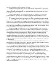
<strong>Nested</strong> designs are used when there are<br />
samples within samples. In horticulture, for<br />
example, an investigator might want to<br />
compare the transpiration rates of five<br />
Hybrid 1<br />
Pot 1 Pot 2 Pot 3<br />
OOOO OOOO OOOO OOOO OOOO OOOO<br />
Hybrid 2<br />
Pot 4 Pot 5 Pot 6<br />
OOOO OOOO OOOO OOOO OOOO OOOO<br />
Hybrid 3<br />
Pot 7 Pot 8 Pot 9<br />
OOOO OOOO OOOO OOOO OOOO OOOO<br />
Hybrid 4<br />
Pot 10 Pot 11 Pot 12<br />
OOOO OOOO OOOO OOOO OOOO OOOO<br />
Hybrid 5<br />
Pot 13 Pot 14 Pot 15<br />
OOOO OOOO OOOO OOOO OOOO OOOO<br />
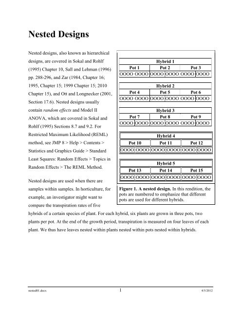
Figure 1. A nested design. In this rendition, the<br />
pots are numbered to emphasize that different<br />
pots are used for different hybrids.<br />
hybrids of a certain species of plant. For each hybrid, six plants are grown in three pots, two<br />
plants per pot. At the end of the growth period, transpiration is measured on four leaves of each<br />
plant. We thus have leaves nested within plants nested within pots nested within hybrids.<br />
nested01.docx 1 4/5/2012
1. Model<br />
or<br />
or<br />
Hybrid 1<br />
Pot 1(1) Pot 2(1) Pot 3(1)<br />
OOOO OOOO OOOO OOOO OOOO OOOO<br />
Hybrid 2<br />
Pot 1(2) Pot 2(2) Pot 3(2)<br />
OOOO OOOO OOOO OOOO OOOO OOOO<br />
Hybrid 3<br />
Pot 1(3) Pot 2(3) Pot 3(3)<br />
OOOO OOOO OOOO OOOO OOOO OOOO<br />
Hybrid 4<br />
Pot 1(4) Pot 2(4) Pot 3(4)<br />
OOOO OOOO OOOO OOOO OOOO OOOO<br />
Hybrid 5<br />
Pot 1(5) Pot 2(5) Pot 3(5)<br />
OOOO OOOO OOOO OOOO OOOO OOOO<br />
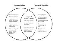
Figure 2. A nested design.<br />
Y B C e<br />
(1)<br />
, <br />
ijkl i j i k i j l ijk<br />
, <br />
Y B C B e<br />
ijkl i ij ijk ijkl<br />
nested01.docx 2 4/5/2012
Quantitative<br />
Response<br />
=<br />
Constant<br />
(grand mean) +<br />
where the quantitative response,<br />
Effects of Factor A<br />
nested01.docx 3 4/5/2012<br />
+<br />
Effects of Factor B nested within A<br />
+<br />
Effects of Factor C nested within A and B<br />
+<br />
[possible additional nested factors]<br />
+ Residual<br />
"error"<br />
Y ijkl is the transpiration rate (units unknown) on leaf l nested within plant k nested within pot j<br />
nested within hybrid i,<br />
i is the fixed effect of hybrid i , i = 1, 2, 3, 4, 5,<br />
B B is the random effect of pot j nested within hybrid i, j = 1, 2, 3,<br />
<br />
ji ij<br />
C C B is the random effect of plant k nested within hybrid i and pot j, k = 1, 2, and<br />
eijkl<br />
, , <br />
k i j ijk<br />
is the random effect of leaf l nested within hybrid i, pot j, and plant k, l = 1, 2, 3, 4.<br />
The variables that define the nested factors are categorical.<br />
The effects, moreover, can be fixed or random.<br />
Fixed effects are what we have dealt with so far in one- and two-factor Anova. With fixed<br />
effects, the levels of the factor used in the study are the specific levels we are interested in.<br />
Random effects are the effects of factor-levels that have been randomly selected as<br />
representatives of a larger population of factor-levels. Blocks are usually random.<br />
In the example above, the investigator is not interested specifically in the 15 pots that are used in<br />
the experiment, but he is interested in measuring the random variation in the response that is<br />
attributable to pots. The same can be said of the plants and leaves. The pots, the plants, and the<br />
leaves are random selected from the populations of pots, plants, and leaves. The hybrids, on the
other hand, have fixed effects. The investigator is interested in the effects of these five specific<br />
hybrids. They are not randomly selected representatives of a larger population of hybrids. Thus,<br />
their effects are fixed rather than random.<br />
Ott and Longnecker (2001, Section 17.1) have these definitions:<br />
In a fixed-effects model for an experiment, all the factors in the experiment have<br />
a predetermined set of levels and the only inferences are for the levels of the<br />
factors actually used in the experiment.<br />
In a random effects model for an experiment, the levels of factors used in the<br />
experiment are randomly selected from a population of possible levels. The<br />
inferences from the data in the experiment are for all levels of the factors in the<br />
population from which the levels were selected and not only the levels used in the<br />
experiment.<br />
In a mixed effects model for an experiment, the levels of some of the factors used<br />
in the experiment are randomly selected from a population of possible levels,<br />
whereas the levels of the other factors in the experiment are predetermined. The<br />
inferences from the data in the experiment concerning the factors with fixed levels<br />
are only for the levels if the factors used in the experiment, whereas inferences<br />
concerning factors with randomly selected levels are for all levels of the factors in<br />
the population from which the levels were selected.<br />
D e , or by<br />
Notation. It would make sense to denote the random effect of leaf l by ijkl<br />
<br />
D , B, C eijkl<br />
, or even by e eijklbecause<br />
it is a nested effect just like B and C. But the<br />
ijkl<br />
l ijk<br />
fact is that all of the error terms in Anova are always random effects, and, being replicates, are<br />
necessarily nested within other effects.<br />
It is traditional to represent fixed effects by Greek letters and random effects by English letters.<br />
nested01.docx 4 4/5/2012<br />
l ijk
Random effects are random variables, while fixed effects are constant parameters. Being<br />
random variables, random effects have a probability distribution (with mean, standard<br />
deviation, and shape). In this respect, random effects are much like additional error terms, like<br />
the residual, e.<br />
Assumptions<br />
Fixed effects are unknown constants. The fixed effects sum to zero for each factor. Thus,<br />
<br />
i<br />
0 . The effect of each hybrid i, i = 1, 2, 3, 4, 5, is<br />
i<br />
,<br />
1, 2, ..., 5<br />
i i i<br />
the amount i by which the mean transpiration rate i of hybrid i differs from the mean<br />
transpiration rate of all five hybrids <br />
. We are interested in<br />
1 2 3 4 5 5<br />
the five effects, 1, 2, , 3, 4, 5,<br />
of hybrids 1, 2, 3, 4, and 5 specifically.<br />
o We want to test hypotheses about these 5 numeric parameters. If we find there are<br />
no significant differences in transpiration rate among these five hybrids, we will<br />
have to look to other factors that might have (nonzero) effects.<br />
o If there are significant differences, we will want to estimate the effects and means<br />
of each of the 5 hybrids. We may want to know which hybrids have the highest or<br />
lowest effects, so we may want to perform multiple comparisons and test and<br />
estimate contrasts of the hybrid mean transpiration rates.<br />
Random effects are random variables, because they are the effects of randomly selected<br />
levels of the factor. The random effects of pots, for example, are the 15 random variables<br />
B , B , B ; B , B , B , , B , B , B (2)<br />
<br />
1 1 2 1 3 1 1 2 2 2 3 2 1 5 2 5 3 5<br />
They are random, because they are the 15 effects of 15 randomly selected pots. For each<br />
pot j(i), the amount B ji by which the mean transpiration rate of pot j within hybrid i<br />
nested01.docx 5 4/5/2012
differs from the mean transpiration rate i of hybrid i. But we are not interested in the 15<br />
effects (2) of these 15 randomly selected pots specifically, because they are 15 of a huge<br />
population of pots that we could have used and in which we are equally interested Indeed,<br />
we are not interest in any of the pots specifically. And the same is true for the random<br />
plants within the pots, and random leaves within the plants and pots. Rather we are<br />
interested in the distribution of the random effects and random means, because the<br />
distribution describes the entire populations, and the distributions of the random effects<br />
affect transpiration rates.<br />
The random effects of each random factor are assumed to have<br />
o (central location) mean = 0, thus,<br />
<br />
<br />
E B E C E e<br />
0<br />
j i k i, j l i, j, k<br />
o (dispersion) variance homogeneous over levels, thus<br />
ji <br />
ki , j<br />
<br />
li , j, k <br />
2<br />
Var B for all ,<br />
B i j<br />
2<br />
Var C for all , ,<br />
o (shape) normal distribution, thus<br />
C i j k<br />
2<br />
Var e for all , , ,<br />
e i j k l<br />
Bji<br />
<br />
2<br />
Normal 0, B <br />
ki , j<br />
2<br />
Normal 0, C <br />
, , <br />
2<br />
Normal 0, e <br />
C<br />
e<br />
l i j k<br />
This implies that the responses Y ijkl have the following distribution<br />
o (central location)<br />
<br />
EY <br />
ijkl i<br />
nested01.docx 6 4/5/2012
o (dispersion)<br />
<br />
Yijkl iBjiCki, j el<br />
ijk <br />
Var Var<br />
00 <br />
<br />
2 2 2 2<br />
Y B C e<br />
o (shape) normal distribution, thus<br />
2 2 2<br />
B C e<br />
2 2 2<br />
<br />
Y Normal , <br />
(4)<br />
ijkl i B C e<br />
The distribution (4) of the quantitative response, the random transpiration rates Yijkl is what we<br />
have been interested in all along. We see, in (4), that the fixed effects determine the mean<br />
responses,<br />
, 1, 2, ..., 5,<br />
(5)<br />
i i i<br />
while the random effects determine the (homogeneous) variance (and standard deviation) of the<br />
responses, defined in equation (3):<br />
<br />
(6)<br />
2 2 2 2<br />
Y B C e<br />
Thus, the parameters of interest in the model are<br />
i. the means shown in equation (5) of the nonrandom factor levels, the 5 hybrids,<br />
2 2 2 2<br />
ii. the homogeneous variance of the response, <br />
Y B C e<br />
2 2 2<br />
iii. and the components of the variance of the response, , , , generally termed as the<br />
variance components.<br />
B C e<br />
To understand the response, transpiration rate, we need to make inferences about these<br />
parameters.<br />
nested01.docx 7 4/5/2012<br />
(3)
2. Hypotheses<br />
A null and alternative hypothesis can be tested for each factor in the model, random or fixed.<br />
For fixed effects, like the effects of hybrids in the above example, we would have<br />
Fixed effects, of Hybrids<br />
e.g.,<br />
H0: The effects of all hybrids = 0, versus HA: The effects of some hybrids ≠ 0,<br />
H0: i 0for<br />
all i, versus HA: i 0for<br />
some i (7)<br />
and we would state the conclusion in the usual way:<br />
or<br />
There is/is not significant statistical evidence that hybrid affects<br />
transpiration rate (P=__ ),<br />
There is/is not significant statistical evidence that mean transpiration rate<br />
differs among hybrids (P=__ ).<br />
Random Effects, of Plants for Example<br />
For random effects, like the effects of plants in the above example, we would test hypotheses<br />
about the variance components of the random factors<br />
H0: The standard deviation of the random effects of plants = 0,<br />
versus<br />
HA: The standard deviation of the random effects of some plants ≠ 0.<br />
nested01.docx 8 4/5/2012
Symbolically,<br />
H0: σplants = 0, versus HA: σplants ≠ 0<br />
or, in terms of the model (1),<br />
2<br />
2<br />
H0: 0,<br />
versus HA: 0<br />
(8)<br />
C<br />
and we would state the conclusion in the usual way:<br />
or<br />
C<br />
There is/is not significant statistical evidence that variance among plants is a<br />
component in the variation of transpiration rate (P=__ ),<br />
There is/is not significant statistical evidence that transpiration rate varies<br />
among plants (P=__ ).<br />
Random Effects of Pots<br />
We would analyze the variance component due to pots in the same way, i.e., we would test the<br />
hypothesis<br />
2<br />
2<br />
H0: 0 , versus HA: 0<br />
(9)<br />
B<br />
B<br />
If a variance component, e.g., the variance of the random effects of pots or of plants in this case,<br />
is statistically significant, then we want to estimate it. This is best done using statistical software.<br />
nested01.docx 9 4/5/2012
3. F-Tests<br />
F = MSA/MSB tests the null hypothesis that the mean transpiration rate is the same for all five<br />
hybrids versus the alternative that the mean transpiration rate is different for some hybrids.<br />
Alternatively, this could be stated as: F = MSA/MSB tests the null hypothesis (7) that the effects<br />
of all of the hybrids on mean transpiration rate are zero, versus the alternative that the effects of<br />
some of the hybrids are non-zero.<br />
F = MSB/MSC test the null hypothesis that there is no variation in mean transpiration rate<br />
among pots within each hybrid, versus the alternative that there is some variation among pots<br />
within some hybrids:<br />
2<br />
2<br />
H0: 0 , versus HA: 0<br />
(9)<br />
B<br />
B<br />
Finally, F = MSC/MSE tests the null hypothesis that there is no variation in mean transpiration<br />
rate among plants within each pot, versus the alternative that there is some variation among<br />
plants within some pots:<br />
2<br />
2<br />
H0: 0,<br />
versus HA: 0<br />
(8)<br />
C<br />
C<br />
As explained above, the latter two sets of hypotheses are stated in terms of "variation" rather than<br />
in terms of "means" or of "effects" because the effects of pots and plants are assumed to be<br />
random variables rather than fixed constants. Since the effects are random, we cannot assume<br />
they sum to zero as we would if they were fixed. Therefore it would be meaningless to test the<br />
hypothesis that all the random effects are zero. On the other hand, the assumption that the effects<br />
are random variables does make it reasonable to test the hypothesis that the variance of those<br />
random variables is zero, and that is what we are doing. An effect is random rather than fixed<br />
when the levels tested are a random sample from the set of all levels of interest.<br />
nested01.docx 10 4/5/2012
4. Design<br />
Significance level 0.05<br />
a = 5 hybrids (i.e., levels of Factor A)<br />
b = n1 n2 n3 n4 n5<br />
3pots<br />
(i.e., levels of Factor B) within each hybrid requiring 5×3 = 15<br />
pots in all.<br />
n n n plants (i.e., levels of Factor C) within each pot and hybrid requiring<br />
c = 2 = 11 21 23 3×2 = 6 plants of each hybrid, and 5×3×2 = 30 plants in all.<br />
n n n leaves (i.e., levels of Factor D) within each plant, pot and hybrid<br />
d = 4 = 11,1 21,1 25,3 <br />
requiring 4 leaves randomly selected from each plant of each hybrid, and 5×3×2×4 =<br />
120 leaves in all.<br />
We choose the number of levels if the fixed factor(s)—here, hybrids—according to the number<br />
that are of interest.<br />
We choose the number of levels of random factor(s) )—here, pots, plants, and leaves—according<br />
to their influence on power of the F-tests and precisions of the estimators. The power and the<br />
precision depend on the degrees of freedom of the sources of variation, which we consider at the<br />
design stage of the experiment.<br />
nested01.docx 11 4/5/2012
Degrees of Freedom<br />
Source df<br />
5 Hybrid 5 - 1 = 4<br />
3 Pot (Hybrid) 5 x (3 - 1) = 10<br />
2 Plant (Pot Hybrid) 5 x 3 x (2 - 1) = 15<br />
Model 29<br />
4 Error = Leaves (Plant Pot Hybrid) 5 x 3 x 2 x (4 - 1) = 90<br />
Total (5 x 3 x 2 x 4) - 1 = 119<br />
The power of the various F-tests can be traced to the degrees of freedom by means of the Anova<br />
table.<br />
Anova<br />
Source df SS MS F<br />
Hybrid 4 SSA MSA = SSA/4 F = MSA/MSB<br />
Pot (Hybrid) 10 SSB MSB = SSB/10 F = MSB/MSC<br />
Plant (Pot Hybrid) 15 SSC MSC = SSC/15 F = MSC/MSE<br />
Model 29 SSM MSM = SSM/29<br />
Error 90 SSE MSE = SSE/90<br />
Total 119<br />
nested01.docx 12 4/5/2012
Alternative Allocation of Experimental Units<br />
A benefit of careful design of experiments is the ability to consider alternative designs, and<br />
alternative allocation of experimental units within designs.<br />
In the present example, the consequences of two alternatives might be considered.<br />
The first alternative would be simply to assay one less leaf per plant. The second alternative<br />
would be to assay one less leaf per plant, but one more pot per hybrid.<br />
Original Design Alternative 1 Alternative 2<br />
Source Levels Units df Levels Units df Levels Units df<br />
Hybrid 5 5 4 5 5 4 5 5 4<br />
Pot 3 15 10 3 15 10 4 20 15<br />
Plant 2 30 15 2 30 15 2 40 20<br />
Leaves 4 120 90 3 90 60 3 120 80<br />
Total 119 89 119<br />
5. Gather Data and Compute<br />
JMP Implementation<br />
In JMP, select Analyze, Fit Model, and proceed as explained in Sall and Lehman (2001, pp. 330-<br />
337). For much more information and detail see JMP, Help, Statistics Guide, Standard Least<br />
Squares, Topics in Random Effects and Specifying Random Effects.<br />
nested01.docx 13 4/5/2012
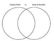
To declare random effects in JMP, select " Attributes:" in the Fit-Model Dialog (shown above),<br />
as shown in Figure 12.21 on p. 235 of Sall, Lehman, and Creighton 2001.<br />
F-Tests in JMP<br />
In JMP, the proper tests are obtained by the method explained on p. 330-336 of Sall, Lehman and<br />
Creighton 2001. Note that the correct explained under Method 1: Random Effects-Mixed<br />
Model, pp. 333-336.<br />
nested01.docx 14 4/5/2012
Estimating Variance Components in JMP<br />
As mentioned earlier, if there is statistically significant variation in the response due to random<br />
effects, then we usually want to estimate the variance component, and see what portion is due to<br />
each random factor. In JMP, using the Traditional Expected Mean Square (EMS) method of<br />
analysis in the FIT MODEL platform, the variance components are estimated automatically. See<br />
JMP, Help, Statistics Guide, Standard Least Squares, Specifying Random Effects, Method<br />
of Moments Results.<br />
See file <strong>Nested</strong>Transpiration.JMP (…data/Examples/<strong>Nested</strong>Transpiration.JMP)<br />
JMP Output using Fit Model with Traditional EMS Method<br />
Response Transpiration Rate<br />
Summary of Fit<br />
RSquare 0.968927<br />
RSquare Adj 0.958914<br />
Root Mean Square Error 0.923135<br />
Mean of Response 51.43619<br />
Observations (or Sum Wgts) 120<br />
Analysis of Variance<br />
Source DF Sum of Squares Mean Square F Ratio<br />
Model 29 2391.5257 82.4664 96.7712<br />
Error 90 76.6961 0.8522 Prob > F<br />
C. Total 119 2468.2218
Tests wrt Random Effects<br />
Source SS MS Num DF Num F Ratio Prob > F<br />
Hybrid 2275.96 568.99 4 69.9579
Least Squares Means Table<br />
Level Least Sq Mean Std Error Mean<br />
1 45.524375 0.58214105 45.5244<br />
2 48.150857 0.58214105 48.1509<br />
3 51.296105 0.58214105 51.2961<br />
4 54.449997 0.58214105 54.4500<br />
5 57.759636 0.58214105 57.7596<br />
LSMeans Differences Tukey HSD<br />
α=0.050 Q=3.29108<br />
Level Least Sq Mean<br />
5 A 57.759636<br />
4 B 54.449997<br />
3 C 51.296105<br />
2 D 48.150857<br />
1 D 45.524375<br />
Levels not connected by same letter are significantly different.<br />
This output becomes Table 2 in the results section of the conclusion.<br />
SAS Implementation<br />
The SAS model statement in PROC ANOVA or PROC GLM would be<br />
MODEL TRANSPIR = HYBRID POT(HYBRID) PLANT(POT HYBRID);<br />
F-Tests in SAS<br />
The SAS Statements:<br />
PROC ANOVA; CLASS HYBRID POT PLANT;<br />
MODEL TRANSPIR = HYBRID POT(HYBRID) PLANT(POT HYBRID);<br />
will perform only the third of the three desired F-tests automatically. The first two hypotheses,<br />
whose F-tests do not have MSE in the denominator, will not be performed automatically. This is<br />
because SAS automatically uses the mean squared error (MSE) as the denominator for all F-<br />
tests, so that the F values that SAS produces for the first and second tests are incorrect.<br />
There are two ways to get the correct values.<br />
nested01.docx 17 4/5/2012
The first way is to use the sums of squares and degrees of freedom computed by SAS to calculate<br />
"by hand" the mean squares and the proper Fs.<br />
The second way is use a TEST statement with PROC ANOVA or with PROC GLM. The TEST<br />
statement syntax is<br />
TEST H=numerator mean square E=denominator mean square;<br />
where "numerator mean square" represents the factor in the model statement whose mean square<br />
goes in the numerator, and where "denominator mean square" represents the factor in the model<br />
statement whose mean square goes in the denominator. Another way to think of it is that "H"<br />
stands for "Hypothesis" and "E" stands for "Error". "H=" signifies the factor about which we<br />
wish to test a hypothesis, and "E=" signifies the factor we wish to use as an error term for the<br />
test.<br />
To test the first two hypotheses mentioned earlier we would use the following TEST statements.<br />
TEST H=HYBRID E=POTS(HYBRID);<br />
TEST H=POTS(HYBRID) E=PLANT(POTS HYBRID);<br />
6. Conclusion<br />
As always, the conclusion is a statement about the alternative hypothesis.<br />
For fixed effects, the hypotheses are about unknown constant parameters, and the conclusion, as<br />
mentioned above, would take the form<br />
or<br />
There is/is not significant statistical evidence that hybrid affects<br />
transpiration rate (P=__ ),<br />
There is/is not significant statistical evidence that mean transpiration rate<br />
differes among hybrids (P=__ ).<br />
nested01.docx 18 4/5/2012
For random effects, the hypotheses are about variance components, the variance (or standard<br />
deviation) of the random variable whose categories define the random effects, and, as mentioned<br />
earlier, the conclusion would take the form<br />
Or<br />
There is/is not significant statistical evidence that variance among plants is a<br />
component in the variation of transpiration rate (P=__ ),<br />
There is/is not significant statistical evidence that transpiration rate varies among<br />
plants (P=__ ).<br />
For the transpiration example we would conclude as follows.<br />
Report<br />
There is significant statistical evidence that the mean transpiration rate (units) varies across<br />
hybrids (1, 2, 3, 4, 5), as shown in Table 2 (P < 0.001).<br />
Table 2. Mean transpiration rate by hybrid (1, 2, 3, 4, 5)<br />
Hybrid n Mean* SE<br />
95% Confidence<br />
Interval<br />
5 3 57.8 a 0.582 (56.5, 59.1)<br />
4 3 54.4 b 0.582 (53.2, 55.7)<br />
3 3 51.3 c 0.582 (50.0, 52.6)<br />
2 3 48.2 d 0.582 (46.9, 49.4)<br />
1 3 45.5 d 0.582 (44.2, 46.8)<br />
*Means followed by the same superscript are not<br />
significantly different at the 0.05 level<br />
experiment wise using the Kramer-Tukey HSD<br />
(Zar 1999) .<br />
nested01.docx 19 4/5/2012
The variance components due to pots within hybrids and plots within hybrids and pots are<br />
statistically significant but not important, as shown in .<br />
Table 3 Variance components of transpiration rate. The pots- and plants-components are<br />
statistically significant but not important, because they are both smaller than the<br />
residual error variation of leaves, as shown by the ratios being less than 1.<br />
Source<br />
Variance<br />
Component Percent P Ratio<br />
Pots(Hybrid) 0.73 37.7 0.013 0.86<br />
Plant(Hybrid,Pots) 0.36 18.4 0.002 0.42<br />
Error=Leaves(Hy,Pots,Pl) 0.85 43.9 1.00<br />
Total 1.94 100.0<br />
Example 16.1, p. 254 Zar (1984) = 15.1, p. 304 Zar (1995)<br />
Zar (1984, p. 253; 1995 p. 303) does a good job of explaining the difference between "crossed"<br />
and "nested". He then introduces an example wherein the effects of three different drugs on<br />
cholesterol concentration are investigated. He explains that samples of each of the drugs were<br />
obtained from two sources, and no two different drugs were obtained from the same source, i.e.,<br />
there are six distinct sources. Hence, the sources are nested within drugs rather than crossed with<br />
drugs.<br />
Zar doesn't specify the nature of the sources, except to mention that they are random. It would<br />
make sense, for example, if the six sources--A, Q, D, B, L, and S--are six different pharmacies or<br />
pharmacists.<br />
1. Describe circumstances under which the sources would be crossed with drugs, rather than<br />
nested within drugs.<br />
2. If the various manufacturers were randomly selected from a population of manufacturers,<br />
then it makes sense to assume that the effects of sources are random. Describe<br />
circumstances under which the sources would be fixed rather than random.<br />
nested01.docx 20 4/5/2012
Methods<br />
The effects on mean human female blood cholesterol concentration (mg/100 ml plasma) of three<br />
drugs (1, 2, and 3), each drug obtained from two of six randomly selected sources (A, Q, D, B, L,<br />
and S), was studied by analysis of variance of a balanced, nested design. Drug 1 was obtained<br />
from sources A and Q, Drug 2 was obtained from sources D and B, and Drug 3 was obtained<br />
from sources L and S. Two determinations of cholesterol concentration was made from each<br />
drug from each source, so four determinations were made for each drug, and twelve<br />
determinations were made in all.<br />
[Although it is obviously an important point, Zar doesn't tell us anything about the human female<br />
subjects! It could be that each drug from each source was given to one female (i.e., six females in<br />
all), and then two blood samples from each female comprise the two determinations. But I<br />
believe it would be better if (and therefore we shall pretend that)]<br />
Each drug from each source was administered to two randomly selected human females (12<br />
females in all), and serum cholesterol concentration was determined using a well known assay<br />
procedure.<br />
In summary, three drugs were compared, with two sources nested within each drug, and with two<br />
determinations nested within each source.<br />
Drug 1 Drug 2 Drug 3<br />
Source A Source Q Source D Source B Source L Source S<br />
Female 1 Female 3 Female 5 Female 7 Female 9 Female 11<br />
Female 2 Female 4 Female 6 Female 8 Female 10 Female 12<br />
1. What, specifically, would be wrong with the design if each drug from each source had<br />
been given to one female (i.e., six females in all), and if two blood samples drawn from<br />
each female were then used as the two determinations?<br />
nested01.docx 21 4/5/2012
Computations<br />
SAS<br />
TITLE1 'NESTED01 SAS: Example 16.1, p. 254, Zar (1974)';<br />
DATA ONE; INPUT DRUG SOURCE $ CHOLEST; LIST; CARDS;<br />
1 A 102<br />
1 A 104<br />
1 Q 103<br />
1 Q 104<br />
2 D 108<br />
2 D 110<br />
2 B 109<br />
2 B 108<br />
3 L 104<br />
3 L 106<br />
3 S 105<br />
3 S 107<br />
;<br />
PROC ANOVA; CLASS DRUG SOURCE; MODEL CHOLEST = DRUG SOURCE(DRUG);<br />
TEST H=DRUG E=SOURCE(DRUG); MEANS DRUG / TUKEY E=SOURCE(DRUG);<br />
MEANS DRUG / TUKEY ;<br />
JMP<br />
The results of JMP Analyze, Fit Model, Choltesterol = Drug Source(Drug){Random}. The<br />
data are in file <strong>Nested</strong>DrugEG.jmp. and file <strong>Nested</strong>DrugEG.MTW.<br />
nested01.docx 22 4/5/2012
ANOVA Table<br />
ANOVA<br />
---------------------------------------------------------------------<br />
Source df SS MS F P R 2<br />
---------------------------------------------------------------------<br />
Drug 2 61.17 30.58 61.17 .004 85%<br />
Source(Drug) 3 1.50 0.50 0.33 >.80 2%<br />
---------------------------------------------------------------------<br />
Model 5 62.67 12.53 87%<br />
Residual 6 9.00 1.50 13%<br />
---------------------------------------------------------------------<br />
Total 11 71.67 100%<br />
Note. Two different MEANS statements have been used to get the results of Tukey's HSD test.<br />
The first statement, which, which uses the E= option, correctly asks that the standard error be<br />
estimated by<br />
sqrt(MSSource(Drug) / n) = sqrt(0.50 / 4) = 0.354.<br />
The second MEANS statement, by not specifying an error mean square, erroneously allows the<br />
standard error to be estimated by<br />
sqrt(MSResidual / n) = sqrt(1.50 / 4) = 0.612.<br />
The choice of the "error term" (i.e., denominator of the F statistic) makes an important difference<br />
in this example.<br />
Note. In this example, the "Residual" variation, i.e., the source of variation that SAS calls<br />
"ERROR", includes (i) variation among the female subjects (within source and drug), and (ii)<br />
experimental error. Hence, in this example, the name "residual" might be a little more accurate<br />
than "error" or "unexplained". On the other hand, many statisticians, e.g., Snedecor and Cochran,<br />
would call this source of variation "Subjects within Source and Drug" or "Females within Source<br />
and Drug".<br />
nested01.docx 23 4/5/2012
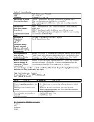
Results<br />
There were significant<br />
differences among drugs in the<br />
mean cholesterol concentration<br />
(mg/100 ml plasma) of human<br />
females (P = .004), and no<br />
significant differences among<br />
sources (P > .50). Eighty five<br />
percent of the variation in<br />
cholesterol concentration was<br />
explained by differences among drugs, only 2 percent was attributable to variation among<br />
sources, and 13% was unexplained. See Table 1.<br />
Pig Breeding Exercise (Snedecor and Cochran, 6th edition, pp. 288-289)<br />
For an evaluation of the breeding value of sires in pig-<br />
raising, each sire is mated to a random group of dams,<br />
each mating producing a litter of pigs whose<br />
characteristics are the criteria. The data below were<br />
obtained by randomly selecting two pigs from each litter<br />
and using the average daily weight gain (g) of the pigs as<br />
the criterion for evaluation.<br />
1) Verbally state the hypotheses that can be tested by<br />
ANOVA. Be careful about distinguishing between<br />
fixed and random effects, and justify your decision to<br />
used fixed or random effects.<br />
2) Write a "methods" paragraph for this experiment.<br />
3) Use JMP to analyze the data, but do not hand in any computer output.<br />
a) Analyze using the traditional EMS method,<br />
i) and transcribe the relevant information into an ANOVA table, including partial R 2 ,<br />
and hand in that table.<br />
Table 1. Mean human female cholesterol<br />
concentration after drug treatment.<br />
---------------------------------------------<br />
Mean Conc * Std. Error<br />
Drug n (mg/100 ml) (mg/100 ml)<br />
---------------------------------------------<br />
Drug 2 4 108.8 a 0.354<br />
Drug 3 4 105.5 b 0.354<br />
Drug 1 4 103.3 c 0.354<br />
---------------------------------------------<br />
* Means followed by the same letter are not<br />
significantly different at the .05 level<br />
(experimentwise), using Tukey's HSD (Zar,<br />
1984, pp. 186-190, 259).<br />
Sire Dam Pig Gains<br />
-------------------------<br />
1 1 2.77 2.38<br />
2 2.58 2.94<br />
-------------------------<br />
2 1 2.28 2.22<br />
2 3.01 2.61<br />
-------------------------<br />
3 1 2.36 2.71<br />
2 2.72 2.74<br />
-------------------------<br />
4 1 2.87 2.46<br />
2 2.31 2.24<br />
-------------------------<br />
5 1 2.74 2.56<br />
2 2.50 2.48<br />
-------------------------<br />
nested01.docx 24 4/5/2012
ii) Write a "results" paragraph. Don't bother with post hoc analyses.<br />
b) Analyze using the recommended REML method,<br />
i) and write a results paragraph (an Anova table is not relevant using REML).<br />
ii) In the results paragraph, include results of the test involving sires and the test<br />
involving dams nested within sires.<br />
iii) In the results paragraph, for fixed effects, site the F ratio with its numerator and<br />
denominator degrees of freedom, and the P-value, parenthetically, e.g., (F3,6 = 5.6, P<br />
= 0.004).<br />
iv) In the results paragraph, for random effects, site the point estimate of the variance<br />
component, its ratio to the residual variance, its percent of the total variance, and its<br />
95% confidence interval.<br />
v) Interpret this in terms of statistical significance and practical importance.<br />
c) Do EMS and REML agree?<br />
© 1997-2012, Golde I. Holtzman, all rights reserved<br />
Send Suggestions or Comments to Golde I. Holtzman<br />
Department of Statistics<br />
URL: …/STAT5606/nested01.docx<br />
Last updated: April 5, 2012<br />
nested01.docx 25 4/5/2012