iCoseg: Interactive Co-segmentation with Intelligent Scribble Guidance

iCoseg: Interactive Co-segmentation with Intelligent Scribble Guidance
Dhruv Batra
Carnegie Mellon Univerity
www.ece.cmu.edu/˜dbatra
Jiebo Luo
Eastman Kodak Company
jiebo.luo@kodak.com
Adarsh Kowdle
Cornell University
apk64@cornell.edu
Devi Parikh
Toyota Technological Institute at Chicago (TTIC)
Tsuhan Chen
Cornell University
tsuhan@ece.cornell.edu
dparikh@ttic.edu
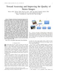
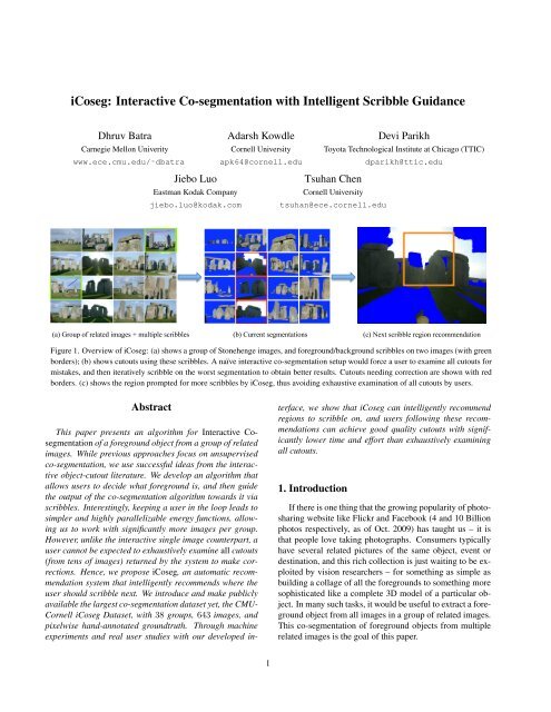
(a) Group of related images + multiple scribbles (b) Current segmentations (c) Next scribble region recommendation
Figure 1. Overview of iCoseg: (a) shows a group of Stonehenge images, and foreground/background scribbles on two images (with green
borders); (b) shows cutouts using these scribbles. A naïve interactive co-segmentation setup would force a user to examine all cutouts for
mistakes, and then iteratively scribble on the worst segmentation to obtain better results. Cutouts needing correction are shown with red
borders. (c) shows the region prompted for more scribbles by iCoseg, thus avoiding exhaustive examination of all cutouts by users.
Abstract
This paper presents an algorithm for Interactive Cosegmentation
of a foreground object from a group of related
images. While previous approaches focus on unsupervised
co-segmentation, we use successful ideas from the interactive
object-cutout literature. We develop an algorithm that
allows users to decide what foreground is, and then guide
the output of the co-segmentation algorithm towards it via
scribbles. Interestingly, keeping a user in the loop leads to
simpler and highly parallelizable energy functions, allowing
us to work with significantly more images per group.
However, unlike the interactive single image counterpart, a
user cannot be expected to exhaustively examine all cutouts
(from tens of images) returned by the system to make corrections.
Hence, we propose iCoseg, an automatic recommendation
system that intelligently recommends where the
user should scribble next. We introduce and make publicly
available the largest co-segmentation dataset yet, the CMU-
Cornell iCoseg Dataset, with 38 groups, 643 images, and
pixelwise hand-annotated groundtruth. Through machine
experiments and real user studies with our developed in-
1
terface, we show that iCoseg can intelligently recommend
regions to scribble on, and users following these recommendations
can achieve good quality cutouts with significantly
lower time and effort than exhaustively examining
all cutouts.
1. Introduction
If there is one thing that the growing popularity of photosharing
website like Flickr and Facebook (4 and 10 Billion
photos respectively, as of Oct. 2009) has taught us – it is
that people love taking photographs. Consumers typically
have several related pictures of the same object, event or
destination, and this rich collection is just waiting to be exploited
by vision researchers – for something as simple as
building a collage of all the foregrounds to something more
sophisticated like a complete 3D model of a particular object.
In many such tasks, it would be useful to extract a foreground
object from all images in a group of related images.
This co-segmentation of foreground objects from multiple
related images is the goal of this paper.

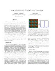
(a) Stone-pair [23]. (b) Stonehenge-pair from CMU-Cornell iCoseg Dataset.
Figure 2: What is foreground? The stone-pair (a) has significant variation in background with nearly identical foreground and thus
unsupervised co-segmentation can easily extract the stone as foreground. The Stonehenge-pair is fairly consistent as a whole and thus
the stones cannot be cut out via unsupervised co-segmentation. Bringing a user in the loop is necessary for the problem of foreground
extraction to be well defined.
Most existing works on co-segmentation [13, 21, 23]
work with a pair of images with similar (sometimes nearly
identical) foreground, and unrelated backgrounds (e.g. the
“Stone-pair” in Figure 2). This property is necessary because
the goal of these works is to extract the common foreground
object automatically, without any user-input. Due
to the nature of our application (i.e. multiple images of the
same event or subject), our images typically do not follow
this property (see Figure 2). Hence, without user-input, the
task of extracting the foreground object “of interest” is illdefined.
This paper deals with Interactive Co-segmentation of a
group (typically ≫ 2) of related images, and presents an
algorithm that enables users to quickly guide the output of
the co-segmentation algorithm towards the desired output
via scribbles. Our approach uses successful ideas from the
single-image interactive segmentation [6, 19, 22] literature.
A user provides foreground/background scribbles on one
(or more) images from a group and our algorithm uses these
scribbles to produce cutouts from all images this group.
In a single-image setup, a user visually inspects the produced
cutout and gives more scribbles to correct mistakes
made by the algorithm. However, this approach would not
work for interactive co-segmentation because 1) as the number
of images in the group increases, it becomes increasingly
cumbersome for a user to iterate through all the images
in the group to find the worst segmentation; and 2) even
if the user were willing to identify an incorrect cutout, there
might be multiple incorrect cutouts in the group, some more
confusing to the segmentation algorithm than others. Observing
labels on the most confusing ones first would help
reduce the number of user annotations required. It is thus
necessary for the algorithm to be able to suggest regions in
images where scribbles would be the most informative.
Contributions. The main contributions of this paper are:
• We present the first algorithm for intelligent Interactive
Co-segmentation (iCoseg), that automatically suggests
regions where the user should scribble next.
• We introduce (and show results on) the largest cosegmentation
dataset yet, the CMU-Cornell iCoseg
dataset, containing 38 groups with 17 images/group
on average (total 643 images) and pixelwise handannotated
groundtruth. We make this dataset (and annotations)
publicly available [3] to facilitate further
work, and allow for easy comparisons.
• We develop a publicly available interface [3] for interactive
co-sgementation. We present results of simulated
machine experiments as well as real user studies
on our interface. We find that iCoseg can intelligently
recommend regions to scribble on, and help users
achieve good quality cutouts with significantly lower
time and effort than having to examine all cutouts exhaustively.
Technique. Our approach is composed of two main parts:
1) an energy minimization framework for interactive cosegmentation;
and 2) a scribble guidance system that uses
active learning and some intuitive cues to form a recommendation
map for each image in the group. The system recommends
a region with the highest recommendation score. See
Figure 1 for an overview.
Organization. The rest of this paper is organized as
follows: Section 2 discusses related work; Section 3
presents our energy minimization approach to interactive
co-segmentation of a group of related images; Section 4
presents our recommendation scheme for guiding user
scribbles; Section 5 introduces our benchmark dataset; Section
6 discusses the results of simulated machine experiments
and a real user-study; Finally, Section 7 concludes
the paper.
2. Related Work
Unsupervised Co-segmentation. Rother et al. [23] introduced
the problem of (unsupervised) co-segmentation

of image pairs. Their approach is to minimize an energy
function that is a combination of the usual MRF
smoothness prior and a histogram matching term that forces
foreground histograms of images to be similar. Mu et
al. [20] extend this framework with quadratic global constraints.
More recently, Mukherjee et al. [21] proposed
half-integrality algorithms, and Hochbaum et al. [13] modified
the histogram matching term to propose max-flow
based algorithms. The common theme here is unsupervised
co-segmentation, which is achieved by forcing histogram
consistency between foregrounds. As noted earlier,
this would fail for pairs with related backgrounds (see
Figure 2), where the problem of identifying the foreground
objects is ill-posed. This is where our work of interactive
co-segmentation fits in, which allows a user to indicate the
foreground objects through simple scribbles. In addition,
these works involve specific constructions and solutions for
image pairs, while our technique naturally generalizes to
multiple images (Section 3).
Supervised Co-segmentation. Schnitman et al. [24] and
Cui et al. [12] learn to segment from a single fully segmented
image, and then “induce” [24] or “transduce” [12]
segmentations on a group of related images. We, on the
other hand, utilize very sparse user interaction (in the form
of scribles), which are not restricted to a single image and
can be provided on multiple images in a group if desired.
Interactive Image Segmentation. Boykov and Jolly [6]
posed interactive single-image segmentation given user
scribbles as a discrete optimization problem. Li et al. [19]
and Rother et al. [22] presented simplified user interactions.
Bai et al. [2] and Criminisi et al. [11] proposed techniques
built on efficient geodesic distance computations. Our approach
to multiple-image interactive co-segmentation, as
described in the next section, is a natural extension of
Boykov and Jolly [6].
Active Learning. Related to our paper are works on active
learning where algorithms are able to choose the data
they learn from by querying the labelling oracle. This is a
vast sub-field of machine learning and we refer the reader to
Settles [25] for a detailed survey. In computer vision, active
learning has been used for object categorization [15], classifying
videos [28], ranking images by informativeness [27]
and creating large datasets [9]. More recently, Kolhi et
al. [16] showed how to measure uncertainties from graphcut
solutions and suggested that these may be helpful in interactive
image segmentation applications. To the best of
our knowledge, this is the first paper to use uncertainties to
guide user scribbles.
3. iCoseg: Energy Minimization
Energy Minimization. Given user scribbles indicating
foreground / background, we cast our labelling problem
as minimization of Gibbs energies defined over
graphs constructed over each image in a group. Specifically,
consider a group of m image-scribble pairs D =
{(X (1) , S (1) ), (X (2) , S (2) ), . . . , (X (m) , S (m) )}, where the
k th image is represented as a collection of nk sites to be
labelled, i.e. X (k) = {X (k)
1
, X(k)
2
, . . . , X(k)
nk }, and scrib-
bles for an image S (k) are represented as the partial (potentially
empty) 1 set of labels for these sites. For computational
efficiency, we use superpixels as these labelling sites
(instead of pixels). 2 For each image (k), we build a graph,
G (k) = (V (k) , E (k) ), over superpixels, with edges connecting
adjacent superpixels.
Using these labelled sites, we learn a group appearance
model A = {A1, A2}, where A1 is the first-order (unary)
appearance model, and A2 the second-order (pairwise) appearance
model. This appearance model (A) is described
in detail in the following sections. We note that all images
in the group share a common model, i.e. only one model is
learnt. Using this appearance model, we define a collection
of energies over each of the m images as follows:
E (k) (X (k) : A) =
+ λ
i∈V (k)
(i,j)∈E (k)
Ei(X (k)
i
Eij
: A1)
X (k)
i , X (k)
j : A2 , (1)
where the first term is the data term indicating the cost of assigning
a superpixel to foreground and background classes,
while the second term is the smoothness term used for penalizing
label disagreement between neighbours. Note that
the (:) part in these terms indicates that both these terms are
functions of the learnt appearance model. From now on,
to simplify notation, we write these terms as Ei(Xi) and
Eij(Xi, Xj), and the dependence on the appearance model
A and image (k) is implicit.
Data (Unary) Term. Our unary appearance model consists
of a foreground and background Gaussian Mixture Model,
i.e., A1 = {GMMf , GMMb}. Specifically, we extract
colour features extracted from superpixels (as proposed by
Hoiem et al. [14]). We use features from labelled sites in
all images to fit foreground and background GMMs (where
number of gaussians was automatically learnt by minimizing
an MDL criteria [5]). We then use these learnt GMMs
to compute the data terms for all sites, which is the negative
log-likelihood of the features given the class model.
Smoothness (Pairwise) Term. The most commonly used
smoothness term in energy minimization based segmentation
methods [11, 12, 22] is the contrast sensitive Potts
model:
E(Xi, Xj) = I (Xi = Xj) exp(−βdij), (2)
1 Specifically, we require at least one labelled foreground and background
site to train our models, but only one per group, not per image.
2 We use mean-shift [10] to extract these superpixels, and typically
break down 350×500 images into 400 superpixels per image.

where I (·) is an indicator function that is 1(0) if the input
argument is true(false), dij is the distance between features
at superpixels i and j and β is a scale parameter. Intuitively,
this smoothness term tries to penalize label discontinuities
among neighbouring sites but modulates the penalty via a
contrast-sensitive term. Thus, if two adjacent superpixels
are far apart in the feature space, there would be a smaller
cost for assigning them different labels than if they were
close. However, as various authors have noted, this contrast
sensitive modulation forces the segmentation to follow
strong edges in the image, which might not necessarily correspond
to object boundaries. For example, Cui et al. [12]
modulate the distance dij based on statistics of edge profile
features learnt from a fully segmented training image.
In this work, we use a distance metric learning algorithm
to learn these dij from user scribbles. The basic intuition
is that when two features (which might be far apart in Euclidean
distance) are both labelled as the same class by the
user scribbles, we want the distance between them to be
low. Similarly, when two features are labelled as different
classes, we want the distance between them to be large, even
if they happen to be close by in Euclidean space. Thus, this
new distance metric captures the pairwise statistics of the
data better than Euclidean distance. For example, if colours
blue and white were both scribbled as foreground, then the
new distance metric would learn a small distance between
them, and thus, a blue-white edge in the image would be
heavily penalized for label discontinuity, while the standard
contrast sensitive model would not penalize this edge as
much. The specific choice of this algorithms is not important,
and any state-of-art technique may be used. We use the
implementation of Batra et al. [4].
We update both A1 = {GMMf , GMMb} and A2 =
{dij} every time the user provides a new scribble. Finally,
we note that contrast-sensitive potts model leads to a submodular
energy function. We use graph-cuts to efficiently
compute the MAP labels for all images, using the implementation
of Bagon [1] and Boykov et al. [7, 8, 17].
Comparing Energy Functions. Our introduced energy
functions (1) are different from those typically found in cosegmentation
literature and we make the following observations.
While previous works [13, 20, 21, 23] have formulated
co-segmentation of image pairs with a single energy
function, we assign to each image its own energy function.
The reason we are able to do this is because we model the
dependance between images implicitly via the common appearance
model (A), while previous works added an explicit
histogram matching term to the common energy function.
There are two distinct advantages of our approach. First, as
several authors [13, 20, 21, 23] have pointed out, adding an
explicit histogram matching term makes the energy function
intractable. On the other hand, each one of our energy functions
is submodular and can be solved with a single graph-
cut. Second, this common energy function grows at least
quadratically with the number of images in the group, making
these approaches almost impossible to scale to dozens of
images in a group. On the other hand, given the appearance
models, our collection of energy functions are completely
independent. Thus the size of our problem only grows linearly
in the number of images in the group, which is critical
for interactive applications. In fact, each one of our energy
functions may be optimized in parallel, making our
approach amenable to distributed systems and multi-core
architectures. Videos embedded on our project website [3]
show our (single-core) implementation co-segmenting ∼ 20
image in a matter of seconds.
To be fair, we should note that what allows us to set-up an
efficiently solvable energy function is our incorporation of
a user in the co-segmentation process, giving us partially labelled
data (scribbles). While this user involvement is necessary
because we work with globally related images, this
involvement also means that the co-segmentation algorithm
must be able to query/guide user scribbles, because users
cannot be expected to examine all cutouts at each iteration.
This is described next.
4. iCoseg: Guiding User Scribbles
In this section, we develop an intelligent recommendation
algorithm to automatically seek user-scribbles and reduce
the user effort. Given a set of initial scribbles from the
user, we compute a recommendation map for each image
in the group. The image (and region) with the highest recommendation
score is presented to the user to receive more
scribbles. Instead of committing to a single confusion measure
as our recommendation score, which might be noisy,
we use a number of “cues”. These cues are then combined
to form a final recommendation map, as seen in Figure 3.
The three categories of cues we use, and our approach to
learning the weights of the combination are described next.
4.1. Uncertainty-based Cues
Node Uncertianty (NU). Our first cue is the one most commonly
used in uncertainty sampling, i.e., entropy of the
node beliefs. Recall that each time scribbles are received,
we fit A1 = {GMMf , GMMb} to the labelled superpixel
features. Using this learnt A1, for each superpixel we normalize
the foreground and background likelihoods to get a
2-class distribution and then compute the entropy of this
distribution. The intuition behind this cue is that the more
uniform the class distribution for a site, the more we would
like to observe its label.
Edge Uncertainty (EU). The Query by Committee [26] algorithm
is a fundamental work that forms the basis for many
selective sampling works. The simple but elegant idea is to
feed unlabelled data-points to a committee/set of classifiers

and request label for the data-point with maximal disagreement
among classifier outcomes. We use this intuition to
define our next cue. For each superpixel, we use our learnt
distances (recall: these are used to define the edge smoothness
terms in our energy function) to find K (=10) nearest
neighbours from the labelled superpixels. We treat the proportion
of each class in the returned list as the probability of
assigning that class to this site, and use the entropy of this
distribution as our cue. The intuition behind this cue is that
the more uniform this distribution, the more disagreement
there is among the the returned neighbour labels, and the
more we would like to observe the label of this site.
Graph-cut Uncertainty (GC). This cue tries to capture
the confidence in the energy minimizing state returned by
graph-cuts. For each site, we compute the increase in energy
by flipping the optimal assignment at that site. The
intuition behind this cue is that the smaller the energy difference
by flipping the optimal assignment at a site, the
more uncertain the system is of its label. We note that minmarginals
proposed by Kohli et al. [16] could also be used.
4.2. Scribble-based Cues
Distance Transform over Scribbles (DT). For this cue, we
compute the distance of every pixel to the nearest scribble
location. The intuition behind this (weak) cue is that we
would like to explore regions in the image away from the
current scribble because they hold potentially different features
than sites closer to the current scribbles.
Intervening Contours over Scribbles (IC). This cue uses
the idea of intervening contours [18]. The value of this cue
at each pixel is the maximum edge magnitude in the straight
line to the closest scribble. This results in low confusions
as we move away from a scribble until a strong edge is observed,
and then higher confusions on the other side of the
edge. The motivation behind this cue is that edges in images
typically denote contrast change, and by observing scribble
labels on both sides of an edge, we can learn whether or not
to respect such edges for future segmentations.
4.3. Image-level Cues
The cues described so far, are local cues, that describe
which region in an image should be scribbled on next. In
addition to these, we also use some image-level cues (i.e.,
uniform over an image), that help predict which image to
scribble next, not where.
Segment size (SS). We observe that when very few scribbles
are marked, energy minimization methods typically
over-smooth and results in “whitewash” segmentations (entire
image labelled as foreground or background). This cue
incorporates a prior for balanced segmentations by assigning
higher confusion scores to images with more skewed
segmentations. We normalize the size of foreground and
background regions to get class distributions for this image,
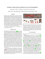
(a) Image+Scribbles (b) Node Uncertainty (c) Edge Uncertainty
(d) GC Uncertainty (e) Distance Transform (f) Intervening Contour
(g) Combining cues
Figure 3: Cues: (a) shows the image with provided scribbles; (b)-
(f) show various cues; and (g) shows how these cues are combined
to produce a final recommendation map.
and use the inverse of the entropy of this distribution as our
cue.
Codeword Distribution over Images (CD). This imagelevel
cue captures how diverse an image is, with the
motivation being that scribbling on images containing
more diversity among features would lead to better foreground/background
models. To compute this cue, we cluster
the features computed from all superpixels in the group
to form a codebook, and the confusion score for each image
is the entropy of the distribution over the codewords observed
in the image. The intuition is that the more uniform
the codeword distribution for an image the more diverse the
appearances of different regions in the image.
4.4. Combined Recommendation Map
We now describe how we combine these various cues
to produce a combined confusion map. Intuitively, the optimal
combination scheme would be one that generates a
recommendation map that assigns high values to regions
that a user would scribble on, if they were to exhaustively
examine all segmentations. Users typically scribble on regions
that are incorrectly segmented. We cast the problem
of learning the optimal set of weights for our cues, as that of
learning a linear classifier (logistic regression) that maps every
superpixel (represented by a 7-dimensional feature vector
corresponding to each of the 7 cues described above) to
the (binary) segmentation error-map. Our cue combination

scheme is illustrated in Figure 3.
5. The CMU-Cornell iCoseg Dataset
To evaluate our proposed approach and to establish a
benchmark for future work, we introduce the largest cosegmentation
dataset yet, the CMU-Cornell iCoseg Dataset.
While previous works have experimented with a few pairs
of images, our dataset contains 38 challenging groups with
643 total images (∼17 images per group), with associated
pixel-level ground truth. We built this dataset from the
Flickr® online photo collection, and hand-labelled pixellevel
segmentations in all images. We used the “Group”
feature in Flickr, where users form groups around popular
themes, to search for images from this theme. Our dataset
consists of animals in the wild (elephants, pandas, etc.),
popular landmarks (Taj Mahal, Stonehenge, etc.), sports
teams (Baseball, Football, etc.) and other groups that contain
a common theme or common foreground object. For
some (though not all) of the groups, we restricted the images
to come from the same photographer’s photo-stream,
making this a more realistic scenario. Examples of these
groups are shown in various figures in this paper and more
examples may be found online [3]. We note that this
dataset is significantly larger than those used in previous
works [13, 23]. We have made this dataset (and annotations)
publicly available [3] to facilitate further work, and
allow for easy comparisons.
6. Experiments
6.1. Machine Experiments
To conduct a thorough set of experiments and evaluate
various design choices, it is important to be able to perform
multiple iterations without explicitly polling a human
for scribbles. Thus, we develop a mechanism to generate
automatic scribbles, that mimic human scribbles (we also
present results of a user-study in Section 6.2). We model
these synthetic scribbles as (smooth) random walks that do
not cross foreground-background boundaries. Our scribble
generation technique consists of sampling a starting point
in the image uniformly at random. A direction angle is then
randomly sampled such that it is highly correlated with the
previous direction sample (for smoothness) for the scribble,
3 and a fixed-size (=30 pixels) step is taken along this
direction to extend the scribble (as long as it does not cross
object boundaries, as indicated by the groundtruth segmentation
of the image). To mimic user-scribbles given a recommendation
map, the initial as well as subsequent points
on the scribble are picked by considering the recommendation
map to be a distribution. Using synthetic scribbles
3 For the first two sampled points, there is no previous direction and this
direction is sampled uniformly at random.
(a) Image (b) Confusion Map
(c) Sampled Scribbles
Figure 4: Example simulated scribbles: Note that these scribbles
never cross foreground boundaries (red player).
Mean Rank
6
4
2
0
NU EU GC DT IC SS CD
Cue
Figure 5: Mean ranks achieved by individual cues (see Sec 6.1).
allows us to control the length of scribbles and observe the
behavior of the algorithm with increasing information. Example
synthetic scribbles are shown in Figure 4.
We first analyze the informativeness of each of our 7
cues. We start by generating a foreground and background
scribble on a random image in a group. We then compute
each of our cues, and treat each individual cue as a recommendation
map. We generate the next synthetic scribble as
guided by this recommendation map. We repeat this till we
have scribbled about 1000 pixels across the group, and compute
the average segmentation accuracy across the images
of a group. 4 We rank the 7 cues by this accuracy. Figure 5
shows the mean ranks (across groups, average of 10 random
runs) achieved by these cues. Out of our cues, the graph-cut
cue (GC) performs the best, while both distance transform
(DT) and intervening contour (IC) are the weakest.
We now evaluate iCoseg, our recommendation system,
as a whole. The experimental set up is the same as that
described above, except now we use the combined recommendation
map to guide subsequent scribbles (and not individual
cues). The cue combination weights are learnt from
all groups except one that we test on (leave-one-out cross
validation). We compare to two baselines. One is that of
using a uniform recommendation map on all images in the
4 In order to keep statistics comparable across groups, we select a random
subset of 5 images from all groups in our dataset. One of our groups
consisted of 4 images only, so all our results are reported on 37 groups.

Co−segmentation Acc. (%)
100
90
80
70
60
Upper Bound
iCoseg
Baseline (Uniform Rec. Map)
Baseline (single im.)
50
120 360 600 840 1080
Scribble Length (#pixels)
Figure 6: Machine Experiments: iCoseg significantly outperforms
baselines and is close to a natural upper-bound (Section 6.1).
group, which essentially means randomly scribbling on the
images (respecting object boundaries of course). And the
other (even weaker) baseline is that of selecting only one
image (randomly) in a group to scribble on (with a uniform
recommendation map on this image).
Figure 6 shows the performance of our combined recommendation
map (iCoseg) with increasing scribble length,
as compared to the baselines. We see that our proposed
recommendation scheme does in fact provide meaningful
guidance for regions to be scribbled on next (as compared
to the two baselines). A meaningful upper-bound would be
the segmentation accuracy that could be achieved if an oracle
told us where the segmentations were incorrect, and
subsequent scribbles were provided only in these erroneous
regions. As seen in Figure 6, iCoseg performs very close
to this upper bound, which means that users following our
recommendations can achieve cutout performances comparable
to those achieved by analyzing mistakes in all cutouts
with significantly less effort without ever having to examine
all cutouts explicitly.
6.2. User Study
In order to further test iCoseg, we developed a java-based
user-interface for interactive co-segmentation. 5 We conducted
a user study to verify our hypothesis that our proposed
approach can help real users produce good quality
cutouts from a group of images, without needing to exhaustively
examine mistakes in all images at each iteration. Our
study involved 15 participants performing 3 experiments
(each involving 5 groups of 5 related images). Figure 8
shows screen-shots from the three experiments. The sub-
5 We believe this interface may be useful to other researchers working
on interactive applications and we have made it publicly available [3].
Cosegmentation Acc. (%)
100
90
80
70
60
Exhaustive Examination (Exp 2)
iCoseg (Exp 3)
Random Scribbling (Exp 1)
50
120 360 600 840 1080
Scribble Length (#pixels)
Figure 7: User Study: Average performance of subjects in the
three conducted experiments (see Section 6.2). iCoseg (Exp. 3)
requires significantly less effort for users, e.g. allowing them to
reach 80% co-seg accuracy with three-fourth the effort of Exp. 1.
jects were informed that the first experiment was to acclimatize
them to the system. They could scribble anywhere
on any image, as long as they used blue scribbles on foreground
and red scribbles on background. The system computed
cutouts based on their scribbles, but the subjects were
never shown these cutouts. We consider this experiment to
be a replica of the random-scribble setup, thus forming a
lower bound for the active learning setup. In the second
experiment, the subjects were shown the cutouts produced
produced on all images in the group from their scribbles.
Their goal was to achieve 95% co-segmentation accuracy in
as few interactions as possible, and they could scribble on
any image. We observed that a typical strategy used by subjects
was to find the worst cutout at every iteration, and then
add scribbles to correct it. In the third experiment, they had
the same goal, but this time, while were shown all cutouts,
they were constrained to scribble within a window recommended
by our algorithm, iCoseg. This window position
was chosen by finding the location with the highest average
recommendation value (in the combined recommendation
map) in a neighbourhood of 201 × 201 pixels. The use of
a window was merely to make the user-interface intuitive,
and other choices could be explored.
Figure 7 shows the average segmentation accuracies
achieved by the subjects in the three experiments. We can
see that, as with the machine experiments, iCoseg helps
the users perform better than random scribbling, in that the
same segmentation accuracy (80%) can be achieved with
about three-fouth the effort (in terms of length of scribbles).
In addition, the average time taken by the users for one iteration
of scribbling reduced from 20.2 seconds (exhaustively
examining all cutouts) to 14.2 seconds (iCoseg), an aver-

(a) Experiment 1 (b) Experiment 2 (c) Experiment 3
Figure 8: User Study Screenshots: (a) Exp. 1: subjects were not shown cutouts and were free to scribble on any image/region while
respecting the foreground/background boundaries; (b) Exp. 2: subjects exhaustively examine all segmentations and scribble on mistakes
(cyan indicates foreground); (c) Exp. 3: users were instructed to scribble in the region recommended by iCoseg. Best viewed in colour.
age saving of 60 seconds per group. Thus, our approach
enables users to achieve cutout accuracies comparable to
those achieved by analyzing mistakes in all cutouts, in significantly
less time.
7. Conclusions
We present an algorithm for interactive co-segmentation
of a group of realistic related images. We propose iCoseg,
an approach that co-segments all images in the group using
an energy minimization framework, and an automatic
recommendation system that intelligently recommends a region
among all images in the group where the user should
scribble next. We introduce and make publicly available the
largest co-segmentation dataset, the CMU-Cornell iCoseg
dataset containing 38 groups (643 images), along with pixel
groundtruth hand annotations [3]. In addition to machine
experiments with synthetic scribbles, we perform a userstudy
on our developed interactive co-segmentation interface
(also available online), both of which demonstrate that
using iCoseg, users can achieve good quality segmentations
with significantly lower time and effort than exhaustively
examining all cutouts.
Acknowledgements: The authors would like to thank Yu-
Wei Chao for data collection and annotation, and Kevin
Tang for developing the java-based GUI (iScrrible) [3] used
in our user-studies.
References
[1] S. Bagon. Matlab wrapper for graph cut, December 2006.
[2] X. Bai and G. Sapiro. A geodesic framework for fast interactive
image and video segmentation and matting. In ICCV, 2007.
[3] D. Batra, A. Kowdle, D. Parikh, K. Tang, and T. Chen. http:
//amp.ece.cornell.edu/projects/touch-coseg/,
2009. Interactive Cosegmentation by Touch.
[4] D. Batra, R. Sukthankar, and T. Chen. Semi-supervised clustering
via learnt codeword distances. In BMVC, 2008.
[5] C. A. Bouman. Cluster: An unsupervised algorithm
for modeling Gaussian mixtures. Available from
http://www.ece.purdue.edu/˜bouman, April 1997.
[6] Y. Boykov and M.-P. Jolly. Interactive graph cuts for optimal boundary
and region segmentation of objects in n-d images. ICCV, 2001.
[7] Y. Boykov and V. Kolmogorov. An experimental comparison of mincut/max-flow
algorithms for energy minimization in vision. PAMI,
26(9):1124–1137, 2004.
[8] Y. Boykov, O. Veksler, and R. Zabih. Efficient approximate energy
minimization via graph cuts. PAMI, 20(12):1222–1239, 2001.
[9] B. Collins, J. Deng, K. Li, and L. Fei-Fei. Towards scalable dataset
construction: An active learning approach. In ECCV, 2008.
[10] D. Comaniciu and P. Meer. Mean shift: a robust approach toward
feature space analysis. PAMI, 24(5):603–619, 2002.
[11] A. Criminisi, T. Sharp, and A. Blake. Geos: Geodesic image segmentation.
In ECCV, 2008.
[12] J. Cui, Q. Yang, F. Wen, Q. Wu, C. Zhang, L. V. Gool, and X. Tang.
Transductive object cutout. In CVPR, 2008.
[13] D. S. Hochbaum and V. Singh. An efficient algorithm for cosegmentation.
In ICCV, 2009.
[14] D. Hoiem, A. A. Efros, and M. Hebert. Geometric context from a
single image. In ICCV, 2005.
[15] A. Kapoor, K. Grauman, R. Urtasun, and T. Darrell. Active learning
with gaussian processes for object categorization. In ICCV, 2007.
[16] P. Kohli and P. H. S. Torr. Measuring uncertainty in graph cut solutions.
CVIU, 112(1):30–38, 2008.
[17] V. Kolmogorov and R. Zabih. What energy functions can be minimized
via graph cuts? PAMI, 26(2):147–159, 2004.
[18] T. Leung and J. Malik. Contour continuity in region based image
segmentation. In ECCV, 1998.
[19] Y. Li, J. Sun, C.-K. Tang, and H.-Y. Shum. Lazy snapping. SIG-
GRAPH, 2004.
[20] Y. Mu and B. Zhou. Co-segmentation of image pairs with quadratic
global constraint in mrfs. In ACCV, 2007.
[21] L. Mukherjee, V. Singh, and C. R. Dyer. Half-integrality based algorithms
for cosegmentation of images. In CVPR, 2009.
[22] C. Rother, V. Kolmogorov, and A. Blake. “Grabcut”: interactive
foreground extraction using iterated graph cuts. SIGGRAPH, 2004.
[23] C. Rother, T. Minka, A. Blake, and V. Kolmogorov. Cosegmentation
of image pairs by histogram matching - incorporating a global
constraint into mrfs. In CVPR, 2006.
[24] Y. Schnitman, Y. Caspi, D. Cohen Or, and D. Lischinski. Inducing
semantic segmentation from an example. In ACCV, 2006.
[25] B. Settles. Active learning literature survey. Computer Sciences
Technical Report 1648, University of Wisconsin–Madison, 2009.
[26] H. S. Seung, M. Opper, and H. Sompolinsky. Query by committee.
In COLT, 1992.
[27] S. Vijayanarasimhan and K. Grauman. What’s it going to cost you?:
Predicting effort vs. informativeness for multi-label image annotations.
In CVPR, 2009.
[28] R. Yan, J. Yang, and A. Hauptmann. Automatically labeling video
data using multi-class active learning. In ICCV, 2003.