Conditioning reduces entropy Prediction by partial matching ... - CIM

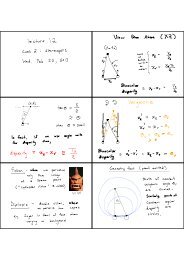
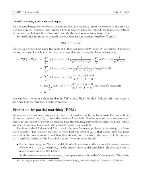
COMP 423 lecture 16 Feb. 11, 2008 

Conditioning reduces entropy 

We are considering how to encode the next symbol in a sequence, given the context of the previous 

k symbols in the sequence. Our intution here is that by using the context, we reduce the entropy 

of the next symbol and this allows us to encode the next symbol using fewer bits. 

To justify this intuition to yourself, observe that for any random variables X and Y , 

H(X|Y ) ≤ H(X) 

that is, on average if we know the value of Y then our uncertainty about X is reduced. The proof 

is easy, once you know how to set it up in a way that you can apply Jensen’s inequality: 

H(X|Y ) − H(X) = 

1 

1 

p(X = i, Y = j) log 

− p(X = i) log 

p(X = i|Y = j) p(X = i) 

X,Y 

= 

p(Y = j) 

p(X = i, Y = j)(log 

+ log p(X = i)) 

p(X = i, Y = j) 

X,Y 

= 

p(X = i, Y = j)(log 

X,Y 

≤ log 

= 0. 

X,Y 

p(Y = j)p(X = i) 

p(X = i, Y = j) ) 

p(Y = j)p(X = i) 

p(X = i, Y = j) 

p(X = i, Y = j) , by Jensen′ s inequality 

One subtlety: we are not claiming that H(X|Y = j) ≤ H(X) for all j. Indeed such a statement is 

not true. (Try to construct a counterexample.) 

Prediction by partial matching (PPM) 

Suppose we are encoding a sequence X1, X2, . . .,Xn and we are trying to estimate the probabilities 

of the next symbol, say Xj+k given the previous k symbols. If some symbols have never occured 

before in this context of k symbols, then we have the zero frequency problem mentioned last lecture. 

We don’t know how to estimate the probabilities of these symbols. 

The idea of the PPM method 1 is to avoid the zero frequency problem by switching to a lower 

order context. The encoder tells the decoder that the symbol Xj+k that comes next has never 

occured in the present context, and that they should (both) switch to the context of the previous 

k − 1 symbols, instead of the k symbol context. Here are some details: 

• Rather than using one Markov model of order k, use several Markov models, namely, models 

of order 0, 1, . . ., kmax, where kmax is the largest order model considered. (In fact, an order -1 

model is used as well. See below.) 

As the encoder encodes the sequence, it computes counts for each of these models. This allows 

1 See the original paper, which is relatively easy to read: http://www.cim.mcgill.ca/˜langer/423/PPM.pdf 

1 

X


it to compute conditional probability functions: 

p(next symbol | previous kmax symbols ) 

p(next symbol | previous kmax − 1 symbols ) 

. 

p(next symbol | previous symbol ) 

p(next symbol ) 

• Add one more symbol, AN+1 = ǫ (for “escape”) to the alphabet. This escape symbol indicates 

that the encoder is switching from the k th order model to the k − 1 th order model. 

• To choose the probabilities of the next symbol, use the highest order model k such that the 

previous k symbols followed by the next symbol has occured at least once in the past. That 

is, the encoder keeps escaping until it finds such an order. 

• What if a symbol has never occured before in any context? That is, what if it is the first 

time that a symbol occurs? In this case, the encoder uses a “k = −1” order model to encode 

the symbol. (Call the order “-1” is meaningless, of course. All this means is that we are 

decrementing the order from k = 0, i.e. we escaped from k = 0.) 

Example 1: “abracadabra” with kmax = 2 

The symbols that are encoded are: 

and corresponding orders are 

ǫ, ǫ, ǫ, a, ǫ, ǫ, ǫ, b, ǫ, ǫ, ǫ, r, ǫ, ǫ, a, ǫ, ǫ, ǫ, c, ǫ, ǫ, a, ǫ, ǫ, ǫ, d, ǫ, ǫ, a, ǫ, b, r, a 

2, 1, 0, −1, 2, 1, 0, −1, 2, 1, 0, −1, 2, 1, 0, 2,1, 0, −1, 2, 1,0, 2, 1, 0, −1, 2, 1, 0, 2, 1,2, 2 

You may wonder how this could achieve compression. The number of symbols (including the ǫ) 

is far more than the original number of symbols. On the one hand, one would think that this would 

require more bits! On the other hand, notice that many of these “escapes” occur with probability 

1 and so no bits need to be sent. 

Example 2 

Let {a,b} be the alphabet and kmax = 1. Suppose the string we wish to encode begins aabb... 

We send the following symbols: 

ǫ, ǫ, a, ǫ, a, ǫ, ǫ, b, ǫ, b, .. 

Let’s consider, for each of these symbols, the probabilities for a, b, ǫ. In the table below, we 

consider only those cases where the probability is 0 or 1. 

2


order of model 1 0 -1 1 0 1 0 -1 1 0 

p(a) 0 0 0 0 ∗ 0 ∗ 0 

p(b) 0 0 0 0 0 0 0 

p(ǫ) 1 1 1 1 1 

encode symbol ǫ ǫ a ǫ a ǫ ǫ b ǫ b ... 

Only symbols that have been seen before in the current context (previous k symbols) can be 

encoded in this context. If Ai hasn’t been seen in the current context we assign its probability to 

0 and we encode ǫ instead. The ǫ tells the decoder that the symbol that comes next is one of the 

symbols that has not been seen before in the current context. 

What does it mean to send ǫ at k = −1 ? This could be used to indicate the end of the sequence 

(EOF). It is not obvious now why we need to explicitly encode EOF. Indeed if we were to Huffman 

code the next symbol, then we would not need an EOF. Next week we will see a method, called 

arithmetic coding, where we do need to explicitly code EOF. We do so by escaping from the order 

k = −1 model. 

Exclusion Principle 

The entries with an asterisk ( ∗ ) in the above table are rather subtle. For these entries, we are 

claiming that the probability of encoding that symbol is 0. (The symbol is an a in these cases.) 

Why? The reason is that, if the next symbol were an a then it would never have reached the current 

order model because it would have been encoded using a higher order model. For example, take the 

case of the third symbol in the sequence (which happens to be b). If the third symbol had instead 

been ”a”, then at the k = kmax = 1 step, the symbol ”a” would have been encoded (rather than 

ǫ) because an ”a” in the context of an ”a” had occured previously (namely, the first and second 

symbols of the sequence). Because ǫ was encoded at that step, the decoder can infer that the third 

symbol is not ”a” and so ”a” is given zero probability. The same argument applies at the k = −1 

model. Because ”a” had occurred previously (order k = 0), if the next symbol were ”a” then we 

would not have escaped from k = 0 to k = −1. 

This interesting idea is called the Exclusion Principle. Formally, this Exclusion Principle is as 

follows. Suppose the encoder/decoder are trying to estimate 

where 

If 

p( encode Ai | previous k symbols) 

k < kmax . 

ct[ Ai | previous k + 1 symbols ] > 0 

then the encoder/decoder should assign p(encodeAi) := 0. 

There are two important points to note: 

• the Exclusion Principle does not apply at k = kmax. Rather, it applies only when the encoder 

has already escaped from a higher order model to a lower one. 

3


• The encoder/decoder are determining p( encode Ai) at within the k th order model. They 

are not determining p(Ai is the next symbol in the sequence). In particular, we could have 

p(encode Ai) = 0, but p(Ai is the next symbol in the sequence ) > 0. This would happen, 

for example, if symbol Ai had not occured before in this k th order context, but the next symbol 

in the sequence is indeed Ai (in which case, an ǫ would be encoded). 

Estimating probabilities from count frequencies 

Suppose we are in a context of an order k model and we wish to compute probabilities that each of 

the Ai’s and ǫ is encoded in this context. The way that we do it depends on k: 

estimate probability of encoding next symbol in context k(){ 

sum := weightescape; // fixed constant > 0 

for i = 1 to N { 

if (k == kmax) 

ct(i) := ct( Ai | previous k) 

else if (k ≥ 0) 

ct(i) := (ct( Ai | previous k + 1) == 0) * ct( Ai | previous k symbols); 

else 

ct(i) := (ct( Ai) == 0); 

sum += ct(i); 

} 

for i = 1 to N 

p(encode Ai) := ct(i) / sum; 

p(encode ǫ) := weightescape / sum; 

} 

Example 2 

We continue on with the example from earlier. We were considering the PPM method applied to a 

string that begins aabb.. with kmax = 1. The table that we saw last lecture was incomplete. We 

only marked off those entries that occur with probability 0 or 1. Let us now complete the table 

using the method just described. (The asterisk ∗ indicates that the Exclusion Principle was applied.) 

order of model 1 0 -1 1 0 1 0 -1 1 0 

1 1 

p( encode a) 0 0 0 3 2 

1 0 2 ∗ 0∗ 1 0 2 

1 

1 1 

p( encode b) 0 0 0 0 0 0 0 3 2 4 

p( encode ǫ) 1 1 

1 

3 1 

1 

2 

1 

2 1 

1 

2 1 

encode ǫ ǫ a ǫ a ǫ ǫ b ǫ b ... 

4 

1 

4

Conditioning reduces entropy Prediction by partial matching ... - CIM

You also want an ePaper? Increase the reach of your titles

Delete template?

Save as template?