MECH 314 Rolling without Slipping 7-Bar Mechanism Velocity ... - CIM

1 Position Analysis
MECH 314
Dynamics of Mechanisms
September 27, 2010
Rolling without Slipping 7-Bar Mechanism Velocity Analysis
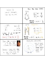
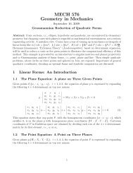
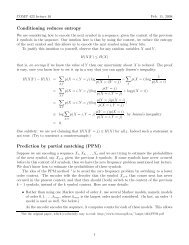
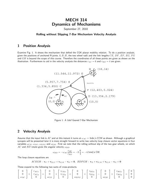
Examine Fig. 1. It shows the mechanism that defied the CGK planar mobility relation. To do a position analysis,
given the positions of anchored R-joints A, B, H, the two wheel radii and the link lengths CE, DF , EF , EG, F G
and GH is beyond the scope of this course. Therefore the coordinates of all these points are given as shown on the
illustration. Furthermore to aid in the velocity analysis the distances rAC = 6 and rBD = 4 are given.
(1.334,5.850) C
2 Velocity Analysis
(0,0)
(11.544,11.972) G
(5.957,7.754)
3s -1
A
AC
E
B
H
RwoS09z
F (12,403,5.024)
D
(10,0)
Figure 1: A 1dof Geared 7-Bar Mechanism
(16,14)
(13,354,2.179)
Assume that the input link is AC and at this instant it turns at ωAC = 3rdn/s CCW as shown. Although a graphical
synopsis will be presented later it is more straight forward to write two velocity loop closure vector equations in four
variables ωCE, ωDF , ωEF G and ωGH. First we note that the rolling without slip of the two gear wheels, on which
AC and BD rotate gives the angular velocity ωBD.
The loop closure equations are
ωAC
rAC
ωBD = −ωAC
rBD
= −3 6
= −4.5rnd/s CW
4
ACEGH : vC + v E/C + v G/E − vG = 0, BDF GH : vD + v F/D + v G/F − vG = 0
These expand to the following two sums of cross-products.
⎡ ⎤ ⎡ ⎤ ⎡ ⎤ ⎡ ⎤ ⎡
0 rACx 0 rCEx 0
⎣ 0 ⎦ × ⎣ ⎦ + ⎣ 0 ⎦ × ⎣ ⎦ + ⎣ 0
rACy
0
ωCE
rCEy
0
ωEF G
⎤
⎡
⎦ × ⎣
rEGx
rEGy
0
⎤
⎡
⎦ − ⎣
0
0
ωGH
⎤
⎡
⎦ × ⎣
rHGx
rHGy
0
⎤
⎡
⎦ = ⎣
0
0
0
⎤
⎦

2
⎡
⎣
0
0
ωBD
⎤
⎡
⎦ × ⎣
rBDx
rBDy
0
⎤
⎡
⎦ + ⎣
0
0
ωDF
⎤
⎡
⎦ × ⎣
rDF x
rDF y
0
⎤
⎡
⎦ + ⎣
0
0
ωEF G
⎤
⎡
⎦ × ⎣
rF Gx
rF Gy
0
⎤
⎡
⎦ − ⎣
0
0
ωGH
⎤
⎡
⎦ × ⎣
rHGx
rHGy
0
⎤
⎡
⎦ = ⎣
These lead to a detached coefficient form of four simultaneous linear equations in five homogeneous variables
⎡
−ωACrACy
⎢ ωACrACx ⎢
⎣ −ωBDrBDy
ωBDrBDx
−rCEy
rCEx
0
0
0
0
−rDF y
rDF x
−rEGy
rEGx
−rF Gy
rF Gx
rHGy
−rHGx
rHGy
−rHGx
⎡
⎤ ∆
⎢ ΩCE ⎥ ⎢
⎥ ⎢ ΩDF ⎦ ⎢
⎣ ΩEF G
⎤
⎥
⎦ =
⎡ ⎤
0
⎢ 0 ⎥
⎢ 0 ⎥
⎣ 0 ⎦
0
such that
where
ΩGH
ωCE = ΩCE
∆ , ωDF = ΩDF
∆ , ωEF G = ΩEF G
∆ , ωGH = ΩGH
∆
∆ =
ΩCE = −
ΩDF =
ΩEF G = −
ΩGH =
−rCEy 0 −rEGy rHGy
rCEx 0 rEGx −rHGx
0 −rDF y −rF Gy rHGy
0 rDF x rF Gx −rHGx
−ωACrACy 0 −rEGy rHGy
ωACrACx 0 rEGx −rHGx
−ωBDrBDy −rDF y −rF Gy rHGy
ωBDrBDx rDF x rF Gx −rHGx
−ωACrACy −rCEy −rEGy rHGy
ωACrACx rCEx rEGx −rHGx
−ωBDrBDy 0 −rF Gy rHGy
ωBDrBDx 0 rF Gx −rHGx
−ωACrACy −rCEy 0 rHGy
ωACrACx rCEx 0 −rHGx
−ωBDrBDy 0 −rDF y rHGy
ωBDrBDx 0 rDF x −rHGx
−ωACrACy −rCEy 0 −rEGy
ωACrACx rCEx 0 rEGx
−ωBDrBDy 0 −rDF y −rF Gy
ωBDrBDx 0 rDF x rF Gx
The link vectors are obtained by subtracting the coordinates of the first point subscript from the second, e.g.,
differences of point position vectors such as rAC = c − a.
⎡ ⎤
1.334
⎡
4.623
⎤ ⎡ ⎤
5.587
rAC = ⎣ 5.850 ⎦ , rCE = ⎣ 1.904 ⎦ , rEG = ⎣ 4.218 ⎦
⎡ ⎤
3.354
0
⎡ ⎤
−0.951
0
⎡ ⎤
−0.859
0
⎡
−4.456
⎤
rBD = ⎣ 2.179 ⎦ , rDF = ⎣ 2.845 ⎦ , rF G = ⎣ 6.948 ⎦ , rHG = ⎣ −2.028 ⎦
0
0
0
0
3 Results and a Graphical Check
Substituting the numerical values for the parameters in the detached coefficient matrix yields
⎡
⎢
⎣
−17.55
4.002
9.8055
−1.904
4.623
0
0
0
−2.845
−4.218
5.587
−6.948
⎤
−2.028
4.456 ⎥
−2.028 ⎦
−15.093 0 −0.951 −0.859 4.456
0
0
0
⎤
⎦

Taking all 4 × 4 sub-matrix determinants with alternating sign and dividing the last four by the first produces the
unknown angular velocities.
vCy
ωCE = 4.0055, ωDF = 20.846, ωEF G = −8.9105, ωGH = 6.1184
The five point velocity vectors are calculated as follows.
vCx
−ωACrACy
=
−17.55
=
4.002
,
vEx
vEy
ωACrACx
vDx
vDy
=
−ωBDrBDy
ωBDrBDx
vCx − ωCErCEy −25.1765 vGx
=
=
, =
vCy + ωCErCEx 22.5195 vGy
vF x vDx − ωDF rDF y −49.5023
=
=
−34.9179
vF y
vDy + ωDF rDF x
−ωGHrHGy
ωGHrHGx
=
9.8095
−15.093
=
12.4082
−27.26373
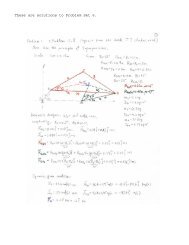
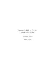
These results are checked by plotting the triangle EF G and projecting the velocity vectors vE, vF and vG onto the
respective triangle sides. Analytically these projections vE=, vF = and vG= would be dot-product operations. All
this has been done in Fig. 2 and the magnitudes of the projected vector pairs at either end of a side are compared.
Notice the good agreement. Discrepancy is largely due to three-place precision of the coordinates of the three points
that were given a-priori.
v EF= @E=31.966
v EF= @F=31.964
v EG= @E=6.528
v EG= @G=6.521
v FG= @F=28.582
v FG= @G=28.580
v F
v EF=
v E
v EG=
E
7BrRB091
Figure 2: Checking the Results of the Velocity Analysis
F
G
v FG=
v G
3