

The Picard-Lefschetz theory of complexified Morse functions 1 ...
The Picard-Lefschetz theory of complexified Morse functions 1 ...
The Picard-Lefschetz theory of complexified Morse functions 1 ...

You also want an ePaper? Increase the reach of your titles
YUMPU automatically turns print PDFs into web optimized ePapers that Google loves.
<strong>The</strong> <strong>Picard</strong>-<strong>Lefschetz</strong> <strong>theory</strong> <strong>of</strong> <strong>complexified</strong> <strong>Morse</strong> <strong>functions</strong><br />
JOE JOHNS<br />
Given a closed manifold N and a self-indexing <strong>Morse</strong> function f : N −→ R with<br />
up to four distinct <strong>Morse</strong> indices, we construct a symplectic <strong>Lefschetz</strong> fibration<br />
π : E −→ C which models the complexification <strong>of</strong> f on the disk cotangent bundle,<br />
fC : D(T ∗ N) −→ C, when f is real analytic. By construction, π : E −→ C comes<br />
with an explicit regular fiber M and vanishing spheres V1, . . . , Vm ⊂ M, one for<br />
each critical point <strong>of</strong> f . Our main result is that π : E −→ D 2 is a good model<br />
for fC : D(T ∗ N) −→ C in the sense that N embeds in E as an exact Lagrangian<br />
submanifold, and in addition, π|N = f and E is homotopy equivalent to N . <strong>The</strong>re<br />
are several potential applications in symplectic topology, which we discuss in the<br />
introduction.<br />
1 Introduction<br />
Complexifications in various forms have been considered for some time in many different<br />
fields, as in for example [B], [G68], [K78], [LS91], [AC99], [AMP05]. <strong>The</strong><br />
central problem is usually to understand the relation between the <strong>complexified</strong> object<br />
and its real counter part. In this paper we are concerned with the relation between<br />
<strong>Morse</strong> <strong>functions</strong> and their complex versions, <strong>Lefschetz</strong> fibrations. Historically, <strong>Morse</strong><br />
<strong>functions</strong> have <strong>of</strong> course played a central role in elucidating the differential topology<br />
<strong>of</strong> manifolds. On the other hand, <strong>Lefschetz</strong> fibrations played a large role in the<br />
study <strong>of</strong> the topology <strong>of</strong> algebraic varieties. <strong>The</strong>y have a formally similar definition<br />
to <strong>Morse</strong> <strong>functions</strong> (they are proper holomorphic maps on complex analytic varieties<br />
with generic singularities modeled on z2 1 + ... + z2n ), but they are in fact quite different<br />
in flavour. <strong>The</strong> most obvious difference one can point to is that <strong>Morse</strong> <strong>functions</strong> have<br />
regular level sets which differ in topological type, whereas all the regular fibers <strong>of</strong> a<br />
<strong>Lefschetz</strong> fibrations are diffeomorphic. (See, for example, [B89], [L81] for surveys <strong>of</strong><br />
<strong>Morse</strong> <strong>theory</strong> and the <strong>theory</strong> <strong>of</strong> <strong>Lefschetz</strong> fibrations.)<br />
Here is one way to complexify a <strong>Morse</strong> function to get a <strong>Lefschetz</strong> fibration. (Actually,<br />
the method we now present is somewhat naive, see remark 1.3, but it serves as a useful
2 Joe Johns<br />
starting point.) Suppose that N is a real analytic manifold and f : N −→ R is a real<br />
analytic <strong>Morse</strong> function. <strong>The</strong>n, in local charts on N , f is represented by some convergent<br />
power series with real coefficients; if we complexify these local power series<br />
to get complex analytic power series (with the same coefficients) we obtain a complex<br />
analytic map on the disk bundle <strong>of</strong> T ∗ N <strong>of</strong> some small radius ǫ > 0,<br />
fC : Dǫ(T ∗ N) −→ C,<br />
called the complexification <strong>of</strong> f . In favorable circumstances, fC can be regarded as a<br />
<strong>Lefschetz</strong> fibration. (<strong>The</strong> main issue which may prevent fC from being a <strong>Lefschetz</strong><br />
fibration is that parts <strong>of</strong> some fibers may be “missing”; this will happen if the parallel<br />
transport vector-field between regular fibers is incomplete. See remark 1.3 for more on<br />
this.) Actually, we want to think <strong>of</strong> fC as a symplectic <strong>Lefschetz</strong> fibration, which is an<br />
extension <strong>of</strong> the notion to the symplectic category due to Donaldson (see [D96, D99]).<br />
<strong>The</strong>re are some slightly different possible definitions and we follow the one in [S03A]<br />
(which also satisfies the definition in [S08A]); this is designed for work in the category<br />
<strong>of</strong> exact symplectic manifolds (with nonempty boundary). Roughly, a symplectic <strong>Lefschetz</strong><br />
fibration π : E −→ C is a fiber bundle with symplectic fibers, but with some<br />
isolated singular points modeled on z 2 1 + ... + z2 n.<br />
It is natural to ask: To what extent can the complex topology <strong>of</strong> fC be described<br />
in terms <strong>of</strong> the <strong>Morse</strong> <strong>theory</strong> <strong>of</strong> f ? <strong>The</strong> central problem here is to analyze the <strong>Picard</strong>-<br />
<strong>Lefschetz</strong> <strong>theory</strong> <strong>of</strong> fC, and we are particularly interested the symplectic view point (as<br />
opposed to classical topology, which deals with cycles):<br />
Problem 1.1 Describe the generic fiber <strong>of</strong> fC as a symplectic manifold M, and describe<br />
its vanishing cycles as Lagrangian spheres in M.<br />
Basically this entails reconstructing the picture <strong>of</strong> the regular complex fiber M starting<br />
only with knowledge <strong>of</strong> the <strong>Morse</strong> <strong>theory</strong> on the real part N ⊂ T ∗ N . This problem is<br />
very natural from the point <strong>of</strong> view <strong>of</strong> singularity <strong>theory</strong>, and indeed our approach is<br />
greatly influenced by work <strong>of</strong> A’Campo [AC99] which treats the case where f is a real<br />
polynomial on N = R 2 , and fC : C 2 −→ C is the same polynomial on C 2 .<br />
In our approach we first take a Riemannian metric g such that (f, g) is <strong>Morse</strong>-Smale<br />
and we only assume (N, f, g) is smooth, not necessarily real analytic. Given the corresponding<br />
handle decomposition <strong>of</strong> N , we construct an exact symplectic manifold M <strong>of</strong><br />
dimension 2dim N −2 together with some exact Lagrangian spheres L1,... , Lm ⊂ M,<br />
one for each critical point <strong>of</strong> f . <strong>The</strong>n, given (M, L1,...,Lm), there is a unique (up to deformation)<br />
symplectic <strong>Lefschetz</strong> fibration π : E −→ C, with generic fiber M = π −1 (b)
Complexified <strong>Morse</strong> <strong>functions</strong> 3<br />
and vanishing spheres L1,... , Lm (see [S08A, §16e]). <strong>The</strong>orem A below shows that<br />
(E,π) and (D(T ∗ N), fC) have the same key features. In this sense (E,π) is a good<br />
model for (D(T ∗ N), fC) and (M, L1,... , Lm) is very likely a correct answer to problem<br />
1.1. In any case, for applications (see section §1.3) we need not use fC; instead we<br />
will always use (E,π). Thus the question <strong>of</strong> whether E ∼ = D(T ∗ N) and π ∼ = fC is not<br />
pressing for the moment; still this question remains an interesting one and we intend<br />
to pursue it in future work, see remark 1.3 below for more on that.<br />
<strong>The</strong>orem A Assume N is a smooth closed manifold and f : N −→ R is self-indexing<br />
<strong>Morse</strong> function with either two, three, or four critical values: {0, n}, {0, n, 2n}, or<br />
{0, n, n+1, 2n+1}. Let (M, L1 ...,Lm) be the data from the construction we discussed<br />
above (which depends in addition on a Riemannian metric g on N such that (f, g) is<br />
<strong>Morse</strong>-Smale). Let π : E −→ C be the corresponding symplectic <strong>Lefschetz</strong> fibration<br />
with fiber M and vanishing spheres (L1,...,Lm). <strong>The</strong>n, N embeds in E as an exact<br />
Lagrangian submanifold so that:<br />
• all the critical points <strong>of</strong> π lie on N , and in fact Crit(π) = Crit(f );<br />
• π(N) is a closed subinterval <strong>of</strong> R; and,<br />
• π|N = f : N −→ R (up to reparameterizing N and R by diffeomorphisms).<br />
<strong>The</strong>orem A appears below as <strong>The</strong>orem 8.1. As a step towards proving E ∼ = D(T ∗ N),<br />
we also give a fairly detailed sketch that E is homotopy equivalent to N in Proposition<br />
8.4. (See also remark 1.3 for a different sketch <strong>of</strong> the stronger statement, E ∼ = D(T ∗ N),<br />
which is less detailed.)<br />
Remark 1.2 <strong>The</strong> contruction <strong>of</strong> (M, L1,... , Lm) and (E,π), and the pro<strong>of</strong> <strong>of</strong> <strong>The</strong>orem<br />
A, all work equally well for non-closed manifolds N .<br />
<strong>The</strong> main point <strong>of</strong> <strong>The</strong>orem A is the construction <strong>of</strong> the exact Lagrangian embedding<br />
N ⊂ E. <strong>The</strong> other conditions on N are rather natural, and in fact their main use here is<br />
to guide the construction <strong>of</strong> N ⊂ E. <strong>The</strong> hypotheses on f ensure that the contruction <strong>of</strong><br />
M is relatively easy. In a sequel paper, to appear later, we will give a detailed treatment<br />
<strong>of</strong> the construction <strong>of</strong> M in general, which is more complicated. (See §3.4 <strong>of</strong> this<br />
paper for a partial sketch <strong>of</strong> that.) <strong>The</strong> pro<strong>of</strong> <strong>of</strong> <strong>The</strong>orem A will then carry over easily<br />
to the general case. (Indeed, even in this paper our pro<strong>of</strong> <strong>of</strong> <strong>The</strong>orem A focuses first<br />
on the case where f has just three <strong>Morse</strong> indices (see §4-8). <strong>The</strong>n we explain how the<br />
pro<strong>of</strong> carries over easily to the case where f has four <strong>Morse</strong> indices in §9.) Later, we<br />
will also flesh out the ideas relating (D(T ∗ N), fC) and (E,π) sketched in remark 1.3<br />
below. For more about the contents and organization <strong>of</strong> this paper, see §1.1 below.
4 Joe Johns<br />
Remark 1.3 <strong>The</strong> precise relationship <strong>of</strong> π to fC is not so obvious, first, because π<br />
apparently depends on the metric g whereas fC does not, and second, because π can<br />
arise from non-analytic data (f, g), whereas fC must have an analytic datum f . Finally,<br />
and most importantly, fC is not really a <strong>Lefschetz</strong> fibration in the strict sense if one<br />
constructs it in the naive way we described. <strong>The</strong> reason is the regular fibers <strong>of</strong> fC<br />
are not going to be diffeomorphic. Indeed, for a given real regular value x ∈ R, the<br />
complex level set f −1<br />
C (x) will be symplectomorphic to D(T∗ (f −1 (x))), which is the disk<br />
cotangent bundle <strong>of</strong> the corresponding real level set f −1 (x). But this fiber is much too<br />
small: If fC was a <strong>Lefschetz</strong> fibration with complete parallel transport vector fields<br />
(where the connection is given by the symplectic orthogonal to the fibers), then all the<br />
regular fibers would be symplectomorphic, hence each regular fiber should contain all<br />
the real regular level sets <strong>of</strong> f as Lagrangian submanifolds (because we could parallel<br />
transport all these Lagrangian submanifolds into any fixed regular fiber). One can<br />
think <strong>of</strong> π : E −→ C as a larger (genuine) <strong>Lefschetz</strong> fibration which does have this<br />
property. We conjecture that the correct picture relating (E,π) and (D(T ∗ N), fC) is<br />
that D(T ∗ N) embeds into E as a kind <strong>of</strong> diagonal subset intersecting each regular<br />
fiber π −1 (x), x ∈ R, in a Weinstein neighborhood <strong>of</strong> the real level set f −1 (x), as we<br />
said before. <strong>The</strong>n E should be conformally exact symplectomorphic to D(T ∗ N) by<br />
a retraction along a Liouville type vector field (namely, a variably re-scaled version<br />
<strong>of</strong> the symplectic lift <strong>of</strong> ∂<br />
∂x from the real line), and π|D(T ∗ N) should be deformation<br />
equivalent to fC.<br />
1.1 Overview<br />
<strong>The</strong> main purpose <strong>of</strong> this paper is to prove <strong>The</strong>orem A, see <strong>The</strong>orem 8.1 below. <strong>The</strong>re<br />
are three steps in the pro<strong>of</strong>. First, in § 3, we construct the regular fiber M and vanishing<br />
spheres L1,... , Lm. (<strong>The</strong> construction is based on some techniques explained in §2.)<br />
Second, in §4-7, we construct a symplectic <strong>Lefschetz</strong> fibration π : E −→ D 2 with this<br />
regular fiber and these vanishing spheres. (See § 1.1.1 to see why this construction is<br />
not immediate.) Third, in §8, we construct an exact Lagrangian embedding N ⊂ E<br />
satisfying the conditions in <strong>The</strong>orem A. (See §1.1.2 for a sketch.)<br />
Once the construction <strong>of</strong> N ⊂ E is carried out in detail in one particular case, it<br />
is straight-forward to see how it works in any other case. For this reason we first<br />
concentrate on the case where f has three distinct <strong>Morse</strong> indices 0, n, 2n, focusing<br />
on the case where dim N = 4; this takes up the bulk <strong>of</strong> the paper, §4-8. In §9 we<br />
explain how the pro<strong>of</strong> carries over easily to the case when f has four distinct <strong>Morse</strong>
Complexified <strong>Morse</strong> <strong>functions</strong> 5<br />
indices 0, n, n + 1, 2n + 1, focusing on the case dim N = 3. In general, for any fixed<br />
number <strong>of</strong> <strong>Morse</strong> indices for f , all three steps in the pro<strong>of</strong> are essentially the same as<br />
the dimension <strong>of</strong> N varies. (See §3.2, for example, to see why this is so.) That is why<br />
we look at the slightly more concrete cases where dim N = 4 and dim N = 3. (We<br />
focus on the case dim N = 4 rather than dim N = 2 because the latter case is actually<br />
a little confusing from the general point <strong>of</strong> view, because <strong>of</strong> its very low dimension.)<br />
Remark 1.4 As it happens, closed 4-manifolds admitting handle decompositions<br />
without 1- and 3-handles form a fairly rich class <strong>of</strong> examples. This class includes CP 2 ,<br />
CP 2 , and elliptic surfaces (assuming simply-connected with sections, see [GS99]), and<br />
it is closed under connected sum (so blow up in particular). It is not known if it includes<br />
all simply-connected closed 4-manifolds, or even all hypersurfaces in CP 3 ; this has<br />
been a long standing question. (Recently, however, a famously conjectured counterexample,<br />
the Dolgachef surface [HKK89], has been proved by Akbulut [A08] to be in<br />
this class as well.) See [HKK89], [K89], [GS99] for more extensive discussions.<br />
1.1.1 Sketch <strong>of</strong> the construction <strong>of</strong> (E,π)<br />
Given (M, L1,...,Lm) there is a standard (and fairly easy) construction for producing<br />
a <strong>Lefschetz</strong> fibration with fiber M and vanishing spheres L1,... , Lm. (See [S08A,<br />
§16e].) We, however, construct (E,π) in a different, more explicit, way in order to<br />
facilitate the construction <strong>of</strong> N ⊂ E. Actually, most <strong>of</strong> the difficulty for us is concentrated<br />
in this non-standard construction <strong>of</strong> (E,π) (see §4-7) after which the contruction<br />
<strong>of</strong> N ⊂ E is relatively easy (see §8).<br />
Our strategy for constructing (E,π) is as follows. For simplicity <strong>of</strong> notation assume<br />
that f has just one critical point <strong>of</strong> each index, say x0, x2, x4 . Our aim is for<br />
π : E −→ D 2 to have exactly three critical values c0 < c2 < c4; these will lie on the<br />
real line and correspond to the critical values <strong>of</strong> f . We first construct three <strong>Lefschetz</strong><br />
fibrations, one for each critical value ci :<br />
πi : Ei −→ Ds(ci), i = 0, 2, 4,<br />
where Ds(ci) is a small disk around ci <strong>of</strong> radius s > 0. <strong>The</strong> aim is to construct<br />
(E,π) so that (Ei,πi) is equal to the restriction <strong>of</strong> π to a small disk around ci , namely<br />
(E|Ds(ci),π|Ds(ci)) = (Ei,πi). Each πi will have a unique critical point, say xi , with just<br />
one vanishing sphere corresponding to xi . In this case there is a standard construction<br />
(namely [S03A, lemma 1.10]) which we use to produce each πi (see §5). <strong>The</strong> regular
6 Joe Johns<br />
fiber <strong>of</strong> each πi , say Mi, will be exact symplectomorphic to M. <strong>The</strong> key new ingredient<br />
in our construction <strong>of</strong> (E,π) is a twisting operation<br />
M T ±π/2(M)<br />
that we use to define M2 = T π/2(M). (See §5.3 for the definition <strong>of</strong> this twisting<br />
operation; we will explain its main properties in a moment.) By construction, π0,π2,π4<br />
have regular fibers given by canonical isomorphisms as follows:<br />
π −1<br />
0 (c0 + s) ∼ = M,<br />
π −1<br />
2 (c2 + s) ∼ = M2,<br />
π −1<br />
4 (c4 − s) ∼ = M2.<br />
<strong>The</strong> main point <strong>of</strong> the twisting operation M T π/2(M) is that there is a canonical<br />
isomorphism π −1<br />
2 (c2−s) ∼ = M (see lemma 6.1) and a natural exact symplectomorphism<br />
τ : M −→ M2 = T π/2(M)<br />
such that, under the canonical isomorphisms π −1<br />
2 (c2 − s) ∼ = M and π −1<br />
2 (c2 + s) ∼ = M2,<br />
τ coresponds precisely to the symplectic transport map<br />
π −1<br />
2 (c2 − s) −→ π −1<br />
2 (c2 + s)<br />
along a half circle in the lower half plane from c2 − s to c2 + s (see lemma 7.2). Thus,<br />
τ is somewhat like a “half generalized Dehn-twist”.<br />
To construct π : E −→ D 2 (see §6), first consider the boundary connected sum <strong>of</strong><br />
Ds(c2) to Ds(c0), where we delete neighborhoods <strong>of</strong> c2 −s and c0+s and then identify<br />
along the resulting boundaries. <strong>The</strong>n, similarly, we boundary connect-sum Ds(c2) to<br />
Ds(c4) at c2 + s and c4 − s. This yields<br />
S = Ds(c0)#Ds(c2)#Ds(c4) ∼ = D 2 .<br />
<strong>The</strong>n (E,π) is defined to be the <strong>Lefschetz</strong> fibration over S ∼ = D 2 obtained by identifying<br />
the corresponding fibers <strong>of</strong> (E2,π2) at c2 − s and c2 + s respectively with the fiber <strong>of</strong><br />
(E0,π0) at c0 + s, and the fiber <strong>of</strong> (E4,π4) at c4 − s. For this we use the identifications<br />
we mentioned above<br />
π −1<br />
0 (c0 + 1) ∼ = M ∼ = π2(c2 − 1)<br />
π −1<br />
2 (c2 + 1) ∼ = M2 ∼ = π4(c4 − 1).<br />
(This operation on <strong>Lefschetz</strong> fibrations is called fiber connected sum–see §6.1.)
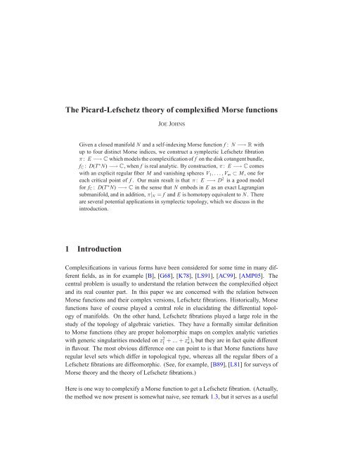
Complexified <strong>Morse</strong> <strong>functions</strong> 7<br />
Figure 1: In the case N = RP 2 , the pieces N0 ,N2 (top), N triv<br />
1 (bottom left), N loc<br />
1 (bottom right).<br />
<strong>The</strong> overlap regions are also indicated.<br />
1.1.2 Sketch <strong>of</strong> the construction <strong>of</strong> N ⊂ E<br />
To construct the required exact Lagrangian embedding N ⊂ E we use a handle-type<br />
decomposition <strong>of</strong> N induced by the <strong>Morse</strong> function f , which is due to Milnor [M65,<br />
pages 27-32]. For example, let us take the usual handle-decomposition <strong>of</strong> N = RP 2<br />
with three handles. <strong>The</strong>n, in the corresponding Milnor decomposition there are four<br />
pieces: First, there are N0 = D 2 and N2 = D 2 , which are the same as the usual 0- and<br />
2-handles. <strong>The</strong>n there is<br />
N loc<br />
1 = {x ∈ R2 : |q2(x)| ≤ 1, |x| 4 − q2(x) 2 ≤ δ},<br />
where δ > 0 is some small number and q2(x) = x 2 1 − x2 2<br />
. Here, Nloc<br />
1<br />
plays the role <strong>of</strong><br />
the 1-handle, but it is diffeomorphic to polygon with eight edges (see figure 1), whereas<br />
a usual 1-handle is diffeomorphic to D 1 × D 1 , which has four edges. For the last piece,<br />
suppose that the 1−handle (in the usual handle-decomposition) is attached using an<br />
embedding<br />
φ: S 0 × [−ǫ,ǫ] −→ S 1 = ∂N0.<br />
<strong>The</strong>n the last piece is<br />
N triv<br />
1 = [S1 \ φ(S 0 × (−ǫ/2,ǫ/2))] × [−1, 1].<br />
This last piece has no analogue in a usual handle-decomposition; roughly, it fills in the<br />
rest <strong>of</strong> the space in N after N0, N2, N loc<br />
1 are glued together. See figure 1 for a picture
8 Joe Johns<br />
<strong>of</strong> the pieces in the Milnor decomposition <strong>of</strong> N = RP 2 .<br />
Now consider the similar case when dim N = 4, and f has three critical points<br />
x0, x2, x4, with <strong>Morse</strong> indices 0, 2, 4. <strong>The</strong>n there is a similar Milnor decomposition<br />
<strong>of</strong> N with, for example, N0 = D4 = N4. To construct N ⊂ E in this case (see §8),<br />
we define several Lagrangian manifolds N0 ⊂ E0, N4 ⊂ E4, Nloc 2 ⊂ E2, Ntriv 2 ⊂ E2<br />
with boundary (with corners) which correspond to exactly to the pieces in the Milnor<br />
decomposition <strong>of</strong> N . Because <strong>of</strong> the way the fibers <strong>of</strong> the Ei are constructed and<br />
the way the Ei are glued together, these Ni glue together exactly as in the Milnor<br />
decomposition <strong>of</strong> N (in particular, with the correct framings). From this it follows that<br />
the union ∪iNi ⊂ E is smooth and diffeomorphic to N .<br />
1.2 Organization<br />
Here is a summary <strong>of</strong> the contents <strong>of</strong> this paper.<br />
§2 We explain some techniques necessary for constructing the regular fiber M and<br />
the vanishing spheres in M. (We only sketch the main ideas in this paper. See<br />
[J09A] for details.) <strong>The</strong> main technique involves attaching <strong>Morse</strong>-Bott type<br />
handles in the Weinstein category. This in turn is related to a generalization <strong>of</strong><br />
Lagrangian surgery to the case where the Lagrangians intersect along any submanifold.<br />
This Lagrangian surgery construction is used to define the vanishing<br />
spheres, and it is also used in the construction <strong>of</strong> M in general.<br />
§3 We explain how to construct the regular fiber M and the vanishing spheres in<br />
M. We discuss the case when f has three or four distinct <strong>Morse</strong> indices in detail,<br />
and we give a partial sketch <strong>of</strong> the general case.<br />
§4 We review some basic constructions for symplectic <strong>Lefschetz</strong> fibrations. Already<br />
in this section we specialize to situations relevant to the case where dim N = 4,<br />
and f has only three distinct <strong>Morse</strong> indices 0, 2, 4.<br />
§5 We construct three <strong>Lefschetz</strong> fibrations πi : Ei −→ D 2 , i = 0, 2, 4 as discussed<br />
sketched in §1.1.1 above.<br />
§6 We construct (E,π) as the fiber connected sum <strong>of</strong> (E0,π0), (E2,π2) (E4,π4), as<br />
sketched in §1.1.1 above.<br />
§7 We check that the vanishing spheres <strong>of</strong> (E,π) with respect to certain vanishing<br />
paths are indeed the expected Lagrangian spheres in M.
Complexified <strong>Morse</strong> <strong>functions</strong> 9<br />
§8 We construct an exact Lagrangian embedding N ⊂ E, as sketched in §1.1.2,<br />
which satisfies the statements in <strong>The</strong>orem A. (See <strong>The</strong>orem 8.1 and Proposition<br />
8.4.)<br />
§9 We look at the case when f : N −→ R has <strong>Morse</strong> indices 0, n, n + 1, 2n + 1,<br />
focusing on the case dim N = 3. We explain the construction <strong>of</strong> (E,π), and<br />
also the construction <strong>of</strong> N ⊂ E.<br />
1.3 Motivations from symplectic topology<br />
In the rest <strong>of</strong> this introduction we will attempt to motivate Problem 1.1, and our proposed<br />
solution <strong>The</strong>orem A, from the point <strong>of</strong> view <strong>of</strong> symplectic topology. <strong>The</strong> most<br />
basic idea is that <strong>Lefschetz</strong> fibrations on a symplectic manifold X give a non-unique<br />
description <strong>of</strong> the total space X in terms <strong>of</strong> a regular hypersurface Y = π −1 (b) and the<br />
vanishing spheres in Y (analogous to a handle-decomposition in differential topology).<br />
Thus, in principle, well-understood <strong>Lefschetz</strong> fibrations for cotangent bundles should<br />
lead to insights about their symplectic topology. For more on this line <strong>of</strong> thought, see<br />
section 1.3.1 below.<br />
A more subtle and surprising fact is that <strong>Lefschetz</strong> fibrations on a symplectic manifold<br />
X can also be used to analyze arbitrary Lagrangian submanifolds L ⊂ X , and<br />
this is the more immediate source <strong>of</strong> our interest in Problem 1.1. <strong>The</strong> original geometric<br />
idea, due to Donalson, is that L ⊂ X should be some kind <strong>of</strong> combination <strong>of</strong><br />
the <strong>Lefschetz</strong> thimbles, obtained by surgery operations. This has only been partially<br />
developed so far in the form <strong>of</strong> matching paths and matching cycles, as in [AMP05],<br />
[S03B], [S08A, §16g]. (See §1.3.2 for the definition and for some plans to develop<br />
this further.) Nevertheless there is a rigorous algebraic version, due to Seidel [S08A,<br />
Corollary 18.25], which is formulated in the Fukaya category <strong>of</strong> X :<br />
(∗) Any L ⊂ X can be expressed as a combination <strong>of</strong> the <strong>Lefschetz</strong> thimbles by<br />
repeatedly forming mapping cones.<br />
Implicitly, this takes place in a context where “mapping cone” makes sense, namely the<br />
so-called derived Fukaya category <strong>of</strong> X . (Conjecturally, mapping cones correspond<br />
to Lagrangian surgery, and so the algebraic and geometric view points should coincide.)<br />
<strong>The</strong>orem A feeds into both <strong>of</strong> these (algebraic and geometric) ideas. First, and foremost,<br />
it provides a good class <strong>of</strong> <strong>Lefschetz</strong> fibrations to be used in combination with<br />
Seidel’s decomposition (∗). In future work we will use this idea to study exact Lagrangian<br />
submanifolds L ⊂ T ∗ N , along the lines <strong>of</strong> [S04] (see §1.3.3 for more on this).
10 Joe Johns<br />
Second, <strong>The</strong>orem A helps to develop Donalson’s original geometric idea, because we<br />
indeed construct N ⊂ E by doing surgery operations among the <strong>Lefschetz</strong> thimbles.<br />
(Actually, while this is essentially true, there is still some work to be done to relate what<br />
we do in this paper to that view point.) Thus the construction <strong>of</strong> N serves as a model<br />
for how to decompose any given Lagrangian L ⊂ E fibering over some path in terms<br />
<strong>of</strong> the <strong>Lefschetz</strong> thimbles. A closely related idea is to define generalized matching<br />
paths for arbitrary manifolds. This involves going in the reverse direction: One starts<br />
with an embedded path γ ⊂ C which passes through several critical values; then,<br />
one constructs a Lagrangian L ⊂ E which fibers over γ , assuming that the <strong>Lefschetz</strong><br />
thimbles lying over γ satisfy suitable matching conditions. We will explore both these<br />
ideas in future work (see 1.3.2 for more details).<br />
Finally, we mention there is a conjecture <strong>of</strong> Seidel [S00, Remark 7.1] which suggests<br />
a way to use <strong>The</strong>orem A, <strong>The</strong>orem B in [J08], and (∗) to relate the two approaches<br />
<strong>of</strong> Fukaya-Seidel-Smith [FSS08, FSS07, S08A] and Nadler-Zaslow [NZ07, N07] for<br />
analyzing the Fukaya category <strong>of</strong> a cotangent bundle (the first approach being <strong>Picard</strong>-<br />
<strong>Lefschetz</strong> <strong>theory</strong>, and the second being comparison with constructible sheaves on N ).<br />
We will not elaborate on this here, but we refer the reader to [J09B] for more on this.<br />
1.3.1 Bifibrations on cotangent bundles<br />
In the most optimistic view, one can start with a <strong>Lefschetz</strong> fibration on T ∗ N (or<br />
any symplectic manifold) and proceding inductively by introducing a new <strong>Lefschetz</strong><br />
fibration on the fiber and, continuing in this way, reduce the symplectic topology <strong>of</strong><br />
the total space to some combinatorial data. This strategy was successfully carried out<br />
very explicitly in the case <strong>of</strong> the quartic surface in [S03B], and then generalized to a<br />
more abstract general setting in [S08A]. In general, one <strong>of</strong>ten has very little detailed<br />
knowledge <strong>of</strong> the <strong>Lefschetz</strong> fibration, and it may be very complicated. For example,<br />
if we are studying a closed symplectic 4-manifold X , the only thing to do in general<br />
is take a Donaldson pencil on X (or maybe a variation on that which maps to CP 2 ).<br />
<strong>The</strong>n, the combinatorial data one gets in this way cannot be reasonably handled, and<br />
in fact basic questions reduce to some hard combinatorial group <strong>theory</strong> problems, as<br />
in [A05]. With this in mind, it is intriguing to start with one <strong>of</strong> our relatively simple<br />
and very explicit <strong>Lefschetz</strong> fibrations π : E −→ D 2 (and let us suppose for simplicity<br />
that E ∼ = D(T ∗ N) as in remark 1.3). <strong>The</strong>n we can ask: Is there a similar <strong>Lefschetz</strong><br />
fibration, say<br />
π2 : M −→ D 2
Complexified <strong>Morse</strong> <strong>functions</strong> 11<br />
defined on the regular fiber? Naively, this seems plausible since M is obtained, roughly<br />
speaking, by plumbing several disk cotangent bundles together (see §3.4), and one<br />
would hope that the model complexifications on each <strong>of</strong> these disk cotangent bundles<br />
can be made to agree on the overlaps, so that they patch together to yield a fibration<br />
on M. (<strong>The</strong> actual construction, though, must combine the fibrations on each disk<br />
cotangent bundle in a more sophisticated way, by combining the regular fibers <strong>of</strong> each<br />
<strong>of</strong> the fibrations into one new regular fiber for the putative fibration on M.) In any case,<br />
once this is known one would like to extend this to the slightly more sophisticated set<br />
up <strong>of</strong> a bifibration on E. Roughly, this is a holomorphic map E −→ C 2 , with generic<br />
singularities, encoding a family <strong>of</strong> <strong>Lefschetz</strong> fibrations on the fibers <strong>of</strong> a <strong>Lefschetz</strong><br />
fibration on E. (For the precise definition, see [S08A, §15e].) As pointed out to me<br />
by Maydanskiy, one potential application <strong>of</strong> such a bifibration (together with work<br />
in progress <strong>of</strong> Seidel) would be to construct exotic cotangent bundles along the same<br />
lines as Maydanskiy’s recent work on exotic sphere cotangent bundles [M09]. More<br />
tentatively, such bifibrations (and similar structures on the fibers <strong>of</strong> π2, etc.) may lead<br />
to interesting matching relations among Lagrangian submanifolds in E, M, etc., in a<br />
spirit similar to [S03B], [S08A]. (See section 1.3.2 below for more about matching<br />
conditions which apply to Lagrangian submanifolds more general than spheres.)<br />
1.3.2 Donaldson’s decomposition and generalized matching paths<br />
Donaldson’s idea is as follows. First, one assumes that π maps L onto an embedded<br />
path γ such that<br />
f = γ −1 ◦ (π|L): L −→ [0, 1]<br />
is a <strong>Morse</strong> function, either by constructing a suitable π for a given L (as achieved<br />
in [AMP05]), or perhaps by deforming the given L and (E,π). <strong>The</strong>n, each critical<br />
point <strong>of</strong> f is a critical point <strong>of</strong> π lying on L, and each unstable and stable manifold<br />
<strong>of</strong> f is part <strong>of</strong> a <strong>Lefschetz</strong> thimble <strong>of</strong> π. <strong>The</strong> expectation is that L is isotopic to a<br />
surgery-theoretic combination <strong>of</strong> all these <strong>Lefschetz</strong> thimbles. This is well-understood<br />
when L is a sphere and γ runs between just two critical values: L is then the union<br />
<strong>of</strong> two <strong>Lefschetz</strong> thimbles meeting at a common vanishing sphere and γ is called a<br />
matching path, see [S08A, §16g], [S03B].<br />
As we mentioned above, the pro<strong>of</strong> <strong>of</strong> <strong>The</strong>orem A involves constructing N ⊂ E by<br />
doing successive surgery operations involving the <strong>Lefschetz</strong> thimbles, just as in Donaldson’s<br />
proposed decomposition. More precisely, let us assume for convenience <strong>of</strong>
12 Joe Johns<br />
notation that f has just one critical point <strong>of</strong> each index. <strong>The</strong>n, we construct a sequence<br />
<strong>of</strong> (not neccesarliy closed) Lagrangian submanifolds N0, N1,...,Nm, where<br />
Nj is diffeomorphic to the jth sublevel set <strong>of</strong> f : N −→ R, i.e. Nj ∼ = {f ≤ cj − ǫ},<br />
where ǫ is small, cj is the jth critical value <strong>of</strong> f , and Nj+1 = Nj#∆j is obtained by a<br />
kind <strong>of</strong> Lagrangian surgery. In future work we will develop two ideas suggested by<br />
this decomposition. First, if L ⊂ E is an arbitrary Lagrangian in the total space <strong>of</strong><br />
an arbitrary <strong>Lefschetz</strong> fibration then the above construction can serve as a model for<br />
how to decompose L as a surgery-theoretic combination <strong>of</strong> the the <strong>Lefschetz</strong> thimbles,<br />
thus making Donalson’s idea more precise. Second, we will formulate the notion <strong>of</strong> a<br />
generalized matching path for arbitrary Lagrangians L.<br />
<strong>The</strong> original notion <strong>of</strong> a mathing path gives a way <strong>of</strong> constructing Lagrangian spheres<br />
in the total space <strong>of</strong> a <strong>Lefschetz</strong> fibration. To do this one assumes there is a path<br />
γ : [0, 1] −→ C joining two critical values c1, c2 such that the two <strong>Lefschetz</strong> thimbles<br />
∆1,∆2 over γ| [0, 1<br />
2 ] and γ| [ 1<br />
2 ,1] have (Lagrangian) isotopic vanishing spheres V1, V2 in<br />
the fiber over γ( 1<br />
2 ) (see [S08A, §16g], or [AMP05, lemma 8.4]). <strong>The</strong> generalization<br />
suggested by our pro<strong>of</strong> <strong>of</strong> <strong>The</strong>orem A is roughly as follows. Take a path γ joining several<br />
critical values c1,...,cm , say γ(tj) = ci, j = 0, 1... , m. <strong>The</strong> simplest matching<br />
condition one could hope for would just involve <strong>Lefschetz</strong> thimbles <strong>of</strong> adjacent pairs<br />
<strong>of</strong> critical points: one would assume that the <strong>Lefschetz</strong> thimbles (up to isotopy) meet<br />
in the expected sphere given by <strong>Morse</strong> <strong>theory</strong>. However, there are important framing<br />
conditions missing here, so the actual matching conditions will be inductive. Let N0<br />
be the the <strong>Lefschetz</strong> thimble <strong>of</strong> c0 , fibered over γ| [t0, 1<br />
(t0+t1)] . For j ≥ 1, assume<br />
2<br />
inductively we have constructed a manifold Nj−1 (built out <strong>of</strong> the <strong>Lefschetz</strong> thimbles<br />
corresponding to c0,...,cj−1 ). <strong>The</strong>n the matching condition will involve Nj−1 and<br />
the <strong>Lefschetz</strong> thimble ∆j at ci which fibers over γ| 1<br />
[ (tj−1+tj),tj] . First, the intersection<br />
2<br />
<strong>of</strong> ∂Nj and ∂∆j in the fiber must be a certain sphere, whose dimension is dictated<br />
by <strong>Morse</strong> <strong>theory</strong>. Second, this sphere will have a framing in ∂Nj which comes from<br />
∆j, and this must also be as dictated by <strong>Morse</strong> <strong>theory</strong>. Roughly, the framing works as<br />
follows. First, take a Weinstein neighborhood D(T∗∆j) ⊂ E. Let Sj denote the sphere<br />
Sj = ∂∆j ∩∂Nj and assume that Sj is bounded by a disk Uj ⊂ ∆j, where ∆j ∼ = Dn and<br />
Uj ∼ = Dk ⊂ Dn . (If we pretend N exists for a moment, then Uj is meant to be ∆j ∩ N ,<br />
which is part <strong>of</strong> the unstable manifold U(xj).) <strong>The</strong>n the k−handle in N corresponding<br />
to xj is represented by the disk conormal bundle<br />
D(ν ∗ Uj) ⊂ D(T ∗ ∆j)<br />
and the framing <strong>of</strong> the handle is encoded in the way D(ν ∗ Uj) meets ∂Nj−1. (Here,<br />
the parameterization ∆j ∼ = D n and the Weinstein embedding D(T ∗ ∆j) ⊂ E should be
Complexified <strong>Morse</strong> <strong>functions</strong> 13<br />
determined to a large degree by a canonical (up to isotopy) parameterization <strong>of</strong> ∂∆j,<br />
as in [S08A, §16b].)<br />
A third point <strong>of</strong> interest is to compare the Donalson and Seidel decompositions. Conjecturally,<br />
the mapping cone <strong>of</strong> a morphism between two Lagrangians L1, L2, let’s say<br />
corresponding to a single point in L1 ∩ L2, say α ∈ CF(L1, L2), is isomorphic to the<br />
Lagrangian surgery <strong>of</strong> L1 and L2, say L1#L2:<br />
Cone(α: L1 → L2) ∼ = L1#L2,<br />
and a version <strong>of</strong> this is known if L1 is a Lagrangian sphere, see [S08A, §17j]. It would<br />
be interesting to prove that Nj+1 = Nj#∆j+1 is isomorphic to Cone(Nj → ∆j+1) in<br />
the above matching path construction. (<strong>The</strong>re is a corresponding result for the case<br />
<strong>of</strong> standard matching paths, [S08A, lemma 18.20].) This would show that whenever<br />
we have a generalized matching path with corresponding Lagrangian L, there is a<br />
Donaldson type decomposition <strong>of</strong> L which coincides with a Seidel decomposition <strong>of</strong><br />
L. Using this together with [AMP05], for example, one might be able to prove a new<br />
version <strong>of</strong> Seidel’s decomposition (∗). This version would rely on choosing different<br />
<strong>Lefschetz</strong> fibrations for different Lagrangians, rather than having one fixed <strong>Lefschetz</strong><br />
fibration.<br />
1.3.3 Lagrangian submanifolds in T ∗ N<br />
Here we elaborate a little on how <strong>The</strong>orem A is relevant for the study <strong>of</strong> exact Lagrangian<br />
submanifolds L ⊂ T ∗ N (see also the introduction to [J09A]). Our basic goal is<br />
to prove for certain N that any closed exact Lagrangian submanifold L ⊂ T ∗ N is Floer<br />
theoretically equivalent to N . This means in particular that HF(L, L) ∼ = HF(N, N), so<br />
N), so that deg(L −→ N) = ±1.<br />
that H∗ (L) ∼ = H∗ (N), and HF(L, T∗ x N) ∼ = HF(N, T∗ x<br />
Of course, results <strong>of</strong> this kind have been obtained for arbitrary manifolds N in<br />
[FSS08, FSS07] and [N07, NZ07]. We want to consider a slightly different approach<br />
along the lines <strong>of</strong> the quiver-theoretic approach for the case N = Sn in [S04]. This approach<br />
avoids spectral sequences and the use <strong>of</strong> gradings; thus it avoids one significant<br />
assumption on L, namely that it has vanishing Maslov class µL ∈ H1 (L).<br />
To keep things concrete, take N = CP 2 , and a <strong>Morse</strong> function f : N −→ R with<br />
three critical points x0, x2, x4 , with <strong>Morse</strong> indices 0, 2, 4. Let (E,π) be the corresponding<br />
<strong>Lefschetz</strong> fibration from <strong>The</strong>orem A, which models the complexification <strong>of</strong> f on<br />
D(T ∗ N). By construction, π comes with an explicit regular fiber M and vanishing<br />
spheres L0, L2, L4 ⊂ M. <strong>The</strong> main consequence <strong>of</strong> <strong>The</strong>orem A is that we have an exact
14 Joe Johns<br />
Lagrangian embedding N ⊂ E. Consequently there is an exact Weinstein embedding<br />
D(T ∗ N) ⊂ E. Now, let L ⊂ T ∗ N be any closed exact Lagrangian submanifold. By<br />
rescaling L ǫL by some small ǫ > 0, we get an exact Lagrangian embedding L ⊂ E.<br />
Now that we know L ⊂ E we can invoke Seidel’s decomposition theorem (∗). Roughly,<br />
it says that we can represent L algebraically (at the level <strong>of</strong> Floer <strong>theory</strong>) in terms <strong>of</strong><br />
the <strong>Lefschetz</strong> thimbles ∆4,∆2,∆0 <strong>of</strong> π. To make this more explicit we need to know<br />
how the <strong>Lefschetz</strong> thimbles interact Floer theoretically. That is, we need to know the<br />
Floer homology groups<br />
(1)<br />
HF(∆4,∆2), HF(∆2,∆0), HF(∆4,∆0),<br />
and also the triangle product (which is defined by counting holomorphic triangles with<br />
boundary on ∆4,∆2,∆0):<br />
(2)<br />
HF(∆4,∆2) ⊗ HF(∆2,∆0) −→ HF(∆4,∆0).<br />
<strong>The</strong>se are precisely the calculations carried out in [J08], except we actually consider<br />
the vanishing spheres Li = ∂∆i ⊂ M, i = 0, 2, 4 and do the corresponding equivalent<br />
calculations in the regular fiber M. (In general, one does not expect to compute things<br />
like (1) and (2) explicitly. It is only because <strong>of</strong> the very explicit and symmetrical nature<br />
<strong>of</strong> M and L0, L2, L4 that the calculations in [J08] can be carried out.)<br />
<strong>The</strong> best way to phrase the answer is to think <strong>of</strong> a category C with three objects<br />
∆4,∆2,∆0 , where the morphisms and compositions are given by (1) and (2). <strong>The</strong>n<br />
<strong>The</strong>orem B in [J08] says that C is given by the following quiver with relations:<br />
(3)<br />
∆4<br />
a1<br />
a0<br />
c1<br />
<br />
∆2<br />
c0<br />
b1<br />
b0<br />
<br />
<br />
∆0<br />
b1a1 = 0, b0a0 = c0, b0a1 − b1a0 = c1<br />
(More precisely, <strong>The</strong>orem B in [J08] says that C is isomorphic to another category,<br />
called the flow category, which is defined entirely in terms <strong>of</strong> the <strong>Morse</strong> <strong>theory</strong> <strong>of</strong><br />
(N, f ); that is where (3) comes from.) <strong>The</strong> upshot <strong>of</strong> Seidel’s decomposition (∗) in this
Complexified <strong>Morse</strong> <strong>functions</strong> 15<br />
case is that L is represented by a certain quiver representation <strong>of</strong> (3):<br />
(4)<br />
W2<br />
A1<br />
A0<br />
C1<br />
<br />
W1<br />
C0<br />
B1<br />
B0<br />
<br />
<br />
W0<br />
B1A1 = 0, B0A0 = C0, B0A1 − B1A0 = C1<br />
Here, the quiver representation (4) is just a choice <strong>of</strong> vector-spaces W4, W2, W0 at each<br />
vertex, and a choice <strong>of</strong> linear maps A0, A1, B0, B1, C0, C1 satisfying the given relations.<br />
To show L is Floer theoretically equivalent to N in T ∗ N is equivalent to showing that<br />
the representation (4) is necessarily isomorphic to the representation<br />
W4 = W2 = W0 = C, A0 = B0 = C0 = id, A1 = B1 = C1 = 0.<br />
(Of course, this is the representation corresponding to N ⊂ T ∗ N .) <strong>The</strong> analogous<br />
problem for N = S n was solved in [S04]. Work on this and related problems is<br />
currently in progress.<br />
Acknowledgements<br />
<strong>The</strong> ideas about matching paths and Donaldson’s decomposition have grown out <strong>of</strong><br />
discussions I had with Denis Auroux a few years ago, while I was in graduate school.<br />
I thank him very much for his hospitality and for generously sharing ideas. <strong>The</strong> ideas<br />
about the nearby Lagrangian conjecture grew out <strong>of</strong> my Ph.D. work with Paul Seidel,<br />
and I thank him warmly as well.<br />
2 <strong>Morse</strong>-Bott handle attachments and Lagrangian surgery<br />
To construct the regular fiber M, we will use an extension <strong>of</strong> Weinstein’s handle attachment<br />
technique where we attach a <strong>Morse</strong>-Bott handle rather than a usual handle.<br />
In this section we only explain the main ideas <strong>of</strong> this construction; for details we refer<br />
the reader to [J09B].<br />
Recall that in [W91] Weinstein explains how to start with a Weinstein manifold<br />
W = W 2n and attach a k−handle D k × D 2n−k , k ≤ n, along an isotropic sphere<br />
in the boundary <strong>of</strong> W to produce a new Weinstein manifold W ′ . (Recall that a Weinstein<br />
manifold is an exact symplectic manifold (W,ω,θ), ω = dθ, equipped with a
16 Joe Johns<br />
Liouville vectorfield X (i.e. one that satisfies ω(X, ·) = θ) such that −X points strictly<br />
inward along the boundary <strong>of</strong> W ; in particular the boundary is <strong>of</strong> contact type.)<br />
In [J09B] we extend this construction to a certain <strong>Morse</strong>-Bott case, namely where<br />
the handle is <strong>of</strong> the form<br />
H = D(T ∗ (S k × D n−k )).<br />
Here we think <strong>of</strong> S k ×{0} ⊂ H as the critical manifold and we think <strong>of</strong> S k ×D n−k ⊂ H<br />
as the unstable manifold <strong>of</strong> S k × {0}. It is not hard to describe how to attach H to W<br />
along the boundary in the smooth category. For that one needs two pieces <strong>of</strong> data:<br />
• a submanifold<br />
S ⊂ ∂W, S ∼ = S k × S n−k−1<br />
(where S now plays the role <strong>of</strong> the attaching sphere), and<br />
• a bundle-isomorphism<br />
T ∗ (S k × D n−k )| (S k ×∂D n−k ) −→ N∂W(S).<br />
Here, N∂W(S) = T(∂W)|S/T(S) is the normal bundle <strong>of</strong> S in ∂W , and the bundle<br />
isomorphism determines a diffeomorphism (up to isotopy) from part <strong>of</strong> the boundary<br />
<strong>of</strong> H to a neighborhood <strong>of</strong> S in ∂W ,<br />
φ: D(T ∗ (S k × D n−k )) (S k ×∂D n−k ) −→ U,<br />
which we use to attach H to W to form W ′ = W ∪ H.<br />
To extend this construction to the Weinstein category, we need only assume that S is<br />
Legendrian in ∂W . <strong>The</strong>n, Weinstein’s construction can be modified so that one starts<br />
with a Weinstein manifold W and produces a new Weinstein manifold W ′ = W ∪ H.<br />
(See [J09B] for details.) <strong>The</strong> main point which is nontrivial is that the boundary <strong>of</strong><br />
W ′ is smooth and convex (i.e. transverse to X ), and in particular <strong>of</strong> contact type. See<br />
figure 3 for a schematic picture <strong>of</strong> W ′ = W ∪ H.<br />
In the usual Weinstein handle attachment, S is an isotropic sphere and the normal<br />
bundle <strong>of</strong> S in ∂W can be decomposed as<br />
N∂W(S) ∼ = τ 1 S ⊕ T∗ S ⊕ TS ω /TS,<br />
where τ 1 S is the trivial real line bundle over S, and TSω is the symplectic orthogonal<br />
complement in T(∂W)). Thus the first two terms necessarily sum to a trivial bundle,<br />
and the only part which is possibly nontrivial is TS ω /TS (denoted CSN(S) in [W91]).
Complexified <strong>Morse</strong> <strong>functions</strong> 17<br />
In our case, one has the same splitting<br />
(5)<br />
N∂W(S) ∼ = τ 1 S ⊕ T∗ S ⊕ TS ω /TS,<br />
but, since S is Legendrian, we have TS ω /TS = 0. On the other hand S ∼ = S k × S n−k−1<br />
is not a sphere, so<br />
τ 1 S ⊕ T∗ S ∼ = τ 1 S ⊕ T∗ S k × T ∗ S n−k−1<br />
is usually not trivial. (Here T ∗ S k × T ∗ S n−k−1 −→ S k × S n−k−1 is just the Cartesian<br />
product <strong>of</strong> the total spaces.) <strong>The</strong>re is, however, a canonical isomorphism<br />
(6)<br />
τ 1 S ⊕ T ∗ S ∼ = T ∗ (S k × D n−k )| S k ×∂D n−k.<br />
So, for us, we do not need to choose any framing data; we only need to choose the<br />
identification S ∼ = S k × S n−k . See §2.1 below for how this identification is chosen in<br />
some special situations.<br />
Note that we have only extended the Weinstein construction to a very particular <strong>Morse</strong>-<br />
Bott situation, namely the case where the critical manifold C is a sphere, and the<br />
normal bundle <strong>of</strong> C has a certain form. In general, a <strong>Morse</strong>-Bott function f : X −→ R<br />
can have an arbitrary connected manifold C as critical manifold, and the normal bundle<br />
<strong>of</strong> C in X , say E −→ C, can be arbitrary. In that situation the <strong>Morse</strong>-Bott handle<br />
would be modeled on the bundle D(E+) × D(E−) −→ C, with fiber D k × D n−k , where<br />
E ∼ = E+ ⊕E− is the splitting <strong>of</strong> E into positive and negative eigenspaces <strong>of</strong> the Hessian<br />
<strong>of</strong> f at C. It might be interesting to extend the Weinstein construction to the general<br />
<strong>Morse</strong>-Bott case.<br />
2.1 How this construction is applied<br />
When we construct the regular fiber M in various cases (see §3) we will repeatedly<br />
apply the above handle-attachment construction in the following set up. We take<br />
W = D(T ∗ L),<br />
i.e. the disk bundle cotangent bundle <strong>of</strong> some manifold L = L n , with respect to some<br />
metric on T ∗ L. <strong>The</strong>n we take an embedded sphere<br />
S n−k−1 ⊂ L<br />
with a chosen parameterization <strong>of</strong> tubular neighborhood <strong>of</strong> S n−k−1 ⊂ L,<br />
(7)<br />
φ: S n−k−1 × D k+1 −→ L
18 Joe Johns<br />
corresponding to a chosen trivialization <strong>of</strong> the normal bundle <strong>of</strong> S n−k−1 in L. (This<br />
trivialization will be part <strong>of</strong> the framing data in a chosen handle decomposition <strong>of</strong> our<br />
manifold N corresponding to the <strong>Morse</strong> function f : N −→ R; L will correspond to<br />
a regular level set <strong>of</strong> f and S n−k−1 will be an attaching sphere; see §3.4.) Thus the<br />
conormal bundle<br />
ν ∗ S n−k−1 ⊂ T ∗ L<br />
is trivial; we take S ⊂ ∂W to be the sphere bundle<br />
S = S(ν ∗ S n−k−1 ) ∼ = S n−k−1 × S k<br />
with a corresponding trivialization S ∼ = S n−k−1 × S k determined by the chosen framing<br />
(7). Of course S is Legendrian in ∂W = S(T ∗ L) since ν ∗ S n−k−1 is Lagrangian in T ∗ L.<br />
<strong>The</strong> bundle isomorphism<br />
T ∗ (S k × D n−k )| S k ×∂D n−k ) −→ N∂W(S)<br />
is determined by (5) and (6), since S Legendrian implies TS ω /TS = 0.<br />
2.2 Lagrangian surgery<br />
One special property possessed by the Weinstein manifold<br />
W ′ = D(T ∗ N) ∪ H<br />
is the existence <strong>of</strong> an exact Lagrangian sphere Z ⊂ W ′ . Namely, Z is the union <strong>of</strong> the<br />
disk conormal bundle D(ν ∗ S n−k−1 ) and the unstable manifold S k × D n−k ⊂ H:<br />
Maybe it is helpful to identify<br />
Z = D(ν ∗ S n−k−1 ) ∪ (S k × D n−k ) ⊂ D(T ∗ N) ∪ H.<br />
Z = {(u1,... , un+1) ∈ R n+1 : Σiu 2 i = 1};<br />
then, one can think <strong>of</strong> S k × D n−k ⊂ H and D(ν ∗ S n−k−1 ) ⊂ D(T ∗ L) as corresponding<br />
to overlapping neighborhoods <strong>of</strong> the two subspheres<br />
K+ = {(u1,...,uk+1, 0,... , 0) ∈ R n+1 : Σiu 2 i = 1}, and<br />
K− = {(0,... , 0, uk+2,... , un+1) ∈ R n+1 : Σiu 2 i<br />
= 1}.<br />
Z is smooth because the two pieces can be made to overlap smoothly; it is Lagrangian<br />
since each piece is Lagrangian; and it is exact because each piece is exact, and the<br />
overlap region is connected.
Complexified <strong>Morse</strong> <strong>functions</strong> 19<br />
A more interesting fact is that W ′ contains a Lagrangian submanifold<br />
L ′ ⊂ W ′<br />
which is diffeomorphic to the result <strong>of</strong> doing surgery on L along the framed sphere<br />
S n−k−1 ⊂ L (where the framing is (7)). This construction is used to define the Lagrangian<br />
vanishing spheres in M, see §3. It is also used in the construction <strong>of</strong> M in the<br />
general case, see §3.4. One can think <strong>of</strong> L ′ as the Lagrangian surgery <strong>of</strong> L and Z along<br />
S n−k−1 . (This construction can be generalized to the case <strong>of</strong> any two Lagrangians<br />
meeting cleanly along a connected closed manifold C ⊂ L1, L2, where C has trivial<br />
normal bundle in L1 and L2, see [J09B].)<br />
To define L ′ we start with an exact Weinstein embedding for Z ⊂ W ′<br />
φZ : Dr(T ∗ S n ) −→ W ′ ,<br />
where Dr(T ∗ S n ) is the disk bundle with respect to the round metric <strong>of</strong> some suitably<br />
small radius r > 0. Let us realize T ∗ S n as the following exact symplectic submanifold<br />
<strong>of</strong> R 2n+2 :<br />
(8)<br />
T ∗ S n = {(u, v) ∈ R n+1 × R n+1 : |u| = 1, u · v = 0}.<br />
<strong>The</strong>n, the subsphere K− ⊂ S n we defined above has an obvious identification <strong>of</strong> its<br />
conormal bundle with S n−k−1 × R k+1 , because<br />
ν ∗ K− = {((0,... , 0, uk+2,... , un+1), (v1,... , vk+1, 0... , 0)) ∈ R n+1 ×R n+1 : Σiu 2 i = 1}.<br />
And <strong>of</strong> course there is a similar identification for K+,<br />
ν ∗ K+ ∼ = S k × R n−k .<br />
Now assume that φZ maps Dr(ν ∗ K−) onto a neighborhood <strong>of</strong> S n−k−1 ⊂ L. In fact we<br />
may assume φZ|Dr(ν ∗ K−) agrees with the previously chosen framing (7):<br />
(9)<br />
φZ|Dr(ν ∗ K−) = φ| S n−k−1 ×D k+1<br />
r<br />
: S n−k−1 × D k+1<br />
r<br />
−→ L,<br />
where we are using the canonical identification Dr(ν ∗K−) ∼ = Sn−k−1 × Dk+1 r . (To see<br />
why we can assume (9), see the embedding (13) below; we can take our Weinstein<br />
embedding φZ to be the restriction <strong>of</strong> that. Alternatively, one can invoke Pozniack’s<br />
local model for cleanly intersecting Lagrangians [P94, Proposition 3.4.1].)<br />
2.2.1 Construction <strong>of</strong> L ′ up to homeomorphism (denoted L ′ )<br />
To see the rough idea for the construction <strong>of</strong> L ′ , let us assume for convenience that r = 1<br />
for a moment. Now let Φ denote the time π/2 geodesic flow on D(T ∗ S n ) = D1(T ∗ S n )
20 Joe Johns<br />
Figure 2: Consider the low-dimensional situation D(T ∗ Z) ∼ = D1(T ∗ S 1 ), K+, K− ∼ = S 0 . We<br />
have depicted D1(T ∗ S 1 ) as R/2πZ×[−1, 1]. <strong>The</strong> horizontal green line represents Z ∼ = R/2πZ;<br />
the two vertical blue lines represent D(ν ∗ K−) ∼ = S 0 × [−1, 1]; and the two curved red lines<br />
represent T = Φ(D(ν ∗ K+)).<br />
(which is Hamiltonian). <strong>The</strong> effect <strong>of</strong> Φ on D(ν ∗ K+) is to fix vectors <strong>of</strong> zero length<br />
(i.e. points in K+) and map the unit vectors S(T ∗ K+) diffeomorphically onto S(T ∗ K−),<br />
while vectors <strong>of</strong> intermediate length interpolate between these extremes. (See figure<br />
2 for the case when dim D(T ∗ Z) = 2 and Φ is tweaked slightly to Φ.) Up to<br />
homeomorphism, L ′ can be described as follows: Define<br />
and set<br />
T<br />
T = Φ(D(ν ∗ K+))<br />
L ′ = (L \ φZ(D(ν ∗ K−))) ∪ φZ(T).<br />
<strong>The</strong>n it is clear that L ′ is homeomorphic to the surgery <strong>of</strong> L along the framed sphere<br />
S n−k−1 = φZ(K−), where the framing is given by (9).<br />
<strong>The</strong> only problem is that L ′ is not smooth, because T is not tangent to D(ν ∗ K−) along<br />
∂D(ν ∗ K−). To fix this, we just need to tweak Φ slightly to get a new Hamiltonian<br />
diffeomorphism Φ such that T = Φ(D(ν ∗ K+)) agrees with D(ν ∗ K−) in a neighborhood<br />
<strong>of</strong> ∂D(ν ∗ K−). <strong>The</strong>n L ′ = (L \ φZ(D(ν ∗ K−))) ∪ φZ(T) will be smooth. (See<br />
figure 2 for a picture <strong>of</strong> the low dimensional situation: D(T ∗ Z) ∼ = D(T ∗ S n ) = D(T ∗ S 1 ),<br />
K−, K+ ∼ = S 0 .) We spell the details out now since we will need them available later.<br />
2.2.2 Construction <strong>of</strong> L ′ as a smooth Lagrangian submanifold<br />
First, consider the normalized geodesic flow on T ∗ S n \S n , which moves each (co)vector<br />
at unit speed for time t, regardless <strong>of</strong> its length. This has an explicit formula in terms
Complexified <strong>Morse</strong> <strong>functions</strong> 21<br />
<strong>of</strong> the coordinates (8):<br />
σt : T ∗ S n \ S n −→ T ∗ S n \ S n ,σt(u, v) = (cos tu + sin t v v<br />
, cos t − sin tu).<br />
|v| |v|<br />
Given any function H : T ∗ S 3 \ S 3 −→ R we let φ H t denote the time t Hamiltonian<br />
flow <strong>of</strong> XH (our convention is ω(·, XH) = dH). It is elementary to check that for any<br />
k ∈ C ∞ (R, R),<br />
(10)<br />
Let<br />
<strong>The</strong>n it is well-known that φ (1/2)µ2<br />
t<br />
φ k(H)<br />
t (p) = φ H k ′ (H(p))t (p).<br />
µ: T ∗ S 3 \ S 3 −→ R,µ(u, v) = |v|.<br />
is the usual geodesic flow and so (10) implies<br />
φ µ t is equal to the normalized geodesic flow, with the formula given by σt . Now let<br />
h: R −→ R be any smooth function satisfying<br />
(11)<br />
h ′ (0) = 0,<br />
h ′ (t) = 1/2, t ∈ [r/2, r],<br />
h ′′ (t) > 0, t ∈ [0, r/2),<br />
h(−t) = h(t) − t for small |t|<br />
In §5.1 we will make a particular choice for h. Consider the map<br />
defined by<br />
F : Dr(T ∗ S 3 ) \ S 3 −→ Dr(T ∗ S 3 ) \ S 3<br />
F(u, v) = φ h(µ)<br />
π/2 (u, v) = σ h ′ (|v|)π(u, v).<br />
<strong>The</strong>n F extends continuously over the zero-section because h ′ (0) = 0. To see that<br />
the extension is smooth one applies [S03A, Lemma 1.8]. (This is why we need<br />
h(−t) = h(t) − t for small |t|.) Call the extension<br />
F : Dr(T ∗ S 3 ) −→ Dr(T ∗ S 3 ).<br />
(Here, F plays the role <strong>of</strong> Φ before.) Now define<br />
Notice that<br />
T = F(Dr(ν ∗ K+)).<br />
F(D [r/2,r](ν ∗ K+)) = D [r/2,r](ν ∗ K−).<br />
(One can see this by the formula for σ π/2 .) It follows that<br />
(12)<br />
T ∩ Dr(ν ∗ K−) = D [r/2,r](ν ∗ K−).
22 Joe Johns<br />
(This is an equality rather than just containment because h ′′ (t) > 0, t ∈ [0, r/2).) Now<br />
set<br />
L ′ = (L \ φZ(D r/2(ν ∗ K−))) ∪ φZ(T).<br />
<strong>The</strong>n L ′ is smooth because there is an overlap<br />
[L \ φZ(D r/2(ν ∗ K−))] ∩ φZ(T) = φZ(D (r/2,r](ν ∗ K−)),<br />
because <strong>of</strong> (12). L ′ is Lagrangian because T and [L \ φZ(D r/2(ν ∗ K−))] are, and<br />
the overlap has nonempty interior in L. Since F Hamiltonian implies T is exact,<br />
it follows that if L is exact and the overlap region between L and φZ(T) (namely<br />
φZ(D [r/2,r](ν ∗ K−)) ∼ = S n−k−1 × D k+1<br />
[r/2,r] , n ≥ 1, k ≥ 0) is connected then L′ will be<br />
exact as well.<br />
2.3 Plumbing<br />
<strong>The</strong>re is an alternative construction called symplectic plumbing, which (in particular)<br />
produces a manifold W 0 homeomorphic to W ′ = D(T ∗ N) ∪ H from the last section.<br />
We do not use this construction in this paper (mainly because the boundary <strong>of</strong> W 0 is<br />
not smooth), but it gives a useful alternative view point, and it is used in [J08], so we<br />
discuss it briefly here. From time to time we may mention it to give some additional<br />
clarification in visualizing things.<br />
Take two disk cotangent bundles D(T ∗ L1) and D(T ∗ L2) and assume that there is a<br />
closed manifold K (connected, say) which has embeddings<br />
K ⊂ L1, and K ⊂ L2.<br />
Assume moreover that the normal bundle <strong>of</strong> K in both L1 and L2 is trivial and choose<br />
tubular neighborhoods<br />
where dim Li = n, dim K = k.<br />
K × D n−k ⊂ L1, and K × D n−k ⊂ L2,<br />
<strong>The</strong> idea <strong>of</strong> the symplectic plumbing construction is to glue D(T ∗ L1) and D(T ∗ L3)<br />
together along neighborhoods <strong>of</strong> K ⊂ D(T ∗ L1) and K ⊂ D(T ∗ L2), so that the intersection<br />
<strong>of</strong> L1 and L2 is precisely K , and the intersection is clean, or <strong>Morse</strong>-Bott, i.e.<br />
T(L1) ∩ T(L2) = T(K).<br />
More precisely, the submanifolds K × D n−k ⊂ L1, L2 have tubular neighborhoods<br />
W1 ⊂ D(T ∗ L1), W2 ⊂ D(T ∗ L2),
Complexified <strong>Morse</strong> <strong>functions</strong> 23<br />
L<br />
Z<br />
Figure 3: Schematic <strong>of</strong> W 0 = D(T ∗ L) ⊞ D(T ∗ S n ) embedded into W ′ = D(T ∗ L) ∪ H near<br />
plumbing or handle-attachment region. Parts <strong>of</strong> L and the Lagrangian sphere Z are also labeled.<br />
with exact symplectomorphisms<br />
W1, W2 ∼ = D(T ∗ (K × D n−k )).<br />
(Here, we assume that S(T ∗ (K × D n−k )) ⊂ S(T ∗ Li), i = 1, 2.) To define the plumbing<br />
W 0 = D(T ∗ L1) ⊞ D(T ∗ L2)<br />
we take the quotient <strong>of</strong> the disjoint union D(T ∗ L1) ⊔ D(T ∗ L2), where we identify W1<br />
and W2 using a suitable exact symplectomorphism<br />
η : D(T ∗ (K × D n−k )) −→ D(T ∗ (K × D n−k ))<br />
which sends K × D n−k to D(ν ∗ K) and D(ν ∗ K) to K × D n−k . This means that in W 0<br />
a tubular neighborhood <strong>of</strong> K in L1 is identified with the disk conormal bundle <strong>of</strong> K<br />
in D(T ∗ L2), and vice-versa. (This condition is motivated by Pozniack’s local model<br />
[P94, Proposition 3.4.1].)<br />
To define η, let us pass for a moment to the noncompact model<br />
T ∗ (K × R n−k ) ∼ = T ∗ K × T ∗ R n−k ∼ = T ∗ K × C n−k .
24 Joe Johns<br />
It is easy to see that ν ∗ K ⊂ T ∗ (K × R n−k ) corresponds to K × i R n−k ⊂ T ∗ K × C n−k<br />
in this model. Thus, we can η to be the restriction <strong>of</strong> the map<br />
idT ∗ K × m(i): T ∗ K × C n−k −→ T ∗ K × C n−k .<br />
<strong>The</strong>re is one sticky point, which is that W1 and W2 correspond to subsets <strong>of</strong> T ∗ K×C n−k<br />
with boundary (with corners), and so one has to be a little bit careful to choose the disk<br />
bundles D(T ∗ L1) and D(T ∗ L2) so that these boundaries correspond nicely under the<br />
map idT ∗ K × m(i). (See [J09B] for details.)<br />
To relate this to the handle attachment W ′ = D(T ∗ L) ∪ H we take L1 = L to be<br />
any manifold and K = S n−k−1 ⊂ L with the chosen framing S n−k−1 × D k+1 ⊂ L as in<br />
§2.1. <strong>The</strong>n we we take<br />
L2 = S n = {(u1,...,un+1) ∈ R n+1 : Σu 2 i<br />
= 1},<br />
and we take S n−k−1 = K− ⊂ L2 as in §2.2 with the the obvious canonical framing<br />
S n−k−1 × D k+1 ⊂ L2. <strong>The</strong>n,<br />
is homeomorphic to<br />
W 0 = D(T ∗ L) ⊞ D(T ∗ S n )<br />
W ′ = D(T ∗ L) ∪ H.<br />
Moreover, there is an exact symplectic embedding<br />
(13)<br />
ρ: D(T ∗ L) ⊞ D(T ∗ S n ) −→ D(T ∗ L) ∪ H<br />
such that ρ|L = idL and ρ(S n ) = Z (see figure 3). See [J09B] for the pro<strong>of</strong>.<br />
3 Construction <strong>of</strong> the regular fiber M and the Lagrangian<br />
vanishing spheres<br />
Let N be a closed manifold and let f : N −→ R be self-indexing <strong>Morse</strong> function. In<br />
this section we will explain how to construct the regular fiber M and the Lagrangian<br />
vanishing spheres L1,...,Lm ⊂ M for π : E −→ D 2 .<br />
We will deal with three cases:<br />
(1) f has three distinct <strong>Morse</strong> indices 0, n, 2n (see §3.1 and 3.2).<br />
(2) f has four distinct <strong>Morse</strong> indices 0, n, n + 1, 2n + 1 (see §3.3).<br />
(3) <strong>The</strong> general case (partial sketch- see §3.4).
Complexified <strong>Morse</strong> <strong>functions</strong> 25<br />
<strong>The</strong> construction <strong>of</strong> M in each case is identical as the dimension <strong>of</strong> N varies. For<br />
this reason we will keep things slightly more concrete in the first two cases above by<br />
focusing on the cases when dim N = 4 and dim N = 3 respectively. See §3.2 for<br />
how things work in an arbitrary dimension in case (1).<br />
3.1 Constructing M and the vanishing spheres in case (1), dim N = 4<br />
Suppose N is a closed 4-manifold and<br />
f : N −→ R<br />
has critical points x0, x j<br />
2 , x4, j = 1,... , k, where the subscript indicates the <strong>Morse</strong><br />
index. Let g be a Riemannian metric such that (f, g) is <strong>Morse</strong>-Smale.<br />
First, (f, g) induces a handle decomposition <strong>of</strong> N , which determines k framed knots<br />
Kj ⊂ S 3 , which are the attaching spheres <strong>of</strong> the 2-handles, together with a parameterization<br />
<strong>of</strong> a tubular neighborhood <strong>of</strong> each Kj<br />
(14)<br />
φj : S 1 × D 2 −→ S 3 ,<br />
determined by the framing for the 2-handle up to isotopy. Set<br />
L0 = S 3 .<br />
We start with the disk bundle D(T ∗ L0). To construct M, we attach a <strong>Morse</strong>-Bott handle<br />
Hj = D(T ∗ (S 1 × D 2 ))<br />
to D(T ∗ L0) for each j, where the gluing region is a neighborhood <strong>of</strong> S(ν ∗ Kj) in S(T ∗ L0),<br />
and the framing φj determines the gluing map. This produces a Weinstein manifold<br />
M = D(T ∗ L0) ∪ (∪jHj),<br />
as we explained in §2.1. We have for each j an exact Lagrangian 3-sphere<br />
L j<br />
2 ⊂ M<br />
which is the union <strong>of</strong> D(ν∗Kj) and S1 × D2 ⊂ Hj. (Each L j<br />
2 corresponds to what we<br />
called Z in §2.2.) See figure 3 in §2.3 for a schematic picture <strong>of</strong> the region near each<br />
attaching region.<br />
Now define L4 as the Lagrangian surgery <strong>of</strong> L0 and all the L j<br />
2 ’s. In §2.2 we explain<br />
how to define the Lagrangian surgery <strong>of</strong> L ⊂ D(T∗L) ∪ H and a single Lagrangian<br />
’s simultaneously, where<br />
sphere Z ⊂ D(T ∗ L) ∪ H. We use that definition for all L j<br />
2
26 Joe Johns<br />
each L j<br />
2 plays the role <strong>of</strong> Z . L4 is exact since it is simply-connected. Thus we have<br />
defined exact Lagrangian spheres L0, L j<br />
2 , L4 in M, one for each critical point x0, x j<br />
2 , x4<br />
<strong>of</strong> f . If dim N = 2 then there is an analogous construction <strong>of</strong> a 2 dimensional version<br />
<strong>of</strong> M; see figure 7 in §5.4 for the case when f has four critical points with <strong>Morse</strong><br />
indices 0,1,1,2.<br />
<strong>The</strong>re is one ingredient in the surgery construction which is useful to record here.<br />
⊂ M,<br />
Namely, we must fix exact Weinstein embeddings for each L j<br />
2<br />
φ j<br />
L : Dr(T<br />
2<br />
∗ S 3 ) −→ M,<br />
where Dr(T ∗S3 ) is the disk bundle with respect to the round metric <strong>of</strong> radius r > 0.<br />
φ j should also agree with the framing (14) along Dr(ν L2 ∗K−), that is, we assume<br />
φ j|Dr(ν<br />
L2 ∗K−) : Dr(ν ∗ K−) −→ L0<br />
coincides with<br />
φj| S 1 ×D 2 r : S 1 × D 2 r −→ S 3 .<br />
Remark 3.1 In the case dim N = 2 one can show that the analogue <strong>of</strong> L4 (which<br />
would be L2 corresponding to a critical point <strong>of</strong> index 2) is exact by applying lemma<br />
is exact and τ is exact. <strong>The</strong> analogous<br />
7.2. That lemma says L4 = τ(L ′ 4 ) where L′ 4<br />
lemma in the case dim N = 2 says L2 = τ(L ′ 2 ).<br />
3.2 Constructing M and the vanishing spheres in case (1), dim N = 2n<br />
In this section we quickly sketch how the construction works in the more general case<br />
where dim N = 2n and the <strong>Morse</strong> indices <strong>of</strong> f are 0, n, 2n; it is much the same as §3.1.<br />
In this case the handle-decomposition <strong>of</strong> N corresponding to (f, g) determines k<br />
attaching spheres<br />
Kj ⊂ S 2n−1 , Kj ∼ = S n−1<br />
with framings<br />
φj : S n−1 × D n −→ S 2n−1 .<br />
To construct M, we set L0 = S n−1 and then attach k <strong>Morse</strong>-Bott handles<br />
Hj ∼ = D(T ∗ (S n−1 × D n ))<br />
to D(T ∗ L0) where the attaching region is a neighborhood <strong>of</strong> S(ν ∗ Kj) ⊂ S(T ∗ L0), and<br />
the attaching maps are determined by framings φj . <strong>The</strong> other vanishing cycles L j n, L2n<br />
are defined as before.
Complexified <strong>Morse</strong> <strong>functions</strong> 27<br />
3.3 Constructing M and the vanishing spheres in case (2), dim N = 3<br />
In this section we explain how, for a closed 3-manifold N , one can construct the<br />
regular fiber M and vanishing spheres L0, L1, L2, L3 in M. This discussion applies<br />
equally well to self-indexing <strong>Morse</strong> <strong>functions</strong> f : N −→ R with four critical values<br />
0, n, n + 1, 2n + 1. See section 3.2 to see how things are much the same from one<br />
dimension to the next.<br />
Let (N, f, g) be a triple consisting <strong>of</strong> a closed 3-manifold N , and a self-indexing<br />
<strong>Morse</strong> function f : N −→ R, together with a <strong>Morse</strong>-Smale metric g on N . <strong>The</strong>n<br />
(N, f, g) determines a Heegard diagram for N as follows. Let<br />
T = f −1 (3/2).<br />
This is a closed 2-manifold <strong>of</strong> some genus h. We may assume f has h critical points<br />
, j = 1,... , h. <strong>The</strong>n there are h circles<br />
<strong>of</strong> index 1 and 2, x j j<br />
1 , x2 namely<br />
where S(x j<br />
1<br />
αj,βj ⊂ T, j = 1,... g,<br />
αj = S(x j<br />
) is the stable manifold <strong>of</strong> x j<br />
1<br />
1 ) ∩ T,βj = U(x j<br />
2 ) ∩ T,<br />
and U(x j<br />
1<br />
) is the unstable manifold <strong>of</strong> x j<br />
1 .<br />
<strong>The</strong> data <strong>of</strong> T together with the circles αj,βj is called a Heegard diagram for N ; it<br />
determines the diffeomorphism type <strong>of</strong> N . In addition, (f, g) determine framings<br />
φ α j : S1 × D 1 −→ T<br />
φ β<br />
j : S1 × D 1 −→ T<br />
for αj , βj respectively. (Of course, in this dimension, there are only two possible<br />
framings for each αj or βj and they give rise to diffeomorphic manifolds. But in higher<br />
dimensions the analogue <strong>of</strong> these framings are important.)<br />
<strong>The</strong>n M is defined as follows. Set<br />
L j j<br />
1 , L2 = S2 , j = 1,... , h.<br />
Now consider the disk bundle D(T ∗ T) and consider the disk conormal bundles D(ν ∗ (αj))<br />
and D(ν ∗ (βj)), each being diffeomorphic to S 1 × D 1 . Since (f, g) is <strong>Morse</strong>-Smale, it<br />
follows that αj and βk are transverse for any j, k. <strong>The</strong>refore we may assume that the<br />
boundaries <strong>of</strong> the disk conormal bundles S(ν ∗ (αj)) and S(ν ∗ (βk)) are disjoint for every
28 Joe Johns<br />
Figure 4: <strong>The</strong> case N = S 3 , where f has four critical points <strong>of</strong> index 0,1,2,3. This is a<br />
schematic <strong>of</strong> M, depicting T = T 2 , with one α curve and one β curve, together with two<br />
vanishing spheres, L1 and L2 which meet T at α and β . <strong>The</strong> other two vanishing spheres L0<br />
and L2 are not depicted; they are obtained as the surgery <strong>of</strong> T and L1 , respectively T and L2 .<br />
(<strong>The</strong> caption <strong>of</strong> figure 5 attempts to describe how to visualize L0 and L3 .)<br />
j, k. This means we can attach handles to D(T ∗ T) along S(ν ∗ (αj)) and SR(ν ∗ (βk)) as<br />
follows. Take 2h <strong>Morse</strong>-Bott handles<br />
H α j = D(T∗ (S 0 × D 2 ))<br />
H β<br />
j = D(T∗ (S 0 × D 2 )).<br />
(Note that, when dim N = 3 as in our case, each D(T∗ (S0 × D2 )) is just the disjoint<br />
union <strong>of</strong> two usual (not <strong>Morse</strong>-Bott) 2−handles D(T∗D2 ).) To construct M we attach<br />
each Hα j and Hβ j to the boundary <strong>of</strong> D(T∗T) in such a way that the core <strong>of</strong> Hα j , that<br />
is S0 × D2 , is glued to D(ν∗ (αj)) along their boundaries, and similarly for H β<br />
j and<br />
D(ν∗ (βj)). Thus the union <strong>of</strong> the core <strong>of</strong> Hα j , given by S0 × D2 , and D(ν∗αj)) forms<br />
an exact Lagrangian 2-sphere<br />
L j<br />
1 ⊂ M<br />
which intersects T in αj , and similarly we have<br />
which intersects T in βj . Here, L j<br />
1<br />
L j<br />
2 ⊂ M<br />
j<br />
, L2 are analogous to Z in §2.2. (If one is not<br />
concerned about M having a smooth boundary, one can alternatively define M as the<br />
plumbing (see §2.3) <strong>of</strong> DR(T ∗ T) and Dr(T ∗ L j<br />
1 ) along αj and Dr(T ∗ L j<br />
2 ) along βj, for
Complexified <strong>Morse</strong> <strong>functions</strong> 29<br />
01<br />
01<br />
Figure 5: A two dimensional vanishing sphere (relevant for dim N = 3). Depicted schematically<br />
are the (disk) conormal bundles <strong>of</strong> K+ = S 0 and K− = S 1 . To visualize the surgery<br />
<strong>of</strong> T and L1 , say, first imagine bending the conormal bundle <strong>of</strong> K+ so that its two boundary<br />
circles are identified with the two boundary circles <strong>of</strong> the conormal bundle <strong>of</strong> K− . (Formally<br />
speaking, this “bending” is done by reparameterized geodesic flow.) Second, imagine that the<br />
conormal bundle <strong>of</strong> K− is identified with a neighborhood <strong>of</strong> the α curve in T , say N(α) (see<br />
figure 4). Thus, the union <strong>of</strong> the bent conormal bundle <strong>of</strong> K+ and T \ N(α) together form a<br />
2-sphere which is L0 .<br />
some 0 < r < R.) <strong>The</strong> precise attaching maps for H α j<br />
framings φ α j<br />
and φβj<br />
. Let<br />
and Hβ<br />
j<br />
K− = {(u1, u2, 0) : Σju 2 j = 1} ⊂ S 2<br />
K+ = {(0, 0, u3) : u3 = ±1} ⊂ S 2 .<br />
<strong>The</strong>re are exact Weinstein embeddings <strong>of</strong> L j j<br />
2 and L1 ,<br />
such that<br />
and<br />
φ j : Dr(T L2 ∗ S 3 ) −→ M<br />
φ j : Dr(T L1 ∗ S 3 ) −→ M,<br />
φ j<br />
L (K−) = αj<br />
1<br />
φ j<br />
L (K−) = βj<br />
2<br />
φ j<br />
1 |Dr(ν ∗ K−) = φ α j<br />
φ j<br />
2 |Dr(ν ∗ K−) = φ β<br />
j .<br />
are determined by the
30 Joe Johns<br />
Here T ∗ L j<br />
1 , T∗ L j<br />
2 are equipped with the standard round metric <strong>of</strong> T∗ S 2 . We define L0<br />
as the Lagrangian surgery <strong>of</strong> T and the L j<br />
1<br />
parts to L0: one is T \ (∪jφ α j (S1 × D 1 r/2<br />
’s, as in §2.2. More precisely, there are two<br />
)), and the other is the union <strong>of</strong> some subsets<br />
<strong>of</strong> φ j<br />
L (Dr(T<br />
1<br />
∗S2 )) which are defined by taking Dr(ν ∗K+) ∼ = S0 × D2 and applying a<br />
reparameterized geodesic flow map to it. L3 is defined similarly: it is the surgery <strong>of</strong><br />
T and the L j<br />
2 ’s. See figure 4 for a schematic <strong>of</strong> M, and figure 5 for a schematic <strong>of</strong> a<br />
vanishing sphere to help with visualizing surgery.<br />
3.4 Partial sketch <strong>of</strong> the construction <strong>of</strong> M for arbitrary <strong>Morse</strong> <strong>functions</strong>.<br />
Let N be a closed manifold <strong>of</strong> dimension n. Assume for simplicity <strong>of</strong> notation that<br />
f : N −→ R is self-indexing with just one critical point <strong>of</strong> each index i0, i1,... , ik .<br />
As a starting motivation, we expect to have one Lagrangian sphere Lj in M for each<br />
<strong>of</strong> f . Secondly, in M we expect to find that each regular level set <strong>of</strong><br />
critical point xij<br />
f in N is embedded as a Lagrangian submanifold in M. This is because in the total<br />
space <strong>of</strong> the <strong>Lefschetz</strong> fibration fC : D(T∗L0) −→ C the real level set f −1 (ij ± ǫ) is<br />
obviously Lagrangian in the complex level set f −1<br />
C (ij ± ǫ); but then we can transport<br />
all <strong>of</strong> these Lagrangians into one common fixed regular fiber <strong>of</strong> fC.<br />
Here then is the rough idea for the construction <strong>of</strong> M. Take D(T ∗ L0), . . . , D(T ∗ Lk),<br />
one for each critical point <strong>of</strong> f : N −→ R. We take a handle-decomposition <strong>of</strong> N<br />
corresponding to f (and some fixed metric g such that (f, g) is <strong>Morse</strong>-Smale). Let the<br />
regular level sets <strong>of</strong> f be denoted<br />
Nj = f −1 (ij + ǫ), j = 0,... , k.<br />
And denote the corresponding sublevel sets by<br />
N ≤<br />
j = {x ∈ N : f (x) ≤ f (ij + ǫ)}.<br />
We will construct a sequence <strong>of</strong> manifolds M0,... , Mk−1 where Mj is in fact a model<br />
for the regular fiber <strong>of</strong> the complexification <strong>of</strong> f restricted to the jth sublevel set,<br />
f | ≤ : N<br />
Nj ≤<br />
j −→ R. In particular, M = Mk−1 = Mk is a model for the regular fiber <strong>of</strong><br />
the complexification <strong>of</strong> f on N = Nk . (It happens that Mk−1 is the regular fiber for the<br />
complexification <strong>of</strong> both f | ≤ and f | ≤ = fN .)<br />
Nk−1 Nk Since N is a closed manifold we know that N0 and Nk−1 are both spheres S n−1 , and in<br />
fact we identify L0 = N0 and Lk = Nk−1. Let M0 = D(T ∗ L0). Let S i1−1 ⊂ N0 = L0 be<br />
the framed attaching sphere <strong>of</strong> the first handle (<strong>of</strong> index i1). Let D(ν ∗ S i1−1 ) ⊂ D(T ∗ L0)
Complexified <strong>Morse</strong> <strong>functions</strong> 31<br />
denote the conormal bundle <strong>of</strong> S i1−1 . To get M1, attach a <strong>Morse</strong>-Bott handle to M0<br />
along ∂D(ν ∗ S i1−1 ). (<strong>The</strong> result is homeomorphic to the plumbing <strong>of</strong> D(T ∗ L0) and<br />
D(T ∗ L1).) Now, as in §2.2, we have inside M1 the Lagrangian surgery <strong>of</strong> L0 and L1.<br />
Since this is diffeomorphic to the result <strong>of</strong> doing surgery on L0 along the framed sphere<br />
Si1−1, we identify it with the next level set N1. Now the next framed attaching sphere<br />
S i2−1 is a subset <strong>of</strong> N1. Take an exact Weinstein embedding for N1, say<br />
D(T ∗ N1) ⊂ M1,<br />
and look at D(ν ∗ S i2−1 ) ⊂ D(T ∗ N1). <strong>The</strong> key technical obstruction to proceding at this<br />
point is the following: We must check that the boundary <strong>of</strong> D(ν ∗ S i2−1 ) reaches the<br />
boundary <strong>of</strong> the ambient space M1:<br />
∂D(ν ∗ S i2−1 ) ⊂ ∂M1.<br />
If this is satisfied then we can attach a <strong>Morse</strong>-Bott handle to M1 along ∂D(ν ∗ S i2−1 ) to<br />
get M2. <strong>The</strong> union <strong>of</strong> the core <strong>of</strong> this handle attachment and D(ν ∗ S i2−1 ) will form L2.<br />
(Alternatively, up to homeomorphism, one can think <strong>of</strong> M2 as defined by plumbing<br />
D(T ∗ L2) onto the subset D(T ∗ N1) ⊂ M1.) <strong>The</strong>n, as in §2.2, we have inside M2 the<br />
Lagrangian surgery <strong>of</strong> N1 and L2, which is the next level set N2, etc ... We continue<br />
in this way, where at each stage to get Mj+1 from Mj we do a <strong>Morse</strong>-Bott handle attachment.<br />
(Or equivalently, up to homeomorphism, we plumb on a copy <strong>of</strong> D(T ∗ Lj+1)<br />
onto the Weinstein neighborhood D(T ∗ Nj) ⊂ Mj). At the last stage Nik−1 is equal to<br />
the last vanishing sphere Lk , and we stop.<br />
Each time we do the <strong>Morse</strong>-Bott handle attachment to go from Mj to Mj+1 we<br />
must first check that the conormal bundle D(ν ∗ S ij−1 ) in the Weinstein neighborhood<br />
D(T ∗ Nj) ⊂ Mj satisfies<br />
∂D(ν ∗ S ij−1 ) ⊂ ∂Mj.<br />
But checking this condition turns out to be not completely straight-forward because<br />
<strong>of</strong> how the Lagrangians are all twisted up. <strong>The</strong> full treatment <strong>of</strong> this general case is<br />
therefore postponed to a future paper.<br />
4 Basics <strong>of</strong> symplectic <strong>Lefschetz</strong> fibrations<br />
In this section we review without pro<strong>of</strong> some basic facts and constructions in the <strong>theory</strong><br />
<strong>of</strong> symplectic <strong>Lefschetz</strong> fibrations. <strong>The</strong> material is mostly taken from [S03A, Ch.1]<br />
and [S08A, §15,16]; the reader can find details there.
32 Joe Johns<br />
4.1 <strong>The</strong> local model q: C n+1 −→ C.<br />
<strong>The</strong> basic local model for <strong>Lefschetz</strong> fibrations is<br />
Realize T ∗ S n as<br />
q: C n+1 −→ C, q(z) = Σjz 2 j .<br />
{(u, v) ∈ R n+1 × R n+1 : |u| = 1, u · v = 0}.<br />
For each s > 0, there is a canonical exact symplectic isomorphism<br />
That is, ρs satisfies<br />
Define<br />
by the same formula<br />
ρs : q −1 (s) −→ T ∗ S n , ρs(z) = (x|x| −1 , −y|y|).<br />
ρ ∗ s (Σj − ujdvj) = Σxjdyj.<br />
ρ0 : q −1 (0) \ {0} −→ T ∗ S n \ S n<br />
ρ0(z) = (x|x| −1 , −y|y|).<br />
<strong>The</strong>n this also gives an exact symplectomorphism.<br />
Recall we have<br />
σt : T ∗ S n \ S n −→ T ∗ S n \ S n ,σt(u, v) = (cos tu + sin t v v<br />
, cos t − sin tu).<br />
|v| |v|<br />
This is the normalized geodesic flow on T ∗ S n \ S n , which moves each (co)vector at<br />
unit speed for time t, regardless <strong>of</strong> its length. For any w ∈ D 2 , let<br />
Σw = √ wS n ⊂ C n+1 ,Σ = ∪wΣw.<br />
<strong>The</strong>re is a fiber preserving diffeomorphism, which is a fiber-wise exact symplectomorphism<br />
Φ: C n+1 \ Σ −→ (T ∗ S n \ S n ) × C,<br />
where q(z) = se iθ . Let<br />
Φ(z) = (σθ(ρs(e −iθ z)), q(z)),<br />
k : C n+1 −→ [0, ∞), k(z) = |z| 4 − |q(z)| 2 .<br />
<strong>The</strong>n Σ = {k = 0} and for any r > 0 and any t ≥ r we have<br />
Φ −1 (Sr(T ∗ S 3 )) = k −1 (4r 2 ) ⊂ C n+1 , and Φ −1 (D[t,r](T ∗ S 3 )) = k −1 ([4t 2 , 4r 2 ]).
Complexified <strong>Morse</strong> <strong>functions</strong> 33<br />
Here,<br />
Sr(T ∗ S 3 ) = {(u, v) ∈ T ∗ S 3 : |v| = r}, D[t,r](T ∗ S 3 ) = {(u, v) ∈ T ∗ S 3 : |v| ∈ [t, r]}.<br />
q has well-defined symplectic parallel transport maps between any two regular fibers,<br />
where the connection is given by the symplectic orthogonal to the fibers,<br />
Tz(q −1 (w)) ω = z C.<br />
(Indeed, parallel transport preserves the level sets <strong>of</strong> k, so it is well-defined.) For any<br />
embedded path<br />
γ : [0, 1] −→ D 2 with γ(0) = w = 0,γ(0) = 0<br />
the corresponding <strong>Lefschetz</strong> thimble (or vanishing disk) is<br />
and the vanishing sphere in q −1 (w) is<br />
∆γ = ∪tΣγ(t)<br />
Vγ = Σw ⊂ q −1 (w).<br />
Φ can be described more conceptually as follows.<br />
Lemma 4.1 Consider the map<br />
Φ: C n+1 \ Σ −→ q −1 (0) \ Σ0<br />
given by the radial symplectic parallel transport maps from q −1 (w)\Σw to q −1 (0)\Σ0 .<br />
<strong>The</strong>n Φ = ρ0 ◦ Φ.<br />
(We omit the pro<strong>of</strong>. One can check this using the rotational symmetry <strong>of</strong> the radial<br />
transport map as explained in the pro<strong>of</strong> <strong>of</strong> lemma 1.10 in [S03A].)<br />
For any θ ∈ [0, 2π], 0 < s, let<br />
τθ : q −1 (s) −→ q −1 (se iθ )<br />
be the parallel transport along γ(t) = se iθt , 0 ≤ t ≤ 1. Take the restriction<br />
For w ∈ D 2 , let<br />
τθ = τθ| (q −1 (s)\Σs) : q −1 (s) \ Σs −→ q −1 (se iθ ) \ Σ se iθ.<br />
be the restriction <strong>of</strong> Φ. <strong>The</strong>n it turns out<br />
Φw : q −1 (w) \ Σw −→ T ∗ S n \ S n<br />
Φ se iθ ◦ τθ ◦ Φ −1<br />
s : T ∗ S n \ S n −→ T ∗ S n \ S n
34 Joe Johns<br />
satisfies<br />
(15)<br />
(Φseiθ ◦ τθ ◦ Φ −1<br />
s )(u, v) = φ Rs(µ)<br />
θ = σθeR ′ s (|v|)(u, v).<br />
Here, Rs is a certain function (namely Rs(t) = 1 1<br />
2t − 2 (t2 + s2 /4) 1/2 ) with the following<br />
properties:<br />
lim<br />
t→0 +<br />
R ′ s(t) = 1/2,<br />
R ′′<br />
s (t) < 0, for t ≥ 0,<br />
lim R<br />
t→∞<br />
′ s (t) = 0, and<br />
Rs(−t) = Rs(t) − t.<br />
<strong>The</strong>se properties together with (15) show that when |v| ≈ ∞, we have<br />
and when |v| ≈ 0, we have<br />
(Φ se iθ ◦ τθ ◦ Φ −1<br />
s )(u, v) ≈ (u, v)<br />
(Φ se iθ ◦ τθ ◦ Φ −1<br />
s )(u, v) ≈ σ θ/2(u, v).<br />
In particular, if n = 1 (so T ∗ S n = T ∗ S 1 ∼ = S 1 ×R) and θ = 2π, then we get a classical<br />
Dehn twist.<br />
4.2 Complexifications <strong>of</strong> standard <strong>Morse</strong> <strong>functions</strong> on C 4<br />
Now we restrict our attention to C 4 . Let<br />
q0(z) = z 2 1 + z 2 2 + z 2 3 + z 2 4,<br />
q2(z) = z 2 1 + z2 2 − z2 3 − z2 4 ,<br />
q4(z) = −z 2 1 − z2 2 − z2 3 − z2 4 .<br />
<strong>The</strong> discussion in the last section applies directly to q0. Let us re-label the important<br />
objects above:<br />
To understand q2, let<br />
Φ 0 = Φ,ρ 0 s = ρs,Σ 0 w = Σw, k 0 = k,τ 0 γ = τγ,τ 0 θ<br />
α2 : C 4 −→ C 4 ,α2(z) = (z1, z2, iz3, iz4)<br />
<strong>The</strong>n α2 gives an isomorphism <strong>of</strong> <strong>Lefschetz</strong> fibrations from<br />
q2 : C 4 −→ C to q0 : C 4 −→ C.<br />
= τθ.
Complexified <strong>Morse</strong> <strong>functions</strong> 35<br />
<strong>The</strong> basic objects above become:<br />
Φ 2 = Φ 0 ◦ α2,<br />
ρ 2 s = ρ0s ◦ α2,<br />
Σ 2 w = α2(Σ 0 w),<br />
k 2 (z) = k 0 (α2(z)) = |z| 4 − |q2(z)| 2 ,<br />
τ 2 θ<br />
= α−1<br />
2 ◦ τ 0 θ ◦ α2.<br />
<strong>The</strong>n everything is as before. In particular, the formula for the transport map τ 2 θ<br />
same as in (15):<br />
(Φ 2<br />
seiθ ◦ τ 2 θ ◦ (Φ2s )−1 )(u, v) = σθeR ′ (u, v).<br />
s(|v|)<br />
We could treat q4 in a similar way, but instead we will use the fact that<br />
q −1<br />
4<br />
(−s) = q−1<br />
0 (s), s > 0.<br />
Namely, for q4 we have a canonical identification<br />
q −1<br />
4 (−s) −→ T∗ S 3<br />
(rather than the the usual q −1 (s) −→ T ∗ S n ) given by<br />
Thus, for w ∈ C, s > 0, z ∈ C 4 , we take<br />
ρ 0 s : q −1<br />
0 (s) = q−1<br />
4 (−s) −→ T∗S 3 .<br />
Φ 4 w = Φ0 −w ,<br />
ρ 4 −s = ρ 0 s,<br />
Σ 4 w = Σ0 −w ,<br />
Σ 4 = Σ 0 ,<br />
k 4 (z) = k 0 (z) = |z| 4 − |q4(z)| 2 .<br />
is the<br />
(Note that Φ 2 and Φ 4 are not defined analogously, but using this Φ 4 will save us a<br />
little trouble later.)
36 Joe Johns<br />
4.3 Cutting down the local models<br />
We describe a standard way to cut down the local models q0, q2, q4 : C 4 −→ C so that<br />
the fibers become D(T ∗ S 3 ) and the transport maps become equal to the identity near<br />
the boundary <strong>of</strong> the fibers (see lemma 1.10 in [S03A] for details).<br />
Fix r > 0. Note this should be the same r as in §3.1. For i = 0, 2, 4, let<br />
E i<br />
loc = {z ∈ C 4 : ki(z) ≤ 4r 2 , |qi(z)| ≤ 1},<br />
π i<br />
i<br />
loc = qi|E i : E<br />
loc loc −→ D2 .<br />
<strong>The</strong>n E i<br />
loc is a manifold with corners and Φ i restricts to a fiber preserving diffeomorphism,<br />
for which we keep the same notation<br />
Similarly ρ i restricts to canonical map<br />
Φ i : E i<br />
loc \ Σ i −→ [Dr(T ∗ S 3 ) \ S 3 ] × D 2 .<br />
ρ i s : (πloc i ) −1 (s) −→ Dr(T ∗ S 3 ), 0 < s ≤ 1.<br />
We equip E i loc with an exact symplectic form ωi such that<br />
and<br />
ωi| E i loc ∩k −1<br />
i ([4(r/2) 2 ,4r 2 ]) = Φ∗ (ω T ∗ S 3| D[r/2,r](T ∗ S 3 )×D 2)<br />
ωi| E i loc ∩k −1 ([0,r/4]) = ω C 4| E i loc ∩k −1 ([0,r/4]).<br />
(On the intermediate region, E i loc ∩ k−1 ([r/4, r/2]), ωi interpolates using some cut<strong>of</strong>f<br />
function.) We use the same notation for the transport map<br />
satisfies<br />
τ i θ : (πi loc) −1 (s) −→ (π i loc) −1 (se √ −1θ )<br />
(Φ i<br />
se iθ ◦ τ i θ ◦ (Φi s )−1 )(u, v) = σ θR ′ s(|v|)(u, v).<br />
Here, τ i θ is the restriction to (πi loc )−1 (s)\Σ i s , and Rs is a modification <strong>of</strong> Rs by a cut-<strong>of</strong>f<br />
function, which satisfies:<br />
(16)<br />
Rs(t) = Rs(t), t ∈ [0, r/4]<br />
R ′ s (t) = 0, t ∈ [r/2, r],<br />
R ′′<br />
s (t) < 0, t ∈ [0, r/2].<br />
Rs(−t) = Rs(t) − t for small |t|<br />
Thus τ i θ is equal to the old transport map on C4 near Σ and when we trivialize using<br />
Φ, it becomes the identity near the boundary <strong>of</strong> Dr(T ∗ S 3 ).
Complexified <strong>Morse</strong> <strong>functions</strong> 37<br />
5 Construction <strong>of</strong> three <strong>Lefschetz</strong> fibrations<br />
In this section we review how to construct a <strong>Lefschetz</strong> fibration with any prescribed<br />
symplectic manifold M ′ as the fiber, and with a single vanishing sphere consisting<br />
<strong>of</strong> any prescribed exact Lagrangian sphere L ′ ⊂ M ′ (see lemma 1.10 in [S03A] for<br />
details). We apply this construction for each <strong>of</strong> our local models πi loc , i = 0, 2, 4<br />
to produce three <strong>Lefschetz</strong> fibrations πi, i = 0, 2, 4. If we think <strong>of</strong> the target <strong>of</strong><br />
π : E −→ D2 as containing three real critical values c0 < c2 < c4 corresponding to<br />
those <strong>of</strong> f , then (E,π) will be constructed so that (Ei,πi) is equal to the part <strong>of</strong> (E,π)<br />
lying over a small disk around ci :<br />
(E|Ds(ci),π|Ds(ci)) ∼ = (Ei,πi).<br />
<strong>The</strong> regular fiber <strong>of</strong> πi, say Mi, is a exact symplectomorphic to M (the regular fiber<br />
<strong>of</strong> π) but Mi is in some cases obtained from M by a key twisting operation, which<br />
models the transport map π −1 (c2 − s) −→ π −1 (c2 + s) along a half circle in the lower<br />
half plane.<br />
5.1 A particular choice for h in the definition <strong>of</strong> L4<br />
Before proceding we specify our choice <strong>of</strong> the function h in the definition <strong>of</strong> L4 in<br />
§3.1. Namely we set<br />
h(t) = t/2 − R 1/4(t)<br />
where R 1/4 is from (16). (<strong>The</strong> choice s = 1/4 comes from the choice <strong>of</strong> basepoint<br />
(19), which comes later.)<br />
5.2 Construction <strong>of</strong> π0 : E0 −→ D 2<br />
In this section we construct a <strong>Lefschetz</strong> fibration<br />
π0 : E0 −→ D 2<br />
such that for any 0 < s ≤ 1 there is a canonical exact symplectic identification<br />
ρ 0 s<br />
: π−1<br />
0 (s) −→ M, 0 < s ≤ 1<br />
with the vanishing sphere corresponding to L0. By construction <strong>of</strong> M, we have a<br />
canonical exact Weinstein embedding<br />
D(T ∗ S 3 ) −→ M.
38 Joe Johns<br />
Figure 6: On the left is a picture <strong>of</strong> the fiber <strong>of</strong> E0 loc (in the case when E0 loc has real dimension<br />
4), where the fiber is symplectomorphic to Dr(T ∗S1 ); on the right is (M \ φL (D 0 r/2(T ∗S1 )).<br />
<strong>The</strong> horizontal arrows indicate the gluing map W −→ U.<br />
For convenience we shrink r > 0 if necessary so that the disk bundle Dr(T ∗ S 3 ), with<br />
respect to the round metric is contained in D(T ∗ S 3 ) ⊂ M. <strong>The</strong>n we let<br />
φL0 : Dg S 3<br />
r (T ∗ S 3 ) −→ M<br />
denote the restriction <strong>of</strong> the above Weinstein embedding.<br />
Now take the trivial fibration p: M × D 2 −→ D 2 and let<br />
Now E 0 loc<br />
U = φL0 (D (r/2,r](T ∗ S n )) × D 2 ⊂ M × D 2 .<br />
has a corresponding subset<br />
W = (Φ 0 ) −1 (D (r/2,r](T ∗ S n ) × D 2 ).<br />
We define the total space E0 by taking the quotient <strong>of</strong> the disjoint union<br />
where we identify U with W using<br />
[(M \ φL0 (D r/2(T ∗ S n )) × D 2 ] ⊔ E 0 loc ,<br />
(φL0 × id D 2) ◦ Φ0 |W : W −→ U.<br />
See figure 6 for a schematic <strong>of</strong> the 2 dimensional gluing.<br />
<strong>The</strong>n π 0 loc and p combine to give a map π0 : E0 −→ D 2 , which has the structure <strong>of</strong> an<br />
exact symplectic <strong>Lefschetz</strong> fibration.
Complexified <strong>Morse</strong> <strong>functions</strong> 39<br />
For any 0 < s ≤ 1 we have the canonical identification<br />
(ρ 0 loc)s : π −1<br />
loc (s) −→ Dr(T ∗ S n )<br />
which gives rise to a canonical identification<br />
ρ 0 s : π −1<br />
0 (s) −→ M<br />
which is defined to be the identity map on (M \ φL0 (D r/2(T ∗ S n )) × {s}, and on π −1<br />
loc (s)<br />
it is defined to be<br />
For any embedded path<br />
φL0 ◦ (ρ0 loc)s = φL0 ◦ Φ0 | π −1<br />
loc (s).<br />
γ : [0, 1] −→ D 2<br />
such that γ(0) = s > 0, γ(1) = 0, the <strong>Lefschetz</strong> thimble <strong>of</strong> γ is<br />
<strong>The</strong> vanishing sphere in π −1<br />
0 (s) is<br />
Note that<br />
5.3 Construction <strong>of</strong> π2 : E2 −→ D 2<br />
∆γ = ∪tΣ 0 γ(t) ⊂ E 0 loc ⊂ E0.<br />
Vγ = Σ 0 s ⊂ (π 0 loc )−1 (s) ⊂ (π0) −1 (s).<br />
ρ 0 s (Vγ) = L0 ⊂ M.<br />
First, we modify M to get a new manifold M2 which will be the regular fiber <strong>of</strong> π2.<br />
For each j = 1,... , k take an exact Weinstein embedding for L j<br />
2 ⊂ M<br />
satisfying<br />
φ j : D L2 gS3 r (T ∗ S 3 ) −→ M<br />
φ j|Dr(ν<br />
L2 ∗K−) = φj| S1 ×D2 r<br />
as in section 3.1 for some r. Note this is the same r as in 4.3, and 3.1 (shrink r if<br />
necessary). We want to describe a twist operation which will happen near each L j<br />
2 .<br />
But it is clearer to describe it near just one L j<br />
2<br />
quotient <strong>of</strong> the disjoint union<br />
where we identify<br />
[M \ φ j(D<br />
L r/2(T<br />
2<br />
∗ S 3 )] ⊔ Dr(T ∗ S 3 ),<br />
D (r/2,r](T ∗ S 3 ) and φ j<br />
L (D (r/2,r](T<br />
2<br />
∗ S 3 )) ⊂ M<br />
j<br />
2<br />
to start: Define TL<br />
π/2 (M) to be the be the
40 Joe Johns<br />
using the map<br />
φ L j<br />
2<br />
◦ σπ/2 : D (r/2,r](T ∗ Sj) −→ φ j(D<br />
L (r/2,r](T<br />
2<br />
∗ L j<br />
2 )).<br />
Thus we have glued the neighborhood <strong>of</strong> L j<br />
2 back in with a twist by σπ/2. This makes<br />
sense because σθ maps D (r/2,r](T ∗L j<br />
2 ) diffeomorphically onto itself for any θ ∈ [0, 2π].<br />
Later we will use:<br />
Now let<br />
σ π/2(D (r/2,r](ν ∗ K+)) = D (r/2,r](ν ∗ K−).<br />
M2 = T π/2(M) = T L1 2<br />
π/2 TL2 2<br />
π/2 ...TLk 2<br />
π/2 (M)<br />
be the result <strong>of</strong> doing this twist operation in a neighborhood <strong>of</strong> all the L j<br />
2<br />
ously. Of course, since the neighborhoods φ L j<br />
2<br />
’s simultane-<br />
(Dr(T ∗ S 3 ) are disjoint these operations<br />
are completely independent. This definition <strong>of</strong> M2 is motivated by lemmas 6.1 and 7.2<br />
below.<br />
Let Sj , j = 1,... , k denote k copies <strong>of</strong> S 3 . For each j we have a natural exact<br />
embedding<br />
φ 2 j : Dr(T ∗ S 3 ) −→ M2<br />
which is given by the inclusion into the disjoint union<br />
Dr(T ∗ Sj) −→ [M \ ⊔ j=k<br />
followed by the quotient map. Define<br />
j=1φL j(Dr/2(T<br />
2<br />
∗ S 3 ))] ⊔ [⊔ j=k<br />
j=1 Dr(T ∗ Sj)],<br />
(L j<br />
2 )′ = φ 2 j (S 3 ) ⊂ M2,<br />
and take the Weinstein embedding φ (L j<br />
2 )′ for (L j<br />
2 )′ to be<br />
φ (L j<br />
2 )′ = φ 2 j : Dr(T ∗ S 3 ) −→ M2.<br />
Now take k copies <strong>of</strong> the local model π 2 loc : E2 loc −→ D2 and denote them<br />
To define<br />
(π 2 loc ) j : (E 2 loc ) j −→ D 2 , j = 1,... , k.<br />
π2 : E2 −→ D 2<br />
we do a similar quotient construction as for π0; the only difference is we do it k times,<br />
once for each <strong>of</strong> the disjoint Weinstein neighborhoods <strong>of</strong> (L j<br />
2 )′ , j = 1,... , k. That is,<br />
near (L j<br />
2 )′ we glue in (E2 loc ) j , using Φ2 . <strong>The</strong>n, there is a canonical identification<br />
ρ 2 s<br />
: π−1<br />
2 (s) −→ M2, 0 < s ≤ 1
Complexified <strong>Morse</strong> <strong>functions</strong> 41<br />
defined as before. For fixed 0 < s ≤ 1, let<br />
γ2(t) = s(1 − t)<br />
so that γ2(0) = s, γ2(1) = 0. <strong>The</strong>re are k disjoint <strong>Lefschetz</strong> thimbles corresponding<br />
to this one path γ2, one in each local model (E 2 loc ) j . Namely,<br />
<strong>The</strong> vanishing spheres<br />
satisfy<br />
∆ j γ2 = ∪tΣ 2 γ2(t) = ∪t α −1<br />
2 (Σ0 γ2(t) ) ⊂ (E2 loc) j ⊂ E2.<br />
5.4 Construction <strong>of</strong> π4 : E2 −→ D 2<br />
V j γs = Σ2 s ⊂ [(π 2 loc) j ] −1 (s) ⊂ π −1<br />
2 (s)<br />
ρ 2 s (V j j<br />
γs ) = (L2 )′ .<br />
π4 will also have regular fiber M2, but at s = −1 rather than s = 1. It remains to<br />
specify the vanishing sphere. We have already seen M2 has exact Lagrangian spheres<br />
(L j<br />
. <strong>The</strong>re are also exact Lagrangian spheres<br />
2 )′ corresponding to L j<br />
2<br />
L ′ 0, L ′ 4 ⊂ M2<br />
which correspond to L0, L4. (in the sense <strong>of</strong> lemma 7.2 below). Namely, define L ′ 4 as<br />
a union in M2:<br />
L ′ 4 = [L0 \ (∪ j=k<br />
j=1φj(S 1 × D 2 j=k<br />
r/2 ))] ∪ [∪j=1φ (L j<br />
2 )′(Dr(ν ∗ K+))].<br />
Here, φ j<br />
(L2 )′ identifies<br />
D [r/2,r](ν ∗ K+) ⊂ Dr(T ∗ S 3 )<br />
with<br />
(17)<br />
φ L j<br />
2<br />
◦ σπ/2(D [r/2,r](ν ∗ K+)) = φ j(D<br />
L [r/2,r](ν<br />
2<br />
∗ K−)) = φj(S 1 × D 2 [r/2,r] ) ⊂ L0.<br />
<strong>The</strong> definition <strong>of</strong> L ′ 0 is analogous to that <strong>of</strong> L4 in §3.1, 2.2, as follows. First set<br />
Note that<br />
<strong>The</strong>n L ′ 0<br />
is defined to be<br />
L ′ 0 = φ h(µ)<br />
−π (Dr(ν ∗ K−)) ⊂ Dr(T ∗ S 3 ).<br />
L ′ 0 ∩ Dr(ν ∗ K+) = D (r/2,r](ν ∗ K+).<br />
L ′ 0 = [L0 \ (∪ j=k<br />
j=1 φj(S 1 × D 2 r/2 ))] ∪ [∪ j=k<br />
j=1 φ (L j<br />
2 )′(L ′ 0)] ⊂ M2.
42 Joe Johns<br />
Figure 7: A 2 dimensional version <strong>of</strong> the regular fiber M <strong>of</strong> π0 at c0 + 1. L0 corresponds to<br />
the blue curve; L j<br />
2 j = 1, 2 correspond to the two green curves; L4 corresponds to the (twisted)<br />
red curve.<br />
Here, φ (L j<br />
2 )′ identifies<br />
with<br />
D (r/2,r](ν ∗ K+) ⊂ L ′ 0<br />
φj(S 1 × D 2 [r/2,r] ) ⊂ L0,<br />
as in (17). (See figure 7 and 8 below for pictures <strong>of</strong> the 2 dimensional analogues <strong>of</strong> M,<br />
the regular fiber <strong>of</strong> π0, and M2, the regular fiber <strong>of</strong> π2, with their vanishing spheres.)<br />
To construct π4, we glue in the local model π4 near (L4) ′ ⊂ M2, using Φ 4 . For s > 0<br />
the canonical identification<br />
gives rise to a canonical identification<br />
(ρ 4 loc )−s : (π 4 loc )−1 (−s) −→ Dr(T ∗ S 3 )<br />
ρ 4 −s : (π 4 loc) −1 (−s) −→ M2<br />
at −s rather than s. <strong>The</strong> <strong>Lefschetz</strong> thimble for any embedded path γ , γ(0) = −s,<br />
γ(1) = 0, is given by<br />
and the vanishing sphere<br />
∆γ = ∪tΣ 4 γ(t) ⊂ E 4 loc ⊂ E4<br />
Vγ ⊂ (π 4 loc )−1 (−s)
Complexified <strong>Morse</strong> <strong>functions</strong> 43<br />
Figure 8: A 2 dimensional version <strong>of</strong> the regular fiber M2 <strong>of</strong> π2 at c2 + 1. L ′ 0<br />
the (twisted) red curve; (L j<br />
2 )′ j = 1, 2 correspond to the two green curves; L ′ 4<br />
the blue curve.<br />
satisfies<br />
ρ 4 −s(Vγ) = (L4) ′ .<br />
5.5 <strong>The</strong> transport map for πi : Ei −→ D 2<br />
We denote the transport map for πi along γ(t) = se iθt , t ∈ [0, 1] by<br />
τ i θ : π−1 i (s) −→ πi(se iθ ).<br />
corresponds to<br />
corresponds to<br />
This is the same notation as for the local models Ei loc , but since the transport map for<br />
Ei is just the transport map for Ei loc extended by the identity map, this should not cause<br />
confusion.<br />
6 Construction <strong>of</strong> the <strong>Lefschetz</strong> fibration π : E −→ D 2<br />
We now have three <strong>Lefschetz</strong> fibrations π0,π2,π4 over the disk D 2 . It would be<br />
convenient to have notation which distinguishes between the different critical points<br />
which at the moment are all labeled as 0 ∈ D 2 . Thus, let c0 = 0, c2 = 2, c4 = 4 and
44 Joe Johns<br />
replace πi by πi + ci but keep the same notation. Let D(ci) denote the disk <strong>of</strong> radius<br />
1 centered at ci and let Ds(ci) denote the disk <strong>of</strong> radius s, 0 < s ≤ 1. Thus, from now<br />
on each πi is a <strong>Lefschetz</strong> fibration<br />
πi : Ei −→ D(ci), i = 0, 2, 4,<br />
where ci is the critical value. (<strong>The</strong> choice ci = i, is <strong>of</strong> course not essential; we just<br />
want the different labels c0, c2, c4 .)<br />
6.1 <strong>The</strong> fiber-connect sum <strong>of</strong> <strong>Lefschetz</strong> fibrations<br />
In this section we briefly the definition <strong>of</strong> the fiber connect sum <strong>of</strong> two <strong>Lefschetz</strong><br />
fibrations. See [S03A, p. 7, 27] for details. Let π 1 : E 1 −→ S 1 and π 2 : E 2 −→ S 2 be<br />
two <strong>Lefschetz</strong> fibrations. Here, S 1 , S 2 are two Riemann surfaces with boundary; for us<br />
these will both be disks. Let b 1 ∈ ∂S 1 and b 2 ∈ ∂S 2 . Let S 1 #S 2 denote the boundary<br />
connect sum at b 1 , b 2 . <strong>The</strong> main input one needs is an exact symplectic identification<br />
<strong>of</strong> the fibers over b 1 , b 2 :<br />
<strong>The</strong>n, there is a <strong>Lefschetz</strong> fibration<br />
Ψ 12 : (π 1 ) −1 (b1) −→ (π 2 ) −1 (b2).<br />
π 1 #π 2 : E 1 #E 2 −→ S 1 #S 2<br />
called the fiber-connect sum <strong>of</strong> π1 and π2, which is <strong>of</strong> course obtained by identifying<br />
the fibers over b1 and b2. (More formally, one deletes a small neighborhoods <strong>of</strong> these<br />
fibers and identifies along the resulting boundaries.) As a technical condition, one also<br />
needs the symplectic connections (given by the symplectic orthogonals to the fibers)<br />
to be flat in a neighborhood <strong>of</strong> b 1 , b 2 . (We will arrange that later for our case.)<br />
6.2 Construction <strong>of</strong> π : E −→ D 2 by fiber-connect sum.<br />
Take the boundary connect sum D(c0)#D(c2) at c0 + 1 and c2 − 1. <strong>The</strong>n take S =<br />
[D(c0)#D(c2)]#D(c4), done at c2 + 1 and c4 − 1. Note that S ∼ = D 2 . <strong>The</strong> plan for this<br />
section is to first do coresponding fiber connect sums (as in § 6.1):<br />
and<br />
π0#π2 : E0#E2 −→ D(c0)#D(c2)<br />
(π0#π2)#π4 : (E0#E2)#E4 −→ S.
Complexified <strong>Morse</strong> <strong>functions</strong> 45<br />
<strong>The</strong>n we will define<br />
π = π0#π2#π4, E = E0#E2#E4.<br />
<strong>The</strong> main step is to specify exact symplectic identifications<br />
Ψ02 : π −1<br />
0 (c0 + 1) −→ π −1<br />
2 (c2 − 1), and<br />
Ψ24 : π −1<br />
2 (c2 + 1) −→ π −1<br />
4 (c4 − 1).<br />
First, Ψ24 is easy because, for 0 < s ≤ 1, there are canonical maps<br />
So we set<br />
ρ 2 s : π −1<br />
2 (c2 + s) −→ M2,<br />
ρ 4 −s : π −1<br />
4 (c4 − s) −→ M2.<br />
Ψ24 = (ρ 4 −1 )−1 ◦ ρ 2 1 .<br />
<strong>The</strong> next lemma will tell us how to define Ψ02.<br />
Lemma 6.1 For 0 < s ≤ 1, there is a canonical exact symplectic isomorphism<br />
Pro<strong>of</strong> Note that<br />
ν 2 −s : π −1<br />
2 (c2 − s) −→ M.<br />
M2 \ (∪ j=k<br />
j=1 φ (L j<br />
2 )′(D r/2(T ∗ S 3 ))<br />
is canonically isomorphic to<br />
M \ (∪ j=k<br />
j=1φL j(Dr/2(T<br />
2<br />
∗ S 3 )).<br />
From now on we will identify these. <strong>The</strong>n, by definition, π −1<br />
2 (c2 − s) is equal to the<br />
quotient manifold obtained from the disjoint union:<br />
M \ (∪ j=k<br />
where for each j we identify<br />
with<br />
using the gluing maps<br />
j=1φL j(Dr/2(T<br />
2<br />
∗ S 3 )) ⊔ [⊔ j=k<br />
j=1 [(π2 loc) j ] −1 (c2 − s)]<br />
Uj = (Φ 2 −s) −1 (D (r/2,r](T ∗ S 3 )) ⊂ [(π 2 loc) j ] −1 (c2 − s)<br />
Wj = φ j(D<br />
L2 gS3 [r/2,r] (T∗S 3 )) ⊂ M,<br />
(φ j<br />
L ◦ σπ/2 ◦ Φ<br />
2<br />
2 −s)|Uj : Uj −→ Wj.
46 Joe Johns<br />
Now recall that<br />
so the jth gluing map is<br />
Φ 2 −s = Φ0 −s ◦ α2 = σ −π/2 ◦ ρ 0 s<br />
◦ m(i) ◦ α2.<br />
(φ j ◦ ρ L2 0 s ◦ m(i) ◦ α2)|Uj : Uj −→ Wj.<br />
Think <strong>of</strong> M as a quotient manifold in the following tautological way: M is the quotient<br />
<strong>of</strong><br />
M \ (∪ j=k<br />
where Sj = S 3 for all j and we glue using<br />
Now define the map<br />
φ L j<br />
2<br />
to be the identity on the common part<br />
j=1φL j(Dr/2(T<br />
2<br />
∗ S 3 )) ⊔ [⊔ j=k<br />
j=1 Dr(T ∗ Sj)<br />
: D (r/2,r](T ∗ Sj) −→ φ j<br />
L (D [r/2,r](T<br />
2<br />
∗ S 3 )).<br />
ν 2 −s : π −1<br />
2 (c2 − s) −→ M<br />
(M \ (∪ j=k<br />
j=1φL j(Dr/2(T<br />
2<br />
∗ S 3 )))<br />
and on the other parts [(π 2 loc ) j ] −1 (c2 − s) define<br />
(18)<br />
<strong>The</strong>n ν 2 −s<br />
ν 2 −s| [(π 2 loc ) j ] −1 (c2−s) : [(π2 loc) j ] −1 (c2 − s) −→ Dr(T ∗ Sj)<br />
ν 2 −s | [(π 2 loc ) j ] −1 (c2−s) = ρ0 s<br />
◦ m(i) ◦ α2<br />
is compatible with the gluing maps, so it gives a well defined isomorphism<br />
<strong>of</strong> quotient manifolds. Namely, the gluing map for M is φ j<br />
L and the gluing map for<br />
2<br />
π −1<br />
2 (c2 − s) is φ j ◦ ν L2 2 −s | [(π2 loc ) j ] −1 (c2−s) .<br />
Thus, we define<br />
where<br />
is the canonical isomorphism.<br />
Ψ02 = (ν 2 −1 )−1 ◦ ρ 0 1 ,<br />
ρ 0 s : π −1<br />
0 (c0 + s) −→ M, 0 < s ≤ 1<br />
To do the fiber connect sums, we first need to make each πi flat near ci ± 1. We<br />
accomplish that near the whole boundary <strong>of</strong> D(ci) as in remark 1.4 in [S03A]. Namely,<br />
take a smooth map ψ : D 2 −→ D 2 such that:
Complexified <strong>Morse</strong> <strong>functions</strong> 47<br />
ψ|D 1/2 is just the inclusion D 1/2 −→ D 2 ;<br />
ψ| D2 maps D<br />
3/4<br />
2 3/4 diffeomorphically onto D2 , by a radial map;<br />
ψ| D2 [3/4,1]<br />
radially collapses D 2 [3/4,1] onto ∂D2 . Here, D 2 [a,b] = {x ∈ D2 : |x| ∈ [a, b]}.<br />
<strong>The</strong>n, the pull back ψ ∗ πi is flat near the boundary <strong>of</strong> D(ci), and we replace πi by ψ ∗ πi<br />
but keep the same notation. Note that, since ψ|D 1/2 is just the inclusion, Ei|D 1/2(ci) has<br />
not been modified at all. So, in particular, the transport map τ i θ along γ(t) = ci + se iθ ,<br />
for 0 < s ≤ 1/2 is the same as before.<br />
Concretely, when we do the boundary connect sums <strong>of</strong> the base manifolds D(ci),<br />
the segments [ci − 1, ci + 1] ⊂ D(ci) are glued together to form an interval I, and we<br />
think <strong>of</strong> S as embedded in C so that I ⊂ R. In fact, parts <strong>of</strong> [ci −1, ci +1] are chopped<br />
<strong>of</strong>f before we glue, so I is shorter than [c0 −1, c4 +1] = [−1, 5]. Nevertheless we will<br />
refer to intervals such as [c0 − 1/4, c2 + 1/4] with the understanding that this means<br />
the corresponding sub-interval <strong>of</strong> I, i.e. [c0 − 1/4, c2 + 1]#[c2 − 1, c2 + 1/4]. Also<br />
note that, for example, the transport map along [c0 − 1/4, c2 + 1/4],<br />
is equal to the composite<br />
τ [c0−1/4,c2+1/4] : π −1 (c0 − 1/4) −→ π −1 (c2 + 1/4)<br />
τ 2 [c2−1,c2+1/4] ◦ Ψ02 ◦ τ 0 [c0−1/4,c0+1] ,<br />
where τ 2 [c2−1,c2+1/4] and τ 0 [c0−1/4,c0+1] are the transport maps for π0 and π2 respectively.<br />
7 Computing the vanishing spheres <strong>of</strong> π : E −→ D 2<br />
Fix the base point b ∈ D 2 (c2) to be<br />
(19)<br />
b = c2 − 1/4.<br />
<strong>The</strong>n π −1 (b) = π −1<br />
2 (c2 − 1/4) and so, by lemma 6.1, there is a canonical isomorphism<br />
ν 2 −1/4 : π−1 (b) −→ M.<br />
In this section we show that for suitable vanishing paths γ0,γ2,γ4, the vanishing<br />
spheres<br />
j<br />
Vγ1 , Vγ2 , Vγ4 ⊂ π−1 (b), j = 1,... , k<br />
correspond precisely to L0, L j<br />
2 , L4, under the map ν2 −1/4 . Here, γ2 will give rise to k<br />
disjoint vanishing spheres V j<br />
γ2 ⊂ π−1 (b) one for each critical point x j<br />
2 .
48 Joe Johns<br />
Figure 9: <strong>The</strong> three vanishing paths γ0, γ2, γ4 (top) and the version where γ2 is smooth (see<br />
remark 7.1) γ0, γ2, γ4 (bottom).<br />
For the critical values c0 and c2, we take the vanishing paths γ0,γ2 in R which<br />
parametrize the closed segments [c0, b] and [b, c2] at unit speed. For c4 we take the<br />
composite <strong>of</strong> two paths γ0 4 and γ1 4 . Let<br />
γ 0 4(t) = c2 + (1/4)e (−π+πt)i , t ∈ [0, 1];<br />
this parameterizes the half circle from c2 − 1/4, c2 + 1/4 in the lower-half plane. Let<br />
γ 1 4 be the path in R which parameterizes the closed segment [c2 + 1/4, c4] at unit<br />
speed. <strong>The</strong>n let γ4 be the vanishing path from b to c4 which is obtained by following<br />
γ 0 4 and then γ1 4 ; see figure 9. Note that γ4 is only piece-wise smooth, so it does not<br />
give a smooth <strong>Lefschetz</strong> thimble (but see remark 7.1 below). Nevertheless it does give<br />
a smooth vanishing sphere<br />
Vγ4 ⊂ π−1 (b)<br />
defined as follows. Take the vanishing sphere<br />
and then define<br />
Vγ4<br />
V γ 1 4 ⊂ π −1 (c2 + 1/4)<br />
−1<br />
= τ<br />
γ0 (Vγ1) ⊂ π<br />
4 4 −1 (b),<br />
where τγ denotes the transport along a path γ .<br />
Remark 7.1 To apply the results <strong>of</strong> [S08A] one needs smooth <strong>Lefschetz</strong> thimbles<br />
(since these are key objects in the Fukaya category associated to a <strong>Lefschetz</strong> fibration).<br />
To bridge this gap, wiggle γ0 4 slightly to γ0 4 so that γ0 4 is tangent to all orders to the real<br />
line at c2 + 1/4 (and with tangent vector pointing to the right; see figure 9). Precisely<br />
speaking, γ0 4 is smoothly isotopic to γ0 4 . <strong>The</strong>n, the concatenation <strong>of</strong> γ0 4 and γ1 4 , say
Complexified <strong>Morse</strong> <strong>functions</strong> 49<br />
γ4, is smooth, provided we parametrize both paths so they have unit speed. We express<br />
Veγ4 in away similar to Vγ4 above:<br />
Since γ 0 4 is smoothly isotopic to γ0 4<br />
Veγ4<br />
−1<br />
= τ<br />
eγ 0 (Vγ1). 4 4<br />
it follows that τ −1<br />
eγ 0 4<br />
is smoothly isotopic to τ −1<br />
γ 0 4<br />
through exact symplectomorphisms and hence Veγ4 is exact isotopic to Vγ4 . Moreover,<br />
by making γ 0 4 C0-close to γ0 4 , we can arrange that Veγ4 is C0-close to Vγ4 , for<br />
any desired closeness. (C0 close is best possible since γ 0 2 and γ0 2 neccesarliy have<br />
orthogonal derivatives at the right end-point.) With this understood, we stick with our<br />
definition <strong>of</strong> Vγ4 for convenience.<br />
We point out that τ −1<br />
γ 0 2<br />
coincides with the transport map<br />
τ 2 −π : π−1<br />
2 (c2 − 1/4) −→ π −1<br />
2 (c2 + 1/4)<br />
along γ(t) = c2 + 1<br />
4 e−πit , t ∈ [0, 1]. <strong>The</strong> next lemma describes this map.<br />
Lemma 7.2 (1) <strong>The</strong>re is a canonical exact symplectic isomorphism<br />
such that<br />
τ : M2 −→ M<br />
(2) τ(L ′ 0 ) = L0, τ((L j<br />
2 )′ ) = L j<br />
2 and τ(L′ 4 ) = L4.<br />
(3) Under the canonical identifications π −1<br />
2 (c2 + 1/4) ∼ = M2, π −1<br />
2 (c2 − 1/4) ∼ = M,<br />
τ becomes the transport map<br />
that is,<br />
τ 2 −π : π−1<br />
2 (c2 + 1/4) −→ π −1<br />
2 (c2 − 1/4),<br />
ν 2 −1/4 ◦ τ 2 π/2 ◦ (ρ2 1/4 )−1 = τ.<br />
Pro<strong>of</strong> To prove (1), recall that M2 is defined to be the quotient <strong>of</strong><br />
[M \ (∪jφ j(D<br />
L r/2(T<br />
2<br />
∗ S 3 ))] ⊔ [∪jDr(T ∗ Sj)]<br />
where Sj = S 3 for all j and we have gluing maps<br />
φ L j<br />
2<br />
◦ σπ/2 : D [r/2,r](T ∗ Sj) −→ φ j(D<br />
L [r/2,r](T<br />
2<br />
∗ S 3 )).<br />
We can think <strong>of</strong> M as a quotient <strong>of</strong> the same space where we use the gluing map φ L j<br />
2<br />
instead <strong>of</strong> φ j<br />
L ◦ σπ/2. 2
50 Joe Johns<br />
Define<br />
to be the identity on the common part<br />
τ : M2 −→ M<br />
M \ φ j<br />
L (Dr/2(T<br />
2<br />
∗ S 3 ))<br />
and define it to be φ h(µ)<br />
π on Dr(T ∗ Sj) for each j. (Here h is from §5.1.) Since<br />
is an extension <strong>of</strong><br />
φ h(µ)<br />
π : Dr(T ∗ S 3 ) −→ Dr(T ∗ S 3 )<br />
σ π/2 : D (r/2,r](T ∗ S 3 ) −→ D (r/2,r](T ∗ S 3 ),<br />
it follows that τ is compatible with the gluing maps and gives a well defined isomorphism.<br />
To prove (2), first note that τ((L j<br />
2 )′ ) = L j<br />
2<br />
is obvious, since (L j<br />
2 )′ and L j<br />
2<br />
both corre-<br />
spond to Sj ⊂ Dr(T ∗ Sj), and φ h π(µ)(Sj) = Sj . For the rest, recall from § 3.1, 2.2.2, 5.1<br />
that the main ingredient in L4 is<br />
T = φ h(µ)<br />
π (Dr(ν ∗ K+)) ⊂ Dr(T ∗ Sj).<br />
Indeed, L4 is defined to be the (overlapping) union<br />
L4 = L0 \ (∪jφj(S 1 × D 2 r/2 )) ∪ (∪jφ j<br />
L (T).<br />
2<br />
We can think <strong>of</strong> L0 as being defined by the same formula, but with T replaced by<br />
T0 = Dr(ν ∗ K−).<br />
Next recall that the main ingredient in L ′ 4 ⊂ M2 is<br />
and L ′ 4<br />
is defined as<br />
T ′ = Dr(ν ∗ K+) ⊂ Dr(T ∗ Sj),<br />
L ′ 4 = L0 \ (∪jφj(S 1 × D 2 r/2 )) ∪ (∪jφ (L j<br />
2 )′(T ′ )),<br />
where φ (L j<br />
2 )′ identifies D [r/2,r](ν ∗ K+) with φj(S 1 × D 2 [r/2,r] ) ⊂ L0. And similarly the<br />
main ingredient in L ′ 0 ⊂ M2 is<br />
T ′ 0<br />
= φh(µ)<br />
−π (Dr(ν ∗ K+)).<br />
Now, with all this in mind, we have τ(L ′ 0 ) = L0 because in each Dr(T ∗ Sj) = Dr(T ∗ S 3 ),<br />
we have<br />
τ(T ′ 0 ) = φh(µ) π (φ h(µ)<br />
−π (Dr(ν ∗ K+)) = Dr(ν ∗ K+) = T0.
Complexified <strong>Morse</strong> <strong>functions</strong> 51<br />
And τ(L ′ 4 ) = L4 because<br />
To prove (3), consider<br />
φ h(µ)<br />
π (T ′ ) = φ h(µ)<br />
π (Dr(ν ∗ K+)) = T.<br />
τ 2 −π : π −1<br />
2 (c2 + 1/4) −→ π −1<br />
2 (c2 − 1/4)<br />
and focus on its action near one <strong>of</strong> the k local models (E 2 loc ) j (where it is supported).<br />
Thus we consider the restrictions<br />
(τ 2 −π ) j = (τ 2 −π )| [(π 2 loc ) j ] −1 (c2+1/4) : [(π2 loc ) j ] −1 (c2 + 1/4) −→ [(π 2 loc ) j ] −1 (c2 − 1/4).<br />
Now (16) and (10) imply that<br />
(Φ 2 −1/4 ◦ (τ 2 −π ) j ◦ (Φ 2 1/4 )−1 )(u, v) = σ−πR ′ (|v|)(u, v) = φ<br />
1/4 R1/4(µ) −π (u, v).<br />
(Here (τ 2 −π) j denotes the restriction away from the vanishing sphere.) Expanding out<br />
the definitions <strong>of</strong> Φ2 ±1/4 , and using τ 2 −π = α2 ◦ τ 0 −π ◦ α−1<br />
2 , we get<br />
Note that φ R 1/4(µ)<br />
−π<br />
(σ −π/2 ◦ ρ 0 1/4 ◦ m(i) ◦ α2) ◦ τ 2 −π ◦ (ρ0 1/4<br />
◦ α2) −1<br />
= σ−π/2 ◦ ρ 0 1/4 ◦ m(i) ◦ τ 0 −π ◦ (ρ 0 1/4 )−1 = φ R1/4(µ) −π .<br />
does not extend continuously over the zero section, but composing<br />
on the left with σ π/2 yields a map which does extend over the section, namely φ h(µ)<br />
π =<br />
τ|Dr(T ∗ Sj). Indeed:<br />
(20)<br />
ρ 0 1/4 ◦ m(i) ◦ τ 0 π ◦ (ρ0 1/4 )−1<br />
= σπ/2 ◦ φ R1/4(µ) −π<br />
= φ µ/2<br />
π ◦ φ −R1/4(µ) π<br />
= φ h(µ)<br />
where we recall h(t) = t/2 − R 1/4(t).<br />
Now conjugate<br />
to get<br />
which is the restriction <strong>of</strong><br />
π = τ|φ j (Dr(T<br />
L<br />
2<br />
∗Sj)), (τ 2 −π) j : [(π 2 loc) j ] −1 (1/4) −→ [(π 2 loc) j ] −1 (−1/4)<br />
ν 2 −1/4 ◦ (τ 2 −π) j ◦ (ρ 2 1/4 )−1 : Dr(T ∗ S 3 ) −→ Dr(T ∗ S 3 ),<br />
ν 2 −1/4 ◦ τ 2 −π ◦ (ρ2 1/4 )−1 : M2 −→ M
52 Joe Johns<br />
to Dr(T ∗Sj) ⊂ M2. By definition <strong>of</strong> ν2 −1/4 and ρ2 1/4 , and using (20) for the last step,<br />
we have<br />
ν 2 −1/4 ◦ (τ 2 −π ) j ◦ (ρ 2 1/4 )−1<br />
= (ρ 0 1/4 ◦ m(i) ◦ α2) ◦ τ 2 −π ◦ (ρ 0 1/4<br />
◦ α2) −1<br />
= ρ 0 1/4 ◦ m(i) ◦ τ 0 −π ◦ (ρ0 1/4 )−1 = τ|Dr(T ∗ Sj)<br />
This shows ν 2 −1/4 ◦τ 2 −π ◦ (ρ2 1/4 )−1 and τ agree on each neighborhood Dr(T ∗ Sj) ⊂ M2.<br />
Since both maps equal the identity outside <strong>of</strong> ∪ j=k<br />
j=1 Dr(T ∗ Sj), this shows<br />
ν 2 −1/4 ◦ τ 2 −π ◦ (ρ2 1/4 )−1 = τ : M2 −→ M.<br />
Remark 7.3 Just as a sanity check, let’s look at the other map τ 2 π (as opposed to τ 2 −π ).<br />
In the last lemma we saw that<br />
And the same calculation shows that<br />
(ν 2 −1/4 ◦ τ 2 −π ◦ (ρ2 1/4 )−1 )| (E 2 loc ) j<br />
= σπ/2 ◦ φ R1/4(µ) −π .<br />
(ν 2 −1/4 ◦ τ 2 π ◦ (ρ2 1/4 )−1 )| (E 2 loc ) j<br />
= σπ/2 ◦ φ R1/4(µ) π .<br />
<strong>The</strong>n the total monodromy τ 2 2π = (τ 2 −π )−1 ◦ τ 2 π<br />
as expected.<br />
φ R 1/4(µ)<br />
π<br />
coresponds to<br />
◦ σ −1<br />
π/2 ◦ σπ/2 ◦ φ R1/4(µ) π = φ R1/4(µ) 2π<br />
We now describe the vanishing spheres corresponding to γ0,γ2,γ4 .<br />
Lemma 7.4 Under the canonical isomorphism<br />
ν 2 −1/4 : π−1 (b) −→ M<br />
j<br />
the vanishing spheres Vγ0 , Vγ2 , Vγ4 correspond respectively to<br />
L0, L j<br />
2 , L4 ⊂ M.
Complexified <strong>Morse</strong> <strong>functions</strong> 53<br />
Pro<strong>of</strong> Let V0 ⊂ π −1<br />
0 (c0 + 1/4) be the vanishing sphere corrresponding to [c0, c0 +<br />
1/4]. In §5.2 we noted that<br />
ρ 0 1/4 (V0) = L0.<br />
<strong>The</strong> vanishing sphere Vγ0 is<br />
Vγ0 = τ [c0+1/4,c2−1/4](V0).<br />
At the end <strong>of</strong> §6 we mentioned that the transport map along [c0 + 1/4, c2 − 1/4] is<br />
τ [c0+1/4,c2−1/4] = τ 2 [c2−1,c2−1/4] ◦ Ψ02 ◦ τ 0 [c0+1/4,c0+1] .<br />
Now τ 0 [c0+1/4,c0+1] does not really affect V0 in the sense that τ 0 [c0+1/4,c0+1] (V0) satisfies<br />
Set<br />
<strong>The</strong>n, since Ψ02 = (ν2 −1 )−1 ◦ ρ0 1 , we have<br />
ρ 0 1 (τ 0 [c0+1/4,c0+1] (V0)) = L0.<br />
V2 = (Ψ02 ◦ τ 0 [c0+1/4,c0+1] )(V0).<br />
ν 2 −1 (V2) = ρ 0 1 (τ 0 [c0+1/4,c0+1] (V0)) = L0 ⊂ M.<br />
Now, again, τ 2 [c2−1,c2−1/4] does not really affect V2 in the sense that<br />
ν 2 −1/4 (τ 2 [c2−1,c2−1/4] (V2)) = L0.<br />
But τ 2 [c2−1,c2−1/4] (V2) = Vγ0 , so that proves ν2 (Vγ0 −1/4 ) = Vγ0 .<br />
In §5.3 we saw that V j<br />
γ2 ⊂ π−1<br />
2 (c2 − 1/4) satisfies<br />
By (6.2),<br />
and so we have<br />
V j γ2 = Σ2 −1/4 = α2( −1/4S 3 ) ⊂ [(π 2 loc ) j ] −1 (−1/4).<br />
ν 2 −1/4 | [(π 2 loc ) j ] −1 (−1/4) = ρ0 1/4<br />
because 1/4S 3 = Σ 0 1/4 ⊂ (π0 loc )−1 (1/4).<br />
◦ m(i) ◦ α2,<br />
ν 2 −1/4 (V j γ2 ) = ρ0 1/4 (1/4S 3 ) = L j<br />
2 ⊂ M,<br />
To analyze Vγ4 , first consider the vanishing sphere<br />
V4 ⊂ π −1 (c4 − 1/4) = π −1<br />
4 (c4 − 1/4)<br />
corresponding to the path [c4 − 1/4, c4]. In §5.4 we saw that<br />
ρ 4 −1/4 (V4) = (L4) ′ ⊂ M2.
54 Joe Johns<br />
Now<br />
Using<br />
V γ 1 4 = τ −1<br />
[c2+1/4,c4−1/4] (V4) ⊂ π −1<br />
2 (c4 + 1/4).<br />
τ −1<br />
[c2+1/4,c4−1/4] = (τ 2 [c2+1/4,c2+1] )−1 ◦ Ψ −1<br />
24 ◦ (τ 4 [c4−1,c4−1/4] )−1<br />
and arguing as we did for Vγ0 one sees that V γ 1 4 satisfies<br />
<strong>The</strong>n<br />
Vγ4<br />
<strong>The</strong>refore, using lemma 7.2, we get<br />
ρ 2 1/4 (V γ 1 4 ) = L′ 4 ⊂ M2.<br />
−1<br />
= τ<br />
γ0 (Vγ1) = τ<br />
4 4 2 −π (Vγ1 4 )<br />
ν 2 −1/4 (Vγ4 ) = (ν2 −1/4 ◦ τ 2 −π ◦ (ρ 2 1/4 )−1 )(L ′ 4) = τ(L ′ 4) = L4 ⊂ M.<br />
8 Construction <strong>of</strong> N ⊂ E<br />
In this section we construct an exact Lagrangian embedding N ⊂ E and prove <strong>The</strong>orem<br />
A (see <strong>The</strong>orem 8.1). We also discuss some ways <strong>of</strong> refining <strong>The</strong>orem A in remark<br />
8.5, and we give a detailed sketch <strong>of</strong> the pro<strong>of</strong> that E is homotopy equivalent to N in<br />
Proposition 8.4.<br />
We first construct a Lagrangian submanifold N ⊂ E and then check that N is diffeomorphic<br />
to N . N ⊂ E will be defined as the union <strong>of</strong> several Lagrangian manifolds,<br />
say Ni, with boundary (sometimes with corners). This decomposition <strong>of</strong> N is essentially<br />
the same as the handle-type decomposition which appears in [M65, pages 27-32].<br />
<strong>The</strong> fact that the union <strong>of</strong> the Ni is diffeomorphic to N is essentially <strong>The</strong>orem 3.13 there.<br />
Let<br />
N0 = ∆ [c0,c2−1/10],<br />
N4 = ∆ [c2+1/10,c4].<br />
<strong>The</strong>se are the <strong>Lefschetz</strong> thimbles over the indicated intervals. <strong>The</strong>y correspond to the<br />
0− and 4− handles <strong>of</strong> N . Let<br />
f2 = q2| E 2 loc ∩R 4 : E2 loc ∩ R 4 −→ R,
Complexified <strong>Morse</strong> <strong>functions</strong> 55<br />
and let<br />
N j<br />
2 = ((E2 loc ) j ∩ R 4 ) ∩ f −1<br />
2 ([c2 − 1/2, c2 + 1/2]).<br />
This corresponds to the jth 2−handle <strong>of</strong> N .<br />
Recall from §5.3 that E2 is a certain quotient <strong>of</strong> the disjoint union<br />
[M2 \ (∪ j=k<br />
j=1 φ (L j<br />
2 )′(D r/2(T ∗ S 3 )))] × D 2 (c2) ⊔ ⊔ j=k<br />
j=1 (E2 loc) j ) .<br />
Recall L ′ 4 ⊂ M2 is defined as<br />
L ′ 4 = [L0 \ (∪ j=k<br />
j=1 φj(S 1 × D 2 r/2 ))] ∪ φ (L j<br />
2 )′(Dr(ν ∗ K+)),<br />
where φ j<br />
(L2 )′ identifies D (r/2,r](ν ∗K+) with φj(S1 × D2 (r/2,r] ). Define Ntriv<br />
2 ⊂ E2 by<br />
N triv<br />
2 = [L0 \ (∪ j=k<br />
j=1 φj(S 1 × D 2 r/2 ))] × [c2 − 1/2, c2 + 1/2]<br />
<strong>The</strong>n, N ⊂ E is defined to be the union<br />
⊂ [M2 \ (∪ j=k<br />
j=1 φ (L j<br />
2 )′(D r/2(T ∗ S 3 )))] × D 2 1/2 (c2).<br />
N = N0 ∪ (∪j N j<br />
2 ) ∪ Ntriv 2 ∪ N4.<br />
See figure 1 in §1 for the 2-dimensional version <strong>of</strong> this. (Note that the pieces over-lap.)<br />
<strong>The</strong>orem 8.1 (1) N ⊂ E is a smooth closed exact Lagrangian submanifold.<br />
(2) <strong>The</strong>re is a diffeomorphism α: N −→ N .<br />
(3) π(N) = [c0, c4].<br />
(4) All critical points <strong>of</strong> π lie on N , and in fact Crit(π) = α(Crit(f )).<br />
(5) <strong>The</strong>re is a diffeomorphism β : R −→ R such that<br />
β ◦ π|eN ◦ α = f : N −→ R.<br />
Pro<strong>of</strong> First we prove that N is a smooth manifold diffeomorphic to N . Define<br />
N2 = (∪ j=k j<br />
j=1 N2 ) ∪ Ntriv 2 .<br />
<strong>The</strong> gluing map in the definition <strong>of</strong> E2 is the composite <strong>of</strong><br />
and<br />
Φ 2 : (E 2 loc ) j ∩ (k 2 ) −1 ([4(r/2) 2 , 4r 2 ]) −→ D [r/2,r](T ∗ S 3 ) × D 2 (c2)<br />
φ (L j<br />
2 )′ : D [r/2,r](T ∗ S 3 ) −→ M2.
56 Joe Johns<br />
A direct calculation shows that Φ 2 satisfies<br />
(Φ 2 )(N j<br />
2 ∩ (k2 ) −1 ([4(r/2) 2 , 4r 2 ]) = D [r/2,r](ν ∗ K+) × [c2 − 1/2, c2 + 1/2].<br />
Indeed, if z = (x1, x2, x3, x4) + i(0, 0, 0, 0) ∈ R 4 ⊂ C 4 then<br />
Let<br />
If s < 0, then<br />
Φ2(z) = Φ((x1, x2, 0, 0) + (0, 0, ix3, ix4)).<br />
s = q2((x1, x2, 0, 0) + (0, 0, ix3, ix4)) ∈ [−1/4, 1/4].<br />
Φ2(z) = (σ −π/2 ◦ ρs ◦ m(i))((x1, x2, 0, 0) + (0, 0, ix3, ix4))<br />
= σ −π/2 ◦ ρs((0, 0, −x3, −x4) + (ix1, ix2, 0, 0))<br />
= σ −π/2((0, u), (v, 0)) for some u, v ∈ R 2<br />
= ((u ′ , 0), (0, v ′ ) for some u ′ , v ′ ∈ R 2<br />
Similarly, if s ≥ 0 then Φ2(z) = ρs(α2(z)) and we get the same conclusion.<br />
We recalled earlier in this section that φ (L j<br />
2 )′ identifies D [r/2,r](ν ∗ K+) with<br />
This shows that in the quotient space E2<br />
is identified with<br />
φj(S 1 × D 2 (r/2,r] ) ⊂ L0.<br />
N j<br />
2 ∩ (k2 ) −1 ((4(r/2) 2 , 4r 2 ]) ⊂ N j<br />
2<br />
φj(S 1 × D 2 (r/2,r] ) × [c2 − 1/2, c2 + 1/2] ⊂ N triv<br />
2 .<br />
<strong>The</strong>refore the union N2 is smooth. In fact, N2 is diffeomorphic to f −1 ([1, 3]) ⊂ N ,<br />
with π|N2 equivalent to f | f −1 ([1,3]). This essentially follows from the fact that we<br />
are using the correct framing φj . (For more details the reader can consult Milnor,<br />
[M65, pages 27-32] and especially <strong>The</strong>orem 3.13. See remark 8.2 below where we<br />
point out some small differences between what we have done here and Milnor’s set up.)<br />
Next recall that E2 is fiber connect-summed to E4 using the natural identifications<br />
and<br />
For any s > 0 we have<br />
ρ 2 s : π −1<br />
2 (s) −→ M2, s > 0<br />
ρ 4 −s : π −1<br />
4 (−s) −→ M2, −s < 0.<br />
ρ 4 −s (N4 ∩ π −1<br />
4 (−s)) = L′ 4
Complexified <strong>Morse</strong> <strong>functions</strong> 57<br />
and<br />
ρ 2 s (N2 ∩ π −1<br />
2 (s)) = L′ 4 .<br />
<strong>The</strong>refore N2 and N4 glue together smoothly over the interval [c2 − 1/10, c2 + 1/2]<br />
to form a manifold diffeomorphic to f −1 ([2 − s, 4]), where s > 0 is small.<br />
Similarly, recall that E2 is fiber connect-summed to E4 using the natural identifications<br />
and<br />
For any s > 0 we have<br />
and<br />
ν 2 −s : π −1<br />
2 (−s) −→ M<br />
ρ 0 s : π −q<br />
0 (s) −→ M.<br />
ρ 0 s(N0 ∩ π −1<br />
0 (s)) = L0<br />
ν 2 −s(N2 ∩ π −1<br />
2 (−s)) = L0.<br />
<strong>The</strong>refore N2∪N4 and N0 glue together smoothly over the interval [c2−1/10, c2+1/2]<br />
to form a manifold diffeomorphic to N .<br />
N2 is exact Lagrangian since N triv<br />
2<br />
and N j<br />
2<br />
are, and each overlap region is connected.<br />
Similarly N0, N4 are exact Lagrangian and overlap with N2 in connected regions, hence<br />
N is exact Lagrangian.<br />
<strong>The</strong> fact that π(N) = [c0, c4] and the critical points <strong>of</strong> π correspond to those <strong>of</strong> f<br />
is obvious by construction <strong>of</strong> N . <strong>The</strong> fact that π|N is equivalent to f : N −→ R follows<br />
by comparing π to f on each handle <strong>of</strong> the respective handle-type decompositions<br />
(the handle decomposition <strong>of</strong> f being the one in [M65]); on the over-laps between the<br />
handles both π and f are both just projection to the interval.<br />
Remark 8.2 Milnor’s approach in [M65, pages 27-32] can be summarized as follows.<br />
Milnor identifies f −1<br />
2 ([−1, 1]) ∩ (k2 ) −1 ([4(r/2) 2 , 4r2 ]) with S1 × D2 [r/2,r] in two steps:<br />
First he identifies<br />
S 1 × D 2 [ϕ(r/2),ϕ(r)]<br />
with f −1<br />
2 (−1) ∩ (k 2 ) −1 ([4(r/2) 2 , 4r 2 ])<br />
using a map η which involves sinh and cosh (Here ϕ: [0, ∞) −→ [0, ∞) is a certain<br />
diffeomorphism whose formula is not important, but see the end <strong>of</strong> this remark for<br />
that.) Second, he uses gradient flow to go the other fibers.
58 Joe Johns<br />
We, on the other hand, identify<br />
f −1<br />
2 ([c2 − 1/2, c2 + 1/2]) ∩ (k 2 ) −1 ([4(r/2) 2 , 4r 2 ]) with D [r/2,r](ν ∗ K+) ∼ = S 1 × D 2 [r/2,r]<br />
in just one step using Φ 2 . To compare our approach to Milnor’s we express Φ 2<br />
in two steps as follows. Recall that lemma 4.1 says Φ 2 = ρ0 ◦ Φ 2 , where Φ2<br />
is radial symplectic flow to π −1<br />
2 (0) \ {0}. This implies that Φ2 can be expressed<br />
in two steps as symplectic flow to π −1<br />
2 (−1/2), followed by Φ2 −1/2<br />
. Lemma 8.3<br />
below shows that symplectic flow along the real part and gradient flow agree up to<br />
reparameterization, so that implies that the first step <strong>of</strong> Milnor’s approach agrees with<br />
our first step (up to isotopy). As for comparing Φ −1/2 and η, recall that for each<br />
x ∈ f −1<br />
2 (c2 − 1/2) ∩ (k 2 ) −1 ([4(r/2) 2 , 4r 2 ]), we have<br />
for some<br />
<strong>The</strong>n since<br />
and<br />
it follows that Φ 2 −1/3<br />
Φ2(x) = (u, 0) + i(0,λv)<br />
(u,λv) ∈ S 1 × D 2 [r/2,r]<br />
η(u,θv) = (cosh θu, sinh θv)<br />
k2((cosh θu, 0) + (0, sinh θv)) = sinh 2 θ + 2 sinh θ<br />
(Above, ϕ is the inverse <strong>of</strong> this map.)<br />
and η differ only by a radial diffeomorphism<br />
θ ↦→ λ = sinh 2 θ + 2 sinh θ.<br />
Here is the precise statement and pro<strong>of</strong> <strong>of</strong> the claim in the last remark concerning<br />
symplectic transport on the real part.<br />
Lemma 8.3 Let π : E −→ C be a symplectic <strong>Lefschetz</strong> fibration, where E is equipped<br />
with symplectic structure ω, such that the regular fibers <strong>of</strong> π are symplectic, and J<br />
is an almost complex structure on E compatible with ω such that π∗(Jv) = iJπ∗(v).<br />
Suppose E has an anti-symplectic, anti-complex involution<br />
that is,<br />
ι: E −→ E,<br />
ι 2 = id<br />
ι ∗ ω = −ω
Complexified <strong>Morse</strong> <strong>functions</strong> 59<br />
ι ∗ J = −J,<br />
π(ι(p)) = π(p).<br />
<strong>The</strong>n the real part Y = E ι is such that for each x ∈ Y \ Crit(π) the symplectic lift<br />
ξ ∈ Tx(E) <strong>of</strong> ∂t ∈ Tπ(x)(R) (i.e. (Dπ)(ξ) = ∂t and ω(ξ, v) = 0 for all v ∈ Ker(Dπ))<br />
satisfies<br />
ξ ∈ T(Y),<br />
and in fact<br />
ξ = ∇gf/|∇gf |,<br />
where π = F + iH , f = π|Y = F|Y , and g = ωJ (i.e. g(v, w) = ω(v, Jw)). This means<br />
the symplectic transport preserves Y , and coincides with the unit speed gradient flow<br />
<strong>of</strong> f = F|Y . (Of course, symplectic transport only makes sense on Y \ Crit(π).)<br />
Pro<strong>of</strong> Let p ∈ Y = E ι . We will show that ξp ∈ T(Y). First note that Tp(Y) = Tp(E) ι∗ .<br />
ξ is characterized by: Dπ(ξ) = ∂t and ξ ∈ Ker(Dπ) ω . Let us check that ι∗(ξ) also<br />
satisfies these. First,<br />
Dπ(ι∗ξ) = (ιC)∗(Dπ(ξ)) = (ιC)∗(∂t) = ∂t.<br />
Next, let v ∈ Ker(Dπ). Notice that ι∗(v) ∈ Ker(Dπ) also, by a similar calculation as<br />
above. Thus<br />
ω(ι∗ξ,ι∗v) = −ω(ξ, v) = 0<br />
shows that ι∗ξ ∈ Ker(Dπ) ω .<br />
Now let’s show that ξ = ∇f/|∇f |, where f = F|Y . First we show ξ = ∇F/|∇F|.<br />
Using π∗(JV) = iπ∗(v), it is easy to check that ∇F = ±XH and ∇H = ±XF . Now<br />
observe that<br />
D(π) ω = span{XH, XF};<br />
this follows at once from π −1 (z) = F −1 (a) ∩ (H) −1 (b), where z = a + bi, and<br />
dimension considerations. From this it follows immediately that ∇F/|∇F| ∈ D(π) ω .<br />
Furthermore<br />
Dπ(∇F/|∇F|) = DF(∇F/|∇F|) = 1 · ∂t<br />
because DH(∇F) = DH(±XH) = 0. Thus we have shown<br />
ξ = ∇F/|∇F|.<br />
Now, since we already checked that ξ ∈ T(Y), it follows that in fact ξ = ∇f/|∇f |,<br />
where f = F|Y .
60 Joe Johns<br />
As we explained in remark 1.3 in the introduction, we expect to prove in a future<br />
paper that E is conformally exact symplectomorphic to D(T ∗ N). For now, we give a<br />
detailed sketch <strong>of</strong> the pro<strong>of</strong> <strong>of</strong> the following proposition, which states that E is at least<br />
homotopy equivalent to N .<br />
Proposition 8.4 E is homotopy equivalent to N .<br />
Sketch <strong>of</strong> pro<strong>of</strong> First it is well-known that E is homotopy equivalent to the result <strong>of</strong><br />
attaching one 4-disk to M at each vanishing sphere. (In fact, E is diffeomorphic to the<br />
result <strong>of</strong> attaching one 4-handle to M × D2 at each vanishing sphere. See [GS99] for<br />
the corresponding statement when dim E = 4.) Let us denote the disks ∆0,∆ j<br />
2 ,∆4,<br />
where ∂∆0 is attached to L0 and so on.<br />
Recall from §3.1 that there are exact Weinstein embeddings<br />
such that<br />
(21)<br />
φ j : Dr(T L2 ∗ Sj) −→ M, Sj = S 3 , j = 1,... , k<br />
φ j|Dr(ν<br />
L2 ∗K−) = φj : S 1 × D 2 r −→ L0,<br />
where we use the canonical identification Dr(ν ∗K−) ∼ = S1 × D2 r . Let<br />
M0 = DR(T ∗ L0) ∪ (∪jφ j<br />
L (Dr(T<br />
2<br />
∗ Sj)) ⊂ M.<br />
<strong>The</strong>n M0 is a retract <strong>of</strong> M. (In fact the homeomorphism M −→ M0 we mentioned in<br />
§2.3 is a retract.)<br />
Now, writing Dr(T ∗ L j<br />
2 ) for φL j<br />
2<br />
(Dr(T ∗ Sj)), we have<br />
E ⋍ M0 ∪ (∆0 ∪ ∆ j<br />
2 ∪ ∆4)<br />
= [DR(T ∗ L0) ∪ (∪jDr(T ∗ L j<br />
2 ))] ∪ (∆0 ∪ ∆ j<br />
2 ∪ ∆4)<br />
⋍ [DR(T ∗ L0) ∪ ∆0] ∪ [∪j(Dr(T ∗ L j<br />
2<br />
j<br />
) ∪ ∆ )] ∪ ∆4.<br />
Note that DR(T ∗ L0) ∪ ∆0 is homotopy equivalent to ∆0, and we have<br />
Kj ⊂ ∂∆0.<br />
Now we define a certain subset <strong>of</strong> Dr(T ∗L j<br />
2 )∪∆j 2 which is diffeomorphic to a 2-handle<br />
D2 × D2 . Recall from section 3.1 that L4 is the union <strong>of</strong><br />
L0 \ (∪jφj(S 1 × D 2 r/2 )) and ∪j L j<br />
4 ,<br />
2
Complexified <strong>Morse</strong> <strong>functions</strong> 61<br />
Figure 10: In the case dim N = 2, from left to right: Dr(T ∗ S 1 ) ∪ D 2 ⋍ H2 ∼ = a 2-handle.<br />
where L j<br />
4 = φL j(T).<br />
Now the definition <strong>of</strong> T (see §2.2.2) shows that T \ Dr(ν<br />
2<br />
∗K−) is<br />
the graph <strong>of</strong> a 1-form<br />
Meanwhile<br />
α4 : S 3 \ K− −→ T ∗ (S 3 \ K−).<br />
T ∩ Dr(ν ∗ K−) = D[r0,r](ν ∗ K−)<br />
for some 0 < r0 < r. Define H j<br />
2 ⊂ Dr(T ∗ Sj) ∪ ∆ j<br />
2 by<br />
H j j<br />
2 = ∆2∪{(p, v) ∈ T∗ (S 3 \K−) : p ∈ S 3 \K−, v = sα4(p), for some s ∈ [0, 1]}∪Dr0 (ν∗K j<br />
− ).<br />
Set<br />
H j<br />
2 = φ L j<br />
2<br />
(H j<br />
2 ).<br />
<strong>The</strong>n we claim that H j<br />
2 is homeomorphic to a 2-handle D2 × D 2 , where ∂D 2 × D 2<br />
corresponds to Dr0 (ν∗ K j<br />
− ) and D2 × ∂D 2 corresponds to<br />
φ j<br />
L (Γ(α4)) ∪ Sr0<br />
2<br />
(ν∗K j<br />
− ).<br />
(See figure 10 for the picture corresponding to the case dim N = 2, dim M = 2,<br />
j<br />
) ∪ ∆2 is homotopy equivalent to<br />
(by a retraction). (We omit the pro<strong>of</strong>s <strong>of</strong> these claims.)<br />
dim ∆ = 2.) Furthermore we claim that Dr(T ∗L j<br />
2<br />
H j<br />
2<br />
Note the restriction<br />
φ j<br />
L |<br />
2<br />
Dr0 (ν∗K j<br />
− ) : Dr0 (ν∗K j<br />
− ) −→ L0,<br />
still makes sense on the retract H j<br />
2 . And, as we noted before, this restriction is equal<br />
to the framing<br />
φj : S 1 × D 2 r0<br />
−→ L0.<br />
Now, using [DR(T ∗L0) ∪ ∆0] ⋍ ∆0 and (Dr(T ∗L j j<br />
2 ) ∪ ∆2 [DR(T ∗ L0) ∪ ∆0] ∪ [∪j(Dr(T ∗ L j j<br />
2 ) ∪ ∆2 )]<br />
j<br />
⋍ H2 , we see that
62 Joe Johns<br />
⋍ ∆0 ∪ [∪jH j<br />
2 ].<br />
Here, ∆0 ∪ [∪jH j<br />
2 ] is a partial handle decomposition (<strong>of</strong> N ) given by D4 with k 2handles<br />
attached using the framings φj. Indeed, recall that H j<br />
2 ∼ = D2 × D2 in such a<br />
way that<br />
∂D 2 × D 2 ∼ = Dr0 (ν∗K j<br />
− ),<br />
and φ j<br />
L |<br />
2<br />
Dr0 (ν∗K j<br />
− ) = φj. Next, since D2 × ∂D2 corresponds to<br />
Γ(α j<br />
2 ) ∪ Sr0 (ν∗ K j<br />
− ),<br />
it follows that the boundary <strong>of</strong> ∆0 ∪ H j<br />
2 is equal to L4, which is the sphere where ∆4<br />
is attached. To finish, we write<br />
E ⋍ [DR(T ∗ L0) ∪ ∆0] ∪ [∪j(Dr(T ∗ L j<br />
2<br />
⋍ ∆0 ∪ [∪jH j<br />
2 ] ∪ ∆4 ∼ = N.<br />
j<br />
) ∪ ∆ )] ∪ ∆4<br />
For the last diffeomorphism, note that the left hand side is a handle decomposition<br />
using the attaching maps φj, hence it is a handle decomposition <strong>of</strong> N .<br />
Remark 8.5 <strong>The</strong>orem 8.1 can be refined in a couple <strong>of</strong> ways. First if ξ is any gradientlike<br />
vector field for f on N we can construct a corresponding vectorfield on N , which<br />
is the symplectic lift <strong>of</strong> ∂t (up to a scaling function). To see the correspondence one<br />
compares the two vector fields on each handle, just like we did for π|eN and f . Second,<br />
there is an anti-symplectic involution on E, say ιE , for which N is the fixed point set<br />
(as one would be the case if E = T∗N and N = N ).<br />
Here is a sketch <strong>of</strong> the construction <strong>of</strong> ιE . (Instead <strong>of</strong> anti-symplectic involution,<br />
denote<br />
we will say conjugation map.) On each local fibration E loc<br />
0<br />
2<br />
, Eloc<br />
2<br />
, Eloc<br />
4 let ι E loc<br />
i<br />
the standard conjugation. Also, let ι D 2 be the usual conjugation map on D 2 ⊂ C. First<br />
we define a conjugation map ιE0 on E0 as follows. Think <strong>of</strong> M as the plumbing (see<br />
§2.3) <strong>of</strong> D(T ∗ L0) and D(T ∗ L j<br />
2 ), where L0 = L j<br />
2 = S3 . <strong>The</strong>n we define a conjugation<br />
map ιM on M as follows. <strong>The</strong> guiding idea is that ιM is to have fixed point set equal to<br />
L0. On D(T ∗ L0) it is defined to be (x, y) ↦→ (x, −y); and on each D(T ∗ L j<br />
2<br />
to be<br />
((x1, x2), (y1, y2)) ↦→ ((x1, −x2), (−y1, y2))<br />
) it is defined<br />
so that the fixed point set in D(T ∗ L j<br />
2 ) is D(ν∗ K−), which is identified with part <strong>of</strong> L0.<br />
<strong>The</strong>n, when we glue M × D 2 and E loc<br />
0 together to get E0, the two conjugation maps<br />
ιM × ι D 2 and ι E loc<br />
0<br />
will patch together to give a conjugation map on ιE0 on E0.
Complexified <strong>Morse</strong> <strong>functions</strong> 63<br />
For E4 and E2 we define conjugation maps ιE2 , ιE4 in a similar way: On M2, ιM2 is<br />
defined the same way on D(T∗L0) but on D(T∗L j<br />
2 ) it is defined to be<br />
((x1, x2), (y1, y2)) ↦→ ((−x1, x2), (y1, −y2))<br />
so that the fixed point set is D(ν ∗ K+), which is identified with part <strong>of</strong> L0 to form L ′ 4 .<br />
<strong>The</strong>n by combining ιM2 × ιD2 with ιEloc 2 and ιEloc 4<br />
and ιE4 on E4. To combine ιE0<br />
that the gluing maps π −1<br />
0<br />
and ιE2<br />
to ιE4 .<br />
we get a conjugation maps ιE2 on E2<br />
,ιE2 ,ιE4 to get a conjugation map ι on E one checks<br />
(−1) and π−1(1)<br />
−→ π−1<br />
(1) −→ π−1<br />
2<br />
2<br />
4<br />
(−1) map ιE0 to ιE0<br />
9 Construction <strong>of</strong> π : E −→ D 2 and N ⊂ E, dim N = 3<br />
Consider the case when N is a closed 3-manifold, and f : N −→ R is a self-indexing<br />
<strong>Morse</strong> function. <strong>The</strong> following discussion applies equally well to self-indexing <strong>Morse</strong><br />
<strong>functions</strong> f : N −→ R with four critical values 0, n, n+1, 2n+1. See §3.2 to see how<br />
things are much the same from one dimension to the next. In §3.3 we explained how<br />
to constructed a Weinstein manifold M with exact Lagrangian spheres L0, L j<br />
1 , Lj<br />
2 , L3,<br />
one for each critical point <strong>of</strong> f . Assume for simplicity <strong>of</strong> notation there is only one<br />
critical point <strong>of</strong> each index:<br />
x3, x2, x1, x0.<br />
Thus T = f −1 (3/2) ∼ = T 2 , a torus, and we have just one α curve and one β curve. For<br />
each j = 0, 1, 2, 3 we will define a <strong>Lefschetz</strong> fibration πj : Ej −→ D(cj) over a disk<br />
D(cj), where cj is the critical value <strong>of</strong> πj, and πj has just one critical point corresponding<br />
to xj . <strong>The</strong>n we will fiber-connect sum the πj’s together to form π : E −→ S ∼ = D 2 .<br />
<strong>The</strong>n we will show that π has regular fiber isomorphic to M and the vanishing spheres<br />
for suitable paths correspond to L0, L2, L2, L3 ⊂ M. Finally, we will show there is an<br />
exact Lagrangian embedding N ⊂ E such that π|N ∼ = f .<br />
Remark 9.1 Of course, if there were several critical points <strong>of</strong>, say index 1, denoted<br />
x j<br />
1 , then π1 would have one critical value c1 and several critical points lying over c1<br />
corresponding to the x j<br />
1 . <strong>The</strong> treatment is much the same in this case, as one can see<br />
from our treatment <strong>of</strong> 4−manifolds earlier.<br />
Each πj will have a certain prescribed regular fiber Mj (which will be a “twist” <strong>of</strong> M<br />
depending on j, as in §5.3) and it will have one prescribed vanishing sphere (which<br />
will be a “twist” <strong>of</strong> Lj ⊂ M depending on j). <strong>The</strong> base point will be b = c1 + 1/4 and<br />
the vanishing paths will be as in figure 11.
64 Joe Johns<br />
First, set<br />
and construct<br />
M1 = M<br />
π1 : E1 −→ D(c1),<br />
as in §5.2 (but using the local model π 1 loc based on q1 = z 2 1 +z2 2 −z2 3 ) so that π1 has fiber<br />
π −1<br />
1 (c1 + 1) canonically isomorphic to M1 = M with vanishing sphere corresponding<br />
to L1 ⊂ M.<br />
Next, set<br />
M2 = T L2<br />
π/2 (M)<br />
where T L2<br />
π/2 is analogous to the twist operation we defined in §5.3. It is easy to see that<br />
M2 = T L2<br />
π/2 (M) has an exact Lagrangian sphere say L′ 2 ⊂ M2 which corresponds in a<br />
straight-forward way to L2 ⊂ M1 = M. (<strong>The</strong> precise definition <strong>of</strong> L2 is analogous to<br />
that <strong>of</strong> (L j<br />
2 )′ ⊂ M2 for any j, in 5.3.) Define π2 : E2 −→ D(c2) as in §5.2 (but using<br />
the local model π2 loc based on q2 = z2 1 − z22 − z23 ) so that π2 has fiber π −1<br />
2 (c2 + 1)<br />
canonically isomorphic to M2 and vanishing sphere corresponding to L ′ 2 ⊂ M2.<br />
Now define<br />
M0 = T L1<br />
−π/2 (M).<br />
By a construction analogous to that in §5.4, there is an exact Lagrangian sphere L ′ 0<br />
corresponding to L0 ⊂ M. It is an “untwisted” version <strong>of</strong> L0. (<strong>The</strong> precise definition is<br />
is the union <strong>of</strong> T \ N(α)<br />
analogous to that <strong>of</strong> L ′ 4 ⊂ M2 in §5.4.) Roughly speaking, L ′ 0<br />
and φL1 (Dr(ν ∗K−)), where N(α) is a tubular neighborhood <strong>of</strong> α, and Dr(ν ∗K−) is<br />
“flat”, i.e. it is no longer “twisted”. Construct π0 : E0 −→ D(c0) as in §5.2 (but using<br />
the local model π0 loc based on q0 = z2 1 +z22 +z23 ) so that π0 is a <strong>Lefschetz</strong> fibration with<br />
fiber π −1<br />
0 (c0 + 1) canonically isomorphic to M0 and vanishing sphere corresponding<br />
to L ′ 0 ⊂ M2.<br />
Finally let<br />
M3 = M2.<br />
<strong>The</strong>re is an exact Lagrangian submanifold L ′ 3 ⊂ M3 = M2 which corresponds to<br />
L3 ⊂ M. Again, it is the ”untwisted” version <strong>of</strong> L3 ⊂ M, analogous to L ′ 0 ⊂ M0<br />
before. Construct π3 : E3 −→ D(c3) as in §5.4 (using the local model π3 loc based on<br />
q3 = −z2 1 − z22 − z23 ) so that π3 is a <strong>Lefschetz</strong> fibration with fiber π −1<br />
3 (c3 − 1) canonically<br />
isomorphic to M3. (Note we have used c3 −1 here rather than c3+1, as in §5.4.)
Complexified <strong>Morse</strong> <strong>functions</strong> 65<br />
Figure 11: <strong>The</strong> four vanishing paths for (E, π) in the case when dim N = 3.<br />
In summary, there are canonical isomorphisms<br />
π −1<br />
0 (c0 + 1) ∼ = T L1<br />
−π/2 (M), π−1<br />
1 (c1 + 1) ∼ = M,<br />
π −1<br />
2 (c2 + 1) ∼ = T L2<br />
π/2 (M), π−1<br />
3 (c3 − 1) ∼ = T L2<br />
π/2 (M),<br />
and the vanishing spheres for π0,...,π3 correspond to<br />
L ′ 0 ⊂ T L1<br />
−π/2 (M), L1 ⊂ M, L ′ 2 ⊂ T L2<br />
π/2 (M), and L′ 3 ⊂ T L2<br />
π/2 (M).<br />
Now, by an analogue <strong>of</strong> lemma 6.1, there are canonical isomorphisms<br />
π −1<br />
1 (c1 − 1) ∼ = T L1<br />
−π/2 (M), and π−1<br />
2 (c2 + 1) ∼ = T L2<br />
−π/2 (TL2 π/2 (M)) ∼ = M.<br />
Thus we have identifications<br />
π −1<br />
0 (c0 + 1) ∼ = π −1<br />
1 (c1 − 1),π −1<br />
1 (c1 + 1) ∼ = π −1<br />
2 (c2 − 1),π −1<br />
2 (c2 + 1) ∼ = π −1<br />
3 (c3 − 1)<br />
and we use these to fiber connect sum π0,π1,π2,π3 (see §6) to get a <strong>Lefschetz</strong> fibration<br />
where S ∼ = D 2 .<br />
π : E −→ S<br />
To find the vanishing spheres <strong>of</strong> π, choose the base point at c1 + 1/4 and choose<br />
transport maps analogous to those in §7. That is they are straight lines in R, except<br />
when they approach a critical value, in which case they do a half arc in the lower half<br />
plane to avoid the critical value. See figure 11.<br />
<strong>The</strong>n, by an analogue <strong>of</strong> lemma 7.2, there are symplectomorphisms<br />
such that<br />
τ1 : M −→ T L1<br />
−π/2 (M), and τ2 : M −→ T L2<br />
π/2 (M)<br />
τ1(L0) = L ′ 0, τ2(L2) = L ′ 2, and τ2(L3) = L ′ 3.<br />
Moreover, under the above identifications, τ1 and τ2 correspond to the transport maps<br />
along the half arcs in the lower half plane, for 0 < s ≤ 1:<br />
π −1<br />
1 (c1 + s) −→ π −1<br />
1 (c1 − s), and π −1<br />
1 (c1 + s) ∼ = π −1<br />
2 (c2 − s) −→ π −1<br />
2 (c1 + s).
66 Joe Johns<br />
(Here, the isomorphism π −1<br />
1 (c1 + s) ∼ = π −1<br />
2 (c2 − s) is the transport map along the<br />
segment [c1 + s, c2 − s]; it does not have much geometric effect.) By an argument<br />
similar to that in the pro<strong>of</strong> <strong>of</strong> lemma 7.4, it is easy to see that the vanishing spheres in<br />
π −1<br />
1 (c1 + s) ∼ = M correspond exactly to L0, L1, L2, L3 ⊂ M.<br />
To construct N ⊂ E, we take N0 ⊂ E0 and N3 ⊂ E3 to be <strong>Lefschetz</strong> thimbles<br />
over [c0, c0 + s] and [c3 − s, c3] for some small s > 0, as before. <strong>The</strong>se correspond<br />
to the 0- and 3-handles <strong>of</strong> a Milnor-type handle decomposition for N . Next, we define<br />
a subset N loc<br />
1 ⊂ E1 loc ⊂ E1. Let<br />
and let<br />
f1 = q1| E 1 loc ∩R 3 : E1 loc ∩ R 3 −→ R,<br />
N loc<br />
1 = E1 loc ∩ R3 ∩ f −1<br />
1 ([c1 − 1/2, c1 + 1/2]).<br />
This corresponds to the 1−handle <strong>of</strong> N . Now recall that E1 is a certain quotient <strong>of</strong> the<br />
disjoint union<br />
[M1 \ (φL1 (D r/2(T ∗ S 2 )))] × D 2 (c1) ⊔ E 1 loc.<br />
Recall φL1 is such that φL1 (Dr/2(ν ∗K−)) is a tubular neighborhood <strong>of</strong> α in T = T2 ,<br />
namely φα (S1 × D1 1/2 ). Define<br />
N triv<br />
1 = [T \ φL1 (D r/2(ν ∗ K−))] × [c2 − 1/2, c2 + 1/2]<br />
⊂ [M1 \ φL1 (D r/2(T ∗ S 2 )))] × D 2 r/2 (c2)<br />
<strong>The</strong>n, N1 ⊂ E1 is defined to be the union<br />
N1 = N loc<br />
1 ∪ N triv<br />
1 .<br />
We claim that N1 is diffeomorphic to f −1 ([1 − s, 1 + s]) for some small s > 0, so that<br />
it is a cobordism between S 2 and T 2 . Indeed, following the pro<strong>of</strong> <strong>of</strong> <strong>The</strong>orem 8.1 we<br />
see that in the quotient space E1,<br />
is identified with<br />
N loc<br />
1 ∩ (k1 ) −1 ((4(r/2) 2 , 4r 2 ]) ⊂ N loc<br />
1<br />
φ α (S 1 × D 2 (r/2,r] ) × [c2 − 1/2, c2 + 1/2] ⊂ N triv<br />
1 .<br />
<strong>The</strong>refore the union N1 is smooth, and because we are using the correct framing φ α<br />
(in Milnor’s handle-type decomposition [M65, pages 27-32]), N1 is diffeomorphic to<br />
f −1 ([1 − s, 1 + s]) for some small s > 0.
Complexified <strong>Morse</strong> <strong>functions</strong> 67<br />
Moreover, under the canonical isomorphism π −1<br />
1 (c1 − 1) ∼ = T L1<br />
−π/2 (M), the boundary<br />
component <strong>of</strong> N1 which lies in π −1<br />
1 (c1 − s) corresponds precisely to L ′ 0 . Indeed,<br />
that boundary component <strong>of</strong> N1 is by definition equal to the union <strong>of</strong><br />
and<br />
[T \ φ α (S 1 × D 1 r/2 )] × {c1 − 1/2}<br />
N loc<br />
1 ∩ f −1 (c1 − 1/2) ∼ = S 0 × D 2 .<br />
Under the isomorphism π −1<br />
1 (c1 − 1) ∼ = T L1<br />
−π/2 (M), this union corresponds to the union<br />
<strong>of</strong> [T \ φα (S1 × D1 r/2 )] × {c1 − 1/2} and Dr(ν ∗K+) ⊂ Dr(T ∗L1). This is precisely<br />
L ′ 0 , by definition. This implies that N1 and N0 glue up smoothly (with over-lapping<br />
boundary) to yield a manifold diffeomorphic to f −1 ([0, 1 + s]) for some small s > 0.<br />
We define N loc<br />
2<br />
way. <strong>The</strong>n<br />
is defined to be<br />
⊂ E1 loc ⊂ E1 and f2 : N loc<br />
2<br />
−→ [c2 − 1/2, c2 + 1/2] in a similar<br />
N triv<br />
2 ⊂ [M2 \ φ L ′ 2 (D r/2(T ∗ S 2 ))] × [c2 − 1/2, c2 + 1/2]<br />
N triv<br />
2 = L′ 3 \ φ L ′ 2 (D r/2(ν ∗ K+)) × [c2 − 1/2, c2 + 1/2].<br />
As before N triv<br />
2 and N loc<br />
2 glue together to form a manifold diffeomorphic to f −1 ([c2 −<br />
s, c2 + s]). <strong>The</strong> boundary component <strong>of</strong><br />
N2 = N loc<br />
2<br />
∪ Ntriv<br />
2<br />
which lies in π −1<br />
2 (c2 + 1/2) corresponds to L ′ 3 . (This is immediate in this case.) This<br />
means N2 and N3 glue up smoothly to form a manifold diffeomorphic to f −1 ([2−s, 3]),<br />
for some small s > 0. And, as before, the boundary component <strong>of</strong><br />
N2 = N loc<br />
2<br />
∪ Ntriv<br />
2<br />
which lies in π −1<br />
2 (c2 − 1/2) corresponds to T under the canonical isomorphism<br />
π −1<br />
2 (c2 − 1/2) ∼ = M. <strong>The</strong>refore N0 ∪ N1 and N2 ∪ N3 glue up smoothly along T<br />
to form a manifold<br />
N = N0 ∪ N1 ∪ N2 ∪ N3<br />
diffeomorphic to N . To see that π is equivalent to f we just compare π|Nj to f on the<br />
corresponding handle in the Milnor type decomposition <strong>of</strong> N .
68 Joe Johns<br />
References<br />
[AC99] N. A’CAMPO Real deformations and complex topology <strong>of</strong> complex singularities.,<br />
Ann. Fac. Sci. Toulouse Math. (6) 8 (1999).<br />
[A08] S. AKBULUT <strong>The</strong> Dolgachev Surface. 2009, pre-print, available on the arxiv,<br />
arXiv:0805.1524 math.GT (math.AG).<br />
[A05] D. AUROUX Some open questions about symplectic 4-manifolds, singular plane<br />
curves, and braid group factorizations. 2005, pre-print, available on the arxiv:<br />
math.GT/0410119<br />
[AMP05] D. AUROUX; V. MUÑOZ; F. PRESAS Lagrangian submanifolds and <strong>Lefschetz</strong> pencils.<br />
J. Symplectic Geom. 3 (2005), no. 2, 171–219.<br />
[B89] R. BOTT <strong>Morse</strong> <strong>theory</strong> indomitable. Inst. Hautes Études Sci. Publ. Math. No. 68 (1988),<br />
99–114 (1989).<br />
[B] H. WHITNEY; F. BRUHAT Quelques propriétés fondamentales des ensembles<br />
analytiques-réels. Comment. Math. Helv. 33 1959 132–160.<br />
[D96] S. K. DONALDSON, S. K. Symplectic submanifolds and almost-complex geometry. J.<br />
Differential Geom. 44 (1996), no. 4, 666–705.<br />
[D99] S. K. DONALDSON <strong>Lefschetz</strong> pencils on symplectic manifolds. J. Differential Geom. 53<br />
(1999), no. 2, 205–236.<br />
[FSS07] K. FUKAYA; P. SEIDEL; I. SMITH <strong>The</strong> symplectic geometry <strong>of</strong> cotangent bundles from<br />
a categorical viewpoint. Preprint, 2007, arXiv:0705.3450.<br />
[FSS08] K. FUKAYA; P. SEIDEL; I. SMITH Exact Lagrangian submanifolds in simply-connected<br />
cotangent bundles. Invent. Math. 172 (2008), no. 1, 1–27.<br />
[GS99] R. GOMPF; A. STIPSICZ, 4-Manifolds and Kirby Calculus, Graduate Studies in Math.<br />
Vol. 20, AMS, 1999.<br />
[HKK89] J. HARER, A. KAS, R. KIRBY Handlebody decompositions <strong>of</strong> complex surfaces, no.<br />
350 in Memoirs <strong>of</strong> the AMS, July 1986, Volume 62.<br />
[G68] H. GRAUERT On Levi’s problem and the imbedding <strong>of</strong> real-analytic manifolds. Ann.<br />
<strong>of</strong> Math. (2) 68 1958 460–472.<br />
[J08] J. JOHNS, Complexifications <strong>of</strong> <strong>Morse</strong> <strong>functions</strong> and the directed Donaldson-Fukaya<br />
category, Preprint, 2008, math.SG/0808.0262.<br />
[J09A] J. JOHNS, Symplectic plumbings, <strong>Morse</strong>-Bott handle attachments in the Weinstein<br />
category, and Lagrangian surgery along submanifolds, Preprint, 2009 (available at<br />
http://www.cims.nyu.edu/∼jjohns)<br />
[J09B] J. JOHNS, Flow categories and Fukaya categories, Preprint, 2009 (available at<br />
http://www.cims.nyu.edu/∼jjohns)<br />
[K89] R. KIRBY <strong>The</strong> Topology <strong>of</strong> 4-Manifolds, no. 1374 in Lecture Notes in Mathematics,<br />
Springer-Verlag, 1989.<br />
[K78] R. S. KULKARNI On complexifications <strong>of</strong> differentiable manifolds. Invent. Math. 44<br />
(1978), no. 1, 46–64.<br />
[L81] K. LAMOTKE <strong>The</strong> topology <strong>of</strong> complex projective varieties after S. <strong>Lefschetz</strong>. Topology<br />
20 (1981), no. 1, 15–51.
Complexified <strong>Morse</strong> <strong>functions</strong> 69<br />
[LS91] F. Lalonde; J-C Sikorav Sous-variétés lagrangiennes et lagrangiennes exactes des<br />
fibrés cotangents. (French) Comment. Math. Helv. 66 (1991), no. 1, 18–33.<br />
[LS91] L. LEMPERT; R. SZOKE Global solutions <strong>of</strong> the homogeneous complex Monge-Ampere<br />
equation and complex structures on the tangent bundle <strong>of</strong> Riemannian manifolds. Math.<br />
Ann. 290 (1991), no. 4, 689–712.<br />
[M09] M. MAYDANSKIY Ph.D. thesis, MIT (2009)<br />
[M65] MILNOR, J. Lectures on the h-cobordism theorem. Princeton mathematical notes,<br />
Princetion University Press, 1965.<br />
[N07] D. NADLER Microlocal branes are constructable sheaves, Preprint math.SG/0604379<br />
[NZ07] D. NADLER, E. ZASLOW Constructible Sheaves and the Fukaya Category. Preprint,<br />
available on the arxiv: math/0604379<br />
[P91] L. POLTEROVICH <strong>The</strong> surgery <strong>of</strong> Lagrange submanifolds. Geom. Funct. Anal. 1 (1991),<br />
no. 2, 198–210.<br />
[P94] M. POZNIACK Floer homology, Novikov rings and clean intersections Ph.D. thesis<br />
University <strong>of</strong> Warwick, 1994. Available at http://www.math.ethz.ch/∼ salamon/<br />
[S00] P. SEIDEL More about vanishing spheres and mutation. Symplectic geometry and<br />
mirror symmetry (Seoul, 2000), 429–465<br />
[S03A] P. SEIDEL A long exact sequence for Floer cohomology. Topology 42 (2003), no. 5,<br />
1003–1063.<br />
[S03B] P. SEIDEL Homological mirror symmetry for the quartic surface. preprint, 2003, arxiv<br />
math.SG/0310414<br />
[S04] P. SEIDEL Exact Lagrangian submanifolds in T ∗ S n and the graded Kronecker quiver.<br />
In Different faces <strong>of</strong> geometry. pages 349-364 Kluwer/Plenum, 2004.<br />
[S08A] P. SEIDEL Fukaya categories and <strong>Picard</strong>-<strong>Lefschetz</strong> <strong>theory</strong>. Zurich Lectures in Advanced<br />
Mathematics (2008), EMS<br />
[W91] A. WEINSTEIN Contact surgery and symplectic handlebodies Hokkaido Math. J. 20<br />
(1991), no. 2, 241–251.<br />
jjohns@cims.nyu.edu


