Compendium (PDF, 28 MB) - IEEE Computer Society

POSTER COMPENDIUM
IEEE Conference on Visualization
IEEE Symposium on
Information Visualization
Visualization Poster Chairs:
David Laidlaw, Kwan-Liu Ma, Han-Wei Shen
Information Visualization Poster Chairs:
Alan Keahey, Matt Ward
Information Visualization Contest Chairs:
Jean-Daniel Fekete, Catherine Plaisant
Seattle, Washington
October 19-24, 2003

VIS 2003 Posters
Table of Contents
Message from chairs..………….……………………………………………………………………………………...…..1
David Laidlaw, Kwan-Liu Ma, Han-Wei Shen
The Canopy Database Project: Component-Driven Database Design and Visualization for Ecologists………...……….2
Judy Bayard Cushing, Nalini Nadkarni, Mike Ficker and Youngmi Kim
Iterative Watersheds and Fuzzy Tumor Visualization ……………………………………………………………………4
Matei Mancas and Bernard Gosselin
gViz – Visualization Middleware for e-Science………………………………………………………………………..…6
Jason Wood and Ken Brodlie
Rapid 3D Insect Model Reconstruction from Minimal 2D Image Set…………………………………………………....8
Gregory Buron and Geoffrey Matthews
Visualizing the Elementary Cellular Automata Rule Space……………………………………………………….….…10
Rodrigo A. Obando
GLOD: A Geometric Level of Detail System at the OpenGL API Level…………………………………………….…12
Jonathan Cohen, David Luebke, Nathaniel Duca and Brenden Schubert
Subjective Usefulness of CAVE and Fish Tank VR Display Systems for a Scientific Visualization Application……..14
Cagatay Demiralp, David H. Laidlaw, Cullen Jackson, Daniel Keefe and Song Zhang
Visual Exploration of Measured Data in Automotive Engineering……………………………………………………..16
Andreas Disch, Michael Munchhofen, Dirk Zeckzer and Ralf Klein
Free Form Deformation for Biomedical Applications…………………………………………………………………..18
Shane Blackett, David Bullivant and Peter Hunter
Geo Pixel Bar Charts…………………………………………………………………………………………………….20
Ming C. Hao, Daniel A. Keim, Umeshwar Dayal, Joern Schneidewind, Peter Wright
Line Rendering Primitive………………………………………………………………………………………………...22
Keen-Hon Wong, Xin Ouyang and Tiow-Seng Tan
Visual Exploration of Association Rules……………………...…………………………………………………………24
Li Yang
Multi Level Control of Cognitive Characters in Virtual Environments…………………………………………………26
Peter Dannenmann, Henning Barthel and Hans Hagen
HistoScale: An Efficient Approach for Computing Pseudo-Cartograms………………………………………………..28
Daniel A. Keim, Christian Panse, Matthias Schafer, Mike Sips and Stephen C. North
A Volume Rendering Extension for the OpenSG Scene Graph API……………………………………………………30
Thomas Klein, Manfred Weiler and Thomas Ertl
KMVQL: a Graphical User Interface for Boolean Query Specification and Query Result Visualization………………32
Jiwen Huo and William B. Cowan
Visualization of 2-manifold eversions………………………...…………………………………………………………34
M. Langer
Prefetching in Visual Simulation…………………………………………………………………………………….…..36
Chu-Ming Ng, Cam-Thach Nguyen, Dinh-Nguyen Tran, Shin-We Yeow and Tiow-Seng Tan
i

Collaborative Volume Visualization Using VTK………………………………………………………………………..38
Anastasia Valerievna Mironova
The Challenge of Missing and Uncertain Data…………………………………………………………………………..40
Cyntrica Eaton Catherine Plaisant, and Terence Drizd
The Open Volume Library for Processing Volumetric Data…………………………………………………………….42
Sarang Lakare and Arie Kaufman
A Parallel Coordinates Interface for Exploratory Volume Visualization………………………………………………..44
Simeon Potts, Melanie Tory and Torsten Möller
How ReV4D Helps Biologists to Study the Effects of Anticancerous Drugs on Living Cells…………………...……..46
Eric Bittar, Aassif Benassarou, Laurent Lucas, Emmanuel Elias, Pavel Tchelidze,
Dominique Ploton and Marie-Françoise O’Donohue
Visualizing the Interaction Between Two Proteins…………………………………………………….………………..48
Nicolas Ray, Xavier Cavin and Bernard Maigret
Photorealistic Image Based Objects from Uncalibrated Images…………………………………………………………50
Miguel Sainz, Renato Pajarola and Antonio Susin
Segmentation of Vector Field Using Green Function and Normalized Cut……………………………………………..52
Honyu Li
DStrips: Dynamic Triangle Strips for Real-Time Mesh Simplification and Rendering………..………………………..54
Michael Shafae and Renato Pajarola
Interactive Visualization of Time-Resolved Contrast-Enhanced Magnetic Resonance Angiography (CE-MRA)…..….56
Ethan Brodsky and Walter Block
Using CavePainting to Create Scientific Visualizations…………………………………………………………………58
David B. Karelitz, Daniel F. Keefe and David H. Laidlaw
3D Visualization of Ecological Networks on the WWW………………………………………………………………..60
Ilmi Yoon, Rich Williams, Eli Levine, Sanghyuk Yoon, Jennifer Dunne and Neo Martinez
Streaming Media Within the Collaborative Scientific Visualization Environment Framework………………………...62
Brian James Mullen
Visualization of Geo-Physical Mass Flow Simulations………………………………………………………………….64
Navneeth Subramanian, T Kesavadas and Adani Patra
INFOVIS 2003 Posters
Message from chairs..………….…………………………………………………………………………………...……67
Alan Keahey, Matt Ward
Axes-Based Visualizations for Time Series Data………………………………………………………………………..68
Christian Tominski, James Abello, Heidrun Schumann
Visualising Large Hierarchically Structured Document Repositories with InfoSky…………………………………….70
Keith Andrews, Wolfgang Kienreich, Vedran Sabol, Michael Granitzer
An XML Toolkit for an Information Visualization Software Repository……………………………………………….72
Jason Baumgartner, Katy Börner, Nathan J. Deckard, Nihar Sheth
Trend Analysis in Large Timeseries of High-Throughput Screening Data Using
a Distortion-Oriented Lens with Semantic Zooming…………………………………………………………………….74
Dominique Brodbeck, Luc Girardin
ii

Interacting with Transit-Stub Network Visualizations…………………………………………………………………..76
James R. Eagan, John Stasko, and Ellen Zegura
MVisualizer: A Visual Tool for Analysis of Medical Data………………………………………………...……………78
Nils Erichson, Göran Zachrisson
The InfoVis Toolkit…..……………………………………………………………………………………………….…80
Jean-Daniel Fekete
Overlaying Graph Links on Treemaps……………………………………………………………………………….…..82
Jean-Daniel Fekete, David Wang, Niem Dang, Aleks Aris, Catherine Plaisant
Semantic Navigation in Complex Graphs………………………………………………………………………………..84
Amy Karlson, Christine Piatko, John Gersh
Business Impact Visualization…………………………………………………………………………………………...86
Ming C. Hao, Daniel A. Keim, Umeshwar Dayal, Fabio Casati, Joern Schneidewind
Visualization for Periodic Population Movement between Distinct Localities………………………………………….88
Alexander Haubold
PolyPlane: An Implementation of a New Layout Algorithm for Trees in Three Dimensions…………………………..90
Seok-Hee Hong, Tom Murtagh
Displaying English Grammatical Structures……………………………………………………………………………..92
Pourang Irani, Yong Shi
VistaClara: An Interactive Visualization for Microarray Data Exploration……………………………………………..94
Robert Kincaid
Linking Scientific and Information Visualization with Interactive 3D Scatterplots…………………………………….96
Robert Kosara, Gerald N. Sahling, Helwig Hauser
Enlightenment: An Integrated Visualization and Analysis Tool for Drug Discovery…………………………………...98
Christopher E. Mueller
3D ThemeRiver…………………………………………………………………………………………………………100
Peter Imrich, Klaus Mueller, Dan Imre, Alla Zelenyuk, Wei Zhu
A Hardware-Accelerated Rubbersheet Focus + Context Technique for Radial Dendrograms………………………...102
Peter Imrich, Klaus Mueller, Dan Imre, Alla Zelenyuk, Wei Zhu
Visualizations in the ReMail Prototype………………………………………………………………………………...104
Steven L. Rohall
Interactive Symbolic Visualization of Semi-automatic Theorem Proving……………………………………………..106
Chandrajit Bajaj, Shashank Khandelwal, J. Moore, Vinay Siddavanahalli
FROTH: A Force-directed Representation of Tree Hierarchies…………………………………………………….….108
Lisong Sun, Steve Smith, Thomas Preston Caudell
PaintingClass: Interactive Construction, Visualization and Exploration of Decision Trees………………………..….110
Soon Tee Teoh, Kwan-Liu Ma
Evaluation of Spike Train Analysis using Visualization……………………………………………………………….112
Martin A. Walter, Liz J. Stuart, Roman Borisyuk
Tree3D: A System for Temporal and Comparative Analysis of Phylogenetic Trees…………………………………..114
Eric A. Wernert, Donald K. Berry, John N. Huffman, Craig A. Stewart
iii

INFOVIS 2003 Contest
Message from chairs..………….…………………………………………………………………………………...…..117
Jean-Daniel Fekete, Catherine Plaisant
TreeJuxtaposer InfoVis Contest Entry………………………………………………………………………………….118
James Slack, Tamara Munzner, François Guimbretière
Zoomology: ComparingTwo Large Hierarchical Trees………………………………………………..………………120
Jin Young Hong, Jonathan D’Andries, Mark Richman, Maryann Westfall
Visualization of Trees as Highly Compressed Tables with InfoZoom…………………………………………………122
Michael Spenke, and Christian Beilken
EVAT : Environment for Vizualisation and Analysis of Trees………………………………………………………...124
David Auber, Maylis Delest, J.Philippe Domenger, Pascal Ferraro, Robert Strandh
Comparison of multiple taxonomic hierarchies using TaxoNote………………………………………………………126
David R. Morse, Nozomi Ytow, David McL. Roberts, Akira Sato
Treemap, Radial Tree, and 3D Tree Visualizations…………………………………………………………………….128
Nihar Sheth, Katy Börner, Jason Baumgartner, Ketan Mane, Eric Wernert
iv

VIS 2003 Posters
To foster greater interaction among attendees and to provide a forum for discussing exciting ongoing visualization
research, a poster program was added to the Visualization 2002 Conference's technical program. Such a poster program
offers a unique opportunity to showcase work-in-progress, student projects, or non-traditional visualization research.
Following last year's success, we have put together a program consists of 32 posters, which focus on work that has
produced new or exciting ideas or findings; some are case studies in all areas of science, engineering, and medicine.
This year, we have made several changes. First, the posters are listed in the hardcopy Final Program of the Conference.
Second, all posters are exhibited during all three days of the main Conference. Third, in addition to an interactive
session, a preview session has been added. Because of the large number of posters we have this year, the preview
session will help the attendees identify the posters of interest. The casual setting of the interactive session will allow the
presenters to have one-on-one dialogue with attendees and also to better control the pace and level of the presentations.
We would like to express our sincere thanks to those people who have submitted abstracts, and those who have assisted
in our selection process.
Co-Chairs:
David Laidlaw, Brown University, USA
Kwan-Liu Ma, University of California at Davis, USA
Han-Wei Shen, Ohio State University, USA
1

The Canopy Database Project
Component-Driven Database Design and Visualization for Ecologists 1
Judy Bayard Cushing, Nalini Nadkarni, Mike Ficker, Youngmi Kim
The Evergreen State College, Olympia WA 98502 USA
Introduction. Solving ecology problems such as global warming, decreasing biodiversity, and
depletion of natural resources will require increased data sharing and data mining 2 . This in turn
will require better data infrastructure, informatics and analysis tools than are now available.
Investments are being made in needed data warehouses for ecology 3 , though problems are far from
solved, in particular attaining adequate data documentation. Integrating database technology early
in the research process would make this metadata provision easier, but barriers to database use by
ecologists are numerous. The Canopy Database Project is experimenting with database
components for commonly used spatial (structural) data descriptions in one ecology discipline
(forest canopy research). While using domain specific components for generating databases will
make using databases easier, other productivity gains would have to be evident before researchers
use such tools. We have identified easier data visualization as a possibly effective reward, and our
visualization program CanopyView, developed with VTK 4 , takes as input databases designed from
those components and produces visualization specific to structural aspects of the ecology study.
Ecology Research Workflow, Database Generation and Data Visualization. We have
articulated an ecology research workflow, and postulate that data visualization will be particularly
useful at the data verification, analysis, publication and data mining phases. While databases
would be most helpful if generated at the study design phase, using components to generate field
databases at any stage could increase researcher productivity if other tools work from those
components. The following figure conceptualizes how researchers might use conceptual
components to design field databases. Given three real-world canopy entities (stem, branch and
branch foliage), and given several spatial or structural conceptualizations that correspond to
commonly measured variables for each, a researcher selects those that best match his or her
research objectives. DataBank uses the selected components to generate SQL, from which a
database (currently MS Access) is generated and to which additional observations can be added.
Upright
linear
Upright
cylinder,
DBH
Stem Model
Upright
cone,
DBH
CanopyView is a visualization application that generates interactive scenes of ecological entities at
the tree-level and plot-level using the same predefined data structures (aka database components
or templates) used by DataBank to generate field databases. CanopyView uses an ecological field
1 This work is funded by the National Science Foundation, BIR 93-07771, 96-3O316, 99-75510.
2 See reports of two NSF, USGS and NASA Workshops to establish computer science research agenda for
biodiversity and ecosystem informatics http://www.evergreen.edu/bdei . The ecoinformatics web site also
provides good references http://ecoinformatics.org/ .
3 See the National Science Foundation Long Term Ecological Research repositories http://lternet.edu/ .
4 W. Schroeder, K. Martin, B. Lorensen, The Visualization Toolkit, Prentice Hall, 1998. See also
http://www.kitware.com .
Upright cylinder
stepped
measures
Branch Length Measurement
Branch length
perpendicular
to stem
Branch length
along branch
2
Branch Foliage Model
Foliage
Start, stop
Foliage
inner, mid,
outer
Foliage
length and
width

database (generated by DataBank and usually in MS Access) as its primary data source. The
following figure shows scenes generated by CanopyView for several of our sample field data sets.
Canopy airspace (blue)
overlaid with stems at
Martha Creek in
southern Washingt on.
Surface area density
map of the canopy of
an eastern deciduous
forest at SERC.
Dwarf mistletoe
infection ratings in an
old-growth Douglasfir
forest,
Washington.
To the best of our knowledge, CanopyView is unique in that it produces visualizations directly of
field data. Other visualization aids we have seen are either map-based or are essentially visual
representations of statistical analyses 5 . While those are essential, sometimes the scale of an
ecological study such as for within-tree structure does not lend itself to a map-based first-cut
visualization. Furthermore, our researchers have found that visualization of raw data contributes
to their understanding of the data for data validation and discovery. CanopyView is implemented
using the Visualization Toolkit (VTK) and Java. The following figure shows the underlying
software architecture for DataBank and CanopyView.
Internet
Browser
IE 5+
Netscape 6+
Access
Field
DB
Viz Tookkit
VTK
Web Server
(Apache)
Enhydra
(Middleware)
Polyline
representations of
Castanea Crenata,
Japan.
Databank Backend
(Java)
DB
SQL
Server
Findings. We conclude that using components for field database design is feasible. Furthermore,
databases thus developed can be used with a companion visualization application to generate
scenes easily by end users. However, conceptualization of the components requires time and
collaboration between ecologists and computer scientists; we are considering cost-benefit
tradeoffs. VTK was a significant productivity aid in developing the visualization application.
Acknowledgements. We thank ecologists B. Bond, R. Dial, G. Parker, D. Shaw, S. Sillett, and A.
Sumida, Long Term Ecological Research information managers J. Brunt, D. Henshaw, N. Kaplan,
E. Menendez, K. Ramsey, S. Stafford, K Vanderbilt, J. Walsh, and computer scientists D. Maier
and L. Delcambre for valuable field data and ideas. Former project staff Erik Ordway, Steve
Rentmeester and Bram Svoboda, and Starling Consulting, made significant contributions.
A demonstration of CanopyView will take place at the Visualization 2003 Conference.
Full stem
reconstructions at the
Trout Creek site in
southern Washington
state.
5 J.J. Helly, Visualization of Ecological and Environmental Data, in W.K. Michener, J.H. Porter and S.G.
Stafford, eds., Data and Information Management in the Ecological Sciences, LTER Network Office,
University of New Mexico, Albuquerque, New Mexico, 1998, pp. 89-94.
3

! ! " #
$ " % & ' ( %)*** # "
%" + " ," - ,.(" , , ( + /01 23 0) 4) 40
5 + (+66 ,.(" , , 67"
5 " % " " #" , . #
8 9( . : #" " " (( , ! 9 :
9 : 5 . ;; 5 " ( 5 * &,
5 ( ( . " 8 < 5 #" =1> + " # #
( 5 " 5 # # ' 5 5
, "" . ( 5 5 . # . " 5 " 8 ( 5 .
; " + 5 ( # 5 , ' 5
# # ' . 5 ? @ A . # , ! @ =&> ..
. # 5 # ( ( # ' " 5 # "(
# ' + ,
! "#
! " " " # . 8 ? ! B !A, '
# #" 5 8 # 8 . " + ( ( '
" # " 8 # " 8 " , . 5
"( . " 5 " 8 ? A " 8 .
5 ? A 5 # ' # ? . ;; A +
$ %& ' $ #
! # " " ? ' 1A # ( ' " 8
5 # . " ' &, C . ' # . " 9 : 9 : 5
# " 8 +
4

' 1 5 5 # ' "
( " 8 ( , 5 D "( . ' 1
#" !% , ! ( # ?/6% & ""A . # (
? A 5 " 5 ' # " ? A ?5 % 5A, C
' 1 #" ' " ,
, & $
-(
5 . "
' 5 "( "
"( "
#" "
" ' ; ,
'
' # " (
( # "
#" + 5
( . " E 1*
8 ( . 0*
3* 8 , ' '
5 8
( 5 ( ( " ( 8,
C ' 5 ( . ' .. " "( #
( # . .. 5 D # ? / . ;; A 5 # ..
" 8 , ! 5 . ' # # ( ,
Tumor 1 Tumor 2 Tumor 3 Tumor 4 Total Average
Average difference at level 1 6.7 % 2.4 % 3.3 % 7.0 % 4.85 %
Variance at level 1 2.6 0.4 1.1 1.3 1.35
Average difference at level 2 7.4 % 4.0 % 4.0 % 6.8 % 5.55 %
Variance at level 2 2.0 1.8 2.0 1.0 1.7
( ) !
/ & $
% 0 0 '
. - !
. " 5 # #
5 " # 5 " . ;; 5 5 +
, ! . " " 8 ( ( "
' + # 5 5 " . 5 .
' ,
! ' . " ( " (
( # " " F " " # #, !
( 5 " 5 ' ' "
' ; , ! (( " . ;; ((
5 #" ' , ' " %"
D ! B ! " # " ( " D #
. ;; # . 6 ( ,
" D( " ( " # ' , 5 8 5
. 0G D . " # ( , " '
( 5 # (( . ( ( #,
! ( F B ! B . H B # C # "
C 5 ! B ! . I ?I ' ' A # "
)
* + , J K, , : 8 ( @ 5:
)?0A ((, 03L%02L &LLE,
*$+ K, B 8 , F 9! C ! . " + G . # "
; # : 4& (( &E)%11E 1**&
5

gViz – Visualization Middleware for
e-Science
Jason Wood and Ken Brodlie
School of Computing
University of Leeds
Jeremy Walton
NAG Ltd
E-science is about global collaboration in science and the next generation of infrastructure
that will enable it – John Taylor, UK Research Councils
Visualization is a key component of e-Science, allowing insight to be gained into the large
datasets generated either by simulation – such as in computational fluid dynamics – or by
measurement – such as in medical imaging. The gViz project is a major part of the UK e-
Science research programme, aiming to provide today’s e-Scientist with visualization
software that works within modern Grid environments.
Grid-enabling Current
Visualization Systems
A major part of gViz is the Gridenabling
of existing visualization
systems, so that scientists can migrate
their work seamlessly to Grid computing
environments – without changing their
mode of working. In particular, we have
extended a widely used visualization
system, IRIS Explorer from NAG Ltd.
This is a Modular Visualization
Environment, in which a user builds an
application by connecting modules in a
dataflow network. Our extension allows
this network to span a set of Grid
resources, so that user interface modules
execute on the scientist’s desktop, but
computationally intensive modules are
launched securely on remote servers
using Globus middleware. Moreover a
number of scientists at different locations
can join in a collaborative visualization
session. An independent server process
(the COVISA server) manages the
collaborative session.
6
Grid-enabled IRIS Explorer
Modules in the dataflow pipeline execute on
different Grid resources
Collaborative IRIS Explorer
Geographically separated research teams
collaborate across the network

Grid-enabled Computational
Steering
A special focus of the gViz project is
Computational Steering. This proves an
extremely useful way of working for the
very large simulations that are now
possible in Grid-based applications.
Visualization runs in tandem with
simulation, and the scientist can amend
the controlling parameters of the
simulation as it executes. The gViz
Computational Steering Library allows
scientists to link their simulation code
with a visualization system of choice.
The Library can operate in a Web
Services context, with the opportunity to
register simulation details with the Web
Service and at any later time user
interface components retrieve this
information, so that the visualization
system can connect to the simulation and
steer its progress.
We are demonstrating this through an
environmental application, where we
simulate the dispersion of a toxic
chemical under the action of the wind.
The simulation runs on a remote Grid
compute resource, but the scientist
connects to the simulation at any time to
monitor progress, or perform ‘what-if’
scenarios, such as change of wind
direction.
Computational Steering
Here IRIS Explorer is used as a front-end
visualization system, connected to simulation
through the gViz computational steering
library. The wind direction is steered by the
e-scientist and the resulting effect on the
pollution plume is immediately observed.
Other aspects of gViz include study of the use of XML languages for visualization; the
Grid-enabling of pV3; and the development of novel geometry compression – important
for any distributed application.
Partners in the project are: Universities of Leeds, Oxford and Oxford Brookes; CLRC
Rutherford Appleton Laboratory; NAG Ltd; IBM UK; and Streamline Computing.
Further information at: http://www.visualization.leeds.ac.uk/gViz
7

Rapid 3D Insect Model Reconstruction from Minimal 2D Image Set
Abstract
Gregory Buron and Geoffrey Matthews
Western Washington University
We present a method of easily creating a threedimensional
model of an insect from a small set of
two-dimensional digital images, taken in a
laboratory from known angles. A reconstructed
model of this type can be used for purposes of
identification or education. Using these images,
along with some simplifying assumptions about the
standard construction of an insect, it is
straightforward to rapidly create a simple but
accurate virtual insect. Insect taxonomy is a dying
art, and it is hoped that the creation of a virtual
collection will help the development of this skill.
Insects are collected from a local watershed and
preserved for identification and research purposes
by the Institute of Watershed Studies. Digital
photographs are taken of the insects from various
angles. These digital photographs are then preprocessed
for use in the modeling program. The
pre-processing step creates a mask of the original
photograph in which the pixels are separated into
two distinct areas, “insect body” and “not insect
body”. The insect body portions are colored green
(or other color that the algorithm recognizes as
insect body), and the non-body portions are
colored black. This is done for each image in the
image set that is to be used in the image
registration.
The images and models shown in this paper and
used to demonstrate the insect reconstruction
process are of Calineuria californica, a species of
stonefly found at a local watershed.
Figure 1a: Side view of Calineuria californica.
8
Figure 1b: Top view of Calineuria californica.
The photographs are also pre-processed for
identification of leg segments. Each endpoint for
the leg segments is assigned a unique color that
the algorithm will recognize as that particular
segment endpoint. The algorithm then coalesces
these endpoints from each of the images to
generate a location in three-dimensional space for
that segment endpoint.
Figure 2a: Side view of the pre-processed image
mask for Calineuria californica.
Figure 2b: Top view of the pre-processed image
mask for Calineuria californica.

The pre-processed images are then used as input
to a program, which was developed to create the
three-dimensional model based on such images.
The program uses the Visualization Toolkit© with
Java© bindings to display the insect model.
ImageJ© was used for the image processing in the
model reconstruction process. Pre-processing of
images was done with Adobe Photoshop©.
The model shown in Figure 3 is the surface and leg
structures created using the masks shown in
Figures 2a and 2b. In addition to the geometry
created for the insect parts, the model can also be
textured using the original images (not preprocessed)
to give the model a more realistic
appearance. The texturing process is
straightforward for a pre-made texture. Texture
coordinates for the body are generated and used
to map the texture to the body. Figure 4 shows a
portion of the model with a texture map applied to
the body of the insect.
Figure 3: Solid facet representation of an insect
model Calineuria californica created with the
InsectModeler program with body and leg points
registered. This model has 219 columns and 64
radial points. The leg segments are scaled spheres
that are aligned to the lines created by the leg
segment end points.
9
Figure 4: A texture map applied to the insect body
from the original image of the insect.
The goal for this project is to create a simple and
effective means for biologists and environmental
scientists to create models of insects for
identification purposes, as well as an educational
tool for biology students. One goal is to create a
user-friendly interface, which will allow users to
interactively define insect data bounds instead of
relying on image pre-processing. Also, more
options on leg geometry besides simple deformed
spheres would go a long way to creating a more
realistic model.
Other improvements intended for this project are
the creation of other body features found on
insects, such as the ability to add antennae, tails,
and perhaps even wing structures to the model.
All of these features would be included or excluded
at the user’s request.
Acknowledgements
Many thanks to Robin Matthews and Joan
Vandersypen of the Institute for Watershed Studies
at Western Washington University for their help
and input.

Interactive Poster: Visualizing the Elementary Cellular Automata Rule Space
Keywords: Cellular Automata Rule Space, 3D Visualization.
1 Introduction
Cellular automata are simple systems that can produce complex
behavior and are ideal for the study of a great variety of topics
such as thermodynamics[Hunter and Corsten 1991], biological systems[A
Brass and Else 1994], landscape change[Itami 1988], etc.
These automata may be defined for one, two, or more dimensions
as well as for k cell values and for a neighborhood of size r. The
elementary cellular automata are the simplest of the spaces that produce
interesting behavior. This rule space is one-dimensional with
k = 2 and r = 1. Given these parameters there can be up to 256
elementary rules. Each rule may be encoded in a byte where each
individual bit indicates the action of the rule for a given combination
of the input. In the case of elementary rules, the input is the
cell to be updated (central cell) and the two neighboring cells, one
to the left and one to the right of the central cell.
A one-dimensional cellular automaton is used to update a row
of cells. Each cell is updated individually and at the same time.
Each step in the evolution of the automata updates all the cells in
the row. The original row of cells is the input to the automaton.
Each one of these rules produce a different behavior given either a
simple input or a disordered input. A classification of the various
behaviors given a disordered input was given by Wolfram [Wolfram
1994] as classes 1, 2, 3, and 4. Class 1 relates to an automaton that
evolves to a homogeneous state. Class 2 evolves simple separated
periodic structures. Class 3 evolves into chaotic aperiodic patterns.
Finally, class 4 generates complex patterns of localized structures.
Even though these rules are simple and deterministic, there has
been no way to know the class of behavior from the rule itself until
it is evolved. This is not a real problem in the elementary rule space
since there is a relatively small number of rules in it. An extensive
survey of their behavior has been done already. The problem arises
when the neighborhood is expanded such as for r = 2 where the
number of rules becomes 2 32 and an exhausting analysis becomes
extremely time consuming. This problem is aggravated even more
for k = 3 and r = 1 where the number of rules is 3 27 .
A better understanding on the distribution of these classes is required
for the exploration of these big spaces. This was also set
forth by Wolfram [Wolfram 1994] in his open question: How is
different behavior distributed in the space of cellular automaton
rules? This requires the definition of rule properties that would
∗ e-mail:RObando@mail.fairfield.edu.
Rodrigo A. Obando
Fairfield University ∗
10
Figure 1: 3D Rendering of Rule 30.
allow a partition of the rule space in a way that highlights the distribution
of these behaviors.
2 Visualization of a cellular automaton rule
The encoding of the cellular automaton rules in digital form does
not lend itself to an appreciation of its dynamics. The following is
a proposed new visualization of the elementary cellular automaton
rules.
Each bit in the rule is represented in 3D space by a triangle with
vertices v0,v1,v2:
v0 = a−1a0a1 → {a1 · 1.0,a0 · 1.0,a−1 · 1.0}
v1 = ba−1a0a1 → {0.5,ba−1a0a1 · 0.5 + 0.25,0.5}
v2 = a0 → {0.5,a0 · 1.0,0.5}
where a0 is the cell to be updated, a−1 is the cell to the left, and
a1 is the cell to the right. The binary code for Rule 30 is 00011110
and its 3D rendering is shown in Figure 1. This 3D representation
allows the definition of the following properties.
3 Properties of the Cellular Automaton
Rules
The following properties are defined for k = 2 and r = 1 but can
also be similarly defined for other rule spaces. Let us assume that
we encode a rule in binary:
Rule = b7b6b5b4b3b2b2b1b0
p0 = b5b4b1b0 (Primitive 0)
p1 = b7b6b3b2 (Primitive 1)
c0 = Count(bx = 0) for bx ∈ p0 (Crossings from 0)
c1 = Count(bx = 1) for bx ∈ p1 (Crossings from 1)

T
T
C T0
T
T
C T1
T
T
C T2
Figure 2: Cycles induced by the Twist operator.
Figure 3: Example of the Twist Operator.
p0 represents the four bits rendered on the bottom of the 3D visualization.
p1 represents the four bits on the top. c0 represents the
triangles that cross from the bottom to the top, and c1 represents the
triangles that cross from the top to the bottom.
The 3D representation can be subjected to geometric transformations
to obtain new rules based on an initial rule. A useful transformation
is presented next.
4 Twist Operator
The twist operator acts on the primitives p0 and p1 but preserves c0
and c1. It rotates the 3D rule representation about the Y-axis. The
twisting of a rule generates another rule; this may be a different
rule or it may be the same rule. There are three types of cycles that
are generated by multiple applications of this operator; they have
degrees 1, 2, and 4 as shown in Figure 2. An example showing the
twisting of Rule 110 is shown in Figure 3. The application of this
operator generates a partition of the rule space.
5 Rule Space Partition
We partition the rule space in 3D space using the primitives p0 and
p1, along with c0 and c1 and the cycles generated by the twist operator.
All possible primitives p0 are aligned along the x-axis ordered
by the values of their corresponding c0. Primitives p1 are aligned
along the y-axis ordered by c1. The degree of the cycles where the
given rule resides determines the height or the position along the
z-axis. A planar view of this visualization is shown in Figure 4.
T
11
Figure 4: Rule Space Partition.
When the rule space is partition in this way, it is immediately
evident that clusters are formed that contain rules of the same class.
This is the first time that such a display has been reported. The
structure of the rule space that is revealed allows for a deeper study
of how behavior is distributed and perhaps find the properties that
cause it.
References
A BRASS, R. K. G., AND ELSE, K. J. 1994. A cellular automata model for
helper t cell subset polarization in chronic and acute infection. Journal
of theoretical biology 166, 2, 189.
HUNTER, AND CORSTEN, M. J. 1991. Determinism and thermodynamics:
Ising cellular automata. Physical Review.A. 43, 6, 3190.
ITAMI, R. 1988. Cellular worlds-models for dynamic conceptions of landscape.
Landscape Architecture (July), 52–57.
WOLFRAM, S. 1994. Cellular Automata and Complexity: Collected Papers.
Addison-Wesley.

GLOD: A Geometric Level of Detail System at the OpenGL API Level
Jonathan Cohen * David Luebke + Nathaniel Duca * Brenden Schubert +
* Johns Hopkins University + University of Virginia
1 INTRODUCTION
Level of detail (LOD) techniques are widely used today among
interactive 3D graphics applications, such as CAD design,
scientific visualization, virtual environments, and gaming,
allowing applications to trade off visual fidelity for interactive
performance. Many excellent algorithms exist for LOD generation
as well as for LOD management [Luebke 2003]. However, no
widely accepted programming model has emerged as a standard
for incorporating LOD into programs.
Existing tools generally fall into two categories: mesh simplifiers
and scene graph toolkits. Mesh simplifiers address the LOD
generation problem, taking a complex object and producing
simpler LODs, but they do not attempt to address LOD management
at all. Scene graphs such as OpenGL Performer [Rohlf
1994] perform LOD management, but go to the opposite extreme;
they provide heavyweight “all or nothing” solutions that lump
LOD in with myriad other aspects of an interactive computer
graphics system, constraining the form of the overall application.
In this poster we present GLOD, a tool for geometric level of
detail that provides a full LOD pipeline in a lightweight and
flexible application programmer’s interface (API). This API is a
powerful, extendible, yet easy-to-use LOD system, supporting
discrete, continuous, and view-dependent LOD, multiple simplification
algorithms, and multiple adaptation modes. GLOD is not a
scene graph system; instead, it is an API integrated with OpenGL,
an existing and popular low-level rendering API. With this
formulation, we start to think of geometric level of detail as a
fundamental component of the graphics pipeline, much like mipmapping
is a fundamental component for controlling detail of
texture images. The system itself should be an excellent tool for
interactive visualization applications written using OpenGL.
2 GLOD API
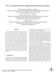
Our design goals for the GLOD API (see Figure 3) focus on
providing a lightweight model for the creation, management, and
rendering of geometry. To maximize its appeal to multiple
audiences, GLOD should be fast, extensible to different LOD
algorithms, and easy to integrate into existing applications.
Furthermore, it should allow incremental adoption rather than
locking developers into all pieces of the GLOD framework. To
accomplish these goals, GLOD API is tightly integrated with the
industry standard OpenGL API, so our design decisions are
guided as if GLOD were a component of OpenGL.
The data handled by GLOD is organized into three principal
units: patches, objects, and groups. A patch is the principal unit
http://www.cs.jhu.edu/~graphics/GLOD
Figure 1: The GLOD object and dataflow model.
12
of rendering. A patch is specified to GLOD using the OpenGL
vertex array interface. Drawing a patch is much like drawing a
vertex array, the chief difference being that what you get is an
LOD of the original arrays. The application may change rendering
state, such as bound textures, on a per-patch basis at the time of
rendering; GLOD does not interfere with rendering state.
An object is the principal unit of LOD generation. The application
designates one or more patches as an object before initiating
the LOD generation process. Thus multiple patches may be
simplified together into crack-free levels of detail. GLOD also
supports memory-efficient instancing of objects to provide
efficient LOD management for applications which render objects
in multiple locations.
A group is the principal unit of LOD management. An application
places one or more objects into a group. At each frame,
GLOD adapts the LOD of all patches of all objects in each group
according to the specified adaptation mode and current OpenGL
viewing matrices.
The GLOD pipeline is designed to allow flexible motion of
data into and out of it as desired by the application, as illustrated
in Figure 1. The original geometry is specified as patches using
the vertex array mechanism. The application can then set a
number of per-patch and per-object LOD generation parameters to
determine how the LOD hierarchy is constructed. For example,
parameters may be used to select a simplification operator, error
metric, hierarchy type (e.g. discrete, continuous, view-dependent),
importance values, etc. A special hierarchy type allows the
programmer to manually build discrete hierarchies from a set of
existing LODs. An entire hierarchy may be read back by the
application to save it to disk, allowing it to be re-used in a later
execution without regenerating it. Group parameters specify
management modes such as the error mode (object-space or
screen-space), adaptation mode (error threshold or triangle
budget), morphing parameters, etc. After adapting a group, the
individual adapted patches may be read back, again through the
vertex array mechanism. The application can store these vertex
arrays, pass them to OpenGL for rendering, etc. This complete set
of data paths allows applications to incrementally adopt GLOD.
3 DISCUSSION
We have currently limited the scope of GLOD to filtering geometric
detail without interfering with rendering state. This has several
benefits. The application may safely employ complex rendering
algorithms, including multi-pass algorithms, as well as custom
vertex and fragment programs. For example, applications can use
normal mapped LODs without difficulty in GLOD. Many user-

Figure 2: Bunny rendered in GLOD using a multipass
rendering algorithm, demonstrating GLOD’s policy of
non-interference with the underlying graphics system.
defined vertex program parameters can pass through GLOD
filtering. However, this is not applicable for all vertex programs.
Also, our non-interference policy makes some forms of LODs,
such as textured impostors, difficult to support because they
require us to change rendering state.
At the time of this writing, a pre-release version of the GLOD
system is available from our web site:
http://www.cs.jhu.edu/~graphics/GLOD
The current implementation supports both discrete and viewdependent
hierarchy formats, several simplification operators,
error threshold and triangle budget adaptation modes, etc. We
hope that this open source system will provide a viable and
convenient pathway for level of detail research to migrate from
the research lab to full deployment. With a wide array of simplification
algorithms, hierarchical data representations, and management
policies in their hands, all available through the setting of a
few parameters, application developers will have tremendous
power to select the implementations that meet their needs.
REFERENCES
Luebke, D., M. Reddy, J. Cohen, A. Varshney, B. Watson, and R.
Huebner. Level of Detail for 3D Graphics. Morgan Kaufman.
2003.
Rohlf, J. and J. Helman. IRIS Performer: A High Performance
Multiprocessing Toolkit for Real-Time 3D Graphics. Proceedings
of SIGGRAPH 94. July 24-29. pp. 381-395.
13
glodNewGroup(grpname);
glodDeleteGroup(grpname);
Create a group to contain and manage objects. Deleting
a group deletes all its objects.
glodNewObject(objname, grpname, format);
Create an object for a particular hierarchy format and
place in the named group.
glodInsertArrays(objname, patchname, mode,
first, count, level, error);
glodInsertElements(objname, patchname, mode,
count, type, indices,
level, error);
Put a patch into an object using vertex arrays. Level
and error can be used to load an LOD generated
elsewhere into a discrete hierarchy, but are typically
set to 0.
glodBuildObject(objname);
Complete an object and convert to hierarchy in the
selected output format.
glodInstanceObject(objname, instname, grpname);
Instantiate an existing object by sharing its geometry
hierarchy data, and place into a group.
glodDeleteObject(objname);
Delete an object (which removes it from its group).
glodBindAdaptXform(objname);
Capture an object’s viewing parameters for adapting
(not drawing – GLOD does not change the OpenGL
transformation state).
glodAdaptGroup(grpname);
Adapt LOD for all the objects in a group according to
the group’s ADAPT_MODE.
glodDrawPatch(objname, patchname);
Draw one patch of an object.
glodFillArrays(objname, patchname, first);
glodFillElements(objname, patchname, type,
elements);
Read back current adapted object into vertex arrays
glodGetObject(objname, data);
glodLoadObject(objname, data);
Read back an object’s hierarchy so it may be saved
and later reloaded to GLOD.
Figure 3: The GLOD API

Subjective Usefulness of CAVE and Fish Tank VR Display Systems for a
Scientific Visualization Application
1 Introduction
Ça˘gatay Demiralp David H. Laidlaw Cullen Jackson Daniel Keefe Song Zhang
cad, dhl, cj, dfk, sz@cs.brown.edu
Computer Science Department, Brown University, Providence - RI
The scientific visualization community increasingly uses VR display
systems, but useful interaction paradigms for these systems
are still an active research subject. It can be helpful to know the
relative merits of different VR systems for different applications
and tasks. In this paper, we report on the subjective usefulness
of two virtual reality (VR) display systems, a CAVE and a Fish
Tank VR display, for a scientific visualization application (see Figure
1). We conducted an anecdotal study to learn five domainexpert
users’ impressions about the relative usefulness of the two
VR systems for their purposes of using the application. Most of
the users preferred the Fish Tank display because of perceived display
resolution, crispness, brightness and more comfortable use.
Whereas, they found the larger scale of objects, expanded field of
view, and suitability for gestural expressions and natural interaction
in the CAVE more useful.
The term “Fish Tank VR” is used to describe desktop systems
that display stereo image of a 3D scene, which is viewed on a monitor
using perspective projection coupled to the head position of the
observer [Ware et al. 1993]. A CAVE is a room-size, immersive
VR display environment where the stereoscopic view of the virtual
world is generated according to the user’s head position and orientation
[Cruz-Neira et al. 1993].
Some related work compares Fish Tank VR displays with Head
Mounted Stereo Displays (HMD) and conventional desktop displays.
In [Ware et al. 1993; Arthur et al. 1993], the authors compare
Fish Tank VR with an HMD and conventional desktop systems.
[Pausch et al. 1997] showed that HMDs can improve performance,
compared to conventional desktop systems, in a generic search task
when the target is not present. However, a later study showed that
these findings do not apply to desktop VR; Fish Tank VR and desktop
VR have a significant advantage over HMD VR in performing
a generic search task [Robertson et al. 1997]. [Bowman et al. 2001]
compared HMD with Tabletop (workbench) and CAVE systems for
search and rotation tasks respectively They found that HMD users
performed significantly better than CAVE users for a natural rotation
task. For a difficult search task, they also showed that subjects
perform differently depending on which display they encountered
first.
Bowman and his colleagues’ work shares similar motivations to
ours. We go beyond their work with a direct comparison of CAVE
and Fish Tank VR platforms. Also, most of previous studies have
evaluated VR systems by looking at user performance for a few
generic tasks such as rotation and visual search on experiment specific,
simple applications. For most of the real visualization applications
it may be difficult to reduce the interactions into a set of
simple, generic tasks. Consequently, it is not clear how well the results
of these studies apply to real visualization applications. This
point is elucidated in a recent study that presented the importance of
application specific user studies using tasks that reflect end user’s
needs [Swan II et al. 2003]. In this study, the authors compare
user performance for an application specific task across desktop,
CAVE, workbench and display wall platforms. They found that
the users performed tasks fastest using the desktop and slowest us-
14
Figure 1: The visualization application running in the CAVE (left
image) and on the Fish Tank VR display (right image).
ing the workbench. They have a good discussion of the tradeoff
between application specific and generic user studies, stressing on
the value of application-context based user studies using high-level
tasks.
We chose to perform an anecdotal study for two specific reasons:
First, we believe application-oriented user studies using the
domain-expert user’s scientific hypothesis-testing process as a task
to be evaluated can be complementary to user studies that utilize
generic tasks and experiment specific applications. Second, we
wanted to gain insights for designing future quantitative studies to
compare user performance in CAVEs and on Fish Tank VRs.
2 Methods
Diffusion tensor magnetic resonance imaging (DT-MRI) is a new
imaging modality with the potential to measure fiber-tract trajectories
in fibrous soft tissues such as nerves and muscles. Our application
visualizes DT-MRI brain data as 3D streamtube and streamsurface
geometries in conjunction with 2D T2-weighted MRI sections.
It is based on the work by et al. [Zhang et al. 2001]. We have the application
running both in a CAVE and on a Fish Tank display. Five
domain-expert users were asked to use it both in the CAVE and on
the Fish Tank display. Our expert user pool was made of one neuroradiologist,
one neurosurgeon, one computer science graduate student
with an undergraduate degree in neuroscience, one biologist
and one doctor, who is also a medical school instructor, with an
undergraduate degree in computer science. Four of the users were
male and one was female. Two of the users started with the Fish
Tank version of the application and the rest with the CAVE version.
Each user had their own task (or scientific hypothesis to be
tested), which they described to us. They were asked to compare
the platforms with respect to their purposes. They did so by talking
to us while using the application. Most often we offered counterarguments,
which helped to expose the reasoning behind the users’
observations. The users were then asked to give an overall preference
for one of the two VR systems.
3 Results
Overall, one user preferred CAVE and four preferred Fish Tank VR
display. We summarize the users’ comments as to relative advan-

tages of CAVE and Fish Tank VR systems below.
Comments on advantages of CAVE:
¯ Has bigger models, one can see more
¯ Has larger field of view
¯ More suitable for gestural expression and natural interaction
¯ Possible to walk around
On Fish Tank VR display:
¯ Has sharper and crisper images
¯ Constitutes more information, relationships between the
structures are easier to see
¯ Feels more comfortable, non-claustrophobic and sitting is better
than standing
¯ Works better for collaboration, especially with two people
¯ Pointing to objects on the screen is easier
¯ More time efficient to use; doctors prefer to work-and-go
¯ Would work better for telemedicine-like collaboration
¯ More intuitive for surgery planning because doctors are used
to working with real or smaller brain sizes
Our first user was a neurosurgeon; he had used the application
before. He uses DT-MRI data to study obsessive-compulsive disorder
(OCD) patients and was particularly interested in studying
changes that occur after radiation surgery, which ablates an important
white matter region. He wanted to see the relation between the
neuro-fiber connectivity and linear diffusion (streamtubes) in the
brain. He strongly preferred using Fish Tank VR and did not find
any relative advantages of the CAVE.
Our second user was a biologist who was also trying to see correlations
between white matter structure and linear diffusion in the
brain. His interests were not confined to a specific anatomical region.
He was the only user who preferred the CAVE over Fish Tank
display.
Our third user was a doctor and a medical school instructor with
an undergraduate degree in computer science. She evaluated the
application from teaching and learning perspectives.
Our fourth user was a computer science graduate student with
an undergraduate degree in neuroscience. He looked at the application
to see correlations between white matter structures and linear
diffusion in the brain, similar to our second user. He said that he
preferred Fish Tank VR because 2D sections have higher resolution
and the models look crisper on the screen, which helped him see
the correlations easily.
Our last user was a neuroradiologist working on MS (multiple
sclerosis) disease. He wanted to see the 3D course of neurofibers
along corpus callosum. He was able to see what he was looking for
in both the platforms.
All users also found 2D sections to be very helpful in both platforms.
They said they were familiar with looking at 2D sections,
which help them to correlate and orient the 3D geometries representing
diffusion with the brain anatomy.
4 Discussion
The higher perceived display resolution, crispness, brightness, and
more comfortable use were considered useful on the Fish Tank VR.
On the other hand, users found the larger scale of objects, expanded
field of view, and potential use of gestural and natural interaction
useful in the CAVE. We believe that each of these factors is worth
investigating in order to quantify their effects on user performance.
Some of these factors have already been studied quantitatively: for
example, recently Kasik et al. showed the positive effect of a crisp
display on user performance [Kasik et al. 2002].
We still believe that application-oriented user studies using
the domain-expert user’s hypothesis-testing process as a task to
15
be evaluated can be complementary to user studies that evaluate
generic task performance on experiment specific, simple applications.
However, this approach is difficult to implement: First, one
needs many application-oriented studies to find meaningful patterns
and generalize them; second, finding enough expert users with similar
hypotheses can be very difficult.
In light of the experience we gained through this study, we hypothesize
that Fish Tank VR displays are preferable over CAVEs for
exocentric tasks, as they physically separate user’s reference frame
from the application’s. As an initial attempt to test this hypothesis
we will conduct a formal quantitative user study in which we
will compare the user performance between CAVE and Fish Tank
VR for an exocentric search task on a simple, experiment specific
application. However, we will also give a greater emphasis on the
task’s relevance in real visualization applications.
5 Summary
We presented results from an anecdotal user study with five
domain-expert users. They used a scientific visualization application
both in a CAVE and on a Fish Tank VR platform. While the
higher perceived display resolution, crispness, brightness and more
comfortable use were considered useful on the Fish Tank VR, users
found the larger scale of objects, expanded field of view, and potential
use of gestural and natural interaction useful in the CAVE.
Overall, one user preferred CAVE and four users preferred Fish
Tank VR.
References
ARTHUR, K.W.,BOOTH, K.S.,AND WARE, C. 1993. Evaluating 3d
task-performance for fish tank virtual worlds. ACM Trans. Inf. Syst. 11,
239–265.
BOWMAN, D. A., DATEY, A., FAROOQ, U., RYU, Y. S., AND VASNAIK,
O. 2001. Empirical comparisons of virtual environment displays. Tech.
rep., Virginia Tech Dept. of Computer Science, TR-01-19.
CRUZ-NEIRA, C., SANDIN, D. J., AND DEFANTI, T. A. 1993. Surroundscreen
projection-based virtual reality: the design and implementation
of the cave. In Proceedings of the 20th annual conference on Computer
graphics and interactive techniques, ACM Press, 135–142.
SWAN II, J. E., GABBARD, J. L., HIX, D., SCHULMAN, R. S., AND
KIM, K. P. 2003. A comparative study of user performance in a mapbased
virtual environment. In Proceedings of IEEE Virtual Reality 2003,
259–266.
KASIK, D.J.,TROY, J. J., AMOROSI, S.R.,MURRAY, M. O., AND
SWAMY, S. N. 2002. Evaluating graphics displays for complex 3d models.
IEEE Comput. Graph. Appl. 22, 56–64.
PAUSCH, R., PROFFITT, D., AND WILLIAMS, G. 1997. Quantifying immersion
in virtual reality. In Proceedings of the 24th annual conference
on Computer graphics and interactive techniques, ACM Press/Addison-
Wesley Publishing Co., 13–18.
ROBERTSON, G., CZERWINSKI, M., AND VAN DANTZICH, M. 1997.
Immersion in desktop virtual reality. In Proceedings of the 10th annual
ACM symposium on User interface software and technology, ACM Press,
11–19.
WARE, C., ARTHUR, K., AND BOOTH, K. S. 1993. Fish tank virtual
reality. In Proceedings of the conference on Human factors in computing
systems, Addison-Wesley Longman Publishing Co., Inc., 37–42.
ZHANG, S., DEM˙IRALP,Ç.,KEEFE, D., DASILVA,M., LAIDLAW, D. H.,
GREENBERG, B. D., BASSER,P.,PIERPAOLI, C., CHIOCCA, E., AND
DEISBOECK, T. 2001. An immersive virtual environment for dt-mri
volume visualization applications: a case study. In Proceedings of the
conference on Visualization 2001, IEEE Computer Society Press, 437–
440.

Abstract
Visual Exploration of Measured Data in Automotive Engineering
Andreas Disch, Michael Münchhofen, Dirk Zeckzer
ProCAEss GmbH
Landau, Germany
{A.Disch,M.Muenchhofen,D.Zeckzer}@procaess.com
The automotive industry demands visual support for the verification
of the quality of their products from the design phase to the
manufacturing phase. This implies the need of tools for measurement
planning, programming measuring devices, managing measurement
data, and the visual exploration of the measurement results.
To simplify and accelerate the quality control in the process
chain an integration of such tools in a platform independent framework
is crucial.
We present eMMA (enhanced Measure Management Application),
a client/server system that integrates measurement planning,
data management, and simple as well as sophisticated visual exploration
tools in a single framework.
1 Introduction
To ensure the quality of the fabrication process and the products
manufactured workpieces are measured using a coordinate measuring
machine. Measurement plans are based on the CAD models
usually stored in Product Data Management (PDM) or Product
Lifecycle Management (PLM) systems. Both systems are based on
a database and store also documents related with the CAD data.
The process chain of quality ensurance is made up of different,
partly complex steps, which are characterized by loosely coupled
software and nonuniform modi operandi. We have developed
eMMA to integrate those different procedures and the necessary
software into a single tool. Thus, we have the ability to integrate
new visualization types for the generation of evaluation reports.
We have designed a modular system that can be easily extended
to a wider spectrum of analysis algorithms, report styles, etc. It is
already in practical use in the automotive industry, but is, of course,
not restricted to car production. It can be used in any mechanical
engineering or production business.
2 System Overview
Main areas of our system eMMA include the Measurement Plans
and Report Templates, the Online Evaluation, and the creation and
printing of Measuring Reports. We describe these areas in the subsequent
sections.
2.1 Measurement Plans and Report Templates
The whole system is centred around the MDM (Measure Data Management)
database which stores assembly hierarchies along with
measurement plans, measuring data, report definitions, evaluation
definitions, references to the PDM system, etc.
Figure 1 shows the MDM tree on the left side and an information
panel on the right side which displays information about the
currently selected node. After selecting the menu item for editing
a report template and choosing an existing or starting the definition
of a new report template the main window looks like in figure 2.
16
Ralf Klein
IVS, DFKI GmbH
Kaiserslautern, Germany
Ralf.Klein@dfki.de
Figure 1: The eMMA main window displaying a tree of product
types, component parts, and measurement plans stored in the MDM
database
The structure of the current template is displayed in the left panel
where the user can add, edit, or remove report views, or move features
from one view to another. The right panel shows the main
image of the currently selected view. A viewing editor allows the
user to pan, rotate, and zoom the view on the geometry and to take
snapshots which are stored with the current view.
Figure 2: The definition of a report template organized in several
report views (pages) with report features attached to them
In the online evaluation module we have implemented several
different views on the measured data of quality features on a selected
assembly to meet different needs of an evaluator.
From the main window (see figure 1) the user gets to the evalua-

tion module by first selecting a measurement plan in the MDM data
tree and then choosing the Evaluation action. This switches to the
evaluation module where the user can either run an online evaluation
with the default report template or he can first open a settings
dialog to make more specific selections.
When the online evaluation is complete we list all evaluated
quality features with their nominal data and the computed error values
for each measuring in a table. Errors that are out of tolerance
bounds we colour red. We also display the main image of the current
active report view.
Figure 3: Online evaluation of a component showing the error values
for each quality feature and each measuring as well as a graphical
representation of the workpiece
To aid the user in finding the measured quality features in the
picture on the right side we compute and render labels pointing to
the features’ locations (like in figure 2).
One of the other possible types of online evaluation that can be
started by right-clicking on the table is the Cpk online evaluation
that is shown in figure 4. By moving the vertical edges of the blue
area horizontally the user can deselect an interval of measurings
from being used for the computations of the values listed on the
left. The user may also right-click the points to select/deselect a
single measuring.
Figure 4: Cpk online evaluation of a round hole: hashed out measuring
results are discarded for Cpk computation
Very similar to the Cpk online evaluation is the analysis tool that
also opens a frame showing a trend chart for each evaluated dimension
and a table with some statistical data (see the lower trend
17
chart window in figure 5). We offer this tool for convenience reasons
for users who don’t need the actual Cpk computation function.
When the mouse hovers over points representing measuring results
we show tool tips that reveal an identifier of the measuring process,
the measured value, and the error value which is colour-coded.
Figure 5: A collection of several online evaluation functions
2.2 Measurement Reports
Beside the different types of online evaluation within eMMA we
also allow the user to generate PDF files with customizable layout
schemes. In a first step we implemented an export of evaluation
and report data in an XML file which then was transformed by XSL
stylesheets into a PDF file. These XSL stylesheets actually define
the report style and can be easily integrated to allow any kind of
report.
Currently, we are working on a way to directly create PDF files
from our internal data structures. This will improve the performance
on generating standard reports while the XML interface still
enables an easy way for integrating user-specific plug-ins.
3 Conclusions
We have presented an integrated system providing visual support
to meet the needs of the manufacturing industry for quality control
through the whole product lifecycle. We have combined tools for
managing measurement plans, the results from measurings, and for
the visual exploration of the measuring results.
Compared to the conventional method of using a loose collection
of tools our integrated solution eMMA means a decisive improvement
in today’s quality control work flow. We provide the means
for a robust process chain without the risk of data inconsistencies.
Beside the advantage of only one interface to be learnt we also
offer the incorporation of any report style As further advantages,
the users don’t need to learn different user interfaces and they don’t
need to change between different applications. This leads to an
accelerated quality control process and efficiently aids in improving
the product quality.

Free Form Deformation for Biomedical Applications
Shane Blackett, David Bullivant, Peter Hunter
Bioengineering Institute, The University of Auckland, New Zealand
http://www.bioeng.auckland.ac.nz
Free form deformation is a useful technique for customisation and specification of anatomical finite
element models.
Introduction
The IUPS Physiome Project is a worldwide effort to provide a computational framework for
understanding human physiology. Working towards this goal finite element models have been
created for many parts of human anatomy and the use of free form deformation is integral to the
model creation, customisation and visualisation.
Free form deformation has been described in computer graphics applications for a number of years.
(Sederberg and Parry 1986) and direct-free form deformation introduced the concept of using a
least squares minimisation (Hsu et al. 1992).
The whole organ models that have been developed generally incorporate cubic Hermite finite
elements providing a C1 continuous description of geometry with a relatively small number of
elements. They are used to calculate mechanics, electrical excitation and embedded vessel fluid
flow. Software developed at the Bioengineering Institute (CMISS http://www.cmiss.org) is used
for computation and visualisation.
Most of the applications of free form deformation in the Bioengineering Institute employ a similar
process. Identifiable common points are selected on an existing model and on the target dataset,
either manually or with some image processing. The objects are aligned as solid bodies, then the
existing model is embedded in a host mesh, which is usually a small number of tricubic Hermite
elements. A least squares fit is performed to find the nodal positions and derivatives in the host
mesh which minimise the distances between the model and target points. The target points can be
weighted differently and Sobelov smoothing can be applied to each of the degrees of freedom of the
host mesh.
Host Mesh Model Mesh
Model Point Target Point
a b
c
d
Figure 1 (a) The initial model geometry and a host mesh which contains it. (b) Model point and
target point pairs are specified. (c) A close up illustration from b. (d) The fitted geometry showing
the deformed host mesh, the deformed model and the residual vectors where the target points were
not matched exactly.
Heart Fibres
In cardiac tissue there is a definite fibre direction, and these fibres are coupled into sheets giving the
myocardium a very anisotropic material behaviour. The fibre alignment varies throughout the heart
18

wall. These important fibre and sheet directions were carefully measured by hand for a single heart
(Nielsen). To enable mechanics solutions to be generated on other heart models it is important to
have a representation of this fibre field but the effort required to acquire another set of fibre
alignments has been prohibitive. By using free form deformation the existing fibre field can be
transferred from the existing hand measured models to other ventricular models.
Model Specification
A detailed model of each bone, muscle and ligament around the knee joint has been developed from
the Visible Human data set (Fernandez). To facilitate patient specific analysis of the stresses in the
knee, a model that is customised to that patients geometry is required. To create this a single scan is
obtained and then free form deformation used to align the existing detailed model with the scan.
Similarly the Bioengineering Institute's lung models are customised to specific lung geometry
segmented from scans by free form deformation.
a b c d
Figure 2 (a) Generic model of the femur. (b) Cloud of scanned data from a particular patient. (c)
Fitted femur in deformed host mesh. (d) Close up of the fitted femur (red).
Facial Animation Performance
Facial animation requires models which represent the dynamics of the skin surface. By acquiring
detailed motion capture of a particular performance these dynamics can be reproduced digitally. By
using free form deformation to provide a mapping from two different neutral faces, the dynamic
performance can be transferred through the same mapping, allowing dynamics captured from one
animation to be transferred to any number of other models.
a b
Figure 3 (a) A generic standard model showing a smile. (b) Free form deformation was used to
transfer dynamics, including the smile to a significantly different shaped face.
Fernandez, J.W., Mithraratne, S., Thrupp, M. H., Tawhai, M. H. & Hunter P. J. 'Anatomically based geometric
modelling of the musculo-skeletal system and other organs' To appear in Biomechanics and Modelling in
Mechanobiology.
Nielsen, P. M. F., LeGrice, I. J., Smaill, B. H. & Hunter, P, J. (1991) 'Mathematical model of geometry and fibrous
structure of the heart', Am. J. Physiol. Heart Circ. Physiol. 260(29), H1365-H1378
Sederberg, T.W. & Parry, S. R. (1986) 'Free-Form Deformation of Solid Geometric Models', ACM Computer Graphics
(SigGraph 86 Conference Proceedings) 20(4), 151-160
19

Ming C. Hao
HP Research Labs
Palo Alto, CA
1 Introduction
Daniel A. Keim
University of Constance
Germany
The automation of activities in almost all areas, including business,
engineering, science and government produces an ever increasing
stream of data. Even simple transactions of every day life, like
credit card payments or telephone calls are logged by computers.
Most of these transactions have a spatial location attribute, like
source and destination of a telephone call or location of a credit card
payment [Keim and Herrmann 1998]. This data is collected because
it is a potential source of valuable information. For business
analysts, for example, it is important to know the sales amount for a
certain product or the customer behaviour for geographical regions
like the states of a country. In this poster we combine the ability of
Pixel Bar Charts [Keim et al. 2002] and interactive maps for visualising
multidimensional data belonging to certain geographical regions.
The user can choose a geographical region on an interactive
map and analyse the collected data assiciated with this region using
the Pixel Bar Chart technique. The advantage of Geo Pixel Bar
Chart is that the underlying data can be partitioned in geographical
regions, and at the same time, all data items of each of the regions
can be visualised without aggregation.
2 Geo Pixel Bar Chart System
The Geo Pixel Bar Charts system consists of an interactive map
and Pixel Bar Charts. The user can choose geographical regions
of a map by clicking the corresponding polygon on the interactive
map. Once the user has select a region on the map, a Pixel Bar
Chart for the underlying data of this region is computed. The user
then selects different dimensions of the categorical data for the partitioning
into bars. Then the user navigates over pixels within the
bars to analyze detailed information of the data record. Figure 1 illustrates
the interaction capabilities between the map and Pixel Bar
Charts.
Figure 1: Screenshot of the Geo Pixel Bar Chart System
2.1 Interactive map
An interactive map is used in the Geo Pixel Bar Chart System. The
user interacts with the map by either clicking on single geographical
Geo Pixel Bar Charts
Umeshwar Dayal
HP Research Labs
Palo Alto, CA
20
Joern Schneidewind
HP Research Labs
Palo Alto, CA
Peter Wright
HP Finance
Atlanta, GE
regions on the map to start Pixel Bar Charts for the underlying data
of this region, or starts Pixel Bar Charts for the global map. A feature
of the map is the visualization of additional statistical or business
attributes, like population density, income, or sales amount,
expressed by the color of the map regions. The map is connected to
Pixel Bar Charts. If the user selects an item in the Pixel Bar Charts,
the region in the map corresponding to the spatial attribute of the
data item is highlighted.
2.2 Pixel Bar Charts
Pixel bar charts are derived from regular bar charts. The basic idea
of a pixel bar chart is to present the data values directly instead of
aggregating them into a few data values. The approach is to represent
each data item (e.g. an invoice) by a single pixel in the bar
chart. The detailed information of one attribute of each data item is
encoded into the pixel color and can be accessed and displayed as
needed. To arrange the pixels within the bars one or two attributes
are used to separate the data into bars and then use two additional
attributes to impose an ordering within the bars. Pixel Bar Charts
realizes a visualization in which one pixel corresponds to one data
item and can therefore be used to present large amounts of detailed
information.
Figure 2: Basic Idea of Space Filling Pixel Bar Charts
In the Geo Pixel Bar Chart system, Space-Filling Pixel Bar
Charts are used in order to increase the number of displayable data
values on the available screen space. The basic idea is to is to use
equal-height instead of equal-width bar charts, shown in Figure 2.
3 Applications
The Geo Pixel Bar Chart technique has been applied to sales
analysis and Internet usage analysis at Hewlett Packard Laboratories.
The applications show the wide applicability and usefulness
of Geo Pixel Bar Charts.
3.1 Sales Analysis
The rapid growth of business on the Internet has led to the
availability of large volumes of data. Business research efforts have
been focused on how to turn raw data into actionable knowledge.
In order to find and retain customers, business analysts need to
improve their sales quality based on prior information. For sales
analysis, sales specialists would like to discover new patterns and

elationships in the invoice data. Common questions are ‘What is
the sales growth rate in recent months?’, ‘Which product has the
most sales?’, and ‘Where do the sales come from?’. With Geo
Pixel Bar Charts it is easy to explore all sales for a geographical
region and obtain additional information from the Pixel Bar Chart
visualization.
Figure 3: Geo Pixel Bar Charts for California: partition attribute is
day, ordering attribute is dollar amount
Figure 3 shows an interactive geographical map. The highlighted
yellow region (California) corresponds to the region the user has
clicked. The pixel bar chart represents the underlying data for this
region. In this example, a data file with sales transaction for a certain
company is used. The pixel bar chart shows the sales growth
rate for the state California over 37 days. Each pixel in the pixel
bar charts corresponds to a customer invoice. Within the bars, the
pixels are ordered by dollar amount. The color of the map regions
represents the population density. Blue regions have a high density
and red regions have a low density. Thus an analyst might be
more interested in high populated areas instead of areas with low
population density.
3.2 Internet Usage Analysis
Geo Pixel Bar Charts have also been used to analyze Internet
duration time at Hewlett Packard Laboratories. A system analyst
can use the visualization to rapidly discover event patterns to
manage the Internet configuration. With an interactive map, the
analyst might be able to find server locations which might be the
source of Internet traffic problems or can locate geographical regions
with high internet traffic duration time. This application also
demonstrates that Geo Pixel Bar Charts is interactive in two ways.
The user can click on a region in the interactive map to start a Pixel
Bar Chart for this region. The user can also start with a Pixel Bar
Chart to explore the geographical location of each of the data items
in the chart by clicking on the data item. If the data item has a
21
spatial location attribute, this location is highlighted on the interactive
map. To map the logged IP addresses to geographical locations
a geo-locator database is employed.
Figure 4: Location of IP addresses: If the user clicks on a data item,
the geographical location of this item is highlighted as a circle in the
map. The color of this circle corresponds to the color of the item.
Most web traffic occurs between hours 9 and 17.
Figure 4 presents an Internet access log file visualized by Geo
Pixel Bar Charts. The data items contained in the Pixel Bar Charts
correspond to web transactions. The partitioning attribute is hour of
the day and the y-ordering attribute is duration time. If the web request
exceeds a threshold duration time (100ms) the corresponding
data item is colored red. If the analyst clicks on a data item in the
Pixel Bar Chart, the corresponding geographical location is highlighted
on the map. This makes it easy to find regions with high
duration time or locations with high volume of web requests.
4 Conclusion
This poster presents a new interactive visualization technique called
Geo Pixel Bar Charts, which combines the advantages of interactive
maps and Pixel Bar Charts. Further research goals will focus on
the improvement of the new technique and the use of distortion
techniques like cartograms instead of normal maps.
References
KEIM, D. A., AND HERRMANN, A. 1998. The gridfit algorithm: An
efficient and effective approach for visualizing large amounts of spatial
data. In Proc. Visualization ’98, Research Triangle Park, NC, 181–188,
531.
KEIM, D. A., HAO, M. C., DAYAL, U., AND HSU, M. 2002. Pixel bar
charts: A visualization technique for very large multi-attribute data sets.
Visualization, San Diego 2001, extended version in: IEEE Transactions
on Visualization and Computer Graphics 7, 2002.

1. MOTIVATION
3D models are becoming ever more detailed as the number of
triangles representing these models increases. As a surface gets a
more detailed representation, more triangles of smaller sizes are
used. When these small triangles are rendered on screen, each
may cover only a few pixels. As such, point was proposed as an
alternative primitive [2].
We observe that there is a gap between the two known primitives
of point and triangle in representing and rendering 3D models or
surfaces; that is, the line, in particular anti-alias line has yet to be
studied. Our work is also motivated by the observation that while
point is suitable for surfaces with high complexity and irregularity
and triangle for regular surfaces, line is suitable for surfaces with
regularity along one dimension (such as a cylindrical surface).
Figure 2 shows an arm bone where lines or hybrid of lines and
points can represent it concisely as most parts of its surface have
regularity along one dimension. Without the line primitive, a
surface with regularity along one dimension may need to be
represented unfavourably by thin or fat triangles, many smaller
triangles, or many points. Another view of this motivation is the
compression that lines can provide. Given an arbitrary set of
points, it may be possible to come up with heuristics to construct a
set of lines which represents a larger set of points while
maintaining a certain error measure.
In another view, having the line primitive, one can construct a
model and its different level of details (lods) with a continuous
spectrum of primitives. From the intra-primitive perspective, for a
polyline, the error measure of its lod as another polyline can be
formulated in some straightforward way. From the inter-primitive
perspective, a primitive can be replaced with another primitive
depending on the position of the viewpoint: if a triangle is far
away, it projects as a small triangle which can be represented by a
line and subsequently as a point. We note that the line primitive
can be adaptive in that the same line is used to represent near or
far surfaces, but if a set of points is used in place of a line, to
maintain surface continuity, a sufficient number of points we need
to use when the surface is near is more than that is needed when
the surface is far away.
In this work, we formulate the line primitive as another
representation and rendering alternative. It extends the antialiasing
theory in texture mapping [1] to render anti-aliased 3D
line models. Our work on rendering line is also using the elliptical
weighted average (EWA) resampling filter [3, 4, 5].
2. DESCRIPTION OF THE IDEA
Our work started with finding a solution for the resampling filter
of lines. We attempted to find a closed form solution since there
exists closed form approximation for the integration of Gaussian
points along a line, as a Gaussian line, using the error
3 Science Drive 2, Singapore 117543, Republic of Singapore.
Emails: keenhon@hotmail.com, ouyangxi@comp.nus.edu.sg,
tants@comp.nus.edu.sg
Line Rendering Primitive
Keen-Hon Wong Xin Ouyang Tiow-Seng Tan
School of Computing, National University of Singapore
22
1
Figure 1: Opaque, transparent and textured line models
rendered by our approximation method.
function erf (x)
. We, however, arrived at an expression which in
general, cannot be integrated in closed form. Instead, we have
designed a good approximation to render anti-aliased opaque,
transparent and textured 3D line models; see Figures 1 and 3.
A simple view of our approximation idea is to linearly interpolate
between two EWA resampling filters computed at the line
segment endpoints. More specifically, our approximation is based
on the analysis of the texture mapping theory with consideration
of the properties of perspective mapping and Gaussian
convolution. Following is a brief description of the process to
render a line; all rendered lines are to be blended as in [5].
Ellipse equations for the two EWA resampling filters at both
endpoints of a line are computed. These equations are then used to
compute the tangent lines ( 1, 2 and 3,4 ) connecting the two
ellipses and vertices 5 to 18 as shown in Figure 4. These 18
vertices are then used in the mapping of the Gaussian influences
while minimizing possible distortion. The Gaussian influences are
pre-computed from a Gaussian line of length l > 2, r where r is

Figure 2: Arm bone represented by different primitives.
Figure 4: Texturing lines’ contents with influence textures.
the cutoff radius of a unit Gaussian kernel. The pre-computed
influence is then sliced into a side and a middle texture which are
used for the endpoints portion and middle portion respectively.
Next, the line is coloured or mapped with texture images.
3. RESULTS
We implemented a software pipeline in C/C++ and conducted
experiments for both lines and points primitives. The lines and
points models we acquired are converted from triangle models. In
the experiments we compare the quality and performance of
rendering different models using points, lines, and a hybrid of
points and lines. We also scrutinize the results of linearly
interpolating texture mapping. A video of the rendering results is
at http://www.comp.nus.edu.sg/~tants/line.html.
From our experiments, the numerical results (image difference
between a rendered line model and a point model) show that the
rendered line and point models have the same quality. Indeed,
there is no significant difference detected visually between each
pair of images from a line and its corresponding point model.
Based on our experiments, the estimated cost of rendering a line is
equal to rendering 4.3 points.
We also created hybrid models (combination of lines and points).
In conjunction with the result in the last paragraph, we find that
the optimum hybrid model will need to convert lines which are of
length less than the maximum distance covered by 4 points. We
intend to perform more experiments on different platforms to
better understand the tradeoff between lines and points.
As for texture mapping line models, shorter lines cause less
amount of interpolation error compared to longer lines.
Additionally, due to the perspective mapping and linearity of
lines’ texture coordinate interpolation, it is indeed the case that the
23
Figure 3: Opaque (top) and transparent (bottom) anti-aliased
checkerboard line models. Each line is painted with only one color
and lines of different colors are separately laid in checker boxes.
problem of texture mapping error is worsened for lines oriented in
the viewing direction. Our preliminary investigation shows that
the cost of rendering a textured line to be equivalent to rendering
about 5 points. An example of a textured model is the face model
as shown in Figure 1.
4. CONCLUDING REMARKS
We are currently investigating ways to convert raw data (for
example, 3D scanned points) directly to lines and also tools to
support hybrid modeling using any combination of points, lines
and triangles. To increase the rendering performance of the
primitive, we are also looking into implementing the
approximation using existing graphic hardware acceleration.
Other possible research includes new data structures and
algorithms to support inter-primitive and intra-primitive level-ofdetail
models.
References
[1] P. Heckbert. Fundamentals of Texture Mapping and Image
Warping. Master’s Thesis, University of California,
Berkeley, June 1989.
[2] M. Levoy and T. Whitted. The Use of Points as a Display
Primitive. Technical Report TR 85-022, University of North
Carolina at Chapel Hill, 1985.
[3] H. Pfister, M. Zwicker, J. van Baar, M. Gross. Surfels:
Surface Elements as Rendering Primitives. In Proc. of
SIGGRAPH 2000, pp. 335–342, July 2000.
[4] L. Ren, H. Pfister, M. Zwicker. Object Space EWA Surface
Splatting: A Hardware Accelerated Approach to High
Quality Point Rendering. In Proc. of Eurographics 2002, pp.
461–470, September 2002.
[5] M. Zwicker, H. Pfister, J. van Baar, M. H. Gross. Surface
Splatting. In Proc. of SIGGRAPH 2001, pp. 371–378, July
2001.

Visual Exploration of Association Rules
Li Yang ∗
Department of Computer Science, Western Michigan University
Frequent itemsets and association rules[Agrawal and
Srikant 1994] are difficult to visualize. This is because that
they are defined on elements of the power set of a set of
items that reflect the many-to-many relationships among the
items. With the absence of effective technique to visualize
many-to-many relationships, association rules pose fundamental
challenges to information visualization.
We begin by defining a few terms: An itemset is a set of
items. A transaction supports an itemset if the transaction
contains all items in the itemset. Support of an itemset
A, support(A), is defined as the percentage of transactions
that support A. The support of a rule A → B is defined
as support(A ∪ B). The confidence of the rule A → B is
defined as support(A ∪ B)/support(A). An item group is a
transitive closure of items in a set of frequent itemsets or
association rules. Mining generalized association rules with
item taxonomy was proposed in [Srikant and Agrawal 1995].
An example item taxonomy tree that organizes the items
{a, b, c, d} is shown in Figure 1. A transaction T supports
an item a if a ∈ T or a is an ancestor of some item in T under
the item taxonomy. A transaction T supports an itemset A
if T supports every item in A. An ancestor itemset A of A
is obtained by replacing one or more items in A with their
ancestors. A is then called descendent itemset of A.
Frequent itemsets are downward closed according to the
subset relationship and the ancestor relationship. Let I
be the set of all items and IT be an item taxonomy
on I. Let P(I) denote the power set of I. Define the
generalized power set GP(I, IT) as GP(I, IT) = P(I) ∪
{ancestor itemsets of A|∀A ∈ P(I)}, that is, GP(I, IT) contains
all possible itemsets and their ancestor itemsets. Define
partial order as: (1) A B if A ⊆ B; (2) A A.
Then < GP(I, IT), > is a lattice. It is easy to verify
that support(A) ≥ support(B) if A B. Therefore,
there is a border in < GP(I, IT), > which separates
the frequent itemsets from the infrequent ones. Figure 2
shows an example support border in the generalized lattice
< GP(I, IT), > on the items I = {a, b, c, d} under the item
taxonomy in Figure 1. We use straight lines to denote subset
relationships and arcs to denote ancestor relationships.
An item taxonomy tree can be partly displayed in a visualization,
beginning from its root and stopping at any internal
nodes. An itemset is called displayable if all items
in the itemset are shown in the displayed taxonomy tree.
The displayable property is downward closed in the generalized
itemset lattice < GP, >. Therefore, we have now two
borders in < GP, >: one border separates the frequent
itemsets from infrequent ones; the other border separates
the displayable itemsets from indisplayable ones. For example,
assume that the item taxonomy tree in Figure 1 is
partly displayed so that only the items c, d, e, f are visible
and items a and b are invisible, this specifies a border of
displayable itemsets which is also shown in Figure 2.
We can design a visualization method so that only nonredundant
displayable frequent itemsets are displayed. Here
non-redundant means that the frequent itemset is not im-
∗ e-mail: li.yang@wmich.edu
24
f
e f
a b c d
Figure 1: A simple item taxonomy tree.
{ }
a b c d
af bf ab ac ad bc bd cd ec ed ef
abf
abc abd acd bcd
abcd
e
ecd
Displayable
itemset
border
Figure 2: The lattice < GP(I, IT), >.
Support
border
plied by any other displayed frequent itemsets. In the lattice
< GP, >, the non-redundant displayable frequent itemsets
must reside on the border of the intersection of frequent
itemsets and displayable itemsets. Taking Figure 2 for example,
ec and ed are two such itemsets on this border and
should be visualized. The other displayable frequent itemsets
are implied by these two itemsets.
Association rules generated from a frequent itemset have
also closure property. Let A be a frequent itemset and
B ⊆ A, then B → (A − B) is an association rule if the
support support(B) does not exceed support(A)/minconf
where minconf is the user-defined minimum confidence. This
means that the association rules generated from a frequent
itemset are upward closed according to their LHSs in the
sub-lattice formed by the frequent itemset using subset relationship
as the partial order. This means that, if a → bc is
a valid rule, then ab → c and ac → b are valid rules that can
pass the same support and the same confidence tests. Furthermore,
a → b, a → c, a → ˆ bc, a → bĉ are also valid rules.
We have developed algorithms for generating displayable frequent
itemsets and for generating association rules that are
not implied by any other rules.
Parallel coordinates have often been used[Inselberg 1990]
to visualize relational records. We propose to use it to visualize
data with variable lengths such as frequent itemsets and
association rules. Figure 3(a) illustrates the visualization of
three frequent itemsets adbe, cdb and fg as polygonal lines.
Items are arranged by item groups so that items belonging
to the same group are displayed together. In this way, the

g
f
e
b
d
c
a
g
f
e
b
d
c
a
g
f
e
b
d
c
a
g
f
e
b
d
c
a
(a)
(b)
g
f
e
b
d
c
a
g
f
e
b
d
c
a
g
f
e
b
d
c
a
g
f
e
b
d
c
a
Figure 3: Visualizing (a) frequent itemsets and (b) association
rule.
g1
f1
e1
b1
d1
c1
a1
g2
f2
e2
b2
d2
c2
a2
p0
p1
p2
g3
f3
e3
b3
d3
c3
a3
p3
g4
f4
e4
b4
d4
c4
a4
Figure 4: Visualizing association rules using Bezier curves.
polygonal lines are organized into “horizontal bands” and
never intersect with each other. Figure 3(b) illustrates the
visualization of an association rule ab → cd. An association
rule is visualized as one polygonal line for its LHS, followed
by an arrow connecting another polygonal line for its RHS.
This method provides a way to support the closure properties:
Subsets of displayed frequent itemsets are implied
frequent. ab → cd implies that abc → d, abd → c, ab → c
and ab → d are all valid rules. If two or more itemsets or
rules have parts in common, for example, adbe and cdb in
Figure 3(a), we can use cubic Bezier curves instead of polygonal
lines to distinguish one from the other. Two example
rules, ab → ce and db → ce, are visualized in Figure 4 by
using Bezier curves.
We demonstrate our method by using a supermarket
transaction data in IBM DB2 Intelligent Miner as the test
data. The data contain 80 items which are leaf nodes of a
4-level taxonomy tree. 496 frequent itemsets are discovered
when the minimum support is set to 5%. The visualization
begins by displaying [Root] nodes. As the user clicks on a
node and expands the item taxonomy tree, frequent itemsets
will be displayed. Figure 5 visualizes frequent itemsets on a
partly shown taxonomy tree. The color of the name of each
item or item category represents its support. Displayable
frequent itemsets are visualized as smooth connections of
Bezier curves. The color of a curve represent the support
value of the corresponding itemset. The user can select an
itemset by clicking anywhere on its curve segments. The
selected itemset and its implied itemsets will be printed out
with their support values.
Figure 6 shows a visualization of the discovered association
rules when the minimum support is set to 5% and
25
Figure 5: Frequent itemsets drawn on the selected items.
Figure 6: Association rules drawn on the selected items.
the minimum confidence is set to 50%. Association rules
are aligned according to where the RHSs separate from the
LHSs. In this example, the left two coordinates represent
the LHSs of the rules and the right two coordinates represent
the RHSs of the rules. Support of a rule is represented
by line width. Confidence of a rule is represented by color.
All these visualizations also support panning and zooming.
The fundamental problem in the visualization of frequent
itemsets and association rules is that there is a long border of
frequent itemsets in the generalized itemset lattice and there
is no visual technique directly applicable to displaying manyto-many
relationships. We have overcome this problem by
using an expandable item taxonomy tree to organize items.
Basically this introduces another border which separates the
displayable itemsets from the non-displayable ones. Only
those frequent itemsets that are on this border are displayed.
By changing this border through expanding or shrinking the
display of the item taxonomy tree, we selectively visualize
frequent itemsets and association rules that we are interested
in.
References
Agrawal, R., and Srikant, R. 1994. Fast algorithms for mining
association rules. In Proc. 20th Int. Conf. Very Large Data
Bases (VLDB’94), 207–216.
Inselberg, A. 1990. Parallel coordinates: A tool for visualizing
multi-dimensional geometry. In Proc. 1st IEEE Conf. Visualization,
361–375.
Srikant, R., and Agrawal, R. 1995. Mining generalized association
rules. In Proc. 21st Int. Conf. Very Large Data Bases
(VLDB’95), 407–419.

×ØÖ Ø
ÅÙÐØ ÄÚÐ ÓÒØÖÓÐ Ó ÓÒØÚ Ö ØÖ× Ò ÎÖØÙÐ ÒÚÖÓÒÑÒØ×
Peter Dannenmann Henning Barthel Hans Hagen
We present our approach for a general component-based animation
framework for autonomous cognitive characters. In this ongoing
project we develop a working platform for autonomous characters
in dynamic virtual environments, where users can define high
level goals, and virtual characters will determine appropriate actions
based on specific domain knowledge and AI techniques. The
user will also be allowed to overrule the character’s decision and
force it to execute different actions. Motion sequences implied by
the character’s actions will be created by adapting reference motions
provided by a motion database.
CR Categories: I.2.0 [Artificial Intelligence]: General—
Cognitive Characters; I.3.7 [Computer Graphics]: Threedimensional
Graphics and Realism—Animation;
Keywords: character animation, cognitive characters, animation
framework
ÁÒØÖÓÙ ØÓÒ
In the last years, animation and simulation of human characters in
virtual environments has become ever more important in numerous
areas of applications. Besides movie, gaming and advertising companies,
also manufacturing industry has discovered the benefit of
integrating virtual humans into their development process.
Although today’s commercially available animation packages
provide advanced tools like key-frame editors, inverse kinematics,
etc. the creation of high quality animations is still expensive, and
especially dependent on skilled artists, animators or programmers.
However, the design of computer animations also is an enormous
creative process and quite a lot of modification will occur, until a
”generally” accepted result has been achieved. That means, until
a final version of an animation has been generated, a lot of refinements
considering the building of characters and environments, as
well as their number, type and distribution have to be handled. All
this requires significant manual animator intervention.
Therefore, providing a higher degree of automation in this process
is vital. Incorporating Artificial Intelligence technology within
animation generation tools and procedures can efficiently support
this task. Especially, introducing flexibility and adaptability to the
virtual character’s behavior with respect to changing roles or a dynamically
changing environment as well as techniques for reusing
already existing motion sequences are of major interest.
£ email: [dannenbarthelhagen]@dfki.uni-kl.de
German Research Center for Artificial Intelligence £
26
ÒÑØÒ ÓÒØÚ ÎÖØÙÐ Ö ØÖ×
Over the decades, computer animation has evolved from a purely
geometrical based manipulation technique to a more powerful simulation
of models by including physical principles (see e.g. [Watt
and Watt 1992], [Kokkevis et al. 1996], [Sun and Metaxas 2000]).
The fundamental motivation behind that entire endeavor is the
automation of a variety of difficult animation tasks which especially
include the creation of realistically looking and moving virtual
characters. Traditional approaches to meeting those requirements
were to employ highly skilled human animators who were
using the labor-intensive keyframing technique.
After including physical principles into the animation generation
process, the next substantial progress has been the introduction of
behavioral animation techniques ([Brogan et al. 1998], [Cavazza
et al. 1998], [Chen et al. 2001]).
Adding a cognitive layer on top of the behavioral level (see e.g.
[Funge 1999]) allowed the caracters to act quite autonomously and
react quite flexibly to changes in their environment. However, the
direct interaction of the characters with dynamic environments as
well as permitting control of the characters on all three levels of
control in parallel (i.e. on direct control level, on behavioral level
and on cognitive level) are still challenging subjects of research.
Ì ÇÆÌÌ ÖÑÛÓÖ
In the course of the project CONTACT [Barthel et al. 2003] topics
related to the generation and automatic adaptation of low-level
(key-frame) motions of virtual characters as well as topics related
to the multi-level directability of autonomous characters are investigated.
The resulting system will enable the user to define animations
on a high-level basis mainly by specifying a goal for a virtual
character. Based on the given domain knowledge the character automatically
will work out an appropriate action plan. Additionally,
the user will be allowed to overrule the character’s decision and
for example force the character to fall back on some predefined behavior.
When an action implies the movement of a character, the
corresponding motion sequence will be created by automatically
adapting reference motions provided by a motion database.
The generation of animations within the CONTACT framework
is an iterative process. Starting from a given description of the cognitive
characters’ environment and situation, they initially plan their
actions. After the planning is completed the plans are going to be
executed by animating the characters. Due to the dynamic nature
of the environment, changes (probably caused by the virtual characters,
moving environment objects or by user interaction) may occur
that make the current plans obsolete. This causes the characters
involved to perform a re-planning taking into consideration the
changed environment.
Based on the actual plan the animation is generated by combining
motion sequences of atomic actions. These atomic actions are
stored within a motion database and are adapted to the executing
character’s anthropometry and then combined to the animation sequence
(see figure 1).
The generation of the cognitive characters’ action plans is based
on Funge’s work ([Funge 1998]) on the Cognitive Modeling Language
(CML) that in turn has it’s foundation in the Situation Calcu-

Cognitive Cognitive Character Character
(Java) (Java)
Animation-Plan
Animation-Plan
User User Interaction Interaction
Event/Interrupt/Control
Data/Relation
Animation Animation Control Control
(Java) (Java)
Primitive/Atomic
Primitive/Atomic
Actions
Actions
Legend
Data/Document
Data/Document
Environment Description
Environment Description
(XML)
(XML)
Environment
Environment
(Java) (Java)
Path Computation
Path Computation
(C++)
(C++)
Component Component
Software Software
Utility Utility
Figure 1: The animation generation cycle.
lus. This permits us to describe an actor’s possible atomic actions
with their corresponding preconditions to determine the actions’ applicability
and their effect axioms.
Action Description
Action Description
(CML)
(CML)
Atomic Action
Atomic Action
Preconditions
Effect Axioms
Atomic Action
Atomic Action
Preconditions
Effect Axioms
Motion Database
Motion Database
Atomic Motion Sequence
Atomic Motion Sequence
Atomic Motion Sequence
Atomic Motion Sequence
Figure 2: Atomic actions and related atomic motion sequences.
The atomic actions can be mere sensing actions or they can imply
some movement of the character. While the atomic actions are
simply stored in the CML description of the character’s capabilities,
the corresponding atomic motions are stored within a Motion
Database (see figure 2). This enables us to develop the character’s
behavioral description separately from its implementation as reference
motion sequences while we still maintain the link between
logical (CML) action description and its implementation.
On the basis of the given CML description of the character’s
possible atomic actions we make use of Funge’s tool to generate
the actual plan on the basis of the dynamic environment properties.
This plan finally is used for generating the animation sequence.
For a smooth integration into our framework we have enhanced
the perception capabilities of Funge’s concept by giving the planning
component access to the environment representation via the
animation control component (see figure 1). This approach decouples
the planning component from the environment representation
and permits the realization of dynamic environments that can be
manipulated in various ways, e.g. by definition of dynamic properties
of the environment objects or by user interaction. Additionally,
as mentioned above, during plan execution the virtual characters
themselves can also change their environment.
The geometry and structure of the virtual characters in our
27
framework follows the humanoid animation specification H-Anim
1.1 giving a standard way of representing humanoids in VRML97,
independent from any operating system and computer hardware.
In order to be independent of VRML we use an XML-based description
of virtual humans which can easily be generated from any
H-Anim compliant model. This XML-description is read in by
using software components realizing the H-Anim hierarchy. The
character can then be visualized and manipulated by converting the
XML-description into a Java3D scene.
In order to realize a dynamic environment we decoupled the
planning component from the environment representation. In the
CONTACT framework this is realized by using XML to describe
the environment as a hierarchy of objects, each with appropriate attributes
and properties like ”weight”, ”isMovable”, ”doorIsOpen”,
etc. Utilizing appropriate software components, this environment
description can be read, modified and queried at runtime from other
components, enabling interaction between environment and actors.
An XML-description of the environment is generated by using
an XML-Editor to build a hierarchy of environment objects and to
alter the attributes and properties of each object. For the geometric
representation of each object standard modeling tools or already
existing geometry can be used.
ÓÒ ÐÙ×ÓÒ
In this paper we presented the design and architecture of a general
animation and simulation framework for cognitive, human-like, autonomous
characters. This system we are currently working on enables
the user to define animations on a high-level basis mainly by
specifying a goal for the virtual character. Based on the given domain
knowledge the character automatically works out a sequence
of appropriate actions in dynamic environments. In addition, the
user is allowed to overrule the character’s decision and for example
force the character to fall back on some predefined behavior. The
resulting animations are computed automatically by combining reference
motions available from a motion database.
ÊÖÒ ×
BARTHEL, H., DANNENMANN, P.,AND HAGEN, H. 2003. Towards a
general framework for animating cognitive characters. In Proceedings of
IASTED Visualization, Imaging, and Image Processing (VIIP 03).
BROGAN, D.C.,METOYER, R.A.,AND HODGINS, J. K. 1998. Dynamically
simulated characters in virtual environments. IEEE Computer
Graphics and Application 15, 5 (September / October), 58–69.
CAVAZZA, M., EARNSHAW, R., MAGNENAT-THALMANN, N., AND
THALMANN, D. 1998. Motion control of virtual humans. IEEE Computer
Graphics and Application 15, 5 (September / October), 24–31.
CHEN, L., BECHKOUM, K., AND CLAPWORTHY, G. 2001. A logical
approach to high-level agent control. In Proceedings of the 5th International
Conference on Autonomous Agents, 1–8.
FUNGE, J. D. 1998. Making Them Behave - Cognitive Modeling for Computer
Animation. PhD thesis, Department of Computer Science, University
of Toronto, Toronto, Canada.
FUNGE, J. D. 1999. AI for Games and Animation - The Cognitive Modeling
Approach. A. K. Peters Ltd.
KOKKEVIS, E., METAXAS, D., AND BADLER, N. 1996. User controlled
phisics-based animation for articulated figures. In Proceedings of Computer
Animation 1996.
SUN, H. C., AND METAXAS, D. 2000. Animation of human locomotion
using sagittal elevation angles. In Proceedings of the 8th Pacific Conference
on Computer Graphics and Applications.
WATT, A., AND WATT, M. 1992. Advanced Animation and Rendering
Techniques. Addison Wesley.

1 Motivation
HistoScale: An Efficient Approach for Computing
Pseudo-Cartograms
Daniel A. Keim, Christian Panse, Matthias Schäfer, Mike Sips
University of Konstanz, Germany
Nowadays, two types of maps, the so-called Thematic Map
and Choropleth Map, are used in Cartography and GIS-
Systems. Thematic Maps are used to emphasize the spatial
distribution of one or more geographic attributes. Popular
thematic maps are the Choropleth Maps (Greek: choro =
area, pleth = value), in which enumeration or data collection
units are shaded to represent different magnitudes of a
variable. Besides, the statistical values are often encoded as
colored regions on these maps. On both types of maps, high
values are often concentrated in densely populated areas, and
low statistical values are spread out over sparsely populated
areas. These maps, therefore, tend to highlight patterns in
large areas, which may, however, be of low importance. A
cartogram can then be seen as a generalization of a familiar
land-covering choropleth map. According to this interpretation,
an arbitrary parameter vector gives the intended sizes
of the cartogram’s regions, that is, a familiar land-covering
choropleth map is simply a cartogram whose regions sizes
proportional to the land area. In addition to the classical applications
mentioned above, a key motivation for cartograms
as a general information visualization technique is to have a
method for trading off shape and area adjustments. Pseudo-
Cartograms provide an efficient and convenient approximation
of cartograms, since a complete computation of cartograms
is expensive. In this poster, we propose an efficient
method called HistoScale to compute Pseudo-Cartograms.
2 HistoScale Approach
The basic idea of the HistoScale method is to distort the map
regions along the two euclidian dimensions x and y. The
distortion depends on two parameters, the number of data
items which are geographically located in this map area, and
the area covered by this map region on the underlying familiar
land-covering map. The distortion operations can be
efficiently performed by computing a histogram with a given
number of bins in two euclidian dimensions x and y to determine
the distribution of the geo-spatial data items in these
dimensions. The two histograms are independent from each
{keim,panse,schaefer,sips}@informatik.uni-konstanz.de
Stephen C. North
AT&T Shannon Laboratory, Florham Park, NJ, USA
north@research.att.com
28
other, that means, the computation of the histograms can be
random. The two consecutive operations in the two euclidian
dimensions x and y realize a grid placed on a familiar landcovering
map. The number of histogram bins can be given
by the user. For a practicable visualization we suggest 256
histogram bins for both histograms.
Each of the histogram bins covers an area on the underlying
familiar land-covering map. To determine this area,
the HistoScale method computes the upper and the lower
point of intersection with the underlying map. The minimal
bounding box containing the points of intersection and
the preceding bin approximate the covered area for each histogram
bin. The next step is to rescale the minimal bounding
box of each histogram bin and, at the same time, the associated
map regions in such a way, that our HistoScale method
fulfills the cartogram condition. That is, the covered map
area is equal to the number of geographically located data
items in the map region. The area covered by the minimal
bounding box is determined by the width (equal for all histogram
bins) and the height HMBB of the minimal bounding
box (this one being different for each histogram bin). Therefore,
we compute new widths for each of the minimal bounding
boxes while, at the same time, the heights of the minimal
bounding boxes remain unmodified. The new lengths of the
minimal bounding boxes can be determined using the following
formula:
⇒ | −−−−−→
hb ′ i−1hb ′ i| = ∑|DB| j=1 |p = (x j,yj) ∈ hbi|
| −−−→
upil pi|
· ∑|hb|
k
k=1
(AMBB)
∑ |hb|
k=1 (A′ MBB )k
with ∀i ∈ {1,··· ,|hb|} : (AMBB) i = | −−−−−→
hbi−1hbi| · | −−−→
upil pi|
∀i ∈ {1,··· ,|hb|} : (A ′ MBB) i |DB|
=
∑
j=1
|p = (x j,yj) ∈ hbi|
where A ′ MBB is the area of a minimal bounding box MBB of
each histogram bin, hb = {hb1,··· ,hbm} the end points of
all histogram bins, and l p, up the lower and upper points of
intersection. To compute the new boundaries in an efficient
way, our HistoScale algorithm only needs to compute the
new end points of each histogram bin. The original and new

VisualPoints
Tobler Pseudo Cartogram
Kocmoud and House
CartoDraw Interactive
CartoDraw Automatic
CartoDraw *HistoScale
*HistoScale
10^1 10^2 10^3 10^4 10^5
Time [Seconds]
Figure 1: Time Comparison - we have assumed a 120MHz
Intel CPU to compute the US-State Cartograms
end points of each histogram bin are stored in an array in
ascending order.
After rescaling certain map regions our HistoScale algorithm
computes the new coordinates of the map polygon
mesh. The basic idea is to determine for each polygon node
the original histogram bin in which this polygon node is geographically
located. The search for this bin can be done in
logarithmic time using binary search.
3 Application and Evaluation
The resulting output maps are referred to as pseudocartograms,
since they are only approximations to the true
cartogram solution. On the other hand our approach generates
interesting maps and good solutions in least square
sense. The computation of pseudo-histograms using our HistoScale
algorithm can be done in real-time (see figure 1).
Due to the run time behavior, HistoScale can be used as a
preprocessing step for other cartogram algorithms. Figure
1 shows, that the computation time of the CartoDraw algorithm
can be reduced without losing any quality. Figure 2
shows several interesting applications using our HistoScale
algorithm. The world population pseudo-cartogram shows
clearly, that China and India are the most populated world
regions. This fact has for example an important influence on
the evolution of epidemics such as SARS, as unknown epidemics
in such areas can be dangerous for the whole world
population. The USA Pseudo-Cartogram clearly shows the
two most populated areas, which are, New York City and Los
Angles County.
References
Christopher J. Kocmoud and Donald H. House. Continuous cartogram construction.
In IEEE Visualization, Research Triangle Park, NC, pages
197–204, 1998.
Daniel A. Keim, Stephen C. North, Christian Panse, and Jörn Schneidewind.
Visualizing geographic information: VisualPoints vs CartoDraw. Palgrave
Macmillan – Information Visualization, 2(1):58–67, March 2003.
W.R. Tobler. Pseudo-cartograms. The American Cartographer, 13(1):43–
40, 1986.
29
(a) World Population Pseudo-Cartogram
(b) World SARS Pseudo-Cartogram (gray indicates
countries with SARS cases)
●
Gore Bush
(c) The area of the states in the cartogram corresponds
to population and the color corresponds
to the percentage of the votes. A bipolar colormap
is used to show which candidate won the
state.
(d) NY-State Pseudo-Cartogram with texture
mapping
Figure 2: Application examples

Abstract
A Volume Rendering Extension for the OpenSG Scene Graph API
Thomas Klein Manfred Weiler Thomas Ertl
Institute of Visualization and Interactive Systems, University of Stuttgart
Universitätsstr. 38, 70569 Stuttgart, Germany; E-mail: {klein, weiler, ertl}@vis.uni-stuttgart.de
We will present the current state of our ongoing work on a simple
to use, extensible and cross-platform volume rendering library.
Primary target of our framework is interactive scientific visualization,
but volumetric effects are also desirable in other fields of computer
graphics, e.g. virtual reality applications. The framework we
present is based on texture-based direct volume rendering. We apply
the concept of volume shaders and demonstrate their usefulness
in terms of flexibility, extensibility and adaption to new or different
graphics hardware. Our framework is based on the OpenSG
scene graph API, that is designed especially with multi-threading
and cluster-rendering in mind, thus, it is very easy to integrate volumetric
visualizations into powerful virtual reality systems.
Keywords: texture-based direct volume rendering, scene graph
API, virtual reality
1 Introduction
Visualization of volumetric data is of utmost interest not only in the
field of scientific visualization but also in other areas of computer
graphics, like virtual reality or computer animation. Although there
are already some scene graph APIs available that support volumetric
objects [1, 4] their solutions mostly lack the possibility for easy
development of platform-independent and extensible applications.
Our extension to the OpenSG scene graph library [2] is especially
focused on these issues. The major design goals were: platform
independence, extensibility, flexibility, usability, and seamless integration
into the existing scene graph system.
Our work is closely related to SGI’s OpenGL Volumizer [3].
However our implementation is not limited to SGI hardware only,
especially as with the OpenGL Volumizer 2.x releases the support
for graphics systems other than InfiniteReality was canceled by
SGI. Instead we support a wide range of platforms and graphics
adapters from low-cost PC hardware like the NVIDIA GeForce to
high-end visualization systems as the SGI Onyx family.
The framework we present is built upon the OpenSG scene
graph API, a real-time rendering system especially designed for
use in multi-threaded, multi-pipe, and cluster-rendering environments.
OpenSG is a freely available open source project written
in C++ utilizing OpenGL as low-level graphics library. It
provides an extensive set of scene graph nodes based on multithreading
aware container classes, thus, allowing the easy development
of multi-threaded virtual reality systems. Another advantage
of OpenSG is its portability. It is known to work on many different
platforms including Linux, Irix, Solaris, and Microsoft Windows.
Our volume rendering extension is originating from the OpenSG
PLUS project [2], funded by the German Ministry for Research
and Education (BMBF), in which nine German research institutions
(universities and independent research groups) are cooperating
in the development of important basic technology for OpenSG.
This includes support for very large scenes, higher level primitives
like subdivision surfaces, and high-level shading on contemporary
graphics hardware.
30
2 Implementation
The volume rendering extension we have implemented provides a
special volume rendering node for the scene graph consisting of
several modules, that provide the basic infrastructure, and a couple
of volume shaders encapsulating the actual mapping algorithm. We
use a texture-based direct volume rendering algorithm [5] employing
either 3D or 2D texture maps depending on the capabilities of
the underlying graphics hardware. Fig. 1 shows the internal structure
of the volume node and the interaction between the different
modules.
Te xture
Manager
activate brick
register
textures
Renderer
callback
Shader
clipped slice
render slice
per vertex
data
Clipper
slice data
Slicer
Figure 1: The modular design of the volume node.
The renderer module is the controlling instance that is responsible
for steering the whole rendering process. It initiates the generation
of slice polygons—either view port parallel or axis aligned,
depending on the available texture targets—by the slicer and calls a
shader module that renders the resulting slices with an appropriately
OpenGL setup and the textures supplied by the texture manager.
In 3D texture mode, the renderer and the texture management
modules are also responsible for volume bricking, since texture
memory is always a short resource with respect to the ever growing
size of volume data sets. The volume is split into bricks or
tiles which completely fit into the available texture memory. The
renderer assures, that the bricks are rendered in back-to-front order
with the texture manager providing the suitable texture maps. Special
care is taken of textures that cannot be bricked but have to stay
resident in the texture memory, e.g. textures used for dependent
lookups or transfer function tables.
The shader module is different from the other modules shown in
Fig. 1, in such that it can be exchanged by means of a plug-in concept.
This makes it possible to change the visualization algorithm
by simply replacing the shader module. The shader is responsible
for registering the volume data as a texture with the appropriate
format. It is also possible for a shader to specify an arbitrary
number of per-vertex attributes which will be linearly interpolated
along the edges of the slice geometry. Because the volume node
only implements the infrastructure needed for rendering and the actual
OpenGL setup is done by the pluggable shader modules, new
volume rendering algorithms or hardware specific implementations
can easily be handled by providing customized shader objects. In
this context the shader functionality also provides an abstraction

Figure 2: Different shading modes for the same volume data set are presented. On the left an appropriate transfer function is applied. The
second image shows an iso-surface diffusely lit by 6 differently colored light sources. The third one shows the same iso-surface lit by 3 light
sources with diffuse and specular contribution. The last image depicts how a volume can be modified by a geometrically defined clip object.
layer, separating the desired rendering effect from the available
hardware support.
A major problem in volume visualization is occlusion and, therefore,
it is often desirable to remove parts of the volume in order to
reveal interior structures. A transfer function is often not sufficient
to achieve that goal and at the same time to emphasize the structures
one is interested in. In order to bypass this limitation volume
clipping can be used, that removes parts of the volume given
by one or more clip geometries. The clip geometries representing
closed manifolds specified by geometry nodes in the scene graph
can be interactively assigned to a volume. Clipping is implemented
as slice clipping which means that we are not rendering the complete
slice polygons but only the sections that—depending on the
user-selected clipping mode—lie either within or without the clip
objects. These sections are computed by intersecting the triangulated
clip geometries with the volume slices using a fast incremental
Sutherland-Hodgman-like algorithm that exploits the coherence
between the contours on successive slices. Afterwards the clipped
slice polygons are determined by tessellation based on those polylines
and the clipping mode. Because clipping is done completely
in software this does not interfere with the shader concept. Note
that clipping based on tagged clip textures [6], could easily be implemented
as a special shader module.
3 Results
In this section some example images, generated using a simple interactive
volume viewer application built upon the previously described
framework, will be presented. In order to demonstrate the
applicability of the volume shader concept we show some example
images using different volume shader modules.
The first example, the semi-transparent rendering shown in the
leftmost image of Fig. 2, was generated by rendering a 256×256×
128 voxel data set using our color table shader. This shader implements
the most common approach in direct volume rendering—the
mapping of data values to color and opacity using a tabulated transfer
function. The image shown was generated on a SGI Onyx4
UltimateVision visualization system using a fragment program that
realizes a post-shading transfer function by means of a dependent
texture lookup. Second, we present an example of the extraction of
iso-surfaces from volume data sets. We implemented a shader module
that renders shaded iso-surfaces with an algorithm as introduced
in [7] that was slightly enhanced regarding the lighting computation.
Both shaders adapt to the capabilities of the available graphics
hardware in selecting an optimal OpenGL setup with respect to image
quality and performance. The second and third image in Fig. 2
show two examples of illuminated iso-surfaces from the aforementioned
data set rendered on a NVIDIA GeforceFX. They differ in
the number and properties of the applied light sources. The first
31
one was illuminated by six different purely diffuse lights while in
the second one three lights with both, specular and diffuse contributions
were used. The last image in the row of Fig. 2 shows an
example of a clipped volume. A cylindrical geometry is applied as
clip object to unveil the interior of the skull that is rendered as a
specularly lit iso-surface.
4 Conclusion
In this document we have briefly described an extension of the
OpenSG scene graph with a framework for texture-based direct
volume rendering. Volumetric objects can be included into any
OpenSG scene. The framework fits seamlessly into the existing
scene graph structure of OpenSG, thus, enabling the application
programmer to use volumetric effects without any additional effort.
This in particular includes parallel rendering applications in
a cluster environment, as we will demonstrate with a simple setup
using four PCs to drive a large stereographic rear projection display
system. The framework hides the intricate tasks of texture
management, slice generation or volume clipping from the developer
reducing his work to the task of providing the data and selecting
the right shader to achieve the desired effect. Additionally,
employing the hardware abstraction layer provided by the volume
shader concept, it is easy to realize new shaders to support different
graphics adapters or adapt an existing shader to use new features of
upcoming graphics chips generations. We have demonstrated the
usefulness of this concept with examples of shaders encapsulating
different volume rendering techniques, e.g. iso-surfaces.
References
[1] OpenRM, http://openrm.sourceforge.net/.
[2] OpenSG, http://www.opensg.org/.
[3] SGI OpenGL Volumizer,
http://www.sgi.com/software/volumizer/.
[4] TGS, Open Inventor VolumeViz extension,
http://www.tgs.com/.
[5] C. Rezk-Salama, K. Engel, M. Bauer, G. Greiner, and T. Ertl. Interactive
Volume Rendering on Standard PC Graphics Hardware Using
Multi-Textures and Multi-Stage-Rasterization. In Eurographics / SIG-
GRAPH Workshop on Graphics Hardware ’00, pages 109–118,147,
2000.
[6] D. Weiskopf, K. Engel, and T. Ertl. Volume Clipping via Per-Fragment
Operations in Texture-Based Volume Visualization. In Procceedings of
IEEE Visualization ’02, pages 93–100, 2002.
[7] R. Westermann and T. Ertl. Efficiently using graphics hardware in volume
rendering applications. In Computer Graphics (SIGGRAPH 98
Proceedings), pages 169–177, 1998.

Interactive Poster: KMVQL: a Graphical User Interface for Boolean
Query Specification and Query Result Visualization
1. Introduction
Jiwen Huo, William B. Cowan
School of Computer Science, University of Waterloo
jhuo@cgl.uwaterloo.ca, wbcowan@cgl.uwaterloo.ca
Information is being created and becoming
available in ever growing quantities [1]. Users
face an information overload problem and
require tools to help them explore this vast
universe of information in a structured way.
In information exploration, users specify terms
of interest joined by query language operators.
Boolean logic is commonly exploited in query
languages. But it has been shown that users have
difficulty in formulating Boolean queries and
analyzing the query results [1, 2].
In this poster, we present a technique called
KMVQL (Karnaugh Map-based Visual Query
Language), which is a visualization method
based on Karnaugh maps. It can be used as a
visual query language and as a visualization tool
which shows the relationship between query
terms and data sets.
2. Karnaugh Map
A Karnaugh map [3] (K-Map), originally
proposed by Maurice Karnaugh, is a twodimensional
tabular layout of a truth table. It
represents each of the queries from n input
variables as one cell of a table making the
simplification of Boolean expressions easy and
intuitive.
Using a K-Map, specifying a Boolean query
accounts to selecting cells in the K-Map.
Therefore K-Map is a useful component for
designing visual query languages.
But as the number of input variables increases,
the size of a K-Map grows exponentially,
making it difficult to understand and use. To
alleviate this problem, KMVQL uses color
coding principle to enhance the K-Map display.
3. KMVQL
Figure 2: The four components of KMVQL
32
Figure 1: K-Map with three variables.
In this example, there are four selected cells
surrounded by three circles. The expression
reduces to: BC + AC + AB.
KMVQL incorporates dynamic query [4] techniques
in the form of K-Maps. There are four basic
components of KMVQL: the data source, an
attribute value control window, a K-Map control
window, and the final visualization.
The attribute value control window contains a set
of selectors (sliders, radio buttons, check boxes,

etc.) used to specify limits for the query terms.
Each of the selectors is assigned a unique color
and has a check box related with it. If a check
box is checked, the attribute related with it is
used as a query term.
The K-Map control window displays an
enhanced K-Map which is used to specify the
Boolean structure of the query and provide an
intermediate visualization for the data items. The
number of query terms equals the number of
selected attributes in the value control window;
the color of the tabs corresponds to the color of
the selector check boxes. The data items that
meet specific query terms are displayed in
corresponding cells of the K-Map. This display
shows the contribution of each query term to the
query results.
Of necessity, the attribute value control, K-Map
control, and the final visualization are tightly
coupled. The K-Map control acts as a
middleware joining the other components. In
traditional dynamic query systems, no such
middleware exists, the resulting query is limited
to the conjunction of predetermined selectors.
But using K-Map control, arbitrary Boolean
queries can be easily formulated.
4. Query Formulation with KMVQL
To specify a query, users need to find the cells
related with their information need and select
them in the K-Map. The resulting query is the
disjunction of the Boolean queries associated
with the selected cells.
With KMVQL, users can construct multiple K-
Maps and store them for further use. There are
two approaches to construct hierarchical queries:
1) The stored K-Maps can be added into the
value control window and their output queries
can be used as query terms in the new K-Map.
2) The data items that matched the query
represented by a K-Map can be used as the data
source of a new K-Map.
These two approaches can be combined. In this
way, users are relieved of using raw logical
operators and parentheses when specifying
queries.
33
5. Conclusion
KMVQL is a new method that can be used as a
visualization tool and a visual query language.
In KMVQL, dynamic query techniques are
incorporated using K-Maps that allow users
specify Boolean queries graphically by
interacting with a direct manipulation visual
interface. It also visualizes context information
for query results and provides a partial ordering
of the results.
Future work will involve user studies to test the
usability and effectiveness of KMVQL,
extensions to deal with fuzzy logic and vector
space queries, multiple visualization methods,
and more tools for user-specified visualization.
References
[1] Spoerri,A., “InfoCrystal: A Visual Tool For
Information Retrieval”, Ph.D. Research
and Thesis at MIT, 1995
[2] Young,D. and Shneiderman,B., “A
graphical filter/flow model for Boolean
queries: An implementation and
experiment”, Journal of the American
Society for Information Science, 44(6):327-
339, July 1993.
[3] Karnaugh,M., “The Map Method for
Synthesis of Combinational Logic
Circuits”, AIEE V72, 1953, 593-599
[4] Shneiderman,B., “Dynamic Queries for
Visual Information Seeking”, IEEE
Software, 11(6):70-77, 1994

Abstract
Visualization of 2-manifold eversions
The visualization shows step by step how a two-dimensional
torus without a disk and a pretzel whithout a disk can be turned
inside out in R 3 by a continuous topological operation.
CR Categories: Categories and Subject Descriptors (according
to ACM CCS): I.3.7 [Computer Graphics]: Three-Dimensional
Graphics and Realism, I.3.5 [Computer Graphics]:
Computational Geometry and Object Modeling
Key words: eversion, visualization, 2-manifold, torus, pretzel
1 Introduction
Let’s T 2 ( r1 , r2 ) is a two-dimensional torus embedded in R 3
with radius r1 of the minimal parallel and radius r2 of the
meridian. Then the following statement take place:
T 2 ( r1 , r2 ) is homeomorphic to the torus T 2 ( r2 , r1 )
obtained from the initial torus by his eversion inside out. The
proof can be deduced from the Smale theorem about the Sphere
Eversion .
Analogously, torus without disk D
T 2 ( r1 , r2 ) \ D is homeomorphic to the inverted
T 2 ( r2 , r1 ) \ D
2 Eversion of a torus without a disk
Let’s construct the torus without a disk as a two-sided frontback
coloured 3d object within „Amorphium“ („Play Inc.“) and
turn it inside out using the topologocal tools of the program.
M. Langer
McGill University
34

3 Eversion of a pretzel without a disk
35
4 Conclusion
The presented visualizations help to feel the structure of the
torus and pretzel (spheres with 1 and 2 handles respectively)
and lead to an understanding of the eversion idea for any
manifold from the class of smooth orientable 2-manifolds in R 3
(spheres with handles).
Many interesting mathematical objects are difficult to visualize.
Even simple visualizations should be sometimes helpfull to find
new theorems as well as new proof ideas of known theorems.
The software „Amorphium“ helps to do this.
With help of this program we can analyse complicated surfaces
with many self-intersections, select the areas with „correct
normals“ and the areas with „inverted normals“ of the surfaces;
verify their connectedness; make various operations which do
not change the topology of the object, such as „Stretch, Bend,
Shear, Smooth“ etc.
Acknowledgements
Many thanks for discussions to H.-Ch. Hege (Konrad–Zuse-
Zentrum für Informationstechnik Berlin), to P. Pushkar
(Moscow Independent University and Toronto University) and
to Moscow Centre for continuous mathematical education.
References
SMALE, S. 1958. A Classification of Immersions of the
Two-Sphere. In Trans. Amer. Math. Soc. 90, 281-290.
FRANCIS, G. K. 1987. A Topological Picture book. Springer.

1 Motivation
Prefetching in Visual Simulation
Chu-Ming Ng + , Cam-Thach Nguyen + , Dinh-Nguyen Tran + , Shin-We Yeow*, Tiow-Seng Tan +
This project examines the problem of visual simulation of virtual
environment that is too large to fit into the main memory of a PC.
We broadly classify the problem into three subproblems: render,
query and prefetch, which correspond, respectively, to processing
data to be displayed, identifying and organizing data to be
retrieved, and retrieving (identified) data into main memory in
anticipation of the need to render them in the near future. Unlike
the first two subproblems, there is little existing work that reports
the prefetch subproblem in detail. Some existing applications
adopt advanced data indexing and layout in an application specific
way but leave the operating system to do the actual fetching
(paging) of data during runtime (see, for example, [LiPa02]).
There are also approaches that use speculative prefetching based
on the viewer’s current position and velocity to prefetch data
needed for future frames (see, for example, [CGLL98]). These are
sometimes coupled with sophisticated occlusion culling
techniques that reduce the amount of geometry that needs to be
fetched from disk (see, for example, [VaMa02]). On the whole, the
focus of current approaches is in solving the render and query
subproblems but it is not clear how these methods can provide
specific quality-of-service guarantee with respect to page fault
rates. The general lack of quantitative work on the prefetch
subproblem underlies our motivation to study it in detail.
2 Prefetching Issues
The main objective of any prefetching mechanism is to ensure that
any data that are needed for processing during any time of the
visual simulation are already loaded into the memory. Failure of
the prefetching mechanism to maintain the above objective results
in the occurrence of page faults. The aim of all prefetching
mechanism is thus to minimize the number of page faults to
support a given operating environment with a given system
configuration. At any time ti for the observer O, let Si be the
amount of data in the main memory M, and F the needed set of
data in its current viewing frustum. Then, prefetching wishes:
F ⊆ Si. (1)
Also, Si ⊆ M. (2)
To maintain equation (1), one must perform some prefetching
starting at some later time t to obtain S j by time t j. While
prefetching is on-going, O continues with its movement. Then, S i
must be large enough to fulfill equation (1) till Sj is available, i.e.
F ⊆ S i for all time till time t j, (3)
and those data to be fetched (i.e. those in Sj but not in S i) must not
be larger than the amount of data that can be fetched from disk to
the main memory from t till t j:
Sj – S i ≤ H( t j – t ) (4)
Emails: {ngchumin | nguyenca | trandinh}@comp.nus.edu.sg,
shinwe@gelement.com, tants@comp.nus.edu.sg,
+ National University of Singapore *G Element Pte Ltd
36
where H is the system data transfer rate (see Figure 1). When
equation (4) is not achieved by a prefetching request, we call it a
scheme failure. A scheme failure at time t j may not result in a page
fault at time t j as those pages that are yet to be fetched may not be
needed yet. Though scheme failures may be tolerable, they result
in no guarantee in system performance and thus should be
avoided. On the other hand, a page fault is a result of a scheme
failure. As such, we re-state the aim of prefetching mechanism as
minimizing the number of scheme failures.
3 Prefetching Schemes
Figure 1. At time t, the
prefetching mechanism decides
to start prefetching to obtain Sj.
As part of Sj is the same as that
of Si, the fetching only needed
for the part in Sj – Si.
For purposes of analysing prefetching schemes, we make the
following assumptions. First, we assume it is a 2D map with
uniform data density ρ. Though this is unlikely the case in
practice, one choice is to set the density to be the highest density
of the map. This is reasonable as in the worst case, O can spend all
the time moving in the highest density part of the map. Second, we
assume that a prefetching scheme maintains the same size of the Sj each time it calculates Sj. Third, at any time, there is at most one
outstanding prefetching work. That is, no prefetching thread can
be initiated until an ongoing prefetching has completed. If not, the
analysis can be modified to as if there is only one pending
prefetching work.
Shapes of Prefetch Region. We consider two shapes of prefetch
region. First, we have the fan shape as shown in Figure 2. Suppose
the motion of O is governed by its maximum speed ν and view
direction can change by a maximum angular speed ω. Then, the
calculation of Sj at location rj (see also Figure 1) is such that the
shortest amount of time τ for the frustum of O to touch Bj starting
at time t is the same in all directions for the given ν and ω. Such τ
is the amount of time that the system has enough data to run till
time t + τ without fetching more data. Second, we have the circle
shape as shown in Figure 3 where it extends the fan shape with
extra data to make it a circle. The reason to consider the circle
shape is that it eliminates the contribution of rotation to Sj – Si, resulting in smaller amount of data need to be fetched each time.
It, however, requires much more memory to work.
Figure 2. Fan shape where the center
shaded triangle is the current viewing
frustum of O.
extended
part
Figure 3. Circle shape
extended from the fan
shape.

One way to categorize prefetching schemes is to examine their
decisions on (a) whether to triggle prefetching at current time t and
(b) if so, the amount of data to be fetched, while honoring
equations (1) to (4). For a pre-determined shape of S i, both
decisions depend on the only factor of the distance of the current
frustum F to the boundary Bi of S i. The reasoning being as
follows: the nearer the distance, the less amount of time available
for prefetching before O moves out of B i to possibly result in a
page fault, and the larger the amount of data in Sj – S i to fetch; see
again Figure 1 for the illustration. We analyse the following two
prefetching schemes.
Spatial Prefetching Scheme. The spatial prefetching scheme
employs a closed curve to be a threshold boundary b i as follows:
The system does not perform data fetches until the current frustum
touches the threshold boundary bi. When it does at time t, it
defines a new reference point r j at the observer location to
calculate B j so as to fetch S j – S i and to set the new threshold
boundary bj. It can be argued that the best spatial prefetching
scheme S to support the largest ρ is one with the shape S where its
reference point to the threshold boundary, and the threshold
boundary to its boundary are both of time τ away, for a total of 2τ
of data contained in S.
Temporal Prefetching Scheme. For the above spatial prefetching
scheme S, the “busiest” situation is when it finishes a prefetch, the
frustum again touches the threshold boundary and thus
immediately initiates a new prefetch, and so on. In this case, S
prefetches in every τ interval. Same in spirit to the “busiest”
situation of S, a temporal prefetching scheme T does its
prefetching at some regular interval of τ. To initiate a prefetch at
time t, it also sets the new reference point r j at the current location
of the observer to calculate B j so as to fetch S j – S i where S i has
sufficient data to enable computation till t + τ, and S j will contain
enough data to enable computation from t + τ till t + 2τ. The
scheme does not set any threshold boundary, but is to be
implemented with system interrupt at regular intervals of τ to
triggle prefetching.
4 Relationship between τ and ρ
This section presents a relationship between data density ρ and the
amount of prefetching time τ available for the temporal
prefetching scheme T. The result also applies to the spatial
prefetching scheme S as we discussed in the last section that S
converges to T in the worst case. To obtain the mentioned
relationship, we first study the maximum complement Sj – Si as in
Figure 1 using simple geometry. Let l denote the distance of the
far plane from the observer. We have:
(a) For fan shape:
2
S j Si 2 2 l
(4 2 l) ( l )
2
ω
−
= ν + ων τ + ν + τ
ρ
(b) For circle shape:
S j − Si − vτ = ( π − 2cos ( ))(2 vτ + l) ρ 2(2 vτ + l)
+ vτ (2 vτ + l)
vτ
−(
)
2
1 2 2 2
In the ideal case where the disk performance can be approximated
as a linear function H(τ) = K(τ – ε), where K and ε are constants,
we can substitute the above into equation (4) to plot Figure 4 as
shown. Because (S j – Si)/ρ is a quaratic function of τ, while H(τ) is
a linear function, a large τ may result in bad performance (small ρ
supported). On other hand, if τ is too small, harddisk overhead
contributes a big percentage in transfer time and result in bad
performance. In other words, there is a range of suitable τ to be
used to obtain good performance. This is conformed to the
experiments discussed in the next section.
37
Figure 4. Density
ρ can be supported
as a function of τ.
5 Experiment on Terrain Walkthrough
In our experiments, terrain data are used as it is easy to create
terrain datasets of different densities in a 2D map. Data are stored
in a grid of cells. We use temporal prefetching scheme that is
implemented as a thread separated from other threads such as the
rendering one. To realise the worst case situation, we force the
observer to run on a “tricky path” where the amount of data to be
prefetched is maximum each time a prefetching is performed. We
have run experiments on four densities, ranging from 75 to 112.5
Kbytes per cell with the chosen parameters indicated in the graph.
Our preliminary experiment results conform to the theoretical
prediction outlined in the previous section; that is, there is a good
range of τ with small number of scheme failures.
Number of scheme failures.
120
100
80
60
40
20
0
0.3
0.6
0.9
1.2
1.5
1.8
Figure 5. Experimental results on the number of scheme failures against τ.
6 Concluding Remarks
2.1
2.4
2.7
τ[second]
3
3.3
3.6
3.9
75 KB/cell 87.5 KB/cell
100 KB/cell 112.5 KB/cell
v = 400 m/sec
ω = 6 o /sec
l = 1 Km
α = 30 o
Our work aims to supplement the meager pool of knowledge in
understanding prefetching quantitatively. With this, one can
incorporate other practical consideration on building prefetching
systems to meet other challenges in real applications. We intend to
do further experimentation in different platforms. Also, there are a
lot of further works. One possible direction is to incorporate the
understanding into building a practical prefetching system as
mentioned in the above. Such practical system may support certain
path predictions, “urgent” queue prefetching for those page faults,
selective memory release when prefetching new data, special data
organization that incoporate LOD and occlusion [BaPa03] etc.
References
[BaPa03] X. Bao and R. Pajarola. “LOD-based Clustering
Techniques for Optimizing Large-scale Terrain Storage and
Visualization”, Proc. SPIE Conference on Visualization and
Data Analysis, 2003.
[CGLL98] H. Chim, M. Green, W. Lau, H. Leong and A. Si. “On
Caching and Prefetching of Virtual Objects in Distributed
Virtual Environments”, Proc. ACM Multimedia, pp. 171—180,
1998.
[LiPa02] P. Lindstrom and V. Pascucci. “Terrain Simplification
Simplified: A General Framework for View Dependent Out-of-
Core Visualization”, IEEE Transactions on Visualization and
Computer Graphics, 8(3), July-September 2002, pp. 239—254.
[VaMa02] G. Varadhan and D. Manocha. “Out of Core Rendering
of Massive Geometric Environments”, Proc. IEEE
Visualization, pp. 69—76, 2002.

Interactive Poster: Collaborative Volume Visualization Using VTK
1. INTRODUCTION
The purpose of this interactive poster is to present the results of
the “Collaborative Volume Visualization Using VTK” project
funded by the Alaska Experimental Program to Stimulate
Competitive Research (EPSCoR) of the University of Alaska
system.
The objective of the “Collaborative Volume Visualization Using
VTK” project was the integration of additional three-dimensional
visualization techniques, and expansion of allowable file formats
for the Collaborative Volume Visualization Environment (CSVE).
2. COLLABORATIVE VOLUME VISULALIZATION
ENVIRONMENT (CSVE)
CSVE is a basic collaborative scientific visualization
environment, developed under a National Science Foundation
(NSF) MRI grant and a NSF REU Supplement to the grant,
0215583, during FY2002, primary investigator: Dr. Patrick
O’Leary.
CSVE allows any group of scientists on a network sharing the
same interface and visualizations to explore simulations of
different scientific/natural processes, to interactively roam and
zoom an array of time-dependent data, and to interact in other
ways, e.g. using a chat utility, whiteboard, streaming audio,
streaming media, or the graphics screen just as if sitting together
in front of the same workstation.
Figure 1: The CSVE illustrating a three-dimensional volume
dataset of a human head inside the visualization frame with the
primary application bar on top and two other graphical user
interface frames showing the participants currently in the session
(top) and visualization components present in the scene (bottom).
Anastasia Valerievna Mironova
Department of Mathematical Sciences
University of Alaska Anchorage, Anchorage, Alaska
anastasia_mironova@hotmail.com
38
CSVE was demonstrated in a prototype collaborative scientific
visualization of time-dependent data sets. The example presented
in Figure 1 is a visualization of a three-dimensional volume
dataset of a human head within the environment.
CSVE is a client/ server network application developed using the
Java programming language. The server allows scientists to
administrate a scientific database that stores scientific data, user
information, and session creation.
Figure 2: The internal static architecture of the CSVE server.
The client provides a desktop with several internal frames that can
be viewed as a workbench for collaborative scientific
visualization. The internal frames make available collaborative
visualization and communication utilities.
3. COLLABORATIVE VISUALIZATION
Building upon the collaborative visualization environment
described above, the overall objective of the “Collaborative
Volume Visualization Using VTK” project was to enhance
visualization graphics capabilities of the described system by
researching implemented additional three-dimensional scientific
visualization techniques using the powerful Visualization Toolkit
(VTK) graphics system for volume scalar and vector data sets, to
expand acceptable data formats.
As of this moment the following volume visualization techniques
have been implemented for three-dimensional file viewing:
• Creating isosurface objects with custom parameters;
• Creating isosurface objects with preset properties and a
custom contour value;
• Creating custom cross section objects of the volume
data.
The process of creating isosurface objects has been supplied with
a graphical user interface that enables the user to set and change
parameters for objects of this nature. Specifically, these

parameters are the following: contour value, RGB color, specular
lighting, specular power, transparency, and ambient parameter.
The interface for creating isosurfaces with preset parameters
requires the user to only select a contour value and type of desired
isosurface. Each type is associated with a specific set of material
properties of an isosurface object.
Figure 3: Creating isosurface objects on a three-dimensional
dataset of a human head and the GUI components for creating
preset (left) and custom (right) isosurface objects.
Custom cross sections represent a color map on a rectangular
object. Creation of such objects, as mentioned above, is another
implemented tool of the CSVE. The cross section objects can be
translated along the X, Y, and Z axes, respectively. The user can
customize cross section extent, scalar range values, color range,
hue range, and saturation range.
Figure 4: Custom cross section objects on a three-dimensional
dataset of a human head and the GUI components for creating this
type of objects.
39
Any of the above components along with the white box outline,
once created, can be conveniently modified or completely
removed from the scene via the “Manage Components” frame that
has also been added as a tool for working with three-dimensional
data sets.
The timeframe for the “Collaborative Volume Visualization
Using VTK” is from June through August 2003. Consequently, it
will still be in progress for one month after this paper has been
submitted and, therefore, additional techniques and enhancements
are expected in the final version.
4. INTERACTIVE DEMOSTRATION
Besides the prepared poster, the CSVE itself will also be available
on several networked laptop computers for testing by the
conference attendees during the poster session and presenters will
provide all necessary equipment.
5. CONCLUSION
The “Collaborative Volume Visualization Using VTK” project is
still in progress, however, considerable enhancements have
already been added to the Collaborative Scientific Visualization
Environment. The CSVE is now capable of serving as a
collaborative tool not only for viewing .3DS type files but also for
exploring three-dimensional volume data. Creating isosurface
objects and cross section objects are the two main tools that have
been implemented for this type of data sessions. The collaborative
nature of these visualizations allows for any of the created
components to be easily modified or deleted from the scene by
any of the participants of a single session.
These enhancements make the CSVE a more powerful tool for
collaborative visualizations.
6. REFERENCES
[1] C.Upson, T.Faulhaber, D.Kamins, D.Laidlaw, D.Schlegal,
J.Vroom, "The Application Visualization System: A
Computational Environment for Scientific Visualization." IEEE
Computer Graphics and Applications, 9(4):30-42, 1989.
[2] Anupam, Vinod, Chandrajit Bajaj, Daniel Schikore, and
Matthew Schikore. "Distributed and collaborative visualization",
Computer, 1994, 27(7), pp. 37-43.
[3] Pang, Alex and Craig Wittenbrink. "Collaborative 3D
visualization with CSpray", IEEE Computer Graphics and
Applications, 1997, 17(2), pp. 32-41.
[4] J. Wood; H. Wright; K. Brodlie. CSCV - Computer Support
for Collaborative Visualization. In: EARNSHAW, Rae; VINCE,
John; JONES, Huw (Eds.). Visualization & Modeling. London,
UK: Academic Press, 1997. p. 13-25.
[5] Michael R. Macedonia and Donald P. Brutzman, MBone
Provides Audio and Video Across the Internet, Computer, IEEE
Computer Society, Vol. 27, No. 4, (April 1994), 30 - 36.

The Challenge of Missing and Uncertain Data (Poster)
Cyntrica Eaton and Catherine Plaisant
Human Computer Interaction Lab
University of Maryland, College Park
College Park, MD 20742
ceaton@cs.umd.edu, plaisant @cs.umd.edu
1. Abstract
Although clear recognition of missing and uncertain data is
essential for accurate data analysis, most visualization techniques
do not adequately support these significant data set attributes.
After reviewing the sources of missing and uncertain data we
propose three categories of visualization techniques based on the
impact that missing data has on the display. Finally, we propose a
set of general techniques that can be used to handle missing and
uncertain data.
2. Introduction
Information visualization presents an interesting paradox. While
visual perception can be highly effective in the recognition of
trends, patterns and outliers, the conclusions drawn as the result
of such observations are only as accurate as the visualizations
allow them to be. Therefore, to preserve the integrity of the data
exploration process it is important to design visualization
techniques that render data as accurately as possible and do not
introduce misleading patterns. While this is an issue on a broader
level, poor handling of missing values and data confidences is one
specific aspect of data visualization that can have a negative
influence on the quality of the data interpretation. Most tools
available (especially research tools) cannot handle missing data
and simply crash. The literature on visualization applications
often reports on how the raw data has been preprocessed to “fillin
the blanks” or extrapolate data but users cannot see that the
data was altered. Only rarely do tools attempt to make users
aware of the presence of missing or uncertain information, e.g.
[1,2,3]
We reviewed the sources of missing and low confidence data and
propose a classification of visualization techniques based on the
impact missing data has on the display and how likely users are to
notice the existence of missing and uncertain data. Finally we
propose a list of techniques that can be used to handle missing
and uncertain data.
3. Sources of Missing and Uncertain Data
Because so many visualization tools work with data that can be
represented in tabular form, we define a missing data point as an
empty table cell. Generally, missing data is a result of the tools
and procedures utilized during experimentation and constraints
placed on the publication of data results, e.g. uncollected data,
redefined data categories, data source confidentiality protection,
and non-applicable multivariate combinations. Given the intrinsic
collection and presentation influenced reasons behind missing
data, avoiding missing values is nearly impossible, and the
amount of missing data is likely to increase proportionally with
the size of the set.
In most current visualization applications, however, missing data
is either omitted from the display space, or presented in such a
way that that it is indistinguishable from valid data. Consider the
graph shown in Figure 1, as an example. Although the first three
40
Terence Drizd
National Center for Health Statistics
3311 Toledo Road
Hyattsville, Maryland 20782
tad2@cdc.gov
data points were actually missing, the preprocessing of the data
filled the empty cells with zeros. Users are likely to interpret the
diagram as showing the values to be low and stable then
increasing sharply. This bias is likely to occur even if users are
aware of what preprocessing took place.
540
430
320
210
10
1987 1988 1989 1990 1991
Figure 1: Missing data encoded as zero values can be misinterpreted
Confidence values are largely dependent upon the parameters of
the experimentation process. Statistical sampling, sample size
issues, flawed experimentation, and data estimation can all
contribute to low confidence. While the missing data problem is
more obvious in that a cell in a data set is actually empty, the
confidence problem may even be more difficult to detect. The
confidence interval may not be included at all in the data (it
doubles the size of the dataset), or it may be difficult to present
visually, and finally it may be difficult to comprehend for some
users.
4. Classification of Visualization Techniques
We found three types of techniques in respect to the impact
missing data has on the display. All visualizations use graphic
objects to represent data items, and the position of those graphic
objects on the display can be: 1) dedicated to the data item
independently of the attribute values, 2) entirely a function of
attribute values, or 3) a function of the item attribute values and
the values of neighboring items.
An example of the first category (“dedicated”) is a line graph in
which the graphic object representing a data value is a dot with a
dedicated X location. Other values in the data set have minimal
influence on the graphic object. At most, the minimum and
maximum values impact axis calibration. Chloropleth maps and
techniques relying on ordering can fall in this category. For this
type of visualization, if the data is missing and no object is
displayed at the corresponding X position, the absence of data
should be easily detected since users will be expecting to see a
data point for each of the ordered values in the set (Figure 2).
540
430
320
210
10
1987 1988 1989 1990 1991
Figure 2: Voids can accurately signal missing data
An example of the second category (“attribute dependent”) is a
scatter plot. In a scatter plot the position, color, and size of an
object is based on the data item attribute values. If a data item is

missing, there is nothing in the display that clearly indicates a
missing data value.
540
430
320
210
10
1 2 3 4 5 6
Figure 3: Voids can go undetected or bias the display
Agree
Disagree Indifferent
M issing Data
Examples of the third category (“neighbor dependent”) are pie
charts or Treemap. Here, the size and placement of the wedge or
box representing the data item is a function of both the data item
attribute values and neighboring items. If a data item is missing,
simply omitting it from the display space will not only go
unnoticed but it will also bias the appearance of other items. This
is characteristic of all the space-filling techniques. In contrast the
first two categories can be called neighbor-independent
techniques.
Hybrid cases can be found. For example with parallel
coordinates, a missing data item will go unnoticed (the position of
the line is entirely dependent of attribute values) but a missing
attribute value might be noticed as the location for that attribute is
dedicated and the line can be drawn broken or connected to a
separate location for missing values.
5. Possible Solutions and Directions
For both the neighbor-dependent and independent models, there
are primarily three data visualization enhancements that could be
used to provide effective indication of missing data and
confidence intervals. They include 1) dedicated visual attributes,
2) annotation, and 3) animation. Dedicating visual attributes
involves associating color, texture, shape, or any combination of
these with data point appearance in order to indicate missing
points or confidence ranges. Annotation, on the other hand,
would allow users to gain further insight into missing and
unreliable data through text or graphic information presented
outside of the scope of data point appearance. Lastly, animation
can provide a series of data display transitions that allow users to
view several different perspectives in a short period of time.
Animation can be helpful in adding and eliminating missing data
clues based on the preference and/or intentions of the user. For
example, users may be initially interested in observing the
missing data points yet eventually hiding missing point indicators
as set exploration goals change. Overall, the most effective way
of using any of these enhancements is largely dependent upon the
nature of the visualization paradigm.
For the visualizations in the first “dedicated” category, solutions
abound as even a void can be noticed. Designers can use
dedicated graphic attributes such as a special color or style to
display an extrapolated value (e.g. a gray dot or a dotted line).
They can also use annotation with a textual or graphic icon since
there is dedicated space for it on the display, or they can use
animation to first show only the data available then show the
addition of the estimated data, possibly with a warning to users
about the reason for the missing data. Similar techniques can be
used to represent the uncertainty of the data. The color can
become less intense with uncertainty, boxes or range bars can
annotate the display, or animation can illustrate the possible
variations of the display for min and max values. While both
hatching and color ranges are both reasonably sound dedicated
visual attributes that could be used to indicate associated
41
confidence values, they could also be used to indicate the reasons
why a given data point is unreliable. In either case, a particular
hatching scheme or intensity would be mapped to a confidence
value or a confidence influence and then incorporated into the
display space to alert users accordingly. As stated before, these
attributes should be carefully incorporated to ensure that the
visualization does not become distorted, confounded, or
ambiguous.
For the second category of visualizations (“attribute dependent”),
designers have to rely on annotations to represent missing values.
For example the number of missing items can be indicated on the
side of the display, with possibly a list of names or partial
representations when available. Hybrid cases exist where the data
item may only be missing for some of the attribute values but not
all of them. For example the X value can be known but the Y
value missing, therefore specific annotations areas can be
dedicated on the side that still represent the partial data.
Ironically this category of visualization suffers from the opposite
problem: data may sometime appear to be missing while in fact
the graphic object is being hidden by another one. For
uncertainty, dedicated graphic attributes, annotation or animation
can be used. Data elements that vibrate in such a way that more
stable data points indicate more confident measures might also
provide users with the insights necessary to determine data point
value dependability. Finally, methods like direct manipulation
could provide the ability to filter data points upon demand based
on user-defined confidence thresholds.
Neighbor-dependent visualizations are much more difficult to
deal with as missing data is more likely to bias the interpretation
of the rest of the data. Even choosing a default value for missing
data has a significant impact on the display. Annotation is likely
to be useful. Animation is intriguing. In a Treemap, as an
example, the data can be shown without size coding with a
dedicated color the extent of the missing data then animated to a
size coded Treemap where the missing data is only indicated by a
small fixed size of same color. The classic use of annotation for
marking uncertainty (error bars) is a challenge for the neighbor
dependent techniques. Animation of uncertainty is a challenge as
elements interact with each others. Through direct manipulation,
however, data analysts could be given the ability to filter the
display space based on a user-provided range of confidence.
6. Conclusion
Dealing with missing data and uncertain data is a challenge for
information visualization. We hope that our general classification
of visualizations and techniques will help us to build effective
prototypes that can be further tested to develop guidelines for
designers.
7. Acknowledgement
This research was supported in part by the National Center for
Health Statistics and NSF EIA 0129978
8. References
1. MacEachren, A. M., Brewer , C. A., and Pickle, L. 1998. Visualizing
Georeferenced data: Representing reliability of health statistics.
Environment and Planning: A 30, 1547-1561.
2. Twiddy, R., Cavallo, J., and Shiri, S. 1994. Restorer: A visualization
technique for handling missing data. In IEEE Visualization 94, 212-216
3. Olston, C., and Mackinlay, J. 2002. Visualizing Data with Bounded
Uncertainty. In Proceedings of the IEEE Symposium on Information
Visualization, 37-40

The Open Volume Library for Processing Volumetric Data
We present the Open Volume Library (OpenVL) for processing
volumetric data and as a framework for collaboration, and shared
software development of volumetric data applications. OpenVL
provides a comprehensive low-level volume access functionality
that is suitable for implementing algorithms and applications that
deal with volumetric data, such as accessing a voxel neighborhood,
performing certain operations at a given voxel, interpolating data
values at non-grid locations, etc. We present OpenVL as a standard
platform for collaboration in the community. This is achieved
by an extensive plugin framework built into OpenVL. Scientists and
researchers can implement their work as OpenVL plugins which
others in the community can easily use.
1 Introduction
Many scientific disciplines ranging from biomedical sciences to
seismic sciences deal with volumetric data. However, even with
the wide spread use of such data, there is no standard and open
source library for handling them. Most of the currently available
systems such as VTK [Schroeder et al. 1996; Schroeder
et al. 1998], VolVis [Avila et al. 1994], AVS [Upson et al. 1989],
OpenDX(formerly Data Explorer) [IBM 1991], Khoros [Konstantinides
and Rasure 1994] etc. mainly provide high-level functionality
for the purpose of visualizing the data. Most of them do not
provide low-level volume access functionality and framework for
handling volumetric data. Some libraries such as ITK [Ins 2002]
and ImLib3D [Bosc and Vik 2002], which were developed at the
same time as OpenVL, do provide some low level access functionality
but lack the support for multiple data layouts and a dynamic
plugin framework which we feel is critical for flexibility, extensibility,
and ease of use.
The main motivation for our work is the lack of a standard framework
for working with volumetric datasets. Any researcher or developer
intending to work with volumetric data has to build tools
that provide the basic functionality needed for accessing the data.
OpenVL [Lakare and Kaufman 2003] is a framework that allows
the users to concentrate on algorithm development and implementation
and not bother with the low-level volume access issues. It
also makes the code more manageable, less prone to errors, and
more readable.
We present OpenVL as a standard platform for collaboration in
the community. We want to encourage sharing of algorithm implementations
to maximize code reuse and minimize duplication of
efforts. OpenVL framework provides a comprehensive support for
plugins, which are dynamic modules capable of performing certain
task. This allows researchers and developers to provide their algorithm
implementations as OpenVL plugins which others can easily
incorporate into their own code. For example, a plugin may provide
a volume subdivision, a region-grow capability or an implementation
of a newly published work. As these plugins are used by other
† {lsarang,ari}@cs.sunysb.edu
Sarang Lakare and Arie Kaufman †
Center for Visual Computing (CVC)
and Department of Computer Science
Stony Brook University
Stony Brook, NY 11790
42
Figure 1: Overview of OpenVL.
users, it is likely that they will be optimized and improved. As a result,
all the users of OpenVL will have access to the most optimzed
implementation of various algorithms.
The goals of this paper are to highlight the work done on
OpenVL since introducing it in a previous paper [Lakare and Kaufman
2003], to present the current state of OpenVL, and to enocourage
discussions and collaborations to define its future.
2 Highlights
The OpenVL design has the following important properties:
Modular: OpenVL is modular. Almost everything in OpenVL
is implemented as a plugin which makes it very easy to add and
remove functionality.
Extensible: OpenVL is designed to be extensible. All the functionality
provided by OpenVL can be extended by implementing
additional plugins. These plugins can be provided by third parties
and need not be part of OpenVL. Their functionality will be available
immediately to all OpenVL enabled applications.
High performance: Every part of OpenVL is implemented to
provide maximum performance. The OpenVL design allows users
to tradeoff between flexibility and performance where flexibility
can lead to reduced performance.
Ease of use: The various APIs used in OpenVL are designed to
be as simple as possible. All APIs are documented and reference
documentation is always available on the OpenVL website. The
use of plugins allows users to employ algorithms implemented by
others without knowing the intrinsics of the implementaton.
Open source: We strongly believe in the fundamentals of open
source. The entire source code for OpenVL is freely available
on the Internet from the OpenVL website. The development of
OpenVL is open and contributions are encouraged. The source code
is controlled by CVS which allows parallel development.

3 OpenVL Overview
Figure 1 shows an overview of OpenVL. The user application is at
the highest level and makes use of various OpenVL components.
The main components of OpenVL are:
• Volume: Stores the volumetric data in various layouts and
provides access to the data.
• Volume File Input/Output: Loads volumetric data stored in
user files into the Volume component and writes the data in
the Volume component to user files.
• Volume Processing: A framework for implementing various
volume processing algorithms. By volume processing we
mean any task that can be performed on a volume. This can
include an image processing task or even volume rendering.
• Plugin Manager: Responsible for managing the OpenVL
plugins. Also provides a trader interface for applications to
query and request plugins. The plugins are loaded on demand
which reduces the memory usage considerably when a large
number of plugins are installed.
• Utility Classes: These are a collection of classes commonly
needed when working with volumetric datasets.
• GUI Widgets: Provide a user interface component to various
functionality provided by OpenVL.
4 Implementation
We have implemented the OpenVL library using standard C++. Our
current development is on the Linux operating system and uses the
GNU C++ compiler. The implementation of OpenVL accomplishes
three goals:
• Fast: Since the major part of OpenVL is at a very low-level
(voxel access level), speed is a very important concern.
• Ease of use: Our implementation focuses on the ease of use
of our library.
• Hiding templates: One important goal of our library is to
hide the C++ templates from the user as much as possible
while making extensive use of them internally. This allows
effecient and flexible implementation of application code.
The implementation of OpenVL uses modern C++ techniques
such as templates, partial template specialization, code inlining etc.
This results in a high performance and flexible implementation of
the library. The library is implemented as a shared library which
applications can link to dynamically.
Almost everything in the library is built as plugins which are binary
shared object files that can be loaded and used at run time.
This allows dyamically extending the functionality provided by
OpenVL, making the library extensible. Since all the plugins are
simple files, they can be added or removed to control the functionality
provided by OpenVL. This gives OpenVL a modular structure.
All the APIs in OpenVL are clean, simple, and well documented.
A reference documentation is always available on the OpenVL
website. This makes it easy to learn and use the library. To provide
a clean and simple API, we hide the internal use of C++ templates
from the user. This also has the advantage of controlling the size
of the library. With extensive use of templates, it is possible for the
run time size of the library to grow exponentialy.
OpenVL supports multiple file formats for volumetric data storage
in files. This is achieved through the use of plugins. Each file
43
format has a plugin which provides the input/output functionality
for that format. Since these plugins are dynamic, existing applications
using OpenVL can make use of new plugins at run time and
without needing a recompile.
5 Future Work
Our next goal with OpenVL is to provide as much functionality
as possible. This will include implementing plugins for various
volume processing tasks, file formats, and data layouts. We also
aim to add more utility classes to the library.
In the future, we would also like to extend OpenVL to include a
volume rendering framework just like the volume processing framework
we have now. For this, we would like to add a volume rendering
API and a volume modeling API with plugin support for
different rendering engines and modelling methods, respectively.
6 Acknowledgements
This work has been partially supported by ONR grant
N000140110034, NIH grant CA82402, NSF grant CCR-
0306438 and a NYSTAR grant. The authors wish to thank
Manjushree Lakare, Klaus Mueller, Suzanne Yoakum-Stover,
and Susan Frank for their help, encouragement and discussions.
We also thank Sourceforge.net for providing CVS code
repository, mailing lists and initial WWW hosting for our
project. The OpenVL website can be currently accessed at
http://openvl.sourceforge.net. More information about OpenVL
can be found at http://www.cs.sunysb.edu/∼vislab/projects/openvl.
References
AVILA, R., HE, T., HONG, L., KAUFMAN, A., PFISTER, H.,
SILVA, C., SOBIERAJSKI, L., AND WANG, S. 1994. VolVis:
A Diversified Volume Visualization System. In Proc. of IEEE
Visualization ’94, 31–38.
BOSC, M., AND VIK, T., 2002. The ImLib3D website -
http://imlib3d.sourceforge.net .
IBM CORP. 1991. Data Explorer Reference Manual. Armonk,
NY, USA.
INSIGHT CONSORTIUM. 2002. The Insight Segmentation and Registration
Toolkit (ITK) Website. http://www.itk.org.
KONSTANTINIDES, K., AND RASURE, J. 1994. The Khoros Software
Development Environment for Image and Signal Processing.
IEEE Transactions on Image Processing 3 (May), 243–252.
LAKARE, S., AND KAUFMAN, A. 2003. OpenVL - The Open Volume
Library. In Proceedings of the Eurographics/IEEE TVCG
Workshop on Volume Graphics, 69–78.
SCHROEDER, W. J., MARTIN, K. M., AND LORENSEN, W. E.
1996. The Design and Implementation of an Object-Oriented
Toolkit for 3D Graphics and Visualization. In Proc. of IEEE
Visualization ’96, 93–100.
SCHROEDER, W., MARTIN, K., AND LORENSEN, B. 1998. The
Visualization Toolkit, 2 ed. Prentice Hall.
UPSON, C., FAULHABER, T., KAMINS, D., SCHLEGEL, D.,
LAIDLAW, D., VROOM, F., GURWITZ, R., AND VAN DAM,
A. 1989. The Application Visualization System: A Computational
Environment for Scientific Visualization. IEEE Computer
Graphics and Applications 9, 4 (July), 30–42.

A Parallel Coordinates Interface for Exploratory Volume Visualization
1. Introduction
Volume data exploration and analysis are important tasks in many
visualization domains, including medical imaging and
computational fluid flow simulations. However, these tasks can be
quite challenging, because effective volume rendering interfaces
have not been established. With traditional volume rendering
interfaces, understanding the space of available parameters,
keeping track of what you have done, and undoing operations to go
back to previous states are particularly difficult operations.
Parallel coordinates [Inselberg, 1990] is a graphing technique for
multi-dimensional data points that is used for finding correlations
and other interesting features in a set of observations. A parallel
coordinates graph consists of one vertical axis per variable, with
data points plotted as a series of line segments connecting the
values of the individual components together. We apply the
parallel coordinates layout to the parameter space used for
volumetric rendering, where the variables include camera
orientation, transfer functions for colour and opacity, zoom and
translation of the view, a volumetric data file, and a rendering
technique. Many other parameters are possible, and are only
limited by what the chosen set of rendering techniques supports.
Cutting plane position and orientation, light placement, and
shading coefficients are a few additional examples. By organizing
visualization parameters in a parallel coordinates layout, all
parameters are explicitly represented to clearly illustrate the space
of available options for volume rendering.
Figure 1: Diagram of our parallel coordinates interface,
illustrating how different rendering techniques might be
compared.
2. The Parallel Coordinates Interface
We have developed an application that uses parallel coordinates as
an interface for volume rendering. Our interface is illustrated in
Simeon Potts, Melanie Tory, Torsten Möller
Graphics, Usability, and Visualization (GRUVI) lab
School of Computing Science, Simon Fraser University
sgpotts@sfu.ca, {mktory, torsten}@cs.sfu.ca
44
Fig. 1. Instances of the various parameters are placed as
consecutive nodes on the axis designated for them. Nodes can be
connected together to form a set of rendering parameters by
dragging the mouse across the axes, or optionally by clicking
individually on the nodes. The resultant image is placed in the
history view (scrollable blue pane in Fig. 1) and visually connected
to the parameters with a line (coloured polylines in Fig. 1).
Particularly interesting images can be copied to a favourites view
(scrollable green pane in Fig. 1). In the interface, additional
windows are used for the parameter editors, for a trash browser, for
larger high-resolution renderings, and for spreadsheet-like tables
of images similar to [Jankun-Kelly and Ma, 2001]. These
additional windows are illustrated in Figures 2 and 3.
1
2
3 4
Figure 2: Some auxiliary windows used in our interface. 1.
Colour and opacity transfer function editors. 2. Zoom and
translation editors. The editor on the right has a checkbox
selected to make it interactive, updating the image as the
user drags the mouse to zoom and translate the view. 3. A
trash browser window. 4. A larger rendering window that
allows the user to save a PPM image.
We included features that we believe make parallel coordinates a
powerful tool for visualization. The axes can be re-arranged into
any order, and nodes on the axes can be moved by the user into any
desired position. Axes are equipped with scroll bars to handle large
numbers of nodes and a trash container to manage discarded
nodes. The history view allows a user to go back to any previous
set of parameters, which they can continue exploration from. In the
parallel coordinates view, a user can drag the polyline from one
node to another on the same axis to create a parameter set identical
to the original one except for one parameter value, enabling them
to see and compare the effect of the change on the rendered image.
In the same way, a particular set of parameters can easily be
applied to an entire set of data files, or a set of parameters can be
rendered by several different renderers. Additionally, we have

included a version of the spreadsheet interface described by
Jankun-Kelly and Ma in [Jankun-Kelly, 2001], implementing the
same basic features (however, we did not include a scripting
language or session management). This tabular layout tool is an
extension to our interface and is illustrated in Fig. 3. Finally, the
set-up of nodes and the history can be saved and re-created in a
later session. In this way, the interface can be used as a teaching
tool, where an expert user can construct an ideal set of parameters
for a particular application and / or record an efficient exploration
of a data set for others to examine and learn from.
1
3. Results and Implications to Visualization
2
Figure 3: Diagram of a table. 1. Checkboxes determine an
axis to be used for the rows and for the columns of the
table, and a new table is created with a button press. 2. The
table after clicking a render button, displaying all the
possible combinations of colour and opacity transfer
functions from the row and column axes. 3. The user added
a thumbnail of the table and the image from the first row,
second column of the table to the history.
The parallel coordinates layout facilitates operations that could
otherwise be quite difficult. Understanding the space of possible
parameters requires only a simple glance at the parallel axes.
Similarly, users can glance at a polyline to easily understand the
set of parameters that produced a particular image. Keeping track
of what combinations have been tried and going back to previous
states is possible by scrolling through the history bar. Finally,
effects of parameters (e.g., different transfer functions, rendering
techniques, or data sets) can be compared side-by-side in the
history bar, favorites bar, or within a table.
The parallel coordinates interface we have described here can be
applied to scientific visualization tasks across many domains. We
envision a broad impact of this tool on research that relies on the
visualization of large or complex data sets. A user evaluation
comparing the parallel coordinates interface to a spreadsheet-style
interface and to a more traditional interface for volume rendering
was carried out. (For a detailed discussion of the parallel
coordinates interface and user study results, see [Potts et al.,
2003]). Results of the evaluation suggest that the parallel
coordinates interface offered the best understanding of the
parameter space available to volume rendering of the three
interfaces, and was generally the easiest interface to use for
3
45
changing parameters. The tabular layout feature was considered a
useful addition for image comparisons.
We would like to extend our interface to include a broader
parameter space made possible through rendering tools such as
VTK [Schroeder, 1998], or through renderers that can render timevarying
or multi-modal data (data that includes multiple time steps
or overlapping measurements).
4. Acknowledgements
Funding for this project was provided by NSERC and the British
Columbia Advanced Systems Institute (BC ASI). Renderings were
produced by vuVolume, a rendering suite developed in the
Graphics, Usability and Visualization (GrUVi) lab at Simon Fraser
University. We would like to thank T.J. Jankun-Kelly and Kwan-
Liu Ma for providing us with source code for their Spreadsheet
interface, which provided the basis of our original discussions.
References
INSELBERG, A., DIMSDALE, B. 1990. Parallel coordinates: A tool for
visualizing multidimensional geometry. Proc. IEEE Visualization, 361-
378
JANKUN-KELLY, T.J., MA, K. 2001. Visualization exploration and
encapsulation via a spreadsheet-like Interface. IEEE Transactions on
Visualization and Computer Graphics, 7, 3, 275-287.
POTTS, S., TORY, M., MÖLLER, T. 2003. A Parallel Coordinates Interface for
Exploratory Volume Visualization. Technical Report, School of
Computing Science, Simon Fraser University, (SFU-CMPT-08/03-
TR2003-05), August 2003.
SCHROEDER W., MARTIN K., LORENSEN W. 1998. The Visualization Toolkit,
2nd ed. Prentice Hall PTR: New Jersey.

How ReV4D Helps Biologists Study the Effects of Anti-cancerous Drugs on
Living Cells
Eric BITTAR 1 , Aassif BENASSAROU 1 , Laurent LUCAS 1 ,
Emmanuel ELIAS 2 , Pavel TCHELIDZE 2 , Dominique PLOTON 2 and Marie-Françoise O’DONOHUE 2
1. INTRODUCTION
We present a collaborative work between cellular biologists of
the MéDIAN lab. and computer science researchers of the LERI
lab. Cell biologists of the MéDIAN group have applied recent
developments of genetic engineering to obtain cell-lines
expressing fusion proteins composed of a protein of interest, UBF
(Upstream Binding Factor), combined with an auto-fluorescent
protein: GFP (Green Fluorescent Protein). Thus, these cells may
be observed with a confocal microscope, leading to 4D images.
The data in this study record the evolution of UBF proteins under
the action of an anti-cancerous drug: actinomycin D. We show
that, whereas the images are difficult to study with conventional
visualization tools, the “Reconstruction and Visualization 4D”
tool (ReV4D) developed in the LERI lab. is helpful to model,
analyze and visualize the evolving phenomena occurring in the
living cells. ReV4D combines a time-space deformable model
with volume rendering methods.
2. MATERIAL AND METHODS
Human cancerous cells were grown on glass coverslips and
transfected with the corresponding vectors. Twenty-four hours
after transfection, a coverslip was mounted in a perfusion chamber
equipped with a heat controller. Images were performed with a
Biorad 1024 confocal microscope equipped with a x 63, 1.4 NA
plan apochromat objective. Acquisition conditions were optimized
to perform one z-serie (containing 40 optical sections) every 5
minutes during long periods of time, each lasting 8 to 10 hours. In
the present work, we studied the effects of a drug inhibiting rRNA
transcription, Actinomycin-D, on the reorganization of nucleolar
sites containing GFP tagged UBF protein (UBF-GFP). After a 30minute
period without drug, the cell culture was perfused with a
solution containing 50 ng/ml of drug for 2 hours. Then, the
medium without drug was perfused for the next 5 hours and 30
minutes. As a result, 100 z-series were collected for each cell
during one experiment.
3. 3D APPROACH
The classical approach of such a study is to reduce the dimension
of the data by slicing (for example considering a 3D volume for a
fixed t value) or projection, in order to obtain 3D volumes. We
have used this method: for each of the 100 z-stacks, the 40 optical
sections { x, y, z }-data are combined with the Maximum
Intensity Projection method to obtain one projection image along
the z-axis. Then, these 100 images are put together to create a new
3D volume. By applying a surface rendering method to this data,
with Amira 3.0 Software [5] (see Figure 1), the z-projections of
1 : LERI Laboratory, EA2618 *
2 : MéDIAN Unit, UMR CNRS 6142 *
University of Reims Champagne-Ardenne, France.
46
the different structures appear as cylinders which may show the
changes of given structures over time (for example fusion of two
structures). The contours of the projections (x and y axis) are
shown over time (z-axis). The transparent yellow cylinder
corresponds to the nucleus of the cell. Within the latter, green and
red cylinders show the evolution of UBF spots over time. It
appears that the fusion of the 2 red spots occurs 2 hours after the
beginning of the experiment. One limitation of this mode of
visualization is that only structures not localized on the same
z-axis can be observed. It appears thus necessary to investigate the
true three-dimensional trajectories over time.
Figure 1: Surface visualization of a stack of 2D+t projections
4. ReV4D
4.1 4D Deformable Surface Model
A temporal deformable model is well suited in order to extract the
evolution of the objects, while using the speed and shape
coherence in the reconstruction process. Our model, introduced in
3D by Lachaud and Montanvert [3], and transposed to 4D by
Benassarou et al [1] is called δ-snake. It owes its name to the δ
parameter that governs its structure. It is a four-dimensional
deformable surface, which is able to change its topology over
time. It is based on an oriented constrained triangular mesh, which
is governed by distance rules, ensuring the regularity of the mesh.
If those rules are violated, specific operations are applied until the
regularity is recovered. The δ-snake evolves according to a usual
energy-minimizing scheme. The energy combines an external
term and one internal. We calculate the internal energy as the

a. t = 1h b. t = 1h 40min c. t = 2h 5min
d. t = 2h 10min e. t = 2h 25min
Figure 2: Space-Time Surface Model and trajectories at 5 different times during Actinomycin-D treatment.
composition of a surface tension and an object-shape term. We
thus take into account deformations and rigid movements of each
object. We define the external energy as a local attractor to the
desired level in the volume. In this scheme, the 4D deformable
model reconstructs the 4D data from one 3D volume to another
while maintaining its space-time coherence. It mimics the
evolution of the biological objects.
4.2 DVR and Symbolic Representations
As shown in Figure 3, to reinforce the spatial understanding, the
visualization is completed by the addition of other information:
the Direct Volume Rendering of the data sliced in time [2] [4], the
numerical value of the volume of each nucleolus - represented in a
small tag connected to the bounding box of the object - and the
trajectories. Indeed, thanks to our Space-Time model, we compute
the graph of the objects evolution, which enables us to compute
the trajectory of each reconstructed object and to maintain it
trough the topological events.
The trajectories are enhanced by modifying the radius of
cylinders according to the volume of the objects. As also shown in
Figure 3, time may be integrated to a spatial dimension, leading
for example to a {x, y, z+t} 3D representation. This mode has the
advantage of better presenting the data variations according to
time. It can be compared with the projection presented in Section
Figure 3: Trajectories of the spots between 1h 20min and 2h
20min with time mapped to the z-axis. The radii represent the
volume of the spots. The surface of the spots at t=2h20 is
represented, as well as the volume rendering of the nucleolus.
47
3, but it has the advantage not to alter the data during processing.
It produces a representation of the evolution of the object’s center
of mass.
4.3 Results
The extraction of the 4D surface takes about 5 minutes for the 100
volumes on a Pentium IV 1.2 Ghz PC. Once this computation is
finished, the user visualizes the information at an interactive rate,
with the help of an nVIDIA GeForce 4 Ti4200 Graphics
Accelerator. The spots colored in red on Figure 1 correspond to
the spots at the bottom of Figure 2 and Figure 3. We can see that
the fusion of the spots is visible both with the surface and the
trajectory. It occurs between 2h 5min and 2h 10min from the start
of the experiment (Figure 2-b and -c).
5. CONCLUSIONS AND PERSPECTIVES
ReV4D brings a space-time approach that allows describing,
understanding and showing the complexity of the phenomena that
take place within living cells during a drug treatment. Significant
events like spots fusion are identified and localized, both in time
and space. ReV4D computes a graph of the evolution of the
connected components, which is represented by the trajectories.
The visualization is granted at an interactive rate, and combines
surface and volume rendering, as well as quantitative information.
We are currently generalizing the method to take into account the
global displacements of the nucleoli.
References
[1] A. Benassarou, J. De Freitas-Caires, E. Bittar and L. Lucas.
An Integrated Framework to Analyze and Visualize the
Evolution of Multiple Topology Changing Objects in 4D
Image Datasets. Proc. Vision Modeling and Visualization
2002, Erlangen Germany, pp 147-154, 2002
[2] J. Kniss, G. Kindlmann, and C. Hansen. Interactive volume
rendering using multi-dimensional transfer functions and
direct manipulation widgets. In IEEE Visualization
Proceedings 2001, pages 255–262, 2001.
[3] J-O. Lachaud and A. Montanvert. Deformable Meshes with
Automated Topology Changes for Coarse-to-fine 3D
SurfaceExtraction. Medical Image Analysis, 3(2):187-207,
1999
[4] C. Rezk-Salama, K. Engel, M. Bauer, G. Greiner and T. Ertl.
Interactive volume rendering on standard PC graphics
hardware using multi-textures and multi-stage rasterization.
Siggraph & Eurographics Workshop on Graphics Hardware
2000, 2000.
[5] http://www.tgs.com

Interactive poster: visualizing the interaction
between two proteins
Nicolas Ray, Xavier Cavin
Inria Lorraine / Isa, France
Introduction
Protein docking is a fundamental biological process
that links two proteins in order to change their
properties. The link is defined by a set of forces
between two large areas of the protein boundaries.
These forces can be classified in two categories:
• The Van der Waals (VdW) forces, corresponding
to the geometrical matching of the molecular
surfaces [1].
• Other forces, including hydrogen bounds,
induction, hydrophobic effects, dielectric effects,
etc.
Two docked proteins are very close to each other due
to the VdW forces. This makes the understanding of
the phenomenon difficult using classical molecular
visualization. We present a way to focus on the most
interesting area: the interface between the proteins.
Visualizing the interface is useful both to understand
the process thanks to co-crystallized proteins and to
estimate the quality of docking simulation result. The
interface may be defined by a surface that separates the
two proteins. The geometry of the surface is induced
by the VdW forces, while other forces can be
represented by attributes mapped onto the surface. We
present a very fast algorithm that extracts the interface
surface.
Moreover, the result of a rigid docking simulation can
be improved using the flexibility of the residues. We
show how the interface surface geometry and attributes
can be updated in real-time when the user interactively
moves the residues. This way, we allow expert
knowledge to be intuitively introduced in the process to
enhance the quality of the docking.
Interface extraction
The interface can be defined as the iso-0 of a `distance
to molecule' function defined as follows :
dist(X) = dist_to_protein_A(X) - dist_to_protein_B(X)
While classical approaches extract this iso-surface
using a greedy algorithm [2], we propose to speed-up
the process using a Delaunay tetrahedrization.
The Delaunay tetrahedrization is computed by CGAL
[3] using all atoms as vertices (see figure 1). The
48
Bernard Maigret
CNRS / LCTN, France
interface is then extracted using a marching tetrahedra
algorithm (see figure 2).
As illustrated in figure 3, slicing the surface along the
tetrahedrization edges enables to interactively move the
interface between the molecular surfaces of the
proteins.
Mapping attributes
It is possible to map on the interface several attributes
characterizing the potential interactions both
qualitatively and quantitatively.
Remember that each vertex of the interface is on an
edge of the tetrahedrization, joining a pair of atoms
belonging to each protein. The Delaunay
tetrahedrization ensures that these atoms are the closest
ones to the interface vertex. This property makes it
very easy to extract local information about docking
possibilities around each vertex of the interface.
In our experiments (see figure 4), a quantitative
attribute and a qualitative attribute have been tested :
• The distance to the proteins.
• The kind of potential residues interaction:
hydrogen link, hydrophobia link, Pi...X, Pi...Pi,
same charge and opposite charge are represented
by symbolic colors.
As in the MolSurfer application, electrostatic potential
and hydrophobia can also be used as attributes.
Interactive modifications
The interface extraction presented above is very fast
(about 1 second), but not enough to enable interactive
surface extraction. The most time consuming step is
the tetrahedrization algorithm, whose complexity is
O(n.log(n)). Fortunately, it is possible to dynamically
remove and insert vertices from such a tetrahedrization.
The interface can be updated in real-time when a small
part of the protein (like a residue) is moved. At each
frame, each vertex of the residue is removed from the
tetrahedrization and inserted back with its new
position; the new interface is then extracted. The
whole process takes less than 0.1 second.

Acknowledgments
This work was supported by the ARC Docking of Inria.
Thanks to CGAL for the Delaunay tetrahedrization
code.
References
[1] B. Lee and F. Richards. The interpretation of
protein structures: Estimation of static accessibility. J.
of Molecular Biology, 55:379-400, 1971.
[2] R.R.Gabdoulline and R.C.Wade. Analytically
Defined Surfaces to analyze molecular interaction
properties. J. Mol. Graph. 14:341-353, 1996.
[3] A. Fabri, G.-J. Giezeman, L. Kettner, S. Schirra, S.
Schönherr. On the design of CGAL, the computational
geometry algorithms library. Software - Practice and
Experience, Vol. 30, 1167-1202, 2000.
[4] http://www.embl-heidelberg.de/~gabdoull/ads/imap/
Figure 1: Delaunay tetrahedrization. Figure 2: Interface extraction.
Figure 3: Slicing the interface. Left : the interface is snapped to the first protein. Middle : the interface is equidistant to both
proteins surfaces. Right : the interface is snapped to the first protein.
Figure 4: Mapping attributes. Left: interface. Middle: distance map. Right: kind of residue interaction.
49

Photorealistic Image Based Objects from Uncalibrated Images
Miguel Sainz ∗
Computer Graphics Lab
Information and Computer Science
University of California, Irvine
Abstract
In this paper we present a complete pipeline for image based modeling
of objects using a camcorder or digital camera. Our system
takes an uncalibrated sequence of images recorded around a
scene, it automatically selects a subset of keyframes and then it
recovers the underlying 3D structure and camera path. The following
step is a volumetric scene reconstruction performed using a
hardware accelerated voxel carving approach. From the recovered
voxelized volume we obtain the depth images for each of the reference
views and then we triangulate them following a Restricted
Quadtree meshing scheme. During rendering, we use a highly optimized
approach to combine the available information from multiple
overlapped reference images generating a generate a full 3D
photo-realistic reconstruction. The final reconstructed models can
be rendered in real time very efficiently, making them very suitable
to be used to enrich the content of large virtual environments.
CR Categories: I.3.5 [Computer Graphics]: Computational Geometry
and Object Modeling—; I.4.8 [Image Processing and Computer
Vision]: Scene Analysis—;
Keywords: Volumetric reconstruction, Voxel carving, Hardware
acceleration, Overlapping textures, image-based rendering, multiresolution
modeling, level-of-detail, hardware accelerated blending.
1 Introduction
In this paper we present a complete pipeline for extracting a 3D volumetric
representation of an object from a set of calibrated images
taken with a digital camera or handheld camcorder. This reconstruction
is then processed using a projective texture-mapped depth
mesh model description and we provide an efficient rendering algorithm
obtaining high quality images in realtime.
Since the very beginning of computer technology, the possibility
of reproducing the real world for simulation purposes has been a
primary goal of researchers. The growth of computer graphics technology
has generated an important demand for more complex and
realistic 3D content. However, even though the supporting tools
for complex 3D model creation are more powerful (but also more
expensive and difficult to use), obtaining realistic models is still
difficult and time consuming.
In recent years Image Based Modeling and Rendering techniques
have demonstrated the advantage of using real image data to greatly
improve rendering quality. New rendering algorithms have been
presented that reach photo-realistic quality at interactive speeds
when rendering 3D models based on digital images of physical objects
and some geometric information (i.e. a geometric proxy).
While these methods have emphasized the rendering speed and
quality, they generally require an extensive preprocessing in order
to obtain well calibrated images and geometric approximations of
∗ e-mail: msainz@ics.uci.edu
† e-mail: pajarola@acm.org
‡ e-mail: toni.susin@upc.es
Renato Pajarola †
Computer Graphics Lab
Information and Computer Science
University of California, Irvine
50
Antonio Susin ‡
Dynamic Simulation Lab
Applied Mathematics Dept.
Polytechnical University of Catalonia
the target objects. Moreover, most of these algorithms heavily rely
on user interaction for the camera calibration and image registration
part or require expensive equipment such as calibrated gantries and
3D scanners.
2 Pipeline Description
Our goal is to extract 3D geometry and appearance information of
the target objects in the scene, based on given camera locations and
their respective images. Different approaches such as photogrammetry,
stereo vision, contour and/or shadow analysis techniques
work with similar assumptions. Figure 1 illustrates the block diagram
of the proposed pipeline for the image based 3D model reconstruction
from images problem
Figure 1: Image Based Modeling pipeline.
The complete pipeline starts with an initial calibration process
of the images themselves, in order to recover the camera internal
and external parameters. The next step in the pipeline is a scene reconstruction
to obtain a complete model representation that can be
used to render novel views of the object. Depending on the chosen
representation for the model, solutions ranging from point based
approaches to complete 3D textured meshes are available in the literature
([Pollefeys 1999], [Sainz 2003]). We propose a novel model
representation that consists of set of textured depth meshes obtained
from a voxelized reconstruction and that uses the images as overlapping
texture maps. During rendering, our approach efficiently
combines all the images as view-dependent projected texture maps
obtaining photorealistic renders at interactive speeds.
2.1 Camera Calibration
The first step of the pipeline consists of recovering the 3D geometry
of a scene from the 2D projections of measurements obtained
from the digital images of multiple reference views, taking into account
the motion of the camera. The proposed calibration approach
[Sainz et al. 2003] is based on a divide and conquer strategy that automatically
fragments the original sequence into subsequences and,
in each of them, a set of key-frames is selected and calibrated up
to a scale factor, recovering both camera parameters and structure

of the scene. When the different subsequences have been successfully
calibrated a merging process groups them into a single set
of cameras and reconstructed features of the scene. A final nonlinear
optimization is performed in order to reduce the overall 2D
re-projection error.
2.2 Volumetric Scene Reconstruction
In order to reconstruct the volume occupied by the object in the
scene we have improved the approach presented in [Sainz et al.
2002], that is based on carving a bounding volume using a color
similarity criterion. The algorithm is designed to use hardware accelerated
features from the videocard. Moreover, the data structures
have been highly optimized in order to minimize run-time memory
usage. Additional techniques such as hardware projective texture
mapping and shadow maps are used to avoid redundant calculations.
2.3 Object Modeling
The final representation of the reconstructed object is based on an
efficient depth-image representation and warping technique called
DMesh ([Pajarola et al. 2003]) which is based on a piece-wise
linear approximation of the reference depth-images as a textured
and simplified triangle meshes. During rendering the algorithm
selects the closest reference views to the novel viewpoint, and it
renders them and combines the result using a per-pixel weighted
sum of the respective contribution, obtaining the final colored image.
This weighted sum and the corresponding final normalization
are achieved in real-time using the programmability of the actual
GPU’s.
2.4 Results
We present the monster dataset(see Fig. 2) that consists of a set of
16 still images of 1024x1024 pixels each taken from an object on a
turntable. A manual tracking process of the fiducials on the surface
of the object is performed to obtain the proper calibration of the
images using our approach.
The volumetric reconstruction starts with an initial volume of
250 x 225 x 170 (9562500 voxels), and using five manually selected
frames from the initial set, it produces in 43 iterations and
3.5 min. a final reconstruction of 1349548 voxels (a 14% of the
initial volume). The DMesh final model is presents an average of
36000 faces per reference view and they are rendered and combined
at 400 frames per second.
References
PAJAROLA, R.,SAINZ, M.,AND MENG, Y. 2003. Dmesh: Fast depthimage
meshing and warping. International Journal of Image and Graphics
(IJIG), (to appear).
POLLEFEYS, M. 1999. Self-calibration and metric 3D reconstruction from
uncalibrated image sequences. PhD thesis, K.U. Leuven.
SAINZ, M.,BAGHERZADEH, N., AND SUSIN, A. 2002. Hardware accelerated
voxel carving. In Proceedings of 1st Ibero-American Symposium
in Computer Graphics, 289–297.
SAINZ, M.,BAGHERZADEH, N., AND SUSIN, A. 2003. Camera calibration
of long image sequences with the presence of occlusions. In
Proceedings of IEEE International Conference on Image Processing.
SAINZ, M. 2003. 3D Modeling from Images and Video Streams. PhD
thesis, University of California Irvine.
51
Figure 2: From top to bottom: the original 16 frames of the monster
dataset; the calibrated camera path; the reconstructed volume
without coloring and a novel rendered view of the object using the
DMesh approach.

DStrips: Dynamic Triangle Strips for Real-Time Mesh Simplification and
Rendering
1 Motivation
Multiresolution modelling techniques are important to
cope with the increasingly complex polygonal models available
today such as high-resolution isosurfaces, large terrains,
and complex digitized shapes [10]. Large triangle
meshes are difficult to render at interactive frame rates due
to the large number of vertices to be processed by the graphics
hardware. Level-of-detail (LOD) based visualization
techniques [7] allow rendering the same object using triangle
meshes of variable complexity. Thus, the number of
processed vertices is adjusted according to the object’s relative
position and importance in the rendered scene. Many
mesh simplification and multiresolution triangulation methods
[5], [8], [4], [11], [12] have been developed to create
different LODs, sequence of LOD-meshes, and hierarchical
triangulations for LOD based rendering. Although reducing
the amount of geometry sent to the graphics pipeline elicits
a performance gain, a further optimization can be achieved
by the use of optimized rendering primitives, such as triangle
strips.
Triangle strips have been used extensively for static mesh
representations since their widespread availability through
tools such as the classic tomesh.c program [1], Stripe [6]
and the more recent NVidia NVTriStrip tools [3] [2]. However,
using such triangle strip representations and generation
techniques is not practical for a multiresolution triangle
mesh. The problem of representing the stripped mesh
and maintaining the coherency of the triangle strips is compounded
when used with LOD-meshes. In view-dependent
meshing methods the underlying mesh is in a constant state
of flux between view positions. This poses a significant hurdle
to surmount for current triangle strip generation techniques
for two core reasons. First, triangle strip generation
techniques tend to require too much CPU time and memory
space to be practical for interactive view-dependent triangle
mesh visualization. Secondly, most triangle strip generation
techniques focus on producing optimized strips, but
not managing the strips in light of continuous changes to
the mesh. That is, for each new view position a new stripifi-
Michael Shafae and Renato Pajarola
Computer Graphics Lab
School of Information & Computer Science
University of California, Irvine
mshafae@ics.uci.edu, pajarola@acm.org
54
Figure 1. Example of dynamically generated triangle strips of a
view-dependently simplified LOD-mesh. Individual triangle strips
are pseudo-colored for better distinction (15548 triangles represented
by 3432 triangle strips).
cation must be computed. Our approach, on the other hand,
manages triangle strips in such a way that reconstructing the
entire stripification never has to be done. Instead, it either
grows triangle strips, shrinks triangle strips, or recomputes
triangle strips only for small patches when necessary.
In this short paper and poster, DStrips is presented.
DStrips is a simple yet effective triangle strip generation
algorithm and data structure for real-time triangle strip generation,
representation, and rendering of LOD-meshes. The
implementation presented in this paper is built on a LODmesh
using progressive edge collapse and vertex split operations
[9] based on a half-edge representation of the triangle
mesh connectivity [13]. However, DStrips is not tightly
coupled to any one particular LOD-mesh. DStrips is easily
adapted to any LOD-mesh so long as the mesh provides a
mapping from an edge to its associated faces and vice-versa.
Also, the edges of a face must maintain a consistent order-

ing and orientation in the LOD-mesh. Figure 1 presents
an example screenshot of pseudo-colored triangle strips of
a view-dependently simplified LOD-mesh that were generated
by DStrips.
2 Innovative Aspects
Unlike other LOD-mesh with some sort of triangle stripping
support, DStrips does not merely shorten the initially
computed triangle strips. Rather, DStrips dynamically
shrinks, grows, merges and partially recomputes strips. Table
1 briefly compares other approaches which couple triangle
strips with an LOD-mesh.
Name Algorithm Stripification Strip Management
Dstrips Online Dynamic Shorten, Grow,
Merge, Partial Re-Strip
Tunneling Online Dynamic Repair & Merge
(Tunneling Operation)
Stripe Offline Static Not Applicable
Skip Strips Pre-Process Static Resize
(Stripe) Pre-Computed Strips
Mulltiresolution Pre-Process Static Resize
△ Strips Pre-Computed Strips
Table 1. A comparison of triangle stripification techniques.
Note that a clear distinction can be drawn between the techniques
which dynamically manage the triangle strips and those which
shorten pre-computed triangle strips.
To illustrate the novelty of our approach, experiments
were performed on a Sun Microsystems Ultra 60 workstation
with dual 450MHz UltraSparc II CPUs and an Expert3D
graphics card. Table 2 shows the sizes of the different
models we used for testing DStrips.
Table 2 shows the average number of faces, LODupdates
and triangle strips encountered each frame. The
time to perform the edge collapse and vertex split updates
each frame is also recorded here since it is independent of
the rendering mode. The average number of triangle strips
per frame is given for the three stripping configurations:
adjacency stripping, greedy stripping allowing swap operations
and greedy stripping without swap operations (strictly
left-right). One can see from Table 2 that adjacency stripping
generates fewer strips than greedy stripping, in particular
if strict left-right alternation is enforced.
Model # # # △ # Update # Strips
Faces Vertices Drawn Updates Time ADJ GS GNS
happy 100,000 49,794 54,784 358 3ms 7,006 8,127 12,143
horse 96,966 48,485 39,584 519 4ms 5,008 5,428 7,808
phone 165,963 83,044 60,291 498 5ms 7,272 7,904 11,382
Table 2. The model’s name, total number of triangle faces, total
number of vertices, per frame average numbers of rendered triangles,
LOD-mesh updates, and time to perform mesh updates. The
average number of triangle strips is divided into adjacency stripping
(ADJ) as well as greedy stripping with swap (GS) and without
swap operations (GNS).
3 Conclusion
DStrips, a simple and efficient method to dynamically
generate triangle strips for real-time level-of-detail (LOD)
55
meshing and rendering. Built on top of a widely used LODmesh
framework using a half-edge data structure based hierarchical
multiresolution triangulation framework, DStrips
has shown efficient data structures and algorithms to compute
a mesh stripification and to manage it dynamically
through strip grow and shrink operations, strip savvy mesh
updates, and partial re-stripping of the LOD-mesh.
References
[1] K. Akeley, P. Haeberli, and D. Burns. The tomesh.c program.
Technical Report SGI Developer’s Toolbox CD, Silicon
Graphics, 1990.
[2] Curtis Beeson and Joe Demer. Nvtristrip v1.1. Software
available via Internet web site., November 2000.
http://developer.nvidia.com/view.asp?IO=nvtristrip v1 1.
[3] Curtis Beeson and Joe Demer. Nvtristrip, library version.
Software available via Internet web site., January 2002.
http://developer.nvidia.com/view.asp?IO=nvtristrip library.
[4] Paolo Cignoni, Claudio Montani, and Roberto Scopigno. A
comparison of mesh simplification algorithms. Computers &
Graphics, 22(1):37–54, 1998.
[5] Leila De Floriani and Enrico Puppo. Hierarchical triangulation
for multiresolution surface description. ACM Transactions
on Graphics, 14(4):363–411, 1995.
[6] F. Evans, S. Skiena, and A. Varshney. Optimizing triangle
strips for fast rendering. In Proceedings IEEE Visualization
96, pages 319–326. Computer Society Press, 1996.
[7] T. Funkhouser and C. Sequin. Adaptive display algorithm
for interactive frame rates during visualization of complex
virtual environments. In Proceedings SIGGRAPH 93, pages
247–254. ACM SIGGRAPH, 1993.
[8] Paul S. Heckbert and Michael Garland. Survey of polygonal
surface simplification algorithms. SIGGRAPH 97 Course
Notes 25, 1997.
[9] Hugues Hoppe. Progressive meshes. In Proceedings SIG-
GRAPH 96, pages 99–108. ACM SIGGRAPH, 1996.
[10] Marc Levoy, Kari Pulli, Brian Curless, Szymon
Rusinkiewicz, David Koller, Lucas Pereira, Matt Ginzton,
Sean Anderson, James Davis, Jeremy Ginsberg,
Jonathan Shade, and Duane Fulk. The digital michelangelo
project: 3d scanning of large statues. In Proceedings
SIGGRAPH 2000, pages 131–144. ACM SIGGRAPH,
2000.
[11] Peter Lindstrom and Greg Turk. Evaluation of memoryless
simplification. IEEE Transactions on Visualization and
Computer Graphics, 5(2):98–115, April-June 1999.
[12] David P. Luebke. A developer’s survey of polygonal simplification
algorithms. IEEE Computer Graphics & Applications,
21(3):24–35, May/June 2001.
[13] Kevin Weiler. Edge-based data structures for solid modeling
in curved-surface environments. IEEE Computer Graphics
& Applications, 5(1):21–40, January 1985.

Abstract
Interactive Visualization of Time-Resolved Contrast-Enhanced Magnetic
Resonance Angiography (CE-MRA)
Time-resolved Magnetic Resonance Angiography (MRA)
provides time-varying 3D datasets, or 4D data, that demonstrate
the vascular anatomy and general flow patterns within the body.
A single exam can generate 15-30 time frames of 256x256x256
images. Current commercial PACS workstations are expensive
and do not provide the visualization tools necessary for
interpreting this data. They are also ill suited for the types of
image analysis often required for research applications. We
introduce an interactive OpenGL-based tool for visualizing these
datasets. It offers maximum intensity projections (MIPs) with
arbitrary cut-planes and viewing angle. It allows rapid switching
between time frames or datasets and rendering of multiple
datasets simultaneously in different colors.
CR Categories: I.3.3: [Computer Graphics] Picture/Image Generation—
Viewing algorithms; I.3.4: Graphics Utilities—Application packages,
graphics packages; I.3.6: Methodology and Techniques—Interaction
techniques
Keywords: 4D Visualization, Volume Rendering, Medical Imaging, MIP,
Angiography, MRI, MRA
1 Introduction
Magnetic Resonance Angiography (MRA) has been limited by
long scan times. While x-ray fluoroscopy and MRA both work by
injecting a vascular contrast agent and imaging its passage over
time, they have very different properties. X-ray fluoroscopy is
capable of 2D imaging at very high frame rates, while the
clinically accepted technique for MRA (3DFT acquisition)
produces a single 3D image at a given time after injection. The
high frame rate in x-ray fluoroscopy provides added diagnostic
confidence as the radiologist can watch injected contrast flow
from the arteries to the veins. Having only a single image limits
the effectiveness of MRA for complex flow patterns (such as
dissections or retrograde filling). It also makes it critical to time
the scan to get good arterial signal without venous contamination,
which is difficult for patients with delayed filling (as is the case
with aortic aneurysm or stenosis).
A 3D undersampled projection-reconstruction acquisition,
VIPR, allows for large speedup factors and makes possible timeresolved
3D MRA[1]. VIPR exams have high isotropic spatial
resolution and good temporal resolution over a large field-of-view.
A 30-60 second scan generates a dataset with spatial resolution of
256x256x256 or greater and 15-30 time frames. At each point,
the scan characterizes the concentration of the contrast agent in
blood or tissue. Time-resolved exams eliminate scan timing
concerns, ease diagnosis for complex flow patterns, and produces
useful images at several stages of arterial filling.
Unfortunately, the visualization tools available from MRI
scanner manufacturers and PACS vendors are ill suited to dealing
with these time-resolved datasets. The commercial visualization
Ethan Brodsky
Electrical and Computer Engineering
Walter Block
Biomedical Engineering and Medical Physics
University of Wisconsin-Madison
Madison, Wisconsin 53706
e-mail: {ethan/block}@mr.radiology.wisc.edu
56
tools offer radiologists the capability of doing Multi-Planar
Volume Reformats (MPVR) to analyze 3D volumes, but are
designed to work with a single dataset from a single scan.
Additionally, the commercial tools run on expensive, specialized
workstations. These workstations are centrally located in
radiology reading rooms and their availability is limited.
There is a need for fast, simple visualization tools that are
adept at working with multiple datasets and operate on
inexpensive desktop workstations running Linux/X or Microsoft
Windows. The tools must do maximum intensity projections
(MIPs) through a volume, with arbitrary cut-planes and
viewpoints. They must provide the ability to rapidly switch
between time frames (maintaining the same viewpoint and cutplanes)
for looking at time-varying properties and to switch
between entire datasets for comparing various acquisition and
reconstruction techniques under development. They must have
the ability to render multiple datasets simultaneously in different
colors, with the capability of doing simple per-voxel arithmetic
operations. Finally, they must be able to generate still images and
movies.
We have developed an OpenGL-based application to satisfy
these requirements. It is written in C and uses GLUT for all userinterface
interactions, so it is easily portable between Linux/X and
Microsoft Windows.
2 Methods
CE-MRA exams are usually interpreted using MIPs through a
volume of interest. The MIP operation enhances the visibility of
high-contrast vessels over the background tissue.
The tool uses a four-pane user interface (figure 1), with three
small windows showing orthogonal “ortho-navigation” slices
(axial, coronal, and sagittal) to guide the user, and a single large
window showing the 3D MIP.
The MIP is constructed in video hardware using the GL_MAX
blending operation.[2] The volume is represented to the video
card as a collection of 2D textures of slices on three orthogonal
planes. The entire 3D volume is rendered using the slice set
nearest orthogonal to the viewpoint. It is also possible to use a
single 3D texture to represent the entire volume and render using
slices orthogonal to the viewpoint, but large 3D textures are not
supported on all video cards.
The volume to be rendered is bounded using a set of usercontrolled
cut-planes, which are specified graphically on one of
the ortho-navigation windows. The viewpoint can be locked to
remain perpendicular to the cut-planes, or can be unlocked to
allow viewing from arbitrary angles.
The software is capable of displaying either a single dataset or
displaying multiple datasets simultaneously in different colors.
Multiple colors can be used to show arteries in red and venous
vasculature in blue, or to show the false lumen of a dissected aorta

in a different color to ease assessing whether vessels come off the
true or false lumen.
3 Hardware and Performance
The tool can run on a single x86-based workstation with a
consumer-level video card. Current work has been on a dualprocessor
P3-800 workstation with 1 GB of memory and an
ASUS V7700 GeForce2 GTS video card with 64 MB of video
memory.
A single 256x256x256 volume requires 48MB of memory, as it
must be stored three times, with slices along each axis. However,
only one third of this data is used to render a frame, since only a
single set of slices is used at any one time. Swapping new texture
sets into video memory (necessary when rotating the viewpoint
through certain angles) is a relatively fast operation that takes less
than ¼ second. With adequate video memory to store two full
texture sets, the delay could potentially be eliminated in most
cases by anticipating texture switches and prefetching the
necessary set.
Performance depends on the extent of the volume rendered
(determined by the cut-planes) and the size of the displayed image
(determined by the viewing distance). Both of these are pixel fill
rate limitations. Polygon transforms requirements are determined
by the number of datasets rendered simultaneously and thus
remain relatively constant.
When rendering to fill the full viewport, the raw data is
magnified by a factor of three. Rendering the full volume over
the full viewport gives a frame rate of 3 fps. With thinner slabs
rendered over the full viewport, the frame rate can be as high as
60 fps. Rendering without magnification leads to significant
improvements in frame rate, with 10 fps for full-volume MIPs and
70 fps for thin slabs. Frame rates during typical use generally
range from 6-20 fps. It is anticipated that higher performance
video cards will lead to far higher frame rates.
4 Future Work and Conclusions
The tool is designed to be flexible and easily extensible. It has
already been extended to support 256x256x1024 full-body
angiograms generated by moving table acquisition techniques.
Switching to a single 3D texture per volume, instead of
collections of 2D textures, should reduce memory usage and
allow additional datasets to be simultaneously loaded into
memory.
The tool is well suited to acceleration using parallel-execution
methods. 4D cluster visualization methods being developed in
conjunction with this project support distribution of a time
sequence across nodes in a cluster. Interactive view
manipulations are performed in parallel on all nodes and reading
back the rendered results sequentially from each node produces a
high frame-rate animation. This approach is especially useful as
higher resolution datasets and more complex rendering algorithms
increase memory requirements and reduce the frame rates on
desktop workstations.
The tool can also be easily extended to support rendering in
stereo for viewing with 3D glasses, easing interpretation of
complex 3D structures.
Time-resolved imaging offers additional information that is
very useful clinically. However, without a tool designed to take
advantage of the time-resolved data, radiologists often examine
only a single time frame to make diagnoses. We plan to assess
the use of our tool in interpreting challenging cases such as aortic
stent follow-up with endoleak characterization and the analysis of
dissections and anomalous portal or pulmonary flow patterns
57
We have developed a tool that allows for interactive 3D
visualization on inexpensive desktop workstations. It compares
favorably with tools available on commercial PACs workstations,
achieving similar or higher frames rates with similar image
quality at a far lower cost. It has proved useful for our research
applications, and its ability to work with time-resolved
information has great clinical potential.
Acknowledgements
This work was funded by the Whitaker Foundation and NIH
R01 EB002075.
[1] Barger AV, et al. Time-resolved contrast-enhanced imaging with
isotropic resolution and broad coverage using an undersampled 3D
projection trajectory. Magn Reson Med 48(2):297-305 (2002).
[2] Tom McReynolds. Advanced Graphics Programming Techniques
Using OpenGL. ACM SIGGRAPH 98 Course. [Course notes online at
http://www.sgi.com/software/opengl/advanced98/notes/notes.html].
Figure 1: The user interface features three small “ortho-navigation”
windows showing single slices to assist the user in selecting cut-planes,
and a large window showing the rendered 3D MIP.
Figure 2: Color can be a useful aid in interpreting complex structures
and flow patterns. (a) Dissected vessels are split into two lumen: a “true
lumen” with good blood flow, and a “false lumen” with poor flow. Here
a late time frame is shown in green, to assist in identifying the false
lumen and vessels branching from it. (b) The portal venous system can
have complex anomalous flow patterns. Showing a late frame in blue
eases distinguishing between arterial and venous flow. (c) and (d) These
images show the entire vasculature of the brain and abdomen, with the
arteries (early frame) in red and veins (late frame) in blue.
a b
c d

Using CavePainting to Create Scientific Visualizations
David B. Karelitz *
Brown University
Figure 1: We extended CavePainting, a system for drawing in VR,
to aid design tasks in the scientific visualization domain by
allowing designers to easily preview designs in an immersive
environment. This figure contains one prototype of a particle
designed to show pressure as the width of the head, and velocity
as the position of the tentacles with faster particles having more
streamlined tentacles. The legend used to generate this image is
shown in Figure 2.
Abstract
We present an application of a virtual reality (VR) tool to the
problem of creating scientific visualizations in VR. Our tool
allows a designer to prototype a visualization prior to
implementation. The system evolved from CavePainting [Keefe et
al. 2001], which allows artists to draw in VR. We introduce the
concept of using an interactive legend to link a visualization
design to the visualization data. As opposed to existing methods
of visualization design, our method enables the researcher to
quickly experiment with multiple visualization designs - without
having to code each one. We applied this system to the
visualization of coronary artery flow data.
1 Introduction
According to Senay and Ignatius, ``The primary objective in data
visualization is to gain insight into an information space by
mapping data onto graphical primitives'' [Senay and Ignatius
1994]. The first step in this process is often a quick sketch of the
elements of the visualization. When designing visualizations for
VR, sketching on paper does not capture the immersive nature of
VR. Furthermore, implementing each design often takes hours or
even days as visualization styles are coded, examined, and
evaluated.
--------------------------------------------
* e-mail: dbk@cs.brown.edu
† e-mail: dfk@cs.brown.edu
‡ e-mail: dhl@cs.brown.edu
Daniel F. Keefe †
Brown University
58
David H. Laidlaw ‡
Brown University
Figure 2: Legends are used to link drawn icons to data. Velocity
Magnitude, the data type represented by this legend is shown just
below the green line. User drawn icons are added above the line,
and a preview of the final icons or particles is shown below it.
The goal of our system is to reduce the iteration time for
designing a visualization to a few minutes. We accomplish this by
allowing an artist to sketch a visualization in VR, and then apply
that to the actual visualization data. The end result is a hastened
research cycle; each design can be implemented and evaluated in
a matter of minutes.
The CavePainting system allows users to draw 3D forms in virtual
reality directly using a six degree-of-freedom tracker. The user
manipulates a brush to generate a stroke of color and texture.
These strokes can be edited and combined into compound strokes.
2 Motivation
The existing artery application visualizes pulsatile fluid flow
using particles. The particles showed only the path the particle
would take through the flow; however, simply looking at the path
of a particle was not enough to give a comprehensive image of the
flow. The flow is characterized by multiple values at each point
within the flow. The main problem then became how to show
multiple values in a single particle. [Sobel et al. 2002]
The traditional method of designing particles is to sketch some
designs on paper, implement them, and then evaluate them. The
main problem with designing VR images on paper is that paper
design does not fully characterize what the resulting visualization
will look like in a VR environment. For example, choosing colors
for VR is difficult to do on paper since the projected colors are
often dim and unsaturated. Furthermore, any design on paper is
still a 2D design, and 3D designs on a 2D medium may be
problematic when viewed in immersive 3D. Our system operates
between the paper design and the actual implementation, and thus
provides a medium in which to easily test a design. Paper designs
are still useful as starting points, but refining a base design can
proceed much faster with our system than with the design and

Figure 3: This example visualization shows bird icons that change
wingspan in response to velocity, and color in response to
pressure. This snapshot was taken at a low pressure point.
implementation cycle normally employed. Using our system, a
researcher can take a paper design, sketch the design in 3D, and
imediately view the final result.
3 Our Approach
Legends were used to combine CavePainting strokes with the data
being visualized. CavePainting strokes added to the legend
indicate how the final visualization element changes in response
to a particular data type. The lower portion of the legend shows
miniature versions of the final visualization element. There is one
legend per data attribute visualized.
The previous system used for visualizing artery flow data requires
each different visual style to be explicitly coded, and as a result,
adding new styles or more information to the visualization often
takes days or weeks. With our system, the researcher is able to
sketch the legend for a visualization and see the result almost
instantly.
4 Results
We used the system to design particles for the visualization of the
artery data. The CavePainting system excels at creating organic
forms, so we chose some organic creatures -- fish and birds -- as a
basis for the particle design. Both particles were created to
simultaneously show two data types: velocity and pressure.
Overall, it took about half an hour to generate each visualization.
The first particles were squid with some trailing tentacles, as seen
in Figure 1. Speed was mapped to the shape of the tentacles;
contracted tentacles signify a slower velocity and streamlined
tentacles signify a faster velocity; pressure was mapped to the size
of the squid's head.
The second set of particles created were modeled after birds, as
seen in Figure 2. The birds show velocity as the shape of the
wings, outstretched for fast, and folded in for slow; they show
pressure as color, with green as high pressure and blue as low
pressure. One legend used to create bird icons is shown in
Figure 4.
59
Figure 4: This legend was used to map speed to wingspan. The
user-drawn icons appear above the line; below it are some
samples of the final particles.
5 Conclusion
Designing visualizations for multi-valued, time-varying data is a
very hard problem requiring many iterations of the design,
implementation, and critique cycle. Furthermore, designs are
traditionally done on paper, and not in the target medium. This
works for some types of visualizations, but is much less effective
when the final medium is an immersive display. Paper simply
cannot capture the nuances of an immersive display as well as a
design done in the target medium.
Our system provides the designer with a tool to quickly judge how
well a particular design will work in the target environment. It is
not designed to replace paper designs as it still takes longer to
draw a design in our system than on paper, but it does allow the
designer to preview a design before the costly step of coding it.
As long as implementing a design is the costly step in completing
a visualization, every effort should be made to reduce the number
of times a design is implemented; our system is one step towards
the goal of reducing the number of implementations to just one.
References
KEEFE, D., ACEVEDO, D.,MOSCOVICH, T., LAIDLAW, D., AND
LAVIOLA, J. 2001. Cavepainting: A fully immersive 3d artistic
medium and interactive experience. In Proceedings of the 2001
Symposium on Interactive 3D Graphics, 85–93.
SENAY, H., AND IGNATIUS, E. 1994. A knowledge-based system for
visualization design. In IEEE Computer Graphics and Applications,
36–47.
SOBEL, J., FORSBERG, A., ZELEZNIK, R., LAIDLAW, D. H.,
PIVKIN, I., KARNIADAKIS, G., AND RICHARDSON, P. 2002.
Particle flurries for 3D pulsatile flow visualization. In Computer
Graphics and Applications. pending publication

3D VISUALIZATION OF ECOLOGICAL NETWORKS ON THE WWW
Ilmi Yoon 1 , Rich Williams 2 , Eli Levine 1 , Sanghyuk Yoon 1 , Jennifer Dunne 3 , Neo Martinez 4
We present web-based information technology being developed to
improve the quality of ecological network study and to promote
collaboration of the worldwide researchers through the 3D
visualizations of ecological networks on the WWW. Important
design issues are (1) developing flexible and efficient data format
to handle diverse ecological data for storage and analysis, (2)
developing intuitive 3D visualization of complex ecological
network data, and (3) developing component-based architecture
of analysis and 3D presentation tools on WWW. 3D network
visualization algorithms include variable node and link sizes,
placements according to node connectivity and tropic levels, and
visualization of other node and link properties in ecological
network (food web) data. The flexible architecture includes an
XML application design, FoodWebML, and pipelining of
computational components, and flexible 3D presentation format
on WWW according to users preference (VRML, Java applet, or
Plug-in).
1. INTRODUCTION
The need of interactive 3D visualization of food webs
In ecology, the study of complex networks (food webs
- who eats whom among species within a habitat) is central
to researchers’ efforts to understand large systems of
dynamically interacting components such as their stability,
functioning, and dynamics [Strogatz01][Williams00].
Especially for complex networks, visualization and
simulation allow concepts to be more clearly and
compellingly explored. 3D visualization is particularly
valuable because 2D visualizations of such complex
networks are usually overwhelmed with too much
information, becoming cluttered and visually confused.
Also, 3D visualization embraces users’ intuitive connection
between physical quantities and visible volumes, which are
spatially more compact than 2D areas. In addition, the
interactive manipulation of foodweb properties and
visualization characteristics helps researchers gain new
insights into the structure and dynamics of complex food
webs.
The need of web portal
An accessible repository of information on a species’
biology and inter-species interactions is strongly desired to
experts of particular subsystems to explore the broader
ecological context surrounding their focal systems. In order
to build such repository, it is important to promote the
participation and collaboration of worldwide ecologists,
hence, web-based interface (web portal) is a natural choice
for such system since it provides most familiar and
consistent/uniform accesses from anywhere in the world.
2. ARCHITECTURE DESIGN
The architecture is designed with two important issues
in mind. Field scientists or ecologists usually use their own
format to keep data since each scientist has slightly
60
different interest on each species. Users have different
preferences in browsing and manipulating 3D contents on
the web. In addition, reusability is always important. To
address these issues, we designed an XML application,
FoodWebML for a flexible database and 3D visualizations
on the WWW, and a pipeline architecture that supports the
flexibility of FoodWebML.
FoodWebML (FWML)
FoodWebML is an XML application that flexibly
handles diverse food-web network data formats and
visualization information efficiently, and can be easily
translated into different formats like VRML, data for
Shockwave or java applet. FoodWebML stores pure data
and optional visualization information that can be
calculated upon request and then stored back to the
FoodWebML for future reuse, thus saving significant
computation time. FoodWebML handles pure data and
visualization data together efficiently, but with clean
distinctions.
The FoodWebML allows a wide range of food web
data to be flexibly represented, including various
parameters that are associated with nodes and links.
Parameters that describe nodes include taxonomic and
functional similarities, body sizes, and other bioenergetic
parameters [Williams01]. In addition to describing
individual species and the links between them,
FoodWebML allows the representation of system-wide
properties, such as environmental parameters.
FoodWebML is also designed to handle hierarchical
aggregation of nodes. Network data can deliver more
meaningful information by embedding its hierarchical
information. The number of nodes could be systematically
reduced by taxonomic or functional similarity aggregation
[Martinez96]. This could hide overwhelming degrees of
complexity to give additional information in a very
intuitive way [Kundu]. FoodWebML allows the definition
of different types of aggregations using group and level
elements. The process of aggregation can be visualized by
using animations of collapsing nodes into a higher-level
node. The animation is available at
http://unicorn.sfsu.edu:5080/wow.
Visualization Pipeline Design
To support several visualization formats at WWW
browsers according to users preference with minimal
overhead, flexible architectures such as pipeline
architecture become essential. Pipeline architecture uses
component-based modular implementation and a simple
interface for organizing such components to configure a
pipeline as needed. This highly flexible pipeline
architecture allows users to easily configure a new pipeline
for specifically desired analyses and visualizations. Figure
1 presents the current WWW architecture. The WWW user

interface allows users to choose one food-web data set from
the database and then choose from a range of visualization
options to configure the pipeline.
Client
Web Browser
with VRML player
uses component
pipelining
RQ: Request
RS: Response
RQF: Request Forwarding
RQ
RQ
RS
RQ
RS
VRML
Fig. 1 – Architecture Design
Server
Tomcat Application
Server
RQF
FoodWeb Selection
Servlet
RQF
Vis Option
Selection Servlet
RQF
Processing Servlets
& JSP pages
XSL VRML Translator
Middleware
Pipeline Components
Food web
data sets
Format Converter
Trophic Level Calculator
Connectivity Calculator
Visual Node Calculator
FWML Database System
Visualization Algorithms
To provide intuitive 3D visualizations, we developed
effective algorithms especially suitable for foodweb data
and made them into components such as Visual Node
Calculator, trophic level calculator, etc (Fig. 1). Node
placement is one of the most critical aspects of 3D network
visualization [Graham00] and we currently use many
important parameters (the trophic level of the species,
generality -the number of prey that the species consumes,
vulnerability - number of predators that consume the
species in question, or the connectivity - the total number
Fig. 2 – FoodWeb3D Visualization of Little Rock Lake,
Wisconsin. FoodWeb3D users visualize the structure and
nonlinear dynamics of empirical and model food webs, rotate the
image, highlight food chain paths, delete species, and adjust the
color and size of the nodes and links.
61
of predators and prey of the species in question to place
nodes, or groups of organisms, in the three-dimensional
space (Fig. 2).
3. CONCLUSION
This work, funded by NSF, Biological Databases and
Information program, aims to develop visualization tools
and facilitation of easy access of food web data through the
WWW. The current implementation is focused on
prototyping and studying the flexibility and performance of
the system design of pipelining, FoodWebML, VRML and
its related database components. The current
implementation allows users to choose one food-web data
set from the database and then choose from a range of
visualization options. Upon requests from the client,
WOW servelets invoke jsp pages to retrieve a
FoodWebML file from the XML database system (Xindice)
and process selected options to create VRML/Shockwave
data on the fly. Table 1 shows the size of FoodWebML at
different stages, generation time, and the number of nodes
and links when executed on a relatively slow PC (Pentium
III, 833 MHz with 128MByte main memory).
Data Num
of
Nodes
REFERENCES
Num
of
Links
FWML
with
visual
node
info
(size)
[KB]
FWML
visual
node
generation
time
[sec]
VRML
(size)
[KB]
VRML
generation
time
[sec]
Grass 75 113 107 3.0 198 15
Broom 154 370 285 7.9 517 19
Elverde 156 1510 715 27.7 1,676 148
Little
Rock
181 2375 1,101 42.5 2,575 250
Table 1 – Data Size and related execution time. FWML
stands for FoodWebML. Performance was measured at a PC
with Pentinum II, 833 MHz with 128Mbyte main memory.
(Grass:Grasslands in England and Wales, Broom:Scotch
Broom – Cytisus scoparius, Elverde:El Verde Rainforest,
LittleRock:Little Rock Lake)
[Graham00] Graham, M., et al. 2000. A comparison of set-based and
graph-based visualisations of overlapping classification hierarchies.
Proceedings of the Working Conference on Advanced Visual Interfaces,
[Kundu] Kundu, K., et al. “ Three-Dimensional Visualization of
Hierarchical Task Network Plans,”
[Martinez96] Martinez, N. D. 1996. Defining and measuring functional
aspects of biodiversity. Pages 114-148 in Biodiversity.
[Strogatz01] Strogatz, S. H. 2001. Exploring complex networks. Nature
[Williams00] Williams, R. J et al. 2000. Simple rules yield complex food
webs. Nature 404:180-183.
[Williams01] Williams, R. J., et al. 2001. Stabilization of chaotic and
non-permanent food web dynamics. Santa Fe Institute Working Paper

Poster and Interactive Demonstration:
Streaming Media Within the Collaborative Scientific Visualization
Environment Framework
1 Introduction
CSVE, a basic collaborative scientific visualization environment,
was developed under a National Science Foundation (NSF) MRI
grant and a NSF REU Supplement to the grant, 0215583, during
FY2002. CSVE was demonstrated in a prototype collaborative
scientific visualization of a time-dependent two-dimensional oil
reservoir simulation.
CSVE allows any number of scientists to explore the simulation
for oil reservoir sweep realizations, to interactively roam and
zoom an array of time-dependent data sets, and to interact in other
ways. Groups of scientists at remote workstations share the user
interface and visualizations. The oil reservoir simulation is one of
many examples of how the CSVE collaborative scientific
visualization environment can be used.
Figure 1. CO 2 is pumped into an oil reservoir through an injection
well displacing the oil towards a production well.
CSVE is a basic collaborative scientific visualization environment
that allows any number of scientists to explore scientific data, and
to interact in other ways. Groups of scientists at remote
workstations share the user interface and visualizations. CSVE is
a client/ server network application. The server allows scientist to
administrate a scientific database that stores scientific data, user
information, and session creation.
The client provides a desktop with several internal frames that can
be viewed as a workbench for collaborative scientific
visualization. The internal frames make available collaborative
visualization and communication utilities.
Key to these utilities for collaboration is the user interface
allowing for streaming media.
Brian James Mullen
University of Alaska, Anchorage
Department of Mathematical Sciences, Computer Science
asbvm@uaa.alaska.edu
62
Figure 2. The current collaborative offerings of the CSVE client.
2 Streaming Media Within the CSVE
An important aspect with the collaborative scientific visualization
environment is communication, whether the source is audio or
visual. Providing a video channel adds or improves the ability to
show understanding, forecast responses, give non-verbal
information, enhance verbal descriptions, manage pauses and
express attitudes [Isaacs, Tang, 1993].
The streaming media aspect of the CSVE was developed using the
Java Media Framework (JMF) to help realize the benefits
mentioned above.
Video support is provided under the JMF for cameras utilizing
Video For Windows as well as the ability to utilize V4L drivers
for the Linux operating system. XJPEG and YUV capture formats
are transmitted as JPEG and H263, respectively.
Audio support is provided via Java using Direct Sound for
Windows as well as JavaSound for both Windows and Linux.
Regardless of the local format chosen audio is streamed using the
DVI (direct voice input) format at 8000 Hz, mono. This ensures
the highest quality at the lowest bandwidth.
The ability to stream media files is also provided with the CSVE.
JMF currently supports the following file types: AIFF, AU, AVI,
GSM, MIDI, MPEG, QuickTime, RMF, and WAV. Other file
types such MP3 are supported in a platform dependent manner.
This application utilizes the JMF API for Real time Transport
Protocol for multicasting and multi-unicasting media in the
collaborative session. Via the server, ports for the streaming
media are allocated, tracked and released dependent on the
originator of the media who is providing the streamed source.

Figure 3. Local and Remote Streaming Audio frames which
allow you to monitor your own audio transmission as well as
receive other user’s audio within the collaborative session.
Figure 4. Local and Remote Streaming Video frames allow you
to use and receive non-verbal communication, a key to
collaboration.
Additionally desktop capture is provided to allow users to
collaborate regardless of the application they are utilizing.
Figure 5. Collaboration is more then just talking and watching.
The local and remote desktop capture frames allow you to see
what others are working on within the collaborative session.
Figure 6. User Interface: Your panel allows you to set what you
want to make available. Other panels provide you access to what
other users are streaming.
63
The user interface provides a simple means to not only access
your own media, but to easily see what others have made
available for you to receive.
3 Conclusion
The initial offering of the CSVE contained only a simple chat
program for communication and a simple user panel to see who is
in the session.
It is the inclusion of these media streaming tools within the
Collaborative Scientific Visualization Environment that marks
them as innovative and greatly extends the functionality of the
CSVE markedly increasing the efficiency within a session. It is
these media streaming tools that really put the collaborative in
CSVE.
Collaboration can be done with a simple chat program. But you
never could accomplish as much as you could with the tools
provided by this CSVE version. There are so many visual and
audio cues humans require for communication. These tools bring
on-line collaboration a bit closer to face to face and bring a bit
more reality to an on-line environment.
References
ISAACS, E.A. AND TANG, J.C. 1993. What Video Can and Can't Do for
Collaboration: A Case Study. In Proceedings ACM Multimedia
Anaheim, CA: ACM, 199-206.
MACEDONIA, M.R., AND BRUTZMAN, D.P., 1994. MBone Provides Audio
and Video Across the Internet. In Computer, IEEE Computer Society,
Vol. 27, No. 4, 30 - 36.
PANG, A. AND WITTENBRINK, C. 1997. Collaborative 3D visualization
with CSpray. In IEEE Computer Graphics and Applications, 17(2), pp.
32-41.
UPSON, C., FAULHABER, T., KAMINS, D., LAIDLAW, D., SCHLEGAL, D.,
AND VROOM J.. 1989. The Application Visualization System: A
Computational Environment for Scientific Visualization. In IEEE
Computer Graphics and Applications, 9(4):30-42.
VINOD, A., BAJAJ, C., SCHIKORE, D., AND SCHIKORE, M. 1994.
Distributed and collaborative visualization. In Computer, 27(7), pp. 37-
43.
WOOD, J., WRIGHT, H., BRODLIE, K., CSCV - Computer Support for
Collaborative Visualization. In: EARNSHAW, R., VINCE, J., JONES, H.,
(Eds.). 1997. Visualization & Modeling. London, UK: Academic Press.
p. 13-25.

Visualization of Geo-Physical Mass Flow Simulations
Navneeth Subramanian, T. Kesavadas and Abani Patra
Virtual Reality Lab
Dept of Mechanical and Aerospace Engineering
State University of New York at Buffalo
Introduction
An interdisciplinary team from the departments of geology, geography, mathematics and mechanical
engineering at the University at Buffalo has been pursuing this ongoing effort to model and simulate geophysical
mass flows at volcanoes [1]. The system consists of a parallel adaptive finite volume [2] code for
simulation of geo-physical mass flows that takes as its input Digital Elevation Models of the area of interest
and a customized visualization module for displaying and communicating the results of the simulation. This
visualization module is in turn integrated with terrain data and imagery (satellite/aerial photos) for
appreciation of the possible hazards.
Incremental Updated, Adaptive meshing and Level of Detail (LOD):
The principal difficulties in the visualization are a) large size of the dataset (hundreds of MB per time step
of the simulation and thousands of time steps), and, b) requirement that meaningful visualization be
produced on both high end and limited hardware resources – e.g. SGI ONYX and simple desktop PCs. To
effectively manage these huge datasets, we take advantage of two main features of the simulation data – 1)
only small parts of the complete flow change from time step to time step – hence only a small subset of the
full visualization needs to updated as each time step data is displayed, and, 2) the adaptive triangulation
used by the simulation can be reused for visualization avoiding the cost of the re-tessellation. To handle the
gigabyte size simulation output data we use a dynamic linked list based data structure.
The initial spatial partitioning offered by the computational mesh generated from Digital Elevation
Model (DEM) of the terrain lends itself to a coarse level of detail for rendering. The solution adaptive
meshing used subsequently in the solution automatically refines the triangulation in areas where the flow
has interesting features. Since we reuse the triangulation from the simulation this automatically provides a
level of detail in the visualization based on flow features. This can dramatically improve the quality of the
visualization without imposing impossible requirements on the visualization hardware.
Implementation and Conclusions:
Each vertex of the dataset has an associated pile height vector in n time steps (50-1000). These
pile heights and the associated velocities at the time steps are visualized as contour maps (See figures 1, 2).
Figure 1a: DEM of the Colima volcano (Mexico) Figure 1b: System Schematic
Due to efficiency considerations, the simulation starts off with a coarse resolution DEM and using a
solution adaptive technique, the DEM and computational grid is refined in the region of flow and unrefined
elsewhere. An interesting problem we faced in this conjunction was the overlay of the flow data (pile
height) over the initial DEM used for the simulation.
64

Figure 2: Color ramping of pile height, showing course of a potential volcanic flow on Tahoma
If the pile height data were approximated to the vertices of the coarse LOD, considerable loss of
data would result (see fig 3). However if the flow data were to be directly overlay on the coarse DEM,
discernible discontinuities in the topography would result. To overcome this problem, we delete all data
under the region of flow in the coarse initial DEM, merge the flow data with this new DEM and retriangulate
the boundary region of the flow and coarse DEM to achieve the result shown in fig 2.
Contour map of flow
Coarse Mesh of Topography
Figure 3: Merging flow data with the coarse topography
The satellite imagery of the site of the volcano is then overlaid with the simulation data to allow
the user to appreciate the location of the flow with respect to geographical landmarks and to aid in disaster
management (fig 4).
Figure 4: (Left) Overlay of flow data shown in red with satellite imagery of the terrain. (Right) Overlay of
satellite imagery to allow appreciation of geographical location of flow.
The application was written in C++ using the Open Inventor graphics library. It has been tested on
data for the volcano sites of Colima, Tahoma and Mammoth with the simulations running on 1-4 processors
of a 64 processor SGI Origin 3800. The simulation code has been structured so that the output generated by
each processor is in a separate file, hence allowing the visualization code to parse each section of the data
on a separate thread and build the spatial partition of the terrain (octree based) independent of the other
thread. Presently, the application is being used both on desktop Linux boxes (Pentium 4 class, NVIDIA
GForce2 graphics cards) and on a 4 processor SGI ONYX2 in an immersive environment
(ImmersaDesk). These tests have shown that the framework is generic and extensible.
65

References:
[1] Sheridan, M.F., Bloebaum, C.L., Kesavadas, T., Patra, A.K, and Winer,E.,2002, Visualization and
Communication in Risk Management of Landslides. In C.A. Brebbia (editor), Risk Analysis III,
WIT Press, Southampton, pp. 691-701.
[2] Patra, A. K., Bauer, A.C., Nichita, C., Pitman, E. B., Sheridan, M.F., Webber, A., Rupp, B.,
Stinton, A., Bursik, M., Parallel Adaptive Numerical Simulation of Dry Avalanches over Natural
Terrain, J. Volcanology and Geophysical Research, to appear.
66

INFOVIS 2003 Posters
InfoVis 2003, the IEEE Symposium on Information Visualization 2003, is now in its ninth year. We continue to be held
in conjunction with the IEEE Visualization 2003 conference, and this year we are distributing a combined InfoVis/Vis
Posters Compendium at the conference.
We are delighted that the Interactive Poster category, which was first introduced two years ago, has elicited a strong
response from the research community. This year we received 32 poster submissions, of which 24 were accepted. All
submissions were reviewed by both of the posters co-chairs.
The Interactive Posters category includes both traditional posters and demonstrations of interactive systems, either live
on a laptop or through video. We encouraged both submissions of original unpublished work and submissions
showcasing systems of interest to the information visualization community that have been presented in other venues.
This year there will be a rapid-fire Posters Preview, where each poster author will have two minutes to pique the
interest of audience members, who can later see the full poster and discuss the work with the authors at length during
the poster session. The poster session is co-located with Monday night's symposium reception. In addition the posters
will be on display over the full course of the symposium.
We gratefully acknowledge the support of Microsoft Research, whose Conference Management Toolkit was a
wonderful help in managing the submissions. We thank the other organizers of both InfoVis and Vis, including the Vis
Conference Chairs Jim Thomas and Hanspeter Pfister, the Vis Local Arrangements Chair Dave Kasik, the local Vis
Program Chair Pak Chung Wong, the Vis Publications Chair Torsten Moller and the InfoVis Publication Chair
Sheelagh Carpendale for shepherding the creation of this compendium. We also thank the InfoVis Steering Committee,
and most importantly the contributors for their support of the symposium.
InfoVis 2003 Posters Co-Chairs:
Alan Keahey, Visintuit, USA
Matt Ward, Worcester Polytechnic Institute, USA
67

Interactive Poster: Axes-Based Visualizations for Time Series Data
Christian Tominski James Abello Heidrun Schumann
Institute for Computer Graphics Dimacs Institute for Computer Graphics
University of Rostock Rutgers University University of Rostock
ct@informatik.uni-rostock.de abello@dimacs.rutgers.edu schumann@informatik.uni-rostock.de
Abstract
In the analysis of multidimensional time series data questions
involving extremal events, trends and patterns play an
increasingly important role in several applications. We focus on
the use of Axes-based visualizations(similar to Parallel or Star
Coordinates) to aid in the analysis of multidimensional data sets.
We present two novel radial visual arrangements of axes - the
TimeWheel and the MultiComb. They are implemented as part of
an interactive framework called VisAxes. We report our early
experiences with these novel design patterns.
The design and the scale of an axis depend strongly on the type of
data that is being mapped onto the axis. (i.e. nominal, ordinal,
discrete, or continuous data). In Axes-based visualizations each
axis is associated with a data set variable. Usually, axes are scaled
from the associated variable’s minimum value to it’s maximum.
Our framework offers three basic interactive axes. They are
applicable to a variety of data sets and can be used in different
combinations according to several interaction needs. They are:
• Scroll axis,
• Hierarchical axis, and
• Focus within context axis.
1 Introduction The scroll axis (see Figure 1 left) main use is with variables that
Visualization of multidimensional time-series data is a
challenging fundamental problem. One of the tasks at hand is to
answer questions involving special events such as large data
fluctuations, stock market shocks, risk management and large
insurance claims.
For representing a limited number of time steps and limited
number of time dependent variables conventional time plots are
commonly used[Har96]. Parallel Coordinates [Ins98] and Star
Coordinates [Ric95] have been used as effective data exploration
tools. They can be termed Axes-based visualization techniques.
Their advantage is that they constitute a lossless projection of n
dimensional space onto 2-d space. Since these techniques differ
depending on the way the axes are mapped onto the screen and on
the level of axes interactivity, our aim was to develop a flexible
framework, called VisAxes, to support the creation and evaluation
of a variety of axes arrangements. VisAxes maps the time series
into different radial axes arrangements in the display and provide
support for a variety of navigation operations. We introduce two
novel radial arrangements, the TimeWheel and the MultiComb, as
promising designs for the representation and visualization of
multiple data plots.
have associated a large number of values. It combines a
dimension with a slider that can be interactively moved
(positioned) on the axis and narrowed or widened allowing a user
to choose a section of interest within the variable’s domain.
The second type of axis - the hierarchical axis (see Figure 1
middle) - is motivated by [AK02]. It is applicable in the case of
hierarchical structured variables. Here the axis is first divided into
segments according to the number of nodes in the root level of the
hierarchy. Select interactions can be used either to open up more
child segments, or to subsume child segments back into a single
(parent) segment.
The third type of axis is the focus within context axis (see Figure
1 right). It is of use when a mapping of the entire variable’s range
is necessary. The focus within context axis is scaled nonuniformly.
We apply one of the known magnification
transformation functions [Kea98] to the mapping procedure. By
doing so, we provide a more detailed view of the data (focus)
without loosing the overall view that is provided as the context.
-100 0
-50 150
context
-100 200
J-F-M-A-M-J-J-A-S-O-N-D-J-F-M-A-M-J-J-A-S-O-N-D-J-F-M-A-M-J-J-A-S-O-N-D
Q1-Q2-Q3-Q4-Q1-Q2-Q3-Q4-Q1-Q2-Q3-Q4
axis start slider axis end
2001-2002-2003
2 The Framework VisAxes Figure 1 Left: Differently scrolled axes for a variable with
2.1 Design Criteria
A variety of design criteria had to be met by our framework:
• Emphasis of axes representing time,
• Consideration of multidimensional data analysis,
• Integration of common time plots, since they are easy to
understand, and
• Realization of a high degree of interactivity to allow an
efficient data exploration.
Conceptually, it is important to separate the design of an
individual axis from the arrangement of all the axes on the screen.
We focus in this work on radial arrangements of interactive axes
with special emphasis on the temporal ones.
2.2 Axes Design & Arrangement
68
minimum value -100 and maximum value 200. The sliders width
and location determine the scale of the axis affecting the range of
mapped values. Middle: A hierarchical time axis after several
steps of interaction. Blue, green, and red frames identify currently
visible segments. Right: A non-uniformly scaled focus within
context axis combined with a plot of a single variable.
Axes arrangement is a non-trivial task. It has a major impact on
the expressiveness and effectiveness of the visualization.
Therefore, we distinguish between independent variables (i.e.
time) and dependent variables (i.e. time dependent variables).
This distinction suggests to treat temporal axes in a special
manner in order to emphasize their special role. In the following
paragraphs we present several radial axes arrangements which
meet our design criteria. Each axis can be any of the presented
axis types and it has associated a specific color. Furthermore,
addition and removal of axes is allowed during the visualization.
focus
context

2.3 The TimeWheel
Focusing on the time axis was the main aim when designing the
TimeWheel. Therefore, the basic idea of the TimeWheel
technique is to present the time axis in the center of the display,
and to circularly arrange the other axes around it (see Figure 2).
Similar to Parallel Coordinates, a single colored line segment
makes a connection between a time value and the corresponding
variable’s value. From each time value a colored line segment is
drawn to each variable axis on the display. By doing so, the
dependency on time can be visualized.
variable axes time axis
reduced color
intensity
lines connecting
time and variable
values
Figure 2 A TimeWheel. Six variable axes are arranged circularly
around an exposed centered time axis.
The relations between time and other variable values can be
explored most efficiently when the dependent variable axis is laid
out parallel to the time axis. Interactive rotation of the TimeWheel
is provided so that a user can move his/her axes of interest into
such position without visual discontinuities. When an axis is
perpendicular to the time axis its visual analysis is very difficult.
To alleviate this difficulty we use angle dependent color fading to
hide lines drawn between such axes and the time axis (see Figure
3).
Additionally, these axes are presented in a lower degree of
detail by shortening their lengths. The use of different axes
lengths can be viewed in this case as an example of the focus
within context approach. By using color fading and length
adjustment we avoid overcrowded displays and reduce cluttering.
Users familiar with Parallel Coordinates (the time axis can be
arranged vertically as well) will see the TimeWheel as an
enhancement of particular use for browsing time depending data
sets.
Figure 3 Screenshot of a TimeWheel featuring color fading and
axes lengths adjustment.
2.4 The MultiComb
Since common time plots are very efficient for the visualization of
a single time dependent variable, our aim for the MultiComb was
to make use of this fact for the analysis of multivariate data. The
basic idea (inspired by [AK02]) is to arrange the time plots of
different variables (one plot for each variable) circularly on the
display (see Figure 4). There are two possibilities when arranging
the plots. In one case, the variable axes extend outwards from the
69
center of the display and in the second case the time axes extend
radially. To avoid overlapping plots the axes are not started at the
center of the display. In this way, the center area can be used to
present additional information (e.g. a spike glyph for value
comparison or an aggregated view of “past” values).
Figure 4 Two MultiCombs. On the left, time axes extend from the
center; The center area displays an aggregation view. The figure
on the right shows time axes arranged circularly and the center are
contains a spike glyph representing the different variable values
that correspond to a chosen time value.
3 Conclusion
Inventing useful design patterns for multidimensional time
dependent data is a very challenging undertaking. For the
visualization of such data we suggested two novel radial
arrangements of axes - the TimeWheel and the MultiComb. These
radial arrangements in conjunction with our interactive axes -
scroll, hierarchical, and focus within context - offer an interesting
alternative to more conventional embeddings.
The presented techniques have been implemented in an objectoriented
and Internet capable framework called VisAxes. The
framework can be used for easy creation and evaluation of
different axes arrangements.
References
[AK02] Abello, J.; Korn, J.: MGV: A System for Visualizing
Massive Multidigraphs. IEEE Transactions on
Visualization and Computer Graphics, Vol.8, No.1,
2002, pp. 21-38
[Har96] Harris, R.L.: Information Graphics: A
Comprehensive Illustrated Reference. Atlanta,
Georgia: Management Graphics, 1996.
[Ins98] Inselberg, A.: A survey of parallel coordinates. In
Hege, H.-C.; Polthier, K. (eds): Mathematical
Visualization, Heidelberg: Springer Verlag, 1998, pp.
167-179
[Kea98] Keahey, T.A.: The Generalized Detail-In-Context
Problem. Proceedings of IEEE Symposium on
Information Visualization, Los Alamitos: IEEE
Computer Society, 1998, pp. 44-51
[Ric95] Richards, L.G.: Applications of Engineering
Visualization to Analysis and Design. In: Gallagher,
R.S. (ed): Computer Visualization. Boca Raton: CRC
Press, 1995, pp. 267-289

Abstract
Interactive Poster: Visualising Large Hierarchically Structured
Document Repositories with InfoSky
Keith Andrews ∗
Graz University of Technology
Wolfgang Kienreich †
Know-Center Graz
InfoSky is an interactive system for the exploration of large, hierarchically
structured document collections. InfoSky employs a
planar graphical representation with variable magnification like a
real-world telescope.
The hierarchical structure is reflected using recursive subdivision
into Voronoi polygons. At each level of the hierarchy documents
and subcollections are positioned according to the similarity of their
content using a force-directed placement technique.
Documents are assumed to have significant textual content,
which can be extracted with specialised tools. The hierarchical
structure is exploited for greater performance. Force-directed
placement is applied recursively at each level on the objects at that
level rather than on the whole corpus.
CR Categories: H.5.2 [Information Systems]: Information
Interfaces and Presentation—User Interfaces; I.7.0 [Computing
Methodologies]: Document and Text Processing—General
Keywords: information visualisation, classification hierarchy,
document repository, force-directed placement, Voronoi subdivision.
1 Introduction
InfoSky is an interactive system for the exploration of large, hierarchically
structured document collections. InfoSky combines both
a traditional tree browser and a new telescope view of a zooming
galaxy of stars. The telescope view provides a planar graphical representation
with variable magnification like a real-world telescope.
Queries can be performed and the search results are highlighted in
context in the galaxy visualisation.
InfoSky assumes that documents are already organised in a hierarchy
of collections and sub-collections, called the collection hierarchy.
Both documents and collections can be members of more
than one parent collection, but cycles are explicitly disallowed, a
structure sometimes known as a directed acyclic graph. The collection
hierarchy might, for example, be a classification scheme or
taxonomy, manually maintained by editorial staff. The collection
∗ e-mail:kandrews@iicm.edu
† e-mail:wkien@know-center.at
‡ e-mail:vsabol@know-center.at
§ e-mail:mgrani@know-center.at
70
Vedran Sabol ‡
Know-Center Graz
Michael Granitzer §
Know-Center Graz
Figure 1: The original prototype of InfoSky as used in the comparative
study.
hierarchy could also be created or generated (semi-)automatically.
Documents are assumed to have significant textual content, which
can be extracted with specialised tools. Documents are typically
plain text, PDF, HTML, or Word documents, but may also include
spreadsheets and many other formats.
In the galaxy, documents are visualised as stars and similar documents
form clusters of stars. Collections are visualised as polygons
bounding clusters and stars, resembling the boundaries of constellations
in the night sky. Collections featuring similar content are
placed close to each other, as far as the hierarchical structure allows.
Empty areas remain where documents are hidden due to access
right restrictions, and resemble dark nebulae found quite frequently
within real galaxies. Figure 2 shows the original prototype
of InfoSky.
2 InfoSky Implementation
InfoSky is implemented as a client-server system in Java. On the
server side, galaxy geometry is created and stored for a particular
hierarchically structured document corpus. On the client side, the
subset of the galaxy visible to a particular user is visualised and
made explorable to the user.
The galactic geometry is generated from the underlying repository
recursively from top to bottom:
1. At each level, the centroids of any subcollections are positioned
according to their similarity with each other using a
force-directed similarity placement algorithm.
2. A polygonal area is calculated around each subcollection
centroid using modified, weighted Voronoi diagrams [Okabe
et al. 2000, pg. 128]. The size of each polygon is related to

Figure 2: The revised version of InfoSky, modified after the feedback
from user studies.
the total number of documents and collections contained in
that subcollection (at all lower levels).
3. Finally, documents contained in the collection at this level are
positioned using the similarity placement algorithm as points
within a synthetic “Stars” collection.
When positioning subcollection centroids and documents at a particular
level, the centroids of sibling collections are used as static
influence factors, drawing obejcts towards the most appropriate sibling.
3 User Testing
Two user studies were carried out with a dataset consisting of approximately
100,000 German language news articles from the Sddeutsche
Zeitung. The articles are manually classified thematically
by the newspaper’s editorial staff into around 9,000 collections and
subcollections upto 15 levels deep.
A thinking aloud test with 5 users was performed for design
feedback. A small formal experiment with 8 users in a counterbalanced
design was run to establish a baseline comparison between
the InfoSky telescope browser alone and the InfoSky tree browser
alone. On average, the tree browser alone performed better than
the telescope browser alone for each of the tasks tested. This is at
least partly due to the much greater familiarity of the users with a
Windows-stlye explorer.
We have not yet tested the complete InfoSky armoury of synchronised
tree browser, telescope browser, and search in context
against other methods of exploring large hierarchical document collections.
Nor have we tested tasks involving finding related or similar
documents or subcollections, something the telescope metaphor
should be well-suited to. As development proceeds, we believe that
the InfoSky prototype will constitute a step towards practical, useroriented,
visual exploration of large, hierarchically structured document
repositories.
Figure 2 shows the modified version of InfoSky after user testing.
4 Related Work
Systems such as Bead [Chalmers 1993] and SPIRE [Thomas et al.
2001] map documents from a high-dimensional term space to
71
a lower dimensional display space, whilst preserving the highdimensional
distances as far as possible but operate on flat document
repositories and do not take advantage of hierarchical structure.
Systems such as the Hyperbolic Browser [Lamping et al.
1995] and Information Pyramids [Andrews et al. 1997] visualise
large hierarchical structures, but make no explicit use of document
content and subcollection similarities. CyberGeo Maps [Holmquist
et al. 1998] use a stars and galaxy metaphor similar to InfoSky,
but the hierarchy is simply laid out in concentric rings around the
root. WebMap’s InternetMap [WebMap 2002] visualises hierarchically
categories of web sites recursively as multi-faceted shapes,
but there is no correspondence between the local view at each level
and the global view.
5 Concluding Remarks
This poster presents InfoSky, a system for the interactive visualisation
and exploration of large, hierarchically structured, document
repositories. With its telescope and galaxy metaphors, we believe
that the InfoSky prototype will constitute a step towards practical,
user-oriented, visual exploration of large, hierarchically structured
document repositories. Readers are referred to detailed descriptions
of both InfoSky and the user study in [Andrews et al. 2002] It is intended
to give a live demo of InfoSky at the symposium.
References
ANDREWS, K., WOLTE, J., AND PICHLER, M. 1997. Information pyramids:
A new approach to visualising large hierarchies. In IEEE Visualization’97,
Late Breaking Hot Topics Proc., 49–52.
ANDREWS, K., KIENREICH, W., SABOL, V., BECKER, J., DROSCHL,
G., KAPPE, F., GRANITZER, M., AUER, P., AND TOCHTERMANN, K.
2002. The infosky visual explorer: Exploiting hierarchical structure and
document similarities. Information Visualization 1, 3/4 (Dec.), 166–181.
CHALMERS, M. 1993. Using a landscape metaphor to represent a corpus
of documents. In Spatial Information Theory, Proc. COSIT’93, Springer
LNCS 716, 377–390.
HOLMQUIST, L. E., FAGRELL, H., AND BUSSO, R. 1998. Navigating cyberspace
with cybergeo maps. In Proc. of Information Systems Research
Seminar in Scandinavia (IRIS 21).
LAMPING, J., RAO, R., AND PIROLLI, P. 1995. A focus+context technique
based on hyperbolic geometry for visualizing large hierarchies. In Proc.
CHI’95, ACM, 401–408.
OKABE, A., BOOTS, B., SUGIHARA, K., AND CHIU, S. N. 2000. Spatial
Tesselations: Concepts and Applications of Voronoi Diagrams, second
ed. Wiley.
THOMAS, J., COWLEY, P., KUCHAR, O., NOWELL, L., THOMSON, J.,
AND WONG, P. C. 2001. Discovering knowledge through visual analysis.
Journal of Universal Computer Science 7, 6 (June), 517–529.
WEBMAP, 2002. WebMap. http://www.webmap.com/.

Interactive Poster: An XML Toolkit for an
Information Visualization Software
Repository
Jason Baumgartner*, Katy Börner, Nathan J.
Deckard, Nihar Sheth
Indiana University, SLIS
Bloomington IN 47405, USA
* jlbaumga@indiana.edu
Introduction
In (Baumgartner & Börner, 2002) we motivated the
need and introduced the beginnings of a general
software repository supporting education and research in
information visualization (Börner & Zhou, 2001). This
poster describes the general architecture of the XML
toolkit and reviews the currently available data analysis,
layout and interaction algorithms as well as their
interplay. Last but not least it describes how new code
can be integrated.
XML Toolkit Architecture
The unified toolkit architecture aims to provide a
flexible infrastructure in which multiple data analysis
and information visualization (IV) algorithms can be
incorporated and combined. This structure allows
concurrent visualization and interaction with the same
datasets accessed through standard model interfaces.
The supported models include the TreeModel,
TableModel, and ListModel which are part of the
standard Java edition (J2SE) along with the
MatrixModel and NetworkModel which are additional
interfaces supported in this framework.
A persistence factory is utilized to enable a general
and interchangeable layer for persisting and restoring
those various data models. The persistence could be to
an object database, a flat file, XML datastore, etc.
The implemented persistence layer is an XML-based
interchange format that is used to unify data input,
interchange, and output formats. The factory and
interface classes allow all software packages to
implement and to use a defined XML schema set that is
hidden away in the persistence layer of the toolkit. This
ensures that software packages can be easily
interchanged, compared, and combined through the
models that are generated instead of an algorithm-byalgorithm
direct use of the XML structure. Also simple
configurations of the XML input format suffice to use
different algorithms in a wide variety of applications as
they may produce different model types that are
supported by different IV algorithms. Finally, all the
Java-based IV algorithms can be run in stand-alone
mode as an applet or application.
72
Figure 1: General Architecture of the XML Toolkit
The general structure of the IV repository XML
toolkit, depicted in Figure 1, relies on the use of factory
and interface classes to interact with various data
analysis algorithms and to instantiate and populate the
various visualization algorithms. Each algorithm class
must implement at least one of the model interfaces for
its internal data model in order to be registered with the
toolkit. The XML data and the interfaced objects are
managed through the persistence layer and the model
interfaces that control access of the data and its
population into the objects.
Figure 2: Different visualizations of TreeModel data:
Jtree, TreeMap, Hyperbolic Tree, and Radial Tree

Figure 2 shows visualizations generated by
algorithms that supporting a TreeModel for their data
management.
Integrating New Code
The process to integrate code is to support either
building a supported model type of ListModel,
TableModel, TreeModel, MatrixModel, or
NetworkModel; or to use one or more of these models
for an algorithm’s data representation. In order to
integrate algorithms into the toolkit a code developer
would need to either build their code with at least one of
these model types or program a wrapper to interchange
from their data structure to one of the interfaces.
There is also an interface for processing formatting
options called IVFormat which generalizes some of the
general node and edge format options (background,
foreground, font, size, etc). The toolkit can work
without the IVFormat interface as the defaults are all
populated for different formatting options.
Outlook
The toolkit is available for non-commercial
purposes. The following issues are all under current
development or planned for continued development.
Finalize the design and development of a simple
graphical user interface for the application layer of
the toolkit to more easily interact with data analysis
and IV code pieces.
Continue to incorporate other algorithms into the
toolkit where licensing allows.
Allow for a dynamic lookup of classes that can be
integrated with the toolkit via Java reflection over a
working directory and/or a set of jar files.
Save interaction data such as manipulation changes
in the data, the state of the visualization, etc. that
could be advantageous to compare visualizations of
different data sets among others.
Metadata schemas, like the Dublin Core and the
Resource Description Framework (RDF), will be
employed to provide an interoperable way to
represent meaning with data. The current schema
for the persistence layer provides both a data
description and a view description for the various
node – link structures. The resource description in
the schema defines a tag set as related to the Dublin
Core tag set so it can be easily transformed to
straight Dublin Core. Therefore the use of RDF and
Dublin Core can be interchanged via XSLT
transformations to the schema. This will allow the
ability to generalize to a RDF / Dublin Core
representation and back to the schema of the toolkit.
The schema set will be registered with the Open
Archives Initiative (OAI) protocol (Lagoze &
Sompel, 2001) to allow the greatest interoperability
of the data.
73
Furthermore, the existing schemas will all be
centered on exclusive document description, vector
graphic markup, geographical layout, etc. The
focus of the initial implementation will be on
standard model structures and at this time will not
include geographical layout representations found
in most geographical information systems (GIS).
The versioning of schemas will allow for extension
of other schemas, i.e. scalable vector graphics
(SVG), and future versions that could directly
support items like GIS.
Provide user documentation, JavaDoc, and a
workshop on how to use the toolkit; including how
to implement algorithms that work with general
data model interfaces.
We hope that the Information Visualization community
will adopt this toolkit to create a central data-code
repository for IV research and education.
We believe the proposed architecture is flexible
enough to facilitate easy sharing, comparison, and
evaluation of existing and new IV algorithms. Its widely
adoption will help to collectively understand the
underlying issues of differing visualizations and to pool
together existing and future IV efforts.
Acknowledgements
We are grateful to the students taking the IV class at
Indiana University in Spring 2001, 2002, and 2003.
They have provided invaluable input into the design and
usage of the toolkit.
Todd Holloway, Ketan Mane, Sriram Raghuraman,
Nihar Sanghvi, Sidharth Thakur, Yin Wu, Ning Yu, and
Hui Zhang contributed to the integration of diverse
software packages into the repository.
Ben Shneiderman, Matthew Chalmers, Michael
Berry, Jon Kleinberg, Teuvo Kohonen and their
respective research groups generously contributed
source code to the repository.
References
Baumgartner, J., & Börner, K. (2002). Towards an XML
Toolkit for a Software Repository Supporting
Information Visualization Education. Paper
presented at the IEEE Information Visualization
Conference, Boston, MA,
Börner, K., & Zhou, Y. (2001, July 25-27). A Software
Repository for Education and Research in
Information Visualization. Paper presented at the
Fifth International Conference on Information
Visualisation, London, England: IEEE Press, pp.
257-262.
Lagoze, C., & Sompel, H. V. (2001). The Open Archives
Initiative: Building a low-barrier interoperability
framework. Paper presented at the First
ACM+IEEE Joint Conference on Digital Libraries,
Portland, Oregon, USA: ACM Press.

Interactive Poster: Trend Analysis in Large Timeseries of High-Throughput
Screening Data Using a Distortion-Oriented Lens with Semantic Zooming
Abstract
We present a design study that shows how information visualization
techniques and information design principles are used to
interactively analyze trends in large amounts of raw data from
high-throughput screening experiments. The tool summarizes
trends in the data both in space and time, through the use of distortion-oriented
magnification as well as semantic zooming. Careful
choice of visual representations allows an information-rich yet
easily interpretable display of all the data and statistical indicators
in a single view. It is used commercially for quality control of measurements
in the drug discovery process.
1. Introduction
Dominique Brodbeck
Macrofocus GmbH
dominique.brodbeck@macrofocus.com
High-throughput screening is a technique used in the drug
discovery process to find lead candidates for further biological
screening and pharmacological testing. Biological targets are
thereby tested against large chemical compound libraries, and the
intensity (e.g. fluorescence) of the chemical reactions with all the
compounds measured. Typical libraries contain 100’000 to 1 million
compounds. Several hundreds of them are filled into the wells
of a microtiter plate and are brought in contact with the target substance.
All the reactions in the wells then take place and are measured
in parallel at the same time. This is repeated sequentially
with as many plates as it takes to test all the compounds. The pro-
Luc Girardin
Macrofocus GmbH
luc.girardin@macrofocus.com
cessing of such an assay is performed automatically by a robot in
several screening runs and stretches over hours or days.
For subsequent data analysis, we therefore have to deal with
on the order of 10 2 measurements per plate, for 10 3 plates, leading
to a total of 10 5 to 10 6 values. In a first step, the quality of the raw
data needs to be assessed in terms of signal strength, background
noise, and other effects introduced by changes in the environment
during the course of the measurements. The result from this quality
control leads to the elimination of bad plates and serves as input
for the choice of normalization and correction modes. After this
assessment, the data is normalized and corrected, and the timing
information discarded. Time is only an artefact of the measuring
process and not relevant for the identification of lead candidates.
In the following we describe a tool - named TrendDisplay -
that supports the quality control process of raw high-throughput
screening data. It solves the problem of representing and evaluating
large amounts of time-dependent measured data. In particular
our design objectives were:
• show the trend of the raw data for all the wells across a plate
• show the trend of the raw data over time, on different time
scales
• provide comparison with additional derived statistical values
(signal to noise ratio, standard deviation, etc.)
• allow masking of plates based on thresholding of any combination
of derived values
• industrial-strength information design and ease-of-use
Figure 1: TrendDisplay showing trends both across space and time of in this example 230’400 measurement values, revealing saturation
effects, time-dependent drift, as well as outliers. A bifocal lens with semantic zooming allows quick access to and investigation of temporal
discontinuities, and anomalies. Derived values such as standard deviation (blue) or number of inhibitor reactions (green) are plotted in the
top panel. Thresholds can be set interactively for the active plot (bold blue line) to visually define masking criteria.
74

2. TrendDisplay
TrendDisplay is composed of two panels: the main panel at
the bottom shows all the measured values in one view, and the top
panel shows various derived statistical values (Figure 1). The two
panels share the same timeline (x-axis) along which the plates are
positioned according to when they were measured. The background
shading (light/dark) highlights the boundaries of the individual
screening runs that make up the whole assay. The time axis
at the top shows date and start time for each screening run,
whereas the axis at the bottom shows their respective duration. The
time gaps between screening runs are removed, to keep the representation
contiguous and to save screen space. In addition to this
“relative“ time mode, the axis can also be switched to show the
sequence number of the plates only.
An individual plate is represented as a perceptually linear
greyscale density distribution of all the measured values that it
contains. In order to avoid the visual activation of empty space
between plates, the density distributions are drawn in such a way
that they appear as a contiguous band along the horizontal direction,
i.e. each individual band is connected to its neighbors to the
left and right. We do insert a break for large gaps however, in order
to prevent the bands from becoming overly asymmetric. This
makes it easy to spot places with highly irregular time stamp distributions.
To cope with the large number of plates and to provide access
to details on different time scales, we make use of a distortion-oriented
magnification technique, namely a bifocal lens [Apperley et
al. 1982]. The lens can be opened and its position manipulated by
using the two handles at the bottom of the display. Alternatively an
area of interest can be chosen by rubberbanding the desired interval
directly in the display, or by double-clicking on a screening
run, in which case the lens boundary is positioned at the boundaries
of the screening run.
There are various ways to represent a set of measured values
and their statistical characteristics, each with their own properties.
We therefore implemented the lens as a semantic zoom [Bederson
and Hollan 1994], choosing the appropriate representation depending
on the amount of available screen space per plate at a certain
magnification factor. There are four different levels of detail (from
lowest to highest magnification): greyscale density distributions,
thin box plots [Tufte 1983], box plots plus individual outliers, bar
histograms (Figure 2). The magnification factor inside the lens is
controlled by the zoom slider just below the lens position controls.
Figure 2: The four different levels of detail: density distributions,
thin box plots, box plots plus outliers, bar histograms (left). Brushing
and linking: plates can be masked or marked without loosing
the representation of the underlying data.
75
Both panels can also be magnified in the vertical direction
independently by using the range sliders on the right side of the
panels, or by rubberbanding the desired interval directly in the display.
The vertical magnification is implemented as a standard linear
zoom, because the y-axis represents a physical scale on which
metric comparisons need to be performed, and where geometric
distortions would lead to misinterpretations. We use gesture recognition
to automatically detect if the desired rubberband interval
should be applied to the vertical or horizontal direction, freeing the
users from having to learn special keystrokes. All zooming and
lens positioning transitions are smoothly animated, to guarantee
object constancy and avoid change blindness effects.
In addition to the measured reaction signals, there are several
control signals (e.g. neutral reaction signal) and various derived
statistical values that need to be visualized and correlated with the
compound data. Selected control signals can be overlaid directly
over the density distributions in the form of a line plot. In the upper
panel, any number of derived statistical values can be plotted. We
use different plotting styles that are optimized for the different
time scales. Outside the lens, values are plotted in histogram style,
to avoid aliasing problems caused by quasi-vertical lines. Inside
the lens, values are represented as black dots that are connected by
straight lines.
If multiple derived statistics are selected concurrently, then
they are overplotted in the same panel on different layers. Each of
them is equipped with its own adjustable coordinate system, so
that users can freely scale and shift the plots in the vertical direction
in order to arrange or overlay them appropriately. In addition
there is an upper and a lower threshold for each of the derived statistics
that can be set to visually define certain masking criteria
(e.g. mask all plates whose standard deviation is above r). Thresholds
are represented by semi-transparent “curtains” that extend
into the panel from the top and bottom.
TrendDisplay supports brushing and linking. Plates can be
selected, marked, or masked, which is indicated by different coloring
in the main panel, and by little flags in the status strip along the
bottom of the display (Figure 2).
3. Conclusion
TrendDisplay is embedded as a component in a comprehensive
data analysis suite for biotechnology applications. It receives
enthusiastic feedback from customers and enjoys commercial success.
We envision similar applications of the approach described
here and the techniques used, in timeseries-heavy areas such as
finance, event scheduling, or project management.
4. References
APPERLEY, M.D., TZAVARAS, I. AND SPENCE, R. 1982. A Bifocal Display
Technique for Data Presentation. In Proceedings of Eurographics'82,
Conference of the European Association for Computer Graphics, pp. 27-
43.
BEDERSON, B. B. AND HOLLAN, J. D. 1994. Pad++: A Zooming Graphical
Interface for Exploring Alternate Interface Physics. In Proceedings of
UIST’94, ACM Symposium on User Interface Software and Technology,
Marina del Rey, CA, pp. 17-26.
TUFTE, E. R. 1983. The Visual Display of Quantitative Information. Graphics
Press, Cheshire, Connecticut

Abstract
Interacting with Transit-Stub Network Visualizations
Real-world data networks are large, making them difficult to analyze.
Thus, analysts often generate network models of a more
tractable scale to perform simulations and analyses, but even these
models need to be fairly large. Because these networks do not directly
correspond to any particular network, it is often difficult for
the user to construct a mental model of the network. We present
a network model visualization system developed with networking
researchers to help improve the design and analysis of these topologies.
In particular, this system supports manipulation of the network
layout based on hierarchical information; a novel display technique
to reduce clutter around transit routers; and the mixture of manual
and automatic interaction in the layout phase.
CR Categories: H.5.2 [Information Systems]: Information Interfaces
and Presentation—User Interfaces
Keywords: network visualization, graph layout, graph manipulation
1 Introduction
Because of the scale of real-world networks, networking researchers
typically use network models of a more manageable scale
on which to perform analyses. Tools such as the Georgia Tech
Internet Topology Modeler (GT-ITM) [Calvert et al. 1997] generate
pseudo-random network topologies on which researchers can
perform their analyses. These networks are pseudo-random in the
sense that they are randomly generated within the constraints of
various properties that have been identified as existing in many realworld
networks. One limitation of these systems is that the output
of the model generator is an abstract description of a network; the
leading feature request for GT-ITM is “How can I see what this
topology looks like?”
To aid in the analysis of these network models, we created the
NetVizor system, a tool designed to visually display the network
models generated by GT-ITM. In designing NetVizor, we met with
networking researchers to identify the tasks and peculiarities of the
particular problems they address when looking at network topologies.
One problem in particular is the generation of a suitable layout
for a network.
To help address the problem of graph layout, we propose a general
method of attack to the layout problem that mixes automatic
layout algorithms with manual interaction. Another problem that
our networking participants face is the publication of generated
models. As such, the aesthetics of the layout are important to convey
the structure of the topology adequately. To help the user refine
the layout, we take advantage of the hierarchical nature of realworld
networks and use hierarchy information to aid in the manipulation
of the layout of nodes and domains in the visualization.
∗ email: eaganj@cc.gatech.edu
† email: stasko@cc.gatech.edu
‡ email: ewz@cc.gatech.edu
James R. Eagan ∗ , John Stasko † , and Ellen Zegura ‡
GVU Center, College of Computing
Georgia Institute of Technology
Atlanta, GA 30332
76
Lastly, we introduced a “fudge-factor” in the visualization that adds
virtual aggregate edges to the visualization to reduce clutter around
transit domains. We discuss these three techniques in more detail
in the next few sections.
2 Related Work
Although the network topologies we are working with are not general
graphs, work in the field of graph layout is relevant. A lot
of work has gone into this field [Battista et al. 1999]. We leverage
this existing work, focusing instead on the application of these
techniques to this particular network layout problem.
The Nicheworks system [Wills 1999] and the H3 browser [Munzner
1997]operate on arbitrary graphs, but do not provide explicit
support for hierarchical or nested graphs like the ones generated by
GT-ITM. The layouts generated by Nicheworks are primarily static
with respect to manual repositioning of the nodes within the graph.
The H3 browser supports good interaction with the graph, but the
layout is fixed in its hyperbolic space — the user changes perspective
on the graph rather than how everything is laid out.
The GraphVisualizer3D (GV3D) system [Ware et al. 1997] and
the HINTS system [do Nascimento and Eades 2001] each involve
the user in the layout process. In GV3D, the user plays a cleanup
role in the layout process, post hoc. In the HINTS system, the user
provides hints about the structure of the graph to improve the performance
of the automatic layout algorithm for the purposes of generating
a better layout. No emphasis is placed on improving the
user’s understanding of the structure of the topology.
Nam [Estrin et al. 1999], the network animator, provides an animation
of a network animation trace, but has very rudimentary layout
and interaction capabilities; its focus lies on the animation of
trace data. Tools such as the Extended Nam Editor [nam 2003]
provide more robust editing capabilities.
3 Transit-Stub Models
The models generated by GT-ITM follow the transit-stub model of
networks. In this model, nodes, which represent routers on the network,
are organized into logical domains, or collections of nodes.
Nodes within a domain tend to be fairly interconnected within the
domain, but rarely connect to nodes outside of the domain. Domains
themselves are then classified into two types: transit domains
and stub domains. Nodes in a stub domain are typically an endpoint
in a network flow — network traffic either originates at or is destined
for a node in a stub domain. Nodes in transit domains are
typically intermediate in a network flow — traffic is typically just
passing through. For example, one of UUnet’s backbone routers
would be in a transit domain, while a router at the local ISP would
be in a stub domain.

(a) Traditional Graph View (b) Spurred Graph View
4 Manual-Automatic Hybrid Layout
We suspect that mixing manual interaction with automatic layout
can help the user of the system forge a stronger mental understanding
of the structure of the model topology. This aid is particularly
important in this case because the topologies being presented do not
directly correspond to any existing real-world network. By letting
the user do some of the work, he or she can better understand the
process that is taking place and the structure of the network; by doing
most of the work automatically, the system can keep the task
from becoming too tedious. Thus, the user can “sketch out” a highlevel
overview of the layout, while the system fills in the details.
When loading a new topology, the system presents the user with
3 options: layout the network automatically; layout the network
manually; or layout the network using a mixture of the two. In
the last case, the user is presented with a blank canvas and a list
of the domains in the network. The user then assigns a position
to each transit domain in the network; as a position is defined, the
system runs an automatic layout algorithm on the stub domains that
peer with that transit domain and on all of the nodes within each
of those domains. In the case of a 2000 node topology, the manual
component of the layout process consists of laying out 10-15 transit
domains in a typical case.
5 Aggregation Spurs
Typically, many stub domains connect to a single transit node in
a transit domain, with many other stub domains connecting to the
other nodes within the transit domain. When drawn on the screen,
this creates a ball of string as many edges converge on a small location
on the screen. To help combat this problem, we introduce
a virtual aggregation edge, which we call a “spur” to the network.
Each spur draws a transit node outside of the domain and creates a
larger area for all of the stub peers of a transit domain to converge
upon (See figure 1).
6 Hierarchical Manipulation
We take advantage of the hierarchical nature of the transit-stub
model when manipulating the layout of the graph. When the user
drags a node on the screen, its position is constrained within the
77
domain it is in. When a domain is moved on the screen, all of the
nodes within the domain move with it, as the user would expect.
When the user changes the position of a transit domain, however,
all of the stub domains that peer with it move as well, in addition
to the nodes within the domains. Thus, one reposition of the transit
domain can move the entire group of domains associated with that
domain, as the user would typically wish to do. Similarly, when the
user adjusts the position of one of the spurs, all of the domains that
peer with that node are repositioned.
References
BATTISTA, G. D., EADES, P., TAMASSIA, R., AND TOLLIS, I. G.
1999. Graph Drawing — Algorithms for the Visualization of
Graphs. Prentice Hall.
CALVERT, K., DOAR, M., AND ZEGURA, E. W. 1997. Modeling
internet topology. IEEE Communications Magazine (June).
DO NASCIMENTO, H. A. D., AND EADES, P. 2001. A system for
graph clustering based on user hints. In Pan-Sydney Workshop
on Visual Information Processing.
ESTRIN, D., HANDLEY, M., HEIDEMANN, J., MCCANNE, S.,
XU, Y., AND YU, H. 1999. Network visualization with the
vint network animator nam. Tech. Rep. 99-703, University of
Southern California.
MUNZNER, T. 1997. H3: Laying out large directed graphs in 3d
hyperbolic space. In IEEE Symposium on Information Visualization,
2–10.
2003. Extended Nam Editor.
WARE, C., FRANCK, G., PARKHI, M., AND DUDLEY, T. 1997.
Layout for visualizing large software structures in 3d. In Visual97
Second International Conference on Visual Information
Systems, 215–225.
WILLS, G. J. 1999. Nicheworks — interactive visualization of very
large graphs. Journal of Computational and Graphical Statistics
8, 2, 190–212.

¢¡¤£¦¥¨§©£¥£¥¨§¨©¥¨§ ¨©§¡©¥©©£¦©
Nils Erichson
School of Computer Science and Engineering
Chalmers University of Technology
SE-412 96 Gothenburg, Sweden
d97nix@dtek.chalmers.se
This paper describes MVisualizer, a visual tool to help clinicians
visualize and explore large sets of clinical data. The application
has been developed through a user-centric process to maximize its
usability with regard to non-computer scientists. MVisualizer uses
a drag-and-drop-based interaction method to allow the user to move
sets of data between views that offer different visualizations. User
tests indicate that this interaction method is well suited to the task.
Keywords: information visualization, medical informatics, usercentric
design
As health care becomes more computerized, an abundance of clinical
data is becoming available to doctors and medical researchers.
To make the most of this data, it needs to be made accessible
to interested parties in a way that is understandable and easy to
explore. Thus arises the need for information visualization [Mc-
Cormick et al. 1987; Valdés-Pérez 1999]. A traditional problem in
this field is that it has mainly been developed by computer scientists
without cooperation from end users [Sakas and Bono 1996].
Because of this, development of end-user applications for medical
information visualization needs to be done with the user in mind.
Since 1995, clinicians at the Clinic of Oral Medicine at the
Sahlgrenska Academy, Gothenburg University have been collecting
patient data in a knowledge base based on a definitional formal
model [Falkman and Torgersson 2002] as part of the MedView
project [Ali et al. 2000]. This knowledge base needs to be made
accessible to researchers and clinicians in a way that is easy to use.
Previous attempts to create tools for visualization of the Med-
View knowledge base have been made [Falkman 2001]. However,
these earlier tools have generally been received with lack of enthusiasm
by non-computer scientists (clinicians), due to the concepts
they present being perceived as too complicated and/or abstract.
This points out the need to create a visualization tool that is accessible
to clinicians.
The user’s goal is to explore the data to find similarities and connections
in the patient data, both between different examinations
and within different aspects of single examinations. In medical research,
“half the battle is finding the right question to ask”. Thus,
the new application has been designed to allow the user to view
as much information as is desired at a given time. This led to the
choice of a window-based interface.
The new application has been developed in close collaboration
with the users, through frequent communication and testing, to ensure
that the result is a usable, “hands-on” visualization tool.
78
Göran Zachrisson
School of Electrical Engineering
Chalmers University of Technology
SE-412 96 Gothenburg, Sweden
e8gz@etek.chalmers.se
Figure 1: MVisualizer in action. The Data Group “Kvinnor” (females)
has been selected, which results a global selection of all
elements that represent women across all of the views.
MVisualizer is a graphical tool for visualization and exploration
of clinical data. The application presents a window-based interface
which uses a drag-and-drop interaction method to encourage the
user to move data around examine it in different ways.
The user transfers patient data (through drag-and-drop operations)
into one or more views, where different types of views present
different visualizations of the data. This method of moving data between
different types of views was pioneered in Visage [Roth et al.
1996].
Each data element belongs to a Data Group. The purpose of
putting elements into Data Groups is to create a conceptual “bookmark”
grouping of these elements. What such a grouping represents
is entirely up to the user. Examples of Data Groups might
range from the simple (males vs females) to the complex (ex: female
industry workers aged 25-40 smoking more than 10 cigarettes
per week). Each Data Group is assigned a unique color, which creates
a visual cue to help the user differentiate between elements
from different sets of data when viewing them together - either by
using multiple views or by combining two or more data sets into
the same view.
All views support manual (graphical) selection of a subset of
data elements, which can then be dragged and dropped into another
view or another Data Group. In cases where manual selection does
not provide enough detail to make the desired selection, a tool for
making selections through dynamic queries is provided as well.
The second visual cue to differentiate between elements is global
selection. When an element is selected in one view, it is selected
(highlighted) in all other views as well (figure 1). This allows the
user to quickly see which elements correspond to each other in different
views without having to group them.

When visualizing a large knowledge base, the value domain can
become very large. There are hundreds of different kinds of fruit to
be allergic to, different brands of medicines that contain the same
active substance etc. This can make analysis difficult if the diversity
of the values becomes too high to observe trends in the data, especially
when the information in the knowledge base is more detailed
than what the user considers to be relevant. This can also make
certain views appear congested, which places a high cognitive load
on the user. This problem has been solved by letting the user create
aggregations which unify similar values under a superset value
(figure 2). For example, allergies to oranges, lemons or kiwi fruits
can be unified under a single allergy type named “citrus fruits”, and
all brands of pain killers that contain Ibuprofen can be unified under
the value “Ibuprofen”. Aggregations are created in a graphical
editor, and can be stored in a library for later re-use.
Figure 2: Aggregation: The right bar chart contains the same elements
as the left, but with a more unified value domain through
application of an aggregation.
To increase the usefulness of the application to clinicians, related
MedView software components such as automatic journal
generation, a photo browser (figure 3) and a simple statistics view
have been integrated into MVisualizer. This increases their level
of usability to the user as MVisualizer’s drag-and-drop interaction
method is be applied to these components. For example, dragging
images from the Photo View to a graph view creates a graph of the
examinations that the images belong to.
For further analysis, data can be exported to Microsoft Excel
format, or a text-based format for use in statistical tools such as
SPSS.
¡
Initial testing and user feedback has so far been promising. The
users that have tested the application find it more appealing and
accessible than the previous attempts mentioned in section 1. It
also seems to have a shorter learning curve, as most users can start
using the application after a brief (10-15 minute) demonstration.
This suggests that the described interaction method is well suited to
this type of application.
The application is currently in use by clinicians at the Clinic of
Oral Medicine at the Sahlgrenska Academy, Gothenburg University.
So far use of the application has led to some interesting discoveries.
One example can be seen in figure 4, where a view displays a
stacked bar chart of all patients diagnosed with Oral Lichen Planus.
To the far right, we can see that there is an overrepresentation of
patients taking Östrogen (estrogen) in this group.
79
Figure 3: The Photo View: Images are draggable, and represent the
examinations that the images belong to.
Figure 4: A practical result of MVisualizer in use. Note the overrepresentation
of patients taking Östrogen (estrogen).
¢ ¤£
ALI, Y., FALKMAN, G., HALLNÄS, L., JONTELL, M., NAZARI, N., AND
TORGERSSON, O. 2000. MedView—design and adaption of an interactive
system for oral medicine. In Medical Infobahn for Europe: Proceedings
of MIE2000 and GMDS2000, IOS Press.
FALKMAN, G., AND TORGERSSON, O. 2002. Knowledge acquisition and
modeling in clinical information systems: A case study. In Proceedings
of the 13th International Conference on Knowledge Engineering
and Knowledge Management, EKAW 2002, Springer-Verlag, vol. 2473
of LNAI, 96–101.
FALKMAN, G. 2001. Information visualization in clinical odontology. Artificial
Intelligence in Medicine 22, 2, 133–158.
MCCORMICK, B., DEFANTI, T. A., AND BROWN, M. D. 1987. Visualization
in scientific computing. ACM SIGGRAPH Computer Graphics
21, 6.
ROTH, S., LUCAS, P., SENN, J., GOMBERG, C., BURKS, M., STROF-
FOLINO, P., KOLOJEJCHICK, J., AND DUNMIRE, C. 1996. Visage: A
user interface environment for exploring information. In Proceedings of
Information Visualization, IEEE, 3–12.
SAKAS, G., AND BONO, P. 1996. Medical visualization. Computers &
Graphics: Special Issue on Medical Visualization 20, 6, 759–762.
VALDÉS-PÉREZ, R. E. 1999. Principles of human-computer collaboration
for knowledge discovery in science. Artificial Intelligence 107, 2, 335–
346.

Abstract
Interactive Poster: The InfoVis Toolkit
Jean-Daniel Fekete
INRIA Futurs & Laboratoire de Recherche en Informatique (LRI)
Bat 490, Université Paris-Sud
91405 ORSAY, FRANCE
Jean-Daniel.Fekete@inria.fr
The InfoVis Toolkit is designed to support the creation, extension
and integration of advanced 2D Information Visualization
components into interactive Java Swing applications. The InfoVis
Toolkit provides specific data structures to achieve a fast
action/feedback loop required by dynamic queries. It comes with
a large set of components such as range sliders and tailored
control panels to control and configure the visualizations.
Supported data structures currently include tables, trees and
graphs. Supported visualizations include scatter plots, time series,
Treemaps, node-link diagrams for trees and graphs and adjacency
matrix for graphs. All visualizations can use fisheye lenses and
dynamic labeling. The InfoVis Toolkit supports hardware
acceleration when used with Agile2D, an OpenGL-based
implementation of the Java Graphics API resulting in speedup
factors of 10 to 200.
1 Introduction
Figure 1: Examples of Scatter Plot, Treemap and Graph Visualizations Built with the InfoVis Toolkit
Despite their well understood potentials, information visualization
applications are difficult to implement. They require a set of
components and mechanisms that are not available in or not well
supported by traditional GUI toolkits such as range sliders,
fisheye lenses and dynamic queries.
The InfoVis Toolkit has been designed to quickly specialize
existing information visualization techniques to specific
applications, to design and test new visualization techniques and
to experiment with new uses of visual attributes such as
transparency and color gradients [2]. The InfoVis Toolkit key
features are:
• Generic data structures suited to visualization;
• Specific algorithms to visualize these data structures;
• Mechanisms and components to perform direct
manipulations on the visualizations;
• Mechanisms and components to perform well-known generic
information visualization tasks;
• Components to perform labeling and spatial deformation.
80
2 Structure of the InfoVis Toolkit
The InfoVis Toolkit is a Java library and software architecture
organized in five main parts (Figure 2): tables, columns,
visualizations, components and input/ output. It brings together
several ideas from different domains and assembles them in a
consistent framework, similar to [1,2] but using the Java/Swing
libraries instead of C++/OpenGL which are more difficult to learn
and to use.
The InfoVis Toolkit provides a unified underlying data structure
based on tables. Representing data structures with tables improves
the memory footprint and performance, compared with ad-hoc
data structures used by other specialized InfoVis applications.
Any data structure can easily be implemented on top of tables and
accessed using an object-oriented interface for ease of
programming.
A table is a list of named columns plus metadata and user data. A
column manages rows of elements of homogeneous type, i.e.
integers, floating points or strings. The elements are indexed so
columns are usually implemented with primitive arrays. Some
rows can be undefined. This mechanism is important because in
real data sets, values may be missing. Allowing undefined
elements is also very useful for representing general data
structures such as XML elements with attributes.
Columns also support the following features:
• they contain metadata, e.g. to express that an integer column
contains categorical or numeral values;
• they can trigger notifications when their content is modified;
• they support formatting for input and output so, for example,
dates can be stored in columns of “long integers” data types
and still appear as dates when read or displayed.
Layout algorithms are encapsulated into Visualization
components that map data structures into visual shapes.
Visualizations natively support dynamic labeling [3] and fisheye
views.
The InfoVis Toolkit currently supports three concrete data
structures: tables, trees and graphs. For each data structure, its
core supports several visualizations: time series and scatter plots
for tables, node-link diagrams and treemaps for trees, node-link
diagrams and adjacency matrices for graphs.

Readers
Visualization
Visual Attributes
Layout
Components
Table
Columns
Metadata
Shape Column
Dyamic Queries Controls
Writers
Rendering
Picking
Labeling
Image
Fisheyes
Figure 2: Internal structure of the InfoVis Toolkit.
Squares represent data structures whereas ellipses
represent functions.
Creating a new visualization technique such as the Icicle Tree
(Figure 3a) requires 50 lines of Java code. Adding direct
manipulation to Icicle trees for interactive clustering requires 18
additional lines of Java. Dynamic queries, dynamic labeling and
fisheye views are immediately operational on this new
visualization. Yet, all interactions can be tailored. Visualizations
such as the Icicle tree can easily be used as a component, e.g. for
controlling the clustering and permutations of a graph visualized
as a matrix (Figure 3b).
For greater flexibility, the toolkit creates most of its interactive
components through “factory” objects, simplifying the integration
of new components or new styles of interactions. For example,
replacing the range sliders provided by the toolkit for performing
dynamic queries by brushing histograms [4] only involves
registering the brushing histogram class as the default interactive
component in the “dynamic query factory”.
One of the aim of the InfoVis toolkit is to simplify the
implementation of new techniques. The toolkit comes with a large
and growing set of examples of visualization techniques selected
from conference papers such as InfoVis, UIST and CHI. These
implementations are useful complements to the articles for
pedagogical and technical purposes.
4 Performance
Java graphics is notoriously slow. To overcome that problem, the
InfoVis Toolkit has been designed to use hardware acceleration
provided by the Agile2D 1 system when available. Agile2D is an
implementation of Java graphics relying on the OpenGL library
that offers hardware accelerated graphics when a hardware
accelerated board is available. Visualizations still work without
Agile2D but the acceleration factor offered by hardware support
can be 200 for times series and around 10 to 100 times typically
for other visualization techniques, opening the toolkit to larger
data sets or more sophisticated rendering techniques such as
transparency, color gradients or textures with a decent redisplay
speed.
1 Agile2D has been designed by Jon Meyer and Ben Bederson at the
University of Maryland and improved by the author to expose accelerated
graphics in a portable way, (see www.cs.umd.edu/hcil/agile2d.)
81
a)
b)
Figure 3: a) An irregular Icicle trees, b) Icicle trees as
components for a clustered graphs showing a web site with
600 documents..
5 Conclusion
The InfoVis Toolkit is distributed as free software under a liberal
license (QPL) in the hope that the Information Visualization
community will adopt it as a workbench for implementing new
ideas within an already rich toolkit. It is available at:
http://www.lri.fr/~fekete/InfovisToolkit and is currently used by
several research projects in domains including biology,
cartography and trace analysis. It has also proved very efficient
for student projects, both in terms of development time and shared
experience.
We are continuing the development of the InfoVis Toolkit and are
looking forward to improvements and feedback from the
Information visualization community.
References
1. BOSCH, R:, STOLTE, C., TANG, D. GERTH, J. ROSENBLUM, M.
AND HANRAHAN; P., Rivet: A Flexible Environment for
Computer Systems Visualization, Computer Graphics 34(1),
February 2000, pp. 68 – 73.
2. FEKETE, J.-D. AND PLAISANT, C. Interactive Information
Visualization of a Million Items Proceedings of IEEE
Symposium on Information Visualization, 2002, Boston,
October 2002, pp 117 -124.
3. FEKETE, J.-D., AND PLAISANT, C. Excentric labeling: Dynamic
neighborhood labeling for data visualization. In Proc. of CHI
'99 ACM Press, May 1999, pp. 512-519.
4. LI, Q., BAO, X., SONG, C., ZHANG, J., NORTH, C. Dynamic query
sliders vs. brushing histograms, in CHI '03 extended abstracts
on Human factors in computer systems Ft. Lauderdale, Florida,
USA.

Jean-Daniel Fekete *
INRIA Futurs/LRI
Abstract
Interactive Poster: Overlaying Graph Links on Treemaps
David Wang
Every graph can be decomposed into a tree structure plus a set of
remaining edges. We describe a visualization technique that
displays the tree structure as a Treemap and the remaining edges
as curved links overlaid on the Treemap. Link curves are
designed to show where the link starts and where it ends without
requiring an explicit arrow that would clutter the already dense
visualization. This technique is effective for visualizing structures
where the underlying tree has some meaning, such as Web sites or
XML documents with cross-references. Graphic attributes of the
links – such as color or thickness – can be used to represent
attributes of the edges. Users can choose to see all links at once or
only the links to and from the node or branch under the cursor.
CR Categories: H.5.2 [User Interfaces], E.1 [DATA
STRUCTURES Graphs and Networks]
Keywords: Information Visualization, Treemaps, Bézier Curves.
1 Introduction
The general problem of graph drawing and network visualization
is notoriously difficult. Instead of tackling it directly, we present
a method that starts from a decomposition of the graph into a tree
and a set of remaining edges. This decomposition can always be
done but some data structures are easier and more meaningful
when decomposed that way. For example, a Web site is almost
always organized in a hierarchical file system corresponding to a
meaningful hierarchical organization. An XML document with
cross references (e.g. a table of contents, footnotes, and index
entries) can also naturally be decomposed into an XML tree plus
the cross reference
Our method uses Treemaps [1] for visualizing the tree structure
and overlays links to represent the remaining edges (Figure 1).
We initially used straight lines connecting the source and
destination item centers but the results where very cluttered due to
the superposition of lines [2]. There have been several attempts at
simplifying the representation of links on node-link diagrams.
Becker et al. proposed half-lines for that purpose [3], using a
straight line from the source but stopping it halfway to the
destination, avoiding drawing arrowheads. We have designed a
novel method for drawing the links using a curved representation
where the offset of curvature indicates the direction of the link.
--------------------------------------------
* bat 490, Univerité Paris-Sud, F91405 ORSAY Cedex, FRANCE,
Jean-Daniel.Fekete@inria.fr
‡ UMIACS- HCIL, A.V. Williams Building, University of Maryland,
College Park, MD 20742, U.S.A. plaisant@cs.umd.edu,
Niem Dang
University of Maryland
82
Aleks Aris Catherine Plaisant ‡
HCIL
University of Maryland
Figure 1: Directory structure of a Web site visualized as
a Treemap with external links overlaid as curves. Blue
curves are HTML links, red curves are image links.
The curved link is modeled using a quadrilateral Bézier curve
(Figure 2a). The first and last points are placed at the middle of
the source and target regions. The second point is placed at a
distance halfway from the source position from the first point and
is on a line forming an angle of 60 degrees from the source to the
destination line (Figure 2b).
a)
b)
Figure 2: (a) The three control points of a quadrilateral
Bézier curve and (b) the computation of the second point.

Using this method, the curve is not symmetrical but shifted
towards the source and this shift is easy to recognize visually.
When two items reference each other, the two curved links remain
clearly distinguishable and are not occluded. Figure 3 shows
several HTML pages pointing at each other’s, where links are
easy to follow. Links can also be colored depending on attributes
associated with the edges. We have experimented with colors but
line width could also be used within reasonable limits.
2 Interaction
The links visibility can be static or dynamic. By default, the
visibility is static: all the links are shown. This setup is useful as
an overview but can clutter the treemap representation, making
item labels hard to read for example. When users want to focus
on the tree structure or on a specific region of the visualization,
they can select the dynamic visibility of links. This setup only
shows links starting from or arriving at items that have been
selected (nodes or branches), when a selection exists. Otherwise,
it tracks the mouse and shows links starting from and arriving at
the item under the pointer. This last setup is useful for
dynamically exploring a visualization and watching connections
between areas of interests.
The curved links visualization has been integrated into the latest
version of the University of Maryland “Treemap 4.1” [5]. The
data consists of a Treemap data file and a link file specifying the
non-hierarchical links to be visualized. Treemap 4 can display
data with a fixed variable depth hierarchy or - if the data does not
include a fixed hierarchy - users can interactively create a
hierarchy using the new “flexible hierarchy” feature of Treemap
4. When users load the link links the links are visualized over the
Treemap visualization of this dataset (see Figure 4). Treemap
implements several treemap layouts [2] and allows for dynamic
queries based on attributes associated with the nodes as well as
attributes computed from the data topology such as depth or
degree or nodes. Treemap also allows usersss to select nodes or
branches and hide them, which can be useful to hide nodes that
have a large number of links (e.g. the company logo) and make
the rest of the display more usable.
3 Conclusion and Future Work
Some graphs that can be meaningfully visualized as an underlying
tree structure with overlaid links. For these graphs, we present the
tree structure using a Treemap layout and overlay the edges as
curved links. This graph visualization is therefore an
enhancement of a tree visualization and is simpler to control and
understand than general purpose network visualization systems.
We could generalize the idea and provide a tool that would
transform any graph into a tree and a remaining set of edges.
There are many algorithms to perform a tree extraction from a
graph.
One limit of our current implementation is that the Treemap
program is meant to visualize trees and doesn’t currently perform
dynamic queries or assign link visual attributes from edge
attributes. This would belong to a more general graph
visualization system. We are currently integrating this technique
into the InfoVis Toolkit [6], which can visualize trees as well as
graphs and will able to integrate those features more easily.
83
Figure 4: Details of six HTML files visualized in a
Treemap with cross links without occlusions.
Figure 3: Integration of the curved links inside the
Treemap system
Acknowledgments
This work has been supported by ChevronTexaco.
References
[1] JOHNSON, B. AND SHNEIDERMAN, B. Tree-maps: A space-filling
approach to the visualization of hierarchical information
structures, Proc. IEEE Visualization’ 91 (1991) 284 – 291,
IEEE, Piscataway, NJ
[2] BEDERSON, B.B., SHNEIDERMAN, B., AND WATTENBERG, M Ordered
and Quantum Treemaps: Making Effective Use of 2D Space to
Display Hierarchies, ACM Transactions on Graphics (TOG),
21, (4), October 2002, 833-854..
[3] R. BECKER, S. EICK AND A. WILKS. Visualizing Network data, In
IEEE Transactions on Visualization and Computer Graphics,
vol 1,no. 1, March 1995.
[4]WANG, D, Graph Visualization: An Enhancement to the
Treemap Data Visualization Tool, University of Maryland
InfoVis class project report,
http://www.cs.umd.edu/class/spring2002/cmsc838f/Project/treemap.pdf
[5] Treemap 4.1, http://www.cs.umd.edu/hcil/treemap
[6] The InfoVis Toolkit, http://www.lri.fr/~fekete/InfovisTookit

Abstract
Interactive Poster: Semantic Navigation in Complex Graphs
We are investigating new interactive graph visualization
techniques to support effective navigation of a complex graph and
to form semantic neighborhoods via dynamic queries. We are also
investigating issues of depicting and highlighting neighborhoods
within the context of the full graph. Finally, we are investigating
methods to control and display the intersection of multiple
neighborhoods, using image layer metaphors.
CR Categories: H.5.2 [Information Interfaces and Presentation]:
User Interfaces – Graphical user interfaces; H.1.2 [User/Machine
Systems]: Human Factors; I.3.6 [Computer Graphics]:
Methodology and Techniques – Interaction Techniques
Keywords: Information Visualization, Information Analysis,
Dynamic Query, Visual Query.
1 Introduction
We are exploring methods for information navigation and
depiction in complex graphs from task, interaction, and
visualization perspectives. We have implemented an initial
method to specify and depict a semantic neighborhood, a set of
entities dispersed throughout a graph that are related by the
semantics of a user task or inquiry. This set may not be “close” in
terms of the graph’s topology; it should nevertheless be depicted
in a way that highlights this user-determined relationship. We
hypothesize (based in part on subject matter expert interviews)
that it is important to maintain a relatively constant layout for the
underlying graph; the layout can be an important contributor to
the user’s mental model of the problem space. Performing a
global re-layout of the graph to bring semantic neighbors closer to
each other could be detrimental to that model. We chose instead to
use a constrained, dynamic query approach to support this
process; dynamic query interfaces have proven successful in
allowing users to quickly filter through unwanted information in
complex data sets [Shneiderman 1994]. Additionally, our dynamic
query interface records a functional definition of the
neighborhood.
We are focusing on tasks related to intelligence analysis: “Let me
see who else was at this meeting.”; “Let me follow the transaction
chain: who gave the money to the person who gave the money to
the person who bought the explosives.” Our scenario development
is being supported by interviews with subject matter experts.
2 Related work
Many effective graph visualization techniques have been
developed to examine large graphs, for example by using fisheye
or hyperbolic lens approaches [Herman et al. 2000] [Pirolli et al.
2003], visualizing multiple semantic contexts, allowing dynamic
user modification of degree of interest and weight functions [Pu et
al. 2003], or successive query refinement [Janecek et al. 2002].
These developments have concentrated on using distortion to
Amy Karlson, Christine Piatko, John Gersh
The Johns Hopkins University Applied Physics Laboratory
{Amy.Karlson, Christine.Piatko, John.Gersh}@jhuapl.edu
84
clarify the view of a particular section of the graph. Systems
supporting edge-following have focused mainly on trees or strict
hierarchies [Grosjean et al. 2002]. Much practical work continues
to be done in support of link analysis tasks [Clearforest 2003]
[Visual Analytics 2003]. This large body of related work,
however, has not focused on interactively defining semantic
neighbors in an arbitrarily-connected graph with rich link and
edge attributes, and on visualizing the resulting neighborhood in
context.
3 Semantic Navigation
Our current method for semantic navigation starts with the user
selecting a node of interest. The user is then presented with a list
of the edge types connected to that node and the node types one
hop away. The user can then select relationship and entity types
from the list; the associated edges and nodes on the graph
highlight and increase in size to inform the user that they have
been included in the semantic neighborhood. Once the new
entities have been included, users can repeat the process with
respect to the added nodes. They can continue to do so until the
ultimate set of nodes satisfies a meaningful relationship to the
source node according to the user's task. In this way, users can
dynamically explore semantic paths within the context of the
parent graph to generate a semantic neighborhood of related
entities.
In our intelligence-analysis example, we initially show an entire
graph of information about terrorist activities, hiding most details,
but providing a structural frame of reference. The analyst chooses
a node of interest. This entity is added to the navigation interface
as a tabbed pane, populated with a single column of checkboxes
indicating the relationships (edge types) and entities (node types)
to which the entity is directly attached (Figure 3). Each tabbed
pane represents a means of navigating to and defining a set of
entities that are meaningfully related to the source entity. As the
analyst selects a relationship or entity type from the list, edges of
that type are highlighted within the graph and the associated
entities scale, visually announcing the location of the relationship
in the graph and defining the semantic neighborhood. For
example, the analyst selects a meeting as a source node, and
checks “People” from the list of directly connected entity types to
include all people who were associated (attended, organized, etc.)
with that meeting. Alternatively, the analyst could select only
“Attendee” from the list of relationship types to restrict the set of
interest. The associated relationships and entities on the graph
highlight and scale to indicate that they have been included in the
semantic neighborhood. In addition, a new column of node and
edge types associated with the newly added entities is displayed
and updated dynamically. This new column represents the
aggregation of entity and relationship types associated with any of
the new neighborhood nodes. The user can then repeat the process
by selecting from the newly generated type list, and can continue
to do so until the ultimate set of entities satisfies a meaningful
relationship to the source entity (Figure 1). For example, the final
neighborhood might be “actions planned by organizations
associated with people at this meeting,” or “individuals associated
with events attended by people at this meeting.” The analyst has
the option at this point to hide the intervening paths from source

node to the semantic neighbors, replacing them with single edges
representing this new neighbor relationship (e.g., “potential coconspirators”)
(Figure 2). Note the added value of displaying the
neighborhood members in the global graph context: two clusters
of potential co-conspirators appear in distinct regions of the graph.
We envision users performing semantic navigation with a
significant portion of the entire graph in view. As the user defines
a semantic neighborhood, the participating entities and
relationships are scaled and highlighted for visibility, effectively
creating a detailed foreground of semantic neighborhoods against
the less detailed graph background. We further distinguish
foreground from background by supporting independent control
over the visual depiction of individual neighborhoods as well as
the underlying global graph context.
4 Representing Multiple Neighborhoods
Some analysis tasks involve finding common members of
different neighborhoods; such discoveries can produce important
analytical “Aha’s.” Considering each neighborhood as a “layer” in
the graph, we have demonstrated mechanisms for distinguishing
distinct neighborhoods from one another, handling overlap among
neighborhoods, and manipulating neighborhoods independently,
including hiding/showing a neighborhood or its intermediate
entities, and controlling the foreground/background transparency
of a neighborhood or the graph context to manage visual
complexity. Our initial model of layer control is similar to image
editing metaphors (Figure 4).
5 Future Work
We are continuing to develop our dynamic query mechanisms to
specify neighborhoods by other means, e.g., through dynamic
queries constraining values of entity or relationship attributes,
rather than just their types. We also are continuing our
investigation of methods to effectively display neighborhoods
preserving context, such as fisheye techniques to perform local relayout
of scaled nodes to avoid overlap [Storey et al. 1999].
6 Acknowledgements
Tom Sawyer Software Corporation’s Graph Editor Toolkit API
provided the graph drawing, layout and pan/zoom foundation for
our development and evaluation software environment. Thanks to
Dan Haught of TrackingTheThreat.com for donating his terrorist
network data.
References
CLEARFOREST 2002. Turning Unstructured Data Overload into a
Competitive Advantage. White paper. http://www.clearforest.com.
GROSJEAN, J., PLAISANT, C., BEDERSON, B. 2002. SpaceTree: Supporting
Exploration in Large Node Link Tree, Design Evolution and Empirical
Evaluation Proceedings of IEEE Symposium on Information
Visualization, 57–64.
HERMAN, I., MELANCON, G.,MARSHALL, M. 2000. Graph visualization
and navigation in information visualization: A survey, IEEE
Transactions on Visualization and Computer Graphics, 6(1), 24–43.
JANECEK, P., PU, P. 2002. A Framework for Designing Fisheye Views to
Support Multiple Semantic Contexts. In International Conference on
Advanced Visual Interfaces (AVI '02), ACM Press.
PIROLLI, P., CARD, S. K., VAN DER WEGE, M. M. 2003. The effects of
information scent on visual search in the hyperbolic tree browser. ACM
Transactions on Computer-Human Interaction (TOCHI), 10(1), 20-53.
PU, P., JANECEK, P. 2003. Visual Interfaces for Opportunistic Information
Seeking. To appear in the 10th International Conference on Human -
Computer Interaction (HCII’03).
85
SHNEIDERMAN, B. 1994. Dynamic queries for visual information seeking.
IEEE Software, 11(6), 70-77.
STOREY, M-A. D., FRACCHIA, D., MULLER, H. A. 1999. Customizing a
Fisheye View Algorithm to Preserve the Mental Map. Journal of Visual
Languages and Computing, 10(3), 245-267.
VISUAL ANALYTICS 2003. How to Catch a Thief.
http://www.visualanalytics.com/whitepaper/.
Figure 1. Graph depiction of “individuals associated with events
attended by people at this meeting.”
Figure 2. Graph depiction of neighborhood links.
Figure 3. Neighborhood navigation and definition interface.
Figure 4. Independent neighborhood depiction control.

1. Motivation
Interactive Poster: Business Impact Visualization
Ming C. Hao, Daniel A. Keim*, Umeshwar Dayal, Fabio Casati, Joern Schneidewind
(ming_hao, umeshwar_dayal, fabio_casati, joern.schneidewind@hp.com)
Hewlett Packard Research Laboratories
Recent research efforts have focused on how to transform
business operation data, as logged by the IT infrastructure, into
valuable business intelligence information. The goal of
Business Impact Analysis is to improve the management of
complex, large-scale IT infrastructures and optimize their
operations by quickly and easily identifying problems and their
causes.
There are a number of business-oriented visualization
techniques developed, such as the SeeSoft line representation
technique [1] used for visualizing Y2K program changes,
ILOG Jviews used for analyzing workflow processes, and
E_BizInsights used for web path analysis, and parallel
coordinates [2] used for correlations. All these methods aim at
reducing the time to turn business data into information, which
in turn reduces the business decision-making time.
2. Our Approach
In this poster, we present a new technique for interactively
visualize business intelligence, called VisImpact. The basic
idea of this technique is to visually analyze relationships
between the most important operation parameters and to map
the parameters into business impact visualization. The
component architecture is as follows:
• Use business impact visualization to analyze
relationships between operation parameters and
business process flow.
• Use event occurrence visualization to observe the
business operations occurrence sequence and its
consequences.
2.1. Business Impact Visualization
VisImpact transforms multiple business attributes to nodes,
with lines between nodes on a circle representing a business
case. Five different attributes are:
• Source: for partitioning the left side of the circle
• Intermediate: for partitioning the center axis of the
circle
• Destination: for partitioning the right side of the
circle
• Color: using colored lines for specific business
metrics, such as response time, violation level, or
dollar amount
• Time: for event occurrence sequences
2.2 Event Occurrence Visualization
The event occurrence visualization shows a collection of
business process instances and their source and destination
relationships over time. This visualization is displayed when a
user drills down from a business parameter.
* University of Constance, Germany, keim@informatik.uni-konstanz.de.
86
3. Applications
We have experimented with VisImpact for business process
analysis: service contract analysis, business operation analysis,
and SARS disease analysis at HP Research Laboratories.
3.1 Service Contract Analysis
Business contracts typically contain SLAs (Service Level
Agreements) that define what service should be delivered with
a certain quality and within a specified time period. One of the
common questions business mangers ask is whether business
operations are fulfilling contracts, and which contract has been
violated. Figure 1 shows a business contract impact
visualization example.
As illustrated in Figure 1A, the source nodes are Customers.
The intermediate nodes are Providers. The destination nodes
are Suppliers. The color shows the average violation level. The
width of a line represents the number of SLAs in a contract.
The contracts with the highest violation levels are 1, and 5,
(color brown). The contracts with least violation level are 4, 7,
and 8 (color yellow). Contract 3 is violated (exceed the
threshold) and is colored red for quick identification.
Source Nodes Intermediate Nodes Destination Nodes
9
Figure 1A: Business Impact Visualization
The event occurrence visualization is employed to observe the
sequence of violation occurrences over time. Figure 1B
illustrates the first SLA 1 violation occurrence happening at
10:31:22, 1/15/03. This violation from a Supplier Assembly
caused other violations of SLA 2 and SLA 3 at 8:31:22,
2/18/03, and 12:31:22, 3/11/03. Both SLAs 2 and 3 are the
service agreements of Contract 3 made between Customer B
and Provider PC. As a result, Contract 3 is violated (color red,
shown in Figure 1A).
high
low

10:31:22 1/15/03
occurrence #1
1
Figure 1B: Event Occurrence Visualization
3.2 Business Operation Impact Analysis
The VisImpact system has been applied to explore business
process duration time. Figure 2A illustrates 63,544 business
process instances, related to actual processes executed within
HP. The source nodes are the days (1-7) and reside on the left
of the circle. The intermediate nodes are the hours of a day (0-
23) and reside in the middle axis of the circle. The destination
nodes are the types of operation such as Travel, Payments,
Personnel, Reimbursements, and Purchasing, and reside on the
right side of the circle. The linked lines represent the
connections between the nodes. The color represents the
duration time. For fast identification, nodes are ordered by
duration time from top to bottom on the circle. The analyst
clicks on a node to show relationships with other parameters
(i.e. day, hour, client) as illustrated in Figure 2B-2D.
Figure 2A: Business Operation Impact Visualization
2
8:31:22 2/18/03
occurrence #2
Figure 2A –2D observes the following:
• Within the five different business clients, Personnel has
the largest number of business instances (more lines) as
shown in Figure 2A.
• Day 7 has the fastest duration time (most green lines),
except a few Personnel business instances with a high
duration time (color burgundy) as shown in Figure 2B
when the user focuses on day 7.
• Overall a large number of business process instances
achieve a good duration time (yellow and green) except
14 th hour as shown in Figure 2C.
3
12:31:22 3/11/03
occurrence #3
high
duration
short
duration
87
• Purchasing has long duration times as shown in Figure 2D
(it takes 10-12 days to complete an operation, colored
burgundy) in contrast to Travel which has a short duration
time (< 1day, yellow and green).
Figure 2B: 7 th Day Figure 2C: 14 th Hour Figure 2D: Purchasing
3.3 SARS Disease Analysis
Figure 3: SARS: How the SARS disease infected the world
VisImpact is not limited to the visualization of business data. It
has been applied to visualize medical data, like the spreading of
the global SARS disease. Figure 3 illustrates a simple technique
to visualize the medical impact on people and countries of an
infection disease. The source node represents Dr. Liu. He
infected 12 people with SARS in a hotel in Hong Kong. The
Intermediate nodes represent these 12 people. The destination
nodes show how the disease came to the world. Each node
represents an infected person. The labels for the destination
nodes show the country where the infected people come from.
4. Conclusion
In this poster, we develop a new approach for enabling analysts
to interactively visualize business operation flows and
correlations. Future work will link multiple business impact
visualization together.
References
[1] Stephen G. Eick et al.: ‘Seesoft”– a tool for visualizing line
oriented software statistics’, IEEE Transactions,
November, 1992.
[2] Inselberg A., Dimsdale B.: `Parallel Coordinates: A Tool
for Visualizing Multi-Dimensional Geometry’,
Proc.Visualization ´90, San Francisco, CA, 1990.

Interactive Poster:
Visualization for Periodic Population Movement between Distinct Localities
Abstract
We present a new visualization method to summarize and
present periodic population movement between distinct
locations, such as floors, buildings, cities, or the like. In the
specific case of this paper, we have chosen to focus on student
movement between college dormitories on the Columbia
University campus. The visual information is presented to the
information analyst in the form of an interactive geographical
map, in which specific temporal periods as well as individual
buildings can be singled out for detailed data exploration. The
navigational interface has been designed to specifically meet a
geographical setting.
Keywords: geo-visualization, migration, movement, population,
information visualization, mapping, cartographic visualization
1 Introduction
Visualization of large, highly dimensional data sets is an
important and essential form of data analysis that applies to
every field of information analysis. It lends itself especially well
to mapping the temporal movement of people between distinct
localities in a well-defined area, such as a university campus, a
city, country, or the world. Generic visualizations of this type
are widely used in historical [1] and socio-economic [2]
contexts. In the context of this paper, Columbia University’s
Residence Hall (URH) administration sought a tool to visually
evaluate the movement of students between dormitories on
campus; they provided the needs and questions that informed the
visual display we have developed. While the raw data is
available to the administration, it has never been used for
analytical purposes, because there exists no tool that quickly
discerns the data for useful results.
Throughout the design we have tried to pick visual attributes to
draw attention to the things analysts cared about the most. This
breaks down into two distinct approaches: 1. purely visual
techniques, and 2. metaphorical, mnemonic associations
between images and their representation, creating a type of
visual semantic.
2 Interface Design
The visualization interface features a two-dimensional
interactive geographical map of city blocks and buildings that
--------------------------------------------
* e-mail: ah297@columbia.edu
Alexander Haubold *
Department of Computer Science
Columbia University
88
Figure 1. Interface. City blocks and data irrelevant buildings
appear in background colors; data relevant buildings and
relocation arcs each assume specific color value, while their
saturation changes according to user input and user interest.
Movable relocation summary cards present detailed numerical
data for each selected building.
assume different states, as well as directed “relocation” arcs that
represent relocations between two locations (Figure 1). In
populating the map, we have paid careful attention to something
we call a “contrast budget” as well as the order in which
graphical components are placed on the map. A minimal portion
of contrast has been set aside to manage the information
provided by the system, while the larger portion is used to
manage the viewer’s input. We also use hue and saturation to
distinguish different types of visual representations. City blocks
and data-irrelevant buildings have been colored in a low contrast
and close to monochrome value, as their role is to merely
provide spatial context. Buildings associated to data are
emphasized in a separate color. As buildings become more
interesting to the analyst (as evidenced by their being selected,
armed, or selected and armed) the saturation changes
exponentially to reflect the attention the viewer has given to the
object.
Relocation arcs follow a similar trend in increasing contrast
versus increasing importance, and are additionally distinguished
by their placement and mode of appearance. Links that are not
associated to armed or selected buildings generally appear on
the same background level as city blocks and irrelevant
buildings. Furthermore, only links of substantial relocations are

Figure 2. Relocation Links. Left: Straight lines; Middle:
Symmetric arcs; Right: Spiral-shaped arcs homing in onto
target object.
shown in the background, the threshold of which can be changed
interactively. Arc thickness is adjusted logarithmically to the
number of relocations in order to preserve the distinctiveness of
the arcs. As buildings and their associated relocations become
more interesting for the viewer, the arcs move into a position
closer to the foreground, while at the same time assuming more
saturated values.
Relocations links between two given buildings appear in a
clock-wise directed fashion while the spiral-shaped arcs sharply
home in on the target object. The design of relocation arcs went
through several iterations (Figure 2). First, simple straight lines
were curved concavely to visually separate the relocation links
from the inherently boxy building nodes. By means of this
method we distinguish nodes from links as early as possible in
visual processing. In a second step, we have changed the profile
of the curve from a simple circular arc to one with an ever
increasing curvature. This makes it easier to visually distinguish
the beginning from the end of an arc, and complements the use
of a directed arrow.
3 Interface Tools
A two-sided time slider, a more general version of which has
been introduced by [3], features the distinct time periods over
which relocation data exists, and allows the viewer to specify a
lower and upper bound for displaying relocations during a
particular period (Figure 3). The left, right, and middle arrows
can be moved independently to increase the lower bound,
increase the upper bound, and move a constant time period in
either direction, respectively. Featured below the time line is a
histogram of total relocations for each time period, where the
values are adjusted logarithmically. Given the reduced space for
the histogram, a linear scale would single out only the periods
with high activity, which results in a too sparsely populated
histogram.
For each selected building a relocation summary card appears in
the interface, which gives a numerical summary of the relocation
data over the selected time period. This card can be moved
freely within the interface and pinned onto the map similar to a
PostIt note. A similar Details on Demand method utilizing “info
cards” has been first used in [4].
4 Data Model and Interoperability
The interface is not restricted to the specific data presented
herein. In a one-time pre-process step (Figure 4), a bitmapped
geographical map is automatically vectorized, resulting in a list
of polygons with corresponding fill color values. A second text
file enumerates each color and maps colors to building names. A
third file enumerates relocation matrices for each time period.
89
Figure 3. Time Slider with embedded histogram.
Figure 4. The Relocation Visualization is generated using a
polygonized bitmap, a color-to-building map, and a periodic
relocation matrix file.
These three text files serve as the input to the visualization
interface. Using this data model, any geographical area can be
presented in the visualization tool, including cities, building
floor plans, and also material of non-geographical nature.
5 Conclusion
We have developed an information visualization method and a
practical tool to aide in analyzing periodic movement between
buildings (or other entities) within a defined spatial region.
Using different conceptual layers, the information is presented
to the viewers in a passive overview while giving them
interactive tools to filter out buildings and associated relocations
of interest. As this is a work in progress, we are further
exploring which visual attributes are best suited for the purposes
of visualization and interaction.
Acknowledgements
Discussions with W. Bradford Paley were the source of the
spiral arcs and color choices and were fruitful in helping to keep
the visual representations driven by the needs and expectations
of the analysts rather than just the structure of the data.
References
[1] http://www.arts.auckland.ac.nz/online/history103/images/imperiali
sm-migration.jpg
[2] HANSEN, K. A. 1997. Geographical Mobility: March 1995 to
March 1996. In Current Population Reports, U.S. Bureau of the
Census. November 1997, P20-497.
[3] AHLBERG, C. AND SHNEIDERMAN, B. 1994. Visual Information
Seeking: Tight Coupling of Dynamic Query Filters with Starfield
Displays. In Human Factors in Computing Systems: Proceedings
of the CHI '94 Conference. New York: ACM, 1994.
[4] SHNEIDERMAN, B. 1998. Designing the User Interface, Third
Edition, Addison Wesley Longman, Plate B4(c).

ÈÓÐÝÈÐÒ Ò ÁÑÔÐÑÒØØÓÒ Ó ÆÛ ÄÝÓÙØ ÐÓÖØÑ ÓÖ ÌÖ× ÁÒ
ÌÖ ÑÒ×ÓÒ×
×ØÖ Ø
Seok-Hee Hong £
School of Information Technologies
The University of Sydney
This poster describes an implementation of a new layout algorithm
for trees in three dimensions.
CR Categories: I.3.7 [Computing Methodologies]: Computer
Graphics—Three-Dimensional Graphics and Realism
Keywords: tree layout, three dimensions
ÁÒØÖÓÙ ØÓÒ
The tree is one of the most common relational structure. Many
applications can be modeled as trees. Examples include family
trees, hierarchical information, DFS (Depth-First-Search) tree of
Web graphs and phylogenetic trees.
Recently, Hong and Murtagh give a new linear time algorithm
for drawing trees in three dimensions; this poster describes the implementation
of the algorithm.
Ì ÐÓÖØÑ
The algorithm of Hong and Murtagh uses the concept of the subplanes,
where a set of subtrees are laid out. The subplanes are
defined using regular polytopes for easy navigation. The regular
polytopes include pyramid, prism and the Platonic solids.
The algorithm is very flexible and easy to implement. Further it
runs in linear time with a given partitioning of subtrees. However,
finding the best balanced partitioning is an NP-hard problem.
Figure 1 shows an example of a layout of a tree with 6929 nodes.
Here, we use the Icosahedron polytope to define 30 subplanes.
Ì ËÝ×ØÑ
We implemented the new layout algorithm of Hong and Murtagh as
a part of the system 3DTreeDraw.
The system also provides simple zoom in and zoom out functions,
as well as rotation of the 3D drawing. This rotation function
£ e-mail: shhong@it.usyd.edu.au
† e-mail:tfm@it.usyd.edu.au
90
Tom Murtagh †
School of Information Technologies
The University of Sydney
Figure 1: Example output of the algorithm.
is sufficient for navigation, as the subplanes were defined using regular
polytopes which make the drawing easy to navigate. It also
provide a function that you can save the result as a bmp file.
We use randomly generated data sets, from a few hundred up to
a hundread thousands nodes. The experimental results show that it
produces nice layouts of trees with up to ten thousands nodes.
Figure 2 shows an example of a tree with 2982 nodes, using a
regular 3-gon pyramid polytope with 3 subplanes. Figure 3 shows
a tree with 8613 nodes, using a regular 3-gon prism polytope with
6 subplanes. Figure 4 shows an example of a tree with 483 nodes,
using the icosahedron polytopes.
One can define more subplanes to improve resolution. Figure 5
shows a tree with 139681 nodes, using a variation of the dodecahedron
and the icosahedron polytopes with 90 subplanes.
We also use real world data. Figure 6 shows a home directory
with 1385 nodes, using the icosahedron polytope with 30 subplanes.
Figure 7 shows a DFS tree of the School of IT, University
of Sydney website, with 4485 nodes, using the cube polytope with
12 subplanes.
ÓÒ ÐÙ×ÓÒ Ò ÙØÙÖ ÏÓÖ
The algorithm is flexible, as one can choose the polytope for their
own purpose. For example, for rooted trees, the pyramid polytope
is more suitable. For dense trees with small diameter and nodes of
high degrees, the prism polytope or one of the Platonic solids can
be preferred.
Future work include evaluation using human experiments on this
new metaphor and implementation of good navigation methods.

Figure 2: Drawing of a tree with 2982 nodes drawn with pyramid
polytope (3 subplanes).
Figure 3: Drawing of a tree with 8613 nodes drawn with prism
polytope (6 subplanes).
Figure 4: Drawing of a tree with 483 nodes drawn with the icosahedron
polytope.
91
Figure 5: Drawing of a tree with 139681 nodes drawn with the
dodecahedron and the icosahedron polytopes (90 subplanes).
Figure 6: Drawing of a home directory with 1385 nodes drawn with
the icosahedron polytope (30 subplanes).
Figure 7: Drawing of a DFS tree of School of IT website with 4485
nodes drawn with the cube polytope (12 subplanes).

Interactive Poster: Displaying English Grammatical Structures
Pourang Irani
University of Manitoba
Department of Computer Science
irani@cs.umanitoba.ca
ABSTRACT
This report describes ongoing work focused at designing a
technique for visually representing English grammatical
structures. A challenge in representing grammatical structures is
to adequately display the linear as well as hierarchical nature of
sentences. As our starting point we have adopted a radial spacefilling
technique based on Clark’s etymological chart of the 19 th
century. Clark devised this chart for the purpose of instructing
students English grammar. We have automated the chart with
basic visual features and interaction techniques. We report the
results of a preliminary evaluation that suggests that subjects are
able to better identify parts of a sentence after minimal training
with the interactive visualization system.
Keywords
Visualizing English sentences, language structure visualization, radial
space-filling visualization.
1. INTRODUCTION
As part of the writing process, the writer needs to know how to
recognize complete thoughts and accordingly vary sentence
structures to reflect these. Understanding the structure and various
relationships between components in a sentence facilitates
coherent writing. Many grammarians and English instructors hold
that analyzing a sentence and portraying its structure with a
consistent visual scheme can be helpful—both for language
beginners and for those trying to make sense of the language at
any level [3]. This is especially true for language learners who
tend to be visual-learning types. One approach to better learning
and understanding grammatical structures is to use diagrams.
Several types of diagramming notations have been developed for
capturing and representing structures in English grammar. Some
of these are Clark’s diagrams [2], syntactic trees [1], and Kellogg-
Reed diagrams [4]. In Clark’s diagrams, words, phrases, and
sentences are classified according to their roles, and their relation
to each other. Clark’s diagrams are hierarchical in that the first
stage decomposes the parts into the appropriate structural units
(subject, verb, noun, etc.). At a lower level, each unit is broken
down into it various components. The elements are visually
depicted by showing each unit as an outlined shape oval, and
connection between units as lines or appendices. Syntactic trees
provide a hierarchical representation of sentence structures. At the
most bottom level, leaf nodes contain each atomic unit of the
sentence. Above each leaf node in the tree, the specific role
played by each atomic unit in the sentence is presented. These
could be nouns, pronouns, prepositional phrases, adverbs, etc. In a
recursive fashion, the role of each unit (compound or atomic) is
depicted as a node of the tree. The most widely used form of
sentence visualization has been developed by Brainerd Kellogg
and Alonzo Reed, and is known as Kellogg-Reed diagrams. In the
Kellogg-Reed diagrams, a sentence is divided into its component
92
Yong Shi
University of Manitoba
Department of Computer Science
yongshi@cs.umanitoba.ca
parts using solid and dashed lines. The most important cut being
between the subject and the predicate. Horizontal lines are used
for key structural elements, such as subject, verb, and direct
object. Modifiers are placed on a diagonal bar and under the key
elements they modify. Several hierarchies can also result from
sentences that contain compound elements. Overall, these
notations are weak in representing different types of relationships
and semantics used in English grammatical structures. It is
important to clearly reveal these relationships in order to allow
the student to fully grasp the grammatical concepts. While these
representations are complete, they are disjoint and do not provide
a unified classification of the various types of possible sentence
structures. As a result, they may not facilitate the learner who is
particularly unaware of the range of sentence constructs in the
language.
Figure 1. Kellogg-Reed diagram for the sentence “The genial
summer days have come”
The inherent structure of these representations is either linear (as
in the case of the Kellogg-Reed diagrams) or hierarchical (syntax
trees). We hypothesized that adopting a representation that is at
the same hierarchical and linear will facilitate analysis of
sentences into their constituents.
2. CLARK’S ETYMOLOGICAL CHART
An alternative to providing separate and disjoint diagrams for the
various forms and patterns of sentences is to create a compact
representation. The representation would need to depict the linear
as well as hierarchical construction of sentences in order to
provide the learner a stronger view of the sentence. Such a
compact representation has been proposed by Clark [2] in the 19 th
century and is entitled as Clark’s etymological chart. While
Clark's terminology is in certain places antiquated, the chart is
compact and provides the learner with a concise representation of
the various functional elements that could be part of a sentence.
We have implemented this chart as a starting point over which all
other visualization and interaction features are developed. A
remarkable feature of Clark’s representation is the compactness
that allows the entire system of grammatical constituents of
sentence patterns to be depicted. Figure 2 shows our implemented
version of Clark’s chart with the various elements of a sentence.
Clark’s chart uses a radial display technique similar to that used
by Sunburst [5]. While Sunburst is designed to display any form
of hierarchy, Clark’s chart imposes a strict ordering of the
constituent nodes based on the sentence being represented. At the
center of the chart is the root node representing the entire
sentence. At the next level, the chart contains two nodes, one

epresenting the principle parts and the other the adjuncts or
qualifiers of the elements in the sentence. The principle part is
further decomposed into a node representing the subject, the
predicate and the object of the sentence. The adjuncts are
separated into primary and secondary, the former qualifying
elements within the principle part of the sentence, while the latter
qualifying elements within the primary adjunct. At deeper levels
in the hierarchy the various functions that constituent elements
represent are depicted. For example, a subject can be represented
by a word, a phrase or another sentence. In turn a word can either
be a noun or pronoun. A noun can either be a proper or common
noun either being in the masculine or the feminine gender, and
finally in the singular or plural form.
We have adapted Clark’s chart as the base representation and
have augmented it with perceptual and interactive elements
(Figure 2.a). We use color as the primary perceptual feature for
highlighting the various components of a sentence. A color
highlights all constituent elements of a sentence part through the
sub tree of the hierarchy. A common problem affecting radial
displays is the layout of the text. To facilitate text readability we
implemented automatic smooth zooming whereby the chart is
rotated to position the node of interest in a vertical readable
position (Figure 2.b).
To initially validate the effectiveness of the radial chart for
language structures, we conducted a preliminary evaluation. Six
computer science students from the University of Manitoba
participated in the evaluation. None were familiar with any
sentence diagramming methods. A pre-training evaluation was
conducted to determine the students’ ability for parsing sentences
into their components. All six subjects demonstrated a low and
equal performance rate. To perform the evaluation we included a
range of simple and complex sentences in the tool. By selecting a
particular sentence its visual representation would get highlighted
in the chart. Students were given time to familiarize themselves
with the tool by selecting the various sentences and viewing their
structure in the chart (lasted 20 minutes). The experiment then
consisted of displaying a sentence and presenting the subject with
a range of possible structures to choose from within the chart. The
subject was then asked to select the visual representation that best
suited the sentence. All subjects scored higher in the post-training
evaluation after using the tool. These results provide a hint at the
potential benefits that the chart may afford.
3. FUTURE WORK AND CONCLUSION
In this poster we discuss the automation of Clark’s etymological
chart for the purposes of helping learners decipher sentence
structure and their parts. The space-filling radial representation
was evaluated and the results showed that subjects were able to
break sentence constituents better using the visual aid.
An objective of a visual tool for depicting sentence structure
would be to facilitate learning and self correction of grammatical
errors. Self correcting tools exist in editors such as MS Word .
However, the methods simply hint at possible sentence errors
without giving much recourse to a possible solution. Our future
work will consist of further developing the tool to aid learners in
identifying and possibly self-correcting grammatical errors. We
will additionally augment the tool with focus+context techniques
such as those discussed in [5] that will allow users to manipulate
the chart for extracting vital information to their tasks.
93
a) Augmenting Clark’s etymological chart with visual features
such as color to display sentence structures.
b) Automatic zooming that rotates the radial display to align the
text with the user’s node of interest. Here the user clicked on the
Subject node to bring it into focus and then on the Predicate node.
Figure 2. Representation of Clark’s etymological chart to
highlight sentence structure using color and to facilitate
interaction using automatic zooming
4. REFERENCES
[1] Chomsky, N. (1965). Aspects of a Theory of Syntax, Cambridge:
M.I.T. Press.
[2] Clark, S.W. (1853). A practical Grammar: in Which Words, Phrases,
and Sentences are Classified According to their Offices, and their
Relations to Each Other, New York, A. S. Barnes & Co.
[3] Pinker, S. (1989). Learnability and Cognition: The Acquisition of
Argument Structure, The MIT Press, Boston, MA.
[4] Reed, A and Kellogg, B. (1878). Elementary English Grammar, New
York, Clark & Maynard.
[5] Stasko, J. and Zhang, E. (2000). Focus+Context Display and
Navigation Techniques for Enhancing Radial, Space-Filling
Hierarchy Visualizations, Proc. of the IEEE Symposium on
Information Visualization 57-65.

Interactive Poster: VistaClara: An Interactive Visualization for Microarray Data Exploration
Abstract
VistaClara is a unique implementation of a permutation matrix
designed specifically for exploratory microarray data analysis.
The software supports incorporating supplemental data, which
permits visually searching for patterns in microarray data that
correlate with other types of relevant measurements or
classifications. While the software supports traditional heatmap
visualizations, an alternative view uses size as well as color to
visually represent experimental values. Large data sets are
effectively navigated by using well-known Overview+detail
principles. Methods to computationally sort rows or columns by
similarity allow more efficient searching for relevant patterns in
very large data sets. Combined, these techniques make it possible
to perform efficient interactive visual explorations of microarray
data that are not possible with current tools.
Keywords: microarray analysis, information visualization,
permutation matrix, reorderable matrix, overview+detail,
bioinformatics, gene expression
1 Introduction
Microarray data is frequently analyzed in tabular form. This is
particularly true of recent experiments that search for insight into
cancer and other diseases. Typically many biological samples are
measured using individual microarray experiments, and a
resulting matrix of gene vs. experiment is constructed. The
problem then becomes one of finding those genes that have
expression patterns with high correlation to the disease or disease
classes being studied. Considerable efforts have been made to find
computational techniques for classification or clustering of such
data sets [1]. However, viewing such matrices is generally
relegated to generic spreadsheet applications and static
visualizations.
An area of interest in information visualization is interactively
manipulating matrix-organized data via spreadsheet-like
applications. The goal of such software is to provide interactive
mechanisms that enable visual pattern discernment. In analogy to
woodworking, Rao refers to this as looking for the “grain” in
information [2]. Unlike the more rigorous computational
approaches typically used in bioinformatics, this form of visual
data mining utilizes the highly developed pattern recognition
abilities of human visual perception.
VistaClara applies this exploratory style of information
visualization to the problem of microarray analysis. It takes as a
starting point the traditional heatmap visualization commonly
used to display gene expression data, and extends this to a fully
interactive permutation matrix supporting both column and row
rearrangement. This is an important aspect for analyzing
microarray data since correlations are likely to occur between
both groups of genes as well as groups of samples.
While the permutation matrix has been applied previously (e.g.
VisuLab [3], TableLens [4], Siirtola [5]), no previous
Robert Kincaid
Agilent Technologies
robert_kincaid@agilent.com
94
implementation has been specifically designed for the unique
characteristics of multi-experiment analysis of microarray data.
Bertin pointed out that meaningful permutation operations
become difficult with very large data sets [6]. VistaClara
implements a number of additional features designed to facilitate
the interactive manipulation of the large data sets typical of
microarray studies.
Figure 1. A VistaClara view of melanoma data using an “ink blob”
representation. Data is sorted by Pearson row similarity to the expression
pattern of the gene Melan-A. Red indicates up-regulation (ratios>1), while
green indicates down-regulation (ratios

“saturate”. This makes significant fold increases/decreases
readily apparent.
Row and column permutations are particularly advantageous for
microarray data, since we typically expect to find correlations
between samples (columns) as well as between gene expression
(rows). However, due to the size of typical data sets, manual
rearrangement is impractical. Moreover, these correlations are
usually confounded with various noise contributions to the data,
which often make simple row and column sorts ineffective as
permutation operations.
VistaClara implements an intuitive extension of simple sorting.
We allow sorting rows using measures of similarity between
entire rows of microarray data. A given row of interest is chosen,
and the remaining rows are ordered by similarity to the chosen
row. Similarity is computed using either the Euclidian distance or
Pearson coefficients. Currently, only gene expression data is
considered in the calculation. Column sorting by similarity is also
supported. These similarity sorts can be performed almost as
quickly as a standard single row or column sort, thereby retaining
the benefits of a highly interactive permutation operation.
However, as shown in the next section, meaningful correlations
can be effectively extracted from large, complex data sets.
Following overview+detail principles [7], we provide an overview
display of the entire data set in the form of a dynamic heatmap.
This is seen in the leftmost panel of Fig. 1. As rows and columns
are rearranged, the overview is updated to reflect the change and
any emerging correlations that might be visible beyond the tabular
view.
While difficult to make out in the figure, a blue rectangle in the
overview outlines the position and range of the visible tabular
view as the user scrolls the display. This provides further context
and navigation orientation for the user. This also exposes the
striking observation of how small a slice of the total microarray
data is generally viewed in standard tabular spreadsheet
visualizations.
3 Results
To demonstrate VistaClara in a typical use case, we examined the
gene expression data from two previous studies with known
results [8,9] in order to show that VistaClara can find similar
correlations. Our intent is not to reproduce exactly the more
rigorous results. Instead, we wish to show that making reasonable
assumptions about what should be interesting, VistaClara
manipulations can quickly reveal a qualitatively similar result of
biological relevance. A user will typically explore the data
interactively in search of previously unknown correlations or
relationships in the data. The unstructured nature of a typical
session of this type is difficult to convey in printed form, but these
examples should at least demonstrate the potential of such
operations and visual pattern finding.
We first examined Bittner’s microarray data [8] consisting of
8067 cDNA measurements for each of 31 patient samples
(250,077 ratio measurements). Using computational techniques,
Bittner et al. singled out 22 cDNA clones as being highly
discriminating for one class of melanoma. We chose Melan-A as a
gene of interest, as it is associated with melanoma [10] and might
be reasonably chosen in the absence of Bittner’s results. Rows are
interactively sorted by similarity using Pearson coefficients as a
95
distance measure (Fig.1). Within the first 21 rows we find 9 of the
discriminating genes reported by Bittner. Within the first 40 rows
we find all 11 of the 22 discrimi nating genes reported by Bittner,
which have expression profiles similar to Melan-A. Based on our
distance measure, the most distant rows consist of the most anticorrelated
patterns relative to Melan-A. The last 44 rows of this
data set contain 7 of the previously reported discriminating genes
anti-correlated to Melan-A. Further, we visually find good
correlation to the two classes of melanoma found by Bittner.
Using only simple user interface manipulations and visual pattern
finding, we are able to reproduce qualitatively similar results to
more exact computational methods.
We have also obtained comparable results from analyzing data
from Luo et al., [9]. This data set includes gene expression
differences between tissues representing Human prostate cancer
and. benign prostatic hyperplasia (BPH).
4 Conclusion
Our preliminary experiments with VistaClara indicate it is a
useful and powerful tool for exploring data from microarray
experiments. It is possible to manipulate large heterogeneous data
sets consisting of multiple microarray experiments and relevant
supplemental annotations and data. This enables visual searching
for biologically meaningful patterns in the data. Testing with
melanoma and prostate data confirm that it is possible to obtain
qualitative insights via interactive matrix permutations, and that
these results are qualitatively similar to more rigorous
computational methods.
While VistaClara was designed for microarray analysis, features
such as similarity sorting and color encoded ink blobs can be
readily applied to other data types as well as other forms of
visualization.
References
[1] D. Slonim, “From patterns to pathways: gene expression data
analysis comes of age,” Nature Genetics, Vol. 32 supplement pp.
502-508, 2002.
[2] R. Rao, “See & Go Manifesto,” Interactions, Vol. 6, No. 5, pp. 64-ff,
1999.
[3] C. Schmid and H. Hinterberger, “Comparative multivariate
visualization across conceptually different graphics displays,” Proc.
of SSDBM '94, pp. 42-51, 1994.
[4] R. Rao, S. Card, “Table lens: Merging graphical and symbolic
representations in an interactive focus plus context visualization for
tabular information,” Proc. of ACM Conf. on Human Factors in
Comp. Systems (CHI'94), pp. 318-322, 1994.
[5] H. Siirtola, “Interaction with the Reorderable Matrix,” Proc.,
Internat. Conf. on Information Visualization, pp. 272-277, 1999.
[6] J. Bertin, Graphics and Graphic Information Processing, deGruyter,
New York, 1981.
[7] S. Card, J. Mackinlay, B. Shneiderman, Readings in Information
Visualization, Morgan Kaufmann, 1999.
[8] M. Bittner et al. “Molecular classification of cutaneous malignant
melanoma by gene expression profiling,” Nature, Vol. 406, pp. 536-
540, 2000.
[9] J. Luo, et al., “Human prostate cancer and benign prostatic
hyperplasia: molecular dissection by gene expression profiling,”
Cancer Res. Vol. 61, 4683–4688, 2001.
[10] Y Kawakami et al., "Cloning of the Gene Coding for a Shared
Human Melanoma Antigen Recognized by Autologous T Cells
Infiltrating into Tumor," Proc. Natl. Acad. Sci. USA, Vol. 91, pp.
3515-3519, 1994.

Interactive Poster: Linking Scientific and Information Visualization
with Interactive 3D Scatterplots
Abstract
Robert Kosara Gerald N. Sahling Helwig Hauser
VRVis Research Center, Vienna, Austria
http://www.VRVis.at/vis/
Kosara@VRVis.at, niki.sahling@paradigma.net, Hauser@VRVis.at
3D scatterplots are an extension of the ubiquitous 2D scatterplots
that is conceptually simple, but so far proved hard (if not impossible)
to use in practice. But by combining them with a state-of-theart
volume renderer, multiple views, and interaction between these
views, 3D scatterplots become usable and, in fact, useful.
Not only do 3D scatterplots show complex data, they can also
show the structure of the object under investigation. Thus, they
provide a link between feature space and the actual object. Brushing
reveals connections between parts and features that otherwise
are hard to find. This link also works not only from feature space
to the spatial display, but also vice versa, which gives the user more
ways to explore the data.
Keywords: Scientific Visualization, Information Visualization,
Scatterplots, Interaction
1 Introduction
Scientific visualization (SciVis) is usually considered separate and
independent from information visualization (InfoVis). But there are
many applications where data is used that is typical of both fields,
e.g., flow data with many dimensions. In such cases, it is beneficial
to combine both so that the data can be handled more easily.
Scatterplots are a very ubiquitous method for visualization, and
are used in many applications. They can not only show abstract
data dimensions very effectively, but also provide a crude image of
an object if fed with the right data (i.e., point coordinates).
In this paper, 3D scatterplots are presented as a way to link scientific
and information visualization, by using concepts and methods
from both, integrating them with common interactions, and by
providing an image of the data that cannot be attained with only
one of the parts. Rendering and interaction are also fast, because
state-of-the-art volume rendering software is used for displaying
the scatterplots.
2 Related Work
3D Scatterplots have already been proposed, even using volume
rendering [1]. But the resolution of the data there (20x50x50) was
very coarse, and because the data bins are displayed in a very fuzzy
way, structures in the data are very hard to see. Interaction and
speed also seem to be lacking.
Using multiple, linked views is one of the key ideas to combining
scientific and information visualization views. One very good
example for this is WEAVE [2], which allows the user to see different
views like scatterplots, histograms, and a 3D rendering of an
object and to brush in the 2D displays.
Voxelplot uses RTVR [3], which is a very fast Java library for
interactive direct volume rendering.
96
3 Voxelplot
Voxelplot is an implementation of 3D scatterplots based on RTVR.
Each data point is mapped to one voxel in three-dimensional visualization
space depending on its value on the selected axes.
Voxelplot usually shows four 3D scatterplots, which can be
linked by the user. Linking can encompass view parameters (orientation,
zoom) as well as brushing information.
The user can display different dimensions from a dataset, and
also select a function and a range for mapping the whole value range
on each dimension into the 256 different values the volume renderer
can handle.
In any of the scatterplots, the user can brush points, which are
then labeled as interesting. Different from systems like WEAVE,
brushing can be done in any view, thus making interaction more
flexible. By being able to brush the physical structure of the object,
different hypothesis can be tested than when only the features can
be brushed.
In addition to a range brush, which consists of sliders that allow
the user to specify the boundaries of the brush in any number of
dimensions, we have implemented a beam brush. A beam brush
brushes all points that are inside a cylinder that lies perpendicular
to the viewing plane, and whose radius the user can select. Using
different logical combinations of brushes, like AND, OR, etc., the
user can build any complex brush quite easily with a number of
beams.
Another brush that is useful for “pure” InfoVis applications is
called the cluster brush. It uses the results of a clustering algorithm
(which are part of the data set) to allow the user to brush whole
clusters.
4 Results
This section describes some results we obtained in working with a
flow dataset from a catalytic converter simulation. The data set consisted
of 9600 data points and 15 dimensions, among them the 3D
coordinates of each data point, a velocity vector, pressure, turbulent
kinetic energy (tkenergy), etc.
Generally, there are three questions the user wants to answer in
scientific visualization: Where are data of a certain characteristic?,
What other features do these data have?, and What characteristics
are present in a certain part of the object? The first and
last question lead from information to scientific visualization, and
vice versa, while the second question can be answered with InfoVis
alone.
Selecting low pressure areas in parameter space (Figure 1a) show
where in the object these areas are (Figure 1b). From there, the
analysis can be refined, e.g. by brushing one of the touched structures
that are obviously present in the parameter space (this is all
done using beam brushes). When this is done, it turns out that they
correspond to different parts of the catalytic converter (Figure 1c/d).

a) Selecting the low pressure areas in parameter space ....
b) ... shows where the pressure is low in the physical object.
c) The lower part of the “spoon” ...
d) ... represents the converter monolith.
Figure 1: Examples of segmenting the catalytic converter data set
in parameter space. The axes in parameter space are: pressure (red
axis and color), velocity (green), tkenergy (blue)
97
We need to be able to brush from feature space to the spatial
view as well as the other way to be sure that our analysis is correct.
Only brushing a structure in feature space and seeing a part of the
converter being brushed in the spatial view leaves the possibility
that there are points in this part that are not part of the brushed
structure in feature space (and that just were not visible between the
brushed points). So to verify that the feature space structure indeed
exactly corresponds to the part of the converter, it is necessary to
brush in the spatial view and look for brushed points outside the
structure that was originally brushed.
This analysis brought the structure of the multi-block simulation
to light, where different parts of the catalytic converter are treated
differently, and also the grids differ. The gaps between the features
of adjacent parts of the grid suggest that a higher resolution could
be useful, and more care should be taken at the interface between
the parts to make the transitions smoother.
The results are difficult to characterize, because the discovered
structures are complex. But this demonstrates how powerful the
method is – even highly complex structures that are only discriminable
in 3D can be found and separated.
5 Conclusions, Future Work
We have shown that information and scientific visualization can be
integrated seamlessly and very flexibly through the use of a common
method: interactive 3D scatterplots.
The combination of methods and ideas from these two different
fields also makes efficient work with high-dimensional data possible
and useful to engineers. 3D scatterplots can also deal with data
sets that are usually considered large in Information Visualization
(over one million data points).
More work combining scientific and information visualization
should be done, and we believe that this will also happen more and
more often. InfoVis can act as a support for scientific visualization,
and the techniques from SciVis can be used in InfoVis.
Undoubtedly, this work is only a first step, and a lot of work remains
to be done. Perhaps the most important now is to provide
more depth cues to the user, like perspective projection and stereo
viewing. In addition to this, more use could be made of the possibilities
of volume rendering, like better use of transparency, edge
enhancement, MIP (maximum intensity projection), iso surfacing,
etc.
Acknowledgements
This work was done in the scope of the basic research on visualization
(http://www.VRVis.at/vis/) at the VRVis Research Center in Vienna, Austria
(http://www.VRVis.at/), which is funded by the Austrian research program
Kplus. The dataset is courtesy of AVL List GmbH, Graz, Austria.
References
[1] Barry G. Becker. Volume rendering for relational data. In IEEE
Symposium on Information Visualization (InfoVis ’97), pages
87–91. IEEE, October 1997.
[2] D. L. Gresh, B. E. Rogowitz, R. L. Winslow, D. F. Scollan,
and C. K. Yung. WEAVE: A system for visually linking 3-D
and statistical visualizations, applied to cardiac simulation and
measurement data. In Proceedings Visualization 2000, pages
489–492. IEEE, October 2000.
[3] Lukas Mroz and Helwig Hauser. RTVR - a flexible java library
for interactive volume rendering. In IEEE Visualization ’01
(VIS ’01), pages 279–286. IEEE, 2001.

Interactive Poster: Enlightenment: An Integrated Visualization and
Analysis Tool for Drug Discovery
Christopher E. Mueller
Array BioPharma , 3200 Walnut St. Boulder, CO 80301
cmueller@arraybiopharma.com
Abstract
Commercial software tools for interpreting analytical chemistry
data provide basic views but offer few domain specific
enhancements for exploring the data. Gaining an understanding
of the results for an individual compound and a large set of
compounds requires examining multiple data sets in multiple
applications for each compound. In this poster, we present
Enlightenment, a new tool that takes the traditional look and feel
of an analytical application and significantly enhances the utility
of the visualizations. Using Enlightenment, analytical chemists
can review large sets of compounds quickly and explore the data
from a single, unified interface. Enlightenment demonstrates how
applying domain knowledge can enhance the usefulness of
traditional displays.
Keywords: Visualization, Chromatography, HPLC, Mass Spec,
High Throughput Synthesis
1 High Throughput Synthesis
High Throughput Synthesis is the process of using combinatorial
chemistry to create large numbers of related but diverse
compounds quickly. The main vessel for handling compounds is a
plate. A plate consists of wells arrayed in an m x n matrix, where
m x n is typically 12 x 8 yielding 96 wells.
To confirm that the correct products are created, each plate is
analyzed using a high performance liquid chromatography
(HPLC) instrument with UV and mass spectrometric (MS)
detection to confirm purity and identity, respectively. An
algorithm is applied to the data to make the first determination as
to whether or not the compound was created properly. These
results are then reviewed by an analytical chemist who either
confirms or amends them. Interpreting the results algorithmically
is non-trivial and often produces incorrect results, requiring
human intervention to determine if a compound passes or fails.
The manual process consists of using a collection of vendorsupplied
tools to explore the data, each task requiring a separate
application: one for viewing the plate and algorithmic results, one
for viewing raw data for each well, one for viewing compound
structures, and a spreadsheet for tracking observations. Finnigan's
Xcalibur/Discovery [1,2] and Waters’ OpenLynx [3] system are
examples of such commercial systems.
2 Enlightenment
Enlightenment provides a unified interface to all plate, structure,
and analytical data. It applies information visualization
techniques to enable the analytical chemist to understand the
results quickly and increase the data density of the visualizations.
When data exploration is required, a series of data-aware, linked
plots allow the chemist to drill down into the data from a single
application.
98
Figure 1 - Enlightenment
Enlightenment is designed to be immediately familiar to analytical
chemists but provides a more information-rich view of the data
than commercially available tools. The main views integrated
into the UI are the plate view with its linked tree and compound
structure views as well as an analytical data view that shows the
processing results, linked to plots of the raw data.
3 Plate View
The plate view in commercial applications displays a grid of
color-coded circles for each well, with the color denoting the
status of the well. By default, Finnigan’s Discovery Browser [2]
uses four colors denoting pass (green), found but not pure
(yellow), pure but not found (pink), and fail (red). However, other
data items exist that can be displayed at the well level to give the
chemist a better idea of what is happening in the plate. It is often
the case that the chemist will step through each well to acquire
these, just to get a better view of the big picture.
Enlightenment uses the Finnigan color scheme to maintain
familiarity, but replaces pink with blue since
some displays made it hard to distinguish
pink and red. The intensity of the colors
was also adjusted using the guidelines in [4,
p. 164] so that no single color stood out.
Enlightenment uses overlays and size to
show clearly three extra dimensions of
data: HPLC signal strength, channel
Figure 2 – Icons,
Colors and Overlays
used, and percent BPI (MS signal strength). These values are
typically used to understand problems with a plate and are only
available through analysis of multiple plots per well in
commercial applications.
Signal strength is illustrated by the size of the circle: smaller for
low signals and larger for signals that are too strong. Size alone
was hard to distinguish on small displays, so a “noisy” border was
added to give the appearance of a deviant signal.

Selected channel and percent BPI use overlays to highlight cases es
th at occur infrequently. Generally, channel 1 is selected and the
BPI is 100%. If a different channel was used, the channel's
number is overlayed in the upper left corner of the well. If the BPI
is below a threshold (e.g. 80%), a bar appears on the left edge of
the well, its height relative to the BPI. By using the overlay only
in these cases, wells that exhibit these behaviors stand out.
Enlightenment's plate view uses different levels of detail (L ODs)
to display more or less information about each well, depending on
the audience. For instance, business development staff can select a
LOD that only displays green/red to determine which compounds
can be sold, whereas an analytical chemist would select the most
detailed LOD.
The plate view is linked to a tree view that displays detailed
in formation for each compound and a structure view that displays
the structure of the selected compound (Figure 1, top row). The
analytical views are also linked to the selected well.
4 Analytical Results View
The analytical results views are l ocated beneath the plate view
(F igure 1, bottom three rows). There are four different channels of
analytical information used to characterize a compound, three
displayed by default. Applying the concept of multiples in space
and time [5], each channel has an identical results view and a set
of plots. Because the results view is linked to the plate view,
changing the status of a well in the results view also changes the
color and overlays for that well in the plate view.
5 Analytical Plot Views
HPLC and MS data are repr esented by line and stick plots,
re spectively. HPLC data consists of a time-series trace with
distinct peaks. Each peak corresponds to some amount of
material passing through the detector and comparing peak areas
gives the purity for each peak. Each peak has a start and end
point, and the MS data is sub-sampled to show data in the range
for each peak. Selecting a peak in a HPLC trace displays the sub-
sample of the MS data in the MS plot. MS plots show the massto-charge
(m/z) ratio on the x-axis and relative intensity on the yaxis.
Figure 3 - Chromatogram and Mass Spec Plots
Appl ying the principle of maximizing data ink [6], the HPLC and
MS plots were redesigned to display more information than the
simple scientific plots used in commercial tools. The axes on all
plots were replaced with range-frame axes with carefully selected
tick marks.
Signal strength
is important for HPLC traces; too low or strong a
signal
leads to incorrect purity results. The y-axis range-frame
starts with the minimum good value and ends with the maximum
observed value. If the signal is low, a single tick-mark with no
99
axis denotes the maximum value (Figure 1, middle plot). Thus, a
quick glance can tell a chemist if the signal was strong enough for
proper evaluation. Signals that are too strong lead to obviously
distorted traces and have no special marking. Often, all data prior
to a certain time will be excluded from analysis. The x-axis
range-frame spans only the time range used in processing and
includes a single tick mark showing the time for the currently
selected peak. Labels on the peaks denote the purity of each peak.
If the target compound was found for a given peak, its mass is
displayed alongside the purity value.
For an MS intensity to be useful, it should
be above 20%. This is
displayed
by the y-axis range-frame on the MS plot, which spans
20-100%. The x-axis range-frame spans the entire length of the
plot with ticks at either end displaying the min and max m/z
values. Sticks are labeled with the m/z value.
The peaks in the HPLC plot are dynamically linked
to the MS
plot.
Changing the endpoints of a peak or drawing a new peak
sub-samples the MS data in real time to display the mass spec for
the new peak.
All plots feature
interactive panning,
zooming,
and arbitrary value picking.
Zooming is accomplished by drawing a
rectangular region around a plot area to
define the new view or by scrolling the
ends of the PanBar controls (Figure 4).
PanBars are similar to Spotfire's Range
Sliders [7] and allow both panning and Figure 4 – PanBars
zooming. Originally, only the PanBars and Zoom Controls
were available for zooming, but user
feedback led to the addition of the zoom box and a button in the
lower-left corner of the view that zooms
out completely. If no
mouse button is pressed, the current x/y value below the mouse
cursor is displayed in the status bar in data coordinates.
6 Conclusions
Enlightenment is similar
to commercial analytical chemistry
applications.
However, careful analysis of the domain and the
chemist’s usage patterns has led to several enhancements. By
combining the functionality of multiple applications into one, we
have eliminated redundant features and provided better linking
among views. Using information visualization techniques, the
views build on familiar displays but show significantly more
information and allow chemists to draw conclusions more
effectively.
References
[1] Finnigan (2000).
Xcalibur 1.2. [Software]
[2]
Finnigan (2000). Xcalibur Discovery Browser 1.2. [Software]
[3] Waters (2003). OpenLynx Application Manager
- Processing &
Reporting (Retrieved June 17, 2003). www.waters.com.
[4] Kosslyn, S. M. (1994). Elements of Graph Design. US: W. H.
Freeman and Company.
[5] Tufte, E. R. (2002). Visual Explanations. Conn: Graphics Press.
nd
[6] Tufte, E. R. (2001, 2 Ed.). The Visual Display of Quantitative
Information. Conn: Graphics Press.
[7] Spotfire, Inc (2001). Spotfire DecisionSite 6.3.0.349 [Software]

Abstract
A limitation of the existing ThemeRiver [1] paradigm is that
only one attribute can be displayed per theme. In this poster, we
present a 3D extension, which enables us to display two attributes
of each variable in the data stream. We further describe a technique
to construct the Bezier surface that satisfies the ThemeRiver
requirements, such as boundedness and preservation of local
extrema.
1 Introduction
The ThemeRiver visualization traditionally displays different
variables as distinctly colored data streams. The streams usually
flow along the time axis and their width reflect the attribute of a
particular stream at a particular point in time. This attribute can be
anything worthwhile investigating, such as time fluctuations of different
company stock values, ranging from simple distributions to
more complex variables. The main advantage of a ThemeRiver
visualization is that it portrays different data groups simultaneously,
revealing their co-variance, showing how they behave
together. An example of a 2D ThemeRiver visualization is shown
in Fig. 1.
The 3D counterpart that we propose in this paper extends this
idea and maps a second attribute, such as the revenue of the companies,
as the height of the streams. Thus, the x-axis represents the
time, the y-axis the stock price and the z-axis the company revenue.
In short, 3D ThemeRiver is naturally suited to exhibit any
sequential ternary covariate trends, mapping one quality as width
and another as height. It is suited to correlate data episodes and
environment.
2 Construction
Our 3D ThemeRiver is represented by a composite Bezier surface.
Hence, the entire following discussion will revolve around
the placement of the Bezier control points so that the resulting surface
truly reflects the underlying data.
A very important property of the correct surface is that it needs
to preserve the extreme points in the dataset. This constraint is also
maintained for spline curves in the original 2D ThemeRiver application.
In other words, it is undesirable to violate local maxima or
Figure 1: Traditional 2D ThemeRiver view on a few select
dot.com company stocks in the period January 99 - April
2002.
Interactive Poster: 3D ThemeRiver
Peter Imrich 1 Klaus Mueller 1 Dan Imre 3 Alla Zelenyuk 3 Wei Zhu 2
1 Center for Visual Computing, Computer Science, Stony Brook University
2 Applied Mathematics and Statistics, Stony Brook University
3 Environmental Sciences, Brookhaven National Laboratory
email: {imrich, mueller}@cs.sunysb.edu, {imre, alla}@bnl.gov,
zhu@ams.sunysb.edu
100
(a)
(c) (d)
Figure 2: Bezier curves and surfaces around extreme points. (a)
correctly interpolated datapoints, (b) the same curve with inflections
and incorrect maxima, (c) top view of bezier surface that
violates width extremeness, the lower boundary of the red
stream contains two inflections and (d) the same surface viewed
from a profile, here we see an incorrect peak.
minima, and it is important to control surface inflections. A rule of
thumb in this situation is to find a surface that does not overshoot
its four corner points of any of its Bezier patches. Similarly, the
curvature of stream boundaries has to preserve the same extreme
points. This is illustrated in Fig. 2.
Another more obvious requirement for the final surface is that
it should be smooth. This can be achieved by placing the neighboring
control points of adjacent patches into a co-planar configuration,
forming preferable a parallelogram. This achieves C 2
continuity.
To satisfy the above, we represent each stream interval by two
Bezier patches. The lower patch shares a boundary with the lower
neighboring stream, and the upper patch shares a boundary with
upper neighboring stream. The center of the stream lies on the edge
shared by these two patches. This way, the stream boundaries as
well as the stream troughs do not violate the previously stated
ThemeRiver constraints. Both lie on edges of the two patches.
(Recall that a Bezier patch passes through its four corner control
points and interpolates the rest.)
Given a height field, the procedure that constructs the
ThemeRiver bezier surface is as follows.
• Generate the boundary points - the height of a boundary can simply
be a linear interpolation of heights of adjacent stream centers.
• Stack and center the data streams.
• Compute the placement of control points. The corner points are
directly given by the data. Points along the edges can be determined
solely from the positions among the corner control points
along the same edges. Finally, the diagonal points only depend on
the local slopes and their displacement from their closest corner
point. The slopes at each corner point are designed either to pre-
(b)

serve local extrema (slopes in these cases are zero in whatever
direction the extrema occurs) or to blend the overall slopes of
neighboring patches (overall slopes can be estimated by looking
only at the positions of corner points of the involved patches).
3 Domain Application
Our particular application deals with the survey and analysis of
a large collection of millions of digitized aerosol particle spectra.
Our data comprise millions of 450-bin molecular mass spectrum
for each individual particles, along with their total mass, a time
stamp and score of environment variables like humidity, ozone
concentrations and others. All of these make up a 500-D feature
vector for each particle.
Our 3D ThemeRiver is part of a comprehensive data mining
and data clustering package for aerosol data that we have developed
at BNL. Atmospheric scientists use the 3D ThemeRiver
application to visualize time-variant or other environmental trends
in context to the data clusters. An example of such an interactive
display is shown in Fig. 3. The display is linked to the classification
engine and display, and scientists can interactively modify the
variables and streams displayed.
Figure 3: A 3D ThemeRiver visualization of 17 organic clusters.
Width encodes overall cluster distributions (the magnitide of
each cluster) and the height encodes incidence of zinc.
4 Comparison of 3D ThemeRiver with other
approaches
As an experiment we compared the performance of our 3D
ThemeRiver approach with a modified 2D version that also
attempts to incorporate a second variable. Basically, we wanted to
study if we can actually gain from the 3D extension, or if a modified
2D version would have performed just as well. In the 2D version,
we assigned each stream a constant hue and saturation, but
varied stream brightness in the same way we raised and lowered
the landscape in the 3D version. The results of this experiment are
shown in Fig. 4. There, 12 clusters are mapped across time, with
width being mapped to their overall distribution and with height or
brightness tracking the incidence of iron. The modified 2D version
(Fig. 4a) highlights well the regions abundant with iron, however it
looses visual separation of streams in zones lacking particles with
this element. The stream distinctions are slightly improved when
brightness ranges are clipped between.25 and 1 (see Fig. 4b).
Nonetheless, this modification compromises the strength of highlights.
The 3D ThemeRiver preserves colors and reflects the
changes of iron occurrence on the z-axis. Interactive navigation of
this scene is able to accentuate the depth diversity even more. In
this respect a fully 3D extension to ThemeRiver appears superior
to these other approaches.
5 Navigation
3D Navigation greatly enhances the visual understanding. Our
3D ThemeRiver can be rotated, translated, scaled and box-zoomed
101
(a)
(b)
Figure 4: Comparison of the 3D approach to a 2D HSV
approach: (a) 2D HSV ThemeRiver, (b) 3D ThemeRiver.
all in real time, facilitated by commodity graphics hardware. In
addition, the user has also the flexibility to move the light source
around in the scene, to emphasize different geometric aspects of
the flow. Shadows add additional depth cues. Fig. 3 shows a navigable
3D ThemeRiver visualization. There 17 organic streams
depict their overall distribution (the width) and occurrence of zinc,
(height of streams).
6 Future Work
There are several potential areas for further research and
improvements of this prototype tool. We would like to investigate
ways to enrich 3D ThemeRiver to visualize more attributes per
stream. One way would be provide a CD player-like interface to
animate over the set of attributes. Another, quite intriguing, strategy
would be to employ the concept of spectral volume rendering
[2] to provide a set of “metameric lamps” to be used for highlighting
different combinations of stream attributes on the fly.
Acknowledgments
We thank the Center for Data Intensive Computing (CDIC) at
Brookhaven National Lab for their generous support of part of this
work.
References
[1] S. Havre, E. Hetzler, P. Whitney, and L. Nowell, “ThemeRiver:
Visualizing Thematic Changes in Large Document Collections,”
IEEE Trans. Visualization and Computer Graphics,
vol. 8, no. 1, pp. 9-20, 2002.
[2] S. Bergner, T. Möller, M. Drew, G. Finlayson, “Interactive
spectral volume rendering,” IEEE Visualization 2002, pp. 101-
108, 2002.

Interactive Poster: A Hardware-Accelerated Rubbersheet Focus + Context
Technique for Radial Dendrograms
Abstract
Previous focus+context techniques for radial dendrograms
only allow users to either stretch the display along the radius or
the angle. In this poster, we present an interactive, hardware-accelerated
rubbersheet-like technique that allows users to perform
both operations simultaneously.
1 Introduction
Peter Imrich 1 Klaus Mueller 1 Dan Imre 3 Alla Zelenyuk 3 Wei Zhu 2
1 Center for Visual Computing, Computer Science, Stony Brook University
2 Applied Mathematics and Statistics, Stony Brook University
3 Environmental Sciences, Brookhaven National Laboratory
Dendrograms are a popular visualization method for illustrating
the outcome of decision tree-type clustering in statistics. Most
commonly, dendrograms are drawn in a Cartesian layout, as an upright
tree. However, this layout does not make good use of space, it
is sparse towards the root and crowded towards the leaf nodes (see
Fig. 1). The spacing between nodes at different levels in the hierarchy
is not uniform, which is due to the shrinking number of nodes
from bottom to top. For this reason, long, wide-spanning connecting
lines are needed to merge nodes at higher levels. A better layout
in this respect is the polar or radial layout, where leaf nodes are
located on the outer ring and the root is located in the center, as a
focal point. A more uniform node spacing results, leading to a better
utilization of space and resulting in a better illustration of the
class relationships. Recently, Barlow and Neville [1] presented an
empirical user study for tree layouts (with less than 200 leaves) in
which they compare some of the major schemes: organizational
chart (a standard drawing of a tree), tree ring (basically a pie chart
of circular segments), icicle plot (the cartesian version of the tree
ring), and tree map. According to the measured performance
within a group of 15 users, the three former methods yielded similar
results, with the icicle plot having a slight advantage. However,
given the much larger number of leaves in our case (1000 and
more) and the fact that the tree ring is the most compact of the
three winning configurations, a radial layout seemed to be the most
favorable one for our purposes (see Fig. 2). Radial graph layouts
that illustrate hierarchical relationships are very popular, and for
the special application of dendrograms, we know only of one other
application using a radial layout, the recent one by Kreussler and
Schumann [3]. In their implementation, the radii of the circles onto
which nodes can be placed are quantized into a number of levels.
The radius at which a (non-leaf) node is placed is a measure of the
dissimilarity among its child-nodes, and a linear mapping is used to
relate dissimilarity to radius. Leaf nodes, on the other hand, are
always placed onto the circle one level below that of the parent
node, while the root node is always at the center of the radial layout.
Context and focus is provided by mapping the radial dendro-
Figure 1: Example of a large dendrogram, drawn in Cartesian layout as an upright tree.
email: {imrich, mueller}@cs.sunysb.edu, {imre, alla}@bnl.gov, zhu@ams.sunysb.edu
102
gram onto a hemisphere, which can be rolled to expand interesting
hemisphere regions in the center of projection. A number of radial
layout techniques for hierarchies with a fixed root node are
described by Wilson and Bergeron [6]. They show techniques that
achieve (i) an equi-spaced grouping of leaf nodes on the outer-most
circle, (ii) an equispaced grouping of inner nodes on the inner circles,
(iii) a layout in which leaves are spaced on the outer-most circle
with respect to their value range; (iv) a density-based layout
Although these layout techniques, and their hybrids, provide
some level of flexibility, they are still somewhat static. As mentioned
before, users often would like to focus on certain portions of
the display, while compressing others, without losing context.
Fisheye lenses [5] and hyperbolic zooming [4] have been proposed
to provide these capabilities. In the context of tree rings Yang,
Ward and Rundensteiner [7] have proposed a system in which
users may either perform a polar zoom (i.e. expand the width of
one or more adjacent rings while reducing others) or a radial zoom
(i.e. expand the arc angle of some adjacent segments while reducing
others). Users can perform these operations by pinning down
one ring or arc segment and dragging another. A limiting factor
here is that users cannot perform both operations simultaneously,
which can be awkward in certain instances. To address this shortcoming,
our application generalizes these concepts by allowing
arbitrary warps of the dendrogram domain, i.e. we allow radial and
polar zooms simultaneously.
2 Radial Dendrogram Preliminaries
In our implementation, the radii of the circles onto which
nodes can be placed are quantized into a number of levels. The
radius at which a (non-leaf) node is placed is a measure of the dissimilarity
among its child-nodes, and a linear logarithmic mapping
is used to relate dissimilarity to radius. Leaf nodes, on the other
hand, are always placed onto the circle one level below that of the
parent node, while the root node is always at the center of the radial
layout.
The above layout process only depends on two user inputs: (i)
the desired number of distinct concentric levels (used to reduce the
number of nodes and arcs with respect to the resolution of the distance
metric, and (ii) the desired minimum size of visible nodes
(used to reduce the number of nodes with respect to their population
density). However, we should note that the drawn dendrogram
is by no means static. At any time user can re-specify and re-compute
the tree layout globally as well as locally by manually expanding
and collapsing individual nodes and polar zones. We have
found that these two user-driven node reduction features make it
possible to present clustering composed of thousands of nodes in a

space efficient manner. Edges are colored using a rainbow colormap
to indicate the number of data elements they carry. More
details on this aspect of our application can be obtained from [2].
3 Rubbersheet Context + Focus Technique
In addition to the dynamic layout, our dendrogram has the flexibility
of non-linear, rubber sheet-like zooming. Here we have
aimed to provide a focus+context scheme that is in good accordance
with the polar layout of our graph. There were a number of
zooming operations that our users found important: (i) enlarge certain
levels of the hierarchy on a global scale, (ii) enlarge a subtree,
possibly all the way from the leaves to the root, and (iii) zoom into
a certain area and gradually reveal more local detail. We have
achieved this by allowing users to select an arbitrary arc segment
of interest, via specifying two anchor points located on opposite
ends of the arc segment’s diagonal via mouse clicks. The specified
arc segment then expands and shrinks, responding to the mouse
motion, while the rest of the dendrogram deforms by opposite, proportional
transformations. An example is illustrated in Fig. 2,
where Fig. 2a shows an unzoomed dendrogram, and Fig. 2b shows
the same hierarchy with a user-specified (green) arc segment,
whose outer edge is being compressed towards the center, and
whose right edge (looking towards the center) is being pulled further
to the right. This has the effect of globally expanding the lower
(leaf) level of the hierarchy, as well as locally expanding the subtree
captured in the arc segment’s center.
A recalculation of the dendrogram layout at interactive speeds
would be infeasible for dense hierarchies. Instead, we achieve the
real-time speed of this operation by exploiting the texture mapping
expanded area
Figure 2: Rubbersheet zooming: (a) unwarped dendrogram, (b)
a user-specified arc segment is angularly expanded and radially
shrunk. Notice the radial distortion of the dendogram’s polar
rings.
103
facilities present on even low-end computers. Upon activation, the
dendrogram is first captured into an image and then texturemapped
onto a radial polygonal mesh. As the user drags the mouse,
the polygonal mesh deforms which consequently warps the texture.
However, the mesh recalculates the layout each time the distortion
angle or radius exceeds a predefined threshold (we use 10° and
10% of the maxRad, respectively). This layout-refresh prevents the
well-known artifacts of pixelization of overly distorted textures. In
addition, leaf nodes formerly collapsed into a common polar zone
or node are also optionally uncollapsed in this layout process (or
re-collapsed upon compression). The entire process is virtually
transparent to the user and enables the warping of dendrograms of
almost arbitrary complexity at constant effort, as afforded by the
hardware. A look-ahead mechanism could be implemented that
computes new anticipated layouts based on the current warping
activity of the user.
Arc-segment-based zooming of 2D polar space has two independent
degrees of freedom: angular and radial. These two modes,
while conceptually separate, define fundamentally the same operation
for the texture mapping hardware. Their simultaneous integration
gives the dendrogram an elastic, rubber-like feel and allows a
compact, flexible, and elegant form of focus+context. It is fundamentally
different from fisheye or hyperbolic zooms or the rolling
sphere approach of [4]. The former are not specifically designed to
work with polar graphs, while the latter does not provide the global
enlargement of certain hierarchy levels. Finally, our rubbersheet
approach is also different, and perhaps more useful for our purposes,
from the method outlined in [7] since it allows both polar
and radial zoom to be performed simultaneously.
4 Conclusions and Future Work
The application presented in this paper combines several different
techniques to support data mining and survey with visual
tools. Our rubbersheet technique adds the much needed versatile
focus + context to the existing features of our interactive dendrogram
application, for example, adjustable level of detail and manual
subtree addition, removal, and migration.
Acknowledgments
We thank the Center for Data Intensive Computing (CDIC) at
Brookhaven National Lab for their generous support of part of this
work.
References
[1] T. Barlow and P. Neville, “A comparison of 2D visualization
of hierarchies,” Information Visualization 2001, pp. 131-138.
[2] P. Imrich, K. Mueller, R. Mugno, D. Imre, A. Zelenyuk, and
W. Zhu, “Interactive Poster: Visual Data Mining with the
Interactive Dendrogram,” IEEE Information Visualization
Symposium, poster session. Available at http://www.cs.sunysb.edu/~mueller/research.
[3] M. Kreussler and H. Schumann, “A flexible approach for
visual data mining,” IEEE Trans. Visualization and Computer
Graphics, vol. 8, no. 1, pp. 39-51, 2002.
[4] T. Munzner, "Exploring Large Graphs in 3D Hyperbolic
Space." IEEE Computer Graphics & Applications, vol. 18, no.
4, pp. 18-23, 1998.
[5] M. Sarkar and M. Brown, “Graphical fisheye views,” Communications
of the ACM, vol. 37, no. 12, pp. 73-84, 1994.
[6] R. Wilson, R. Bergeron, “Dynamic hierarchy specification and
visualization,“ Information Visualization 1999, pp. 65-72.
[7] J. Yang, M. Ward, and E. Rundensteiner, “InterRing: An interactive
tool for visually navigating and manipulatiung
hierarchical structures,“ IEEE 2002 Symposium on Information
Visualization, pp. 77-92, 2002.

Interactive Poster: Visualizations in the ReMail Prototype
Abstract
Over the past several years, the Collaborative User Experience
research group, in conjunction with the Lotus Software division of
IBM, has been investigating how people use email and how we
might design and build a better email system. In this
demonstration, we will show a prototype email client developed
as part of a larger project on “reinventing email.” Among other
new features, this prototype incorporates novel visualizations of
the documents within mail databases to aid understanding and
navigation. The visualizations include a thread map for
navigating among related messages, a correspondent map for
highlighting the senders of messages, and a message map which
shows message relationships within a folder. Our goal in
developing this prototype is to gather user experience data as
people try these visualizations and others on their own email.
Keywords: electronic mail, information visualization.
1 Motivation
Electronic mail has become the most widely used business
productivity application. However, people increasingly feel
frustrated by their email. They are overwhelmed by the volume
(receiving hundreds of messages a day is not atypical [Levitt
2000]), lose important items (folders fail to help people find and
recall messages [Whittaker and Sidner 1996]), and feel pressure to
respond quickly (often within seconds [Jackson et al. 2003]).
Though email usage has changed, our email clients largely have
not [Ducheneaut and Bellotti 2001]. As our reliance on email for
performing an increasing number of daily activities grows, the
situation promises to worsen.
2 The Prototype
To address these problems, our research group has been
investigating electronic mail. In additional to user studies and
design mockups, we have implemented several prototype email
clients [Rohall and Gruen 2002]. Figure 1 shows a portion of our
latest prototype highlighting three novel visualizations: the
thread map (2.1), the correspondent map (2.2), and the message
map (2.3). The thread map is shown as part of the message’s
summary information, along with its subject and recipients. The
correspondent and the message maps are shown as separate
panels. Since the prototype is built as a set of plugins for the
Eclipse environment, the correspondent and message maps can be
easily rearranged and resized (or not shown at all). This
Steven L. Rohall
IBM T.J.Watson Research Center
One Rogers Street
Cambridge, MA 02142, USA
steven_rohall @ us.ibm.com
104
flexibility allows us to explore their use in various combinations.
These three visualizations are described in more detail below.
Figure 1. Overview of the ReMail Prototype
Even though the visualizations are implemented as separate
plugins, they are integrated when used in the prototype. Selecting
a message in one will select that message in the others as well as
open it in the preview window. Other visualizations are easily
incorporated in this architecture.
2.1 Thread Map
Email threads are groups of replies that, directly or indirectly, are
responses to an initial email message. Ideally, e-mail threads can
reduce the perceived volume of mail in users’ inboxes, enhance
awareness of others’ contributions on a topic, and minimize lost
messages by clustering related e-mail.
Figure 2. Thread map visualization
Our prototype supports threads of email messages by providing a
visualization of the thread tree when any message is selected
[Kerr 2003; Rohall et al. 2001] (Figure 2). (The prototype
currently supports a subset of the functionality described by Kerr
[2003].) The currently selected node is highlighted with blue.
Unread messages are indicated with a bold, black border.
Messages that the user has sent are filled with orange.
The oldest message is drawn on the left and newer messages are
added to the right. No attempt is made to indicate an accurate
time scale for the message nodes; instead, nodes are evenly
spaced simply indicating which messages are more recent. This

design maintains compactness with either deep or wide trees
while clearly displaying chronological order (which users have
told us is important).
Hovering over a node in the tree view provides summary
information for that message including the first line of the
message body. Clicking on a node causes that message to be
opened in the preview pane. The ability to view messages by
clicking on the thread map has proven especially useful when a
thread spans several days or weeks and not all of its messages are
visible in the list view.
2.2 Correspondent Map
Our research has shown that the sender of an email message is
one of the most important factors in determining the order in
which people will process their messages. The correspondent
map groups the messages in a folder by sender (Figure 3).
Senders are also grouped by their domain. Within a domain,
people are ordered by the number of messages they have sent,
senders of more messages being shown first. If there are many
senders (and/or the correspondent map view is reduced in size),
the rectangles representing senders are reduced in size and may
only show first names or initials. The color of the rectangles
indicates the age of the most recent message from that sender.
Selecting the “unanswered” check box grays out the rectangles of
those to whom the user has sent mail more recently than they’ve
received it (i.e., those people the user has already answered).
Figure 3. Correspondent map visualization
By displaying people from whom mail has been received more
recently than they’ve been sent mail, the user can determine
which people are owed a message, either as a response to an
important message (a heavy correspondent with a dark blue or
black box) or as a way of keeping in touch with an old friend
(indicated with a light blue box). Conversely, the gray
“unanswered” boxes may indicate that the user is owed a response
and that reminders may need to be sent to those individuals.
Selecting a sender rectangle pops up a menu with the subjects of
the most recent messages (up to five) from that sender. Selecting
a subject line displays that message to the user. In addition,
dragging a subject line to another sender’s rectangle serves to
forward that message to the indicated individual.
2.3 Message Map
Our most recent work is a message map which provides a visual
representation of the messages in a folder (Figure 4). Messages
are displayed in chronological order. Similar to the correspondent
map, the color of the message rectangles gets lighter as the
messages they represent get older; unread messages are indicated
with a black border. Rectangles that are drawn as light gray
105
“ghosts” are ones that have been deselected due to a userspecified
search (e.g., in Figure 4, a search was issued for the
word “urgent”—messages that don’t match are drawn light gray).
The selected message (also shown in the client’s preview
window) is drawn with a blue border; other messages in the same
thread are drawn with a light blue border. Messages with the
same sender are filled with orange. Finally, the “dog ear” on
some rectangles indicates a message that the user has authored.
Figure 4. Message map visualization (preliminary version)
This visualization allows the user to quickly see relationships
among messages within a folder: which satisfy a query, are in the
same thread, are by the same author, and were sent by the user.
3 Acknowledgements
Many people in the Collaborative User Experience research group
have contributed to this project. Martin Wattenberg, Bernard
Kerr, and intern Suzanne Minassian in particular worked on the
visualizations which have been described. Others in the group
who have been instrumental in the prototyping effort include
Robert Armes, Kushal Dave, Dan Gruen, Paul Moody, Bob
Stachel, Eric Wilcox, and intern Jennifer Liu.
References
DUCHENEAUT, N. and V. BELLOTTI 2001. “E-mail as Habitat,”
Interactions, 8(5), September-October 2001, ACM, pp. 30-38.
JACKSON, T.W., R. DAWSON, and D. WILSON 2003. “Understanding
Email Interaction Increases Organizational Productivity,”
Communications of the ACM, 46(8), August 2003, pp. 80-84.
KERR, B 2003. “THREAD ARCS: An Email Thread Visualization,”
Proceedings of the IEEE Symposium on Information Visualization,
Seattle, WA, October 19-21, 2003.
LEVITT, M. 2000. “Email Usage Forecast and Analysis, 2000-2005,” IDC
Report # W23011, September 2000.
ROHALL, S.L. and D. GRUEN 2002, “ReMail: A Reinvented Email
Prototype,” demonstration, Conference Supplement for CSCW 2002,
New Orleans, LA, November 16-20, 2002, pp. 119-122.
ROHALL, S.L., D. GRUEN, P. MOODY, and S. KELLERMAN 2001. “Email
Visualizations to Aid Communications,” Late Breaking, Hot Topic
Proceedings of the IEEE Symposium on Information Visualization, San
Diego, CA, October 22-23, 2001, pp. 12-15.
WHITTAKER, S. and C. SIDNER 1996. “Email Overload: Exploring
Personal Information Management of Email,” Proceedings of CHI’96,
Vancouver, B.C., April 13-18, 1996, pp. 276-2

¢¡¤£¦¥¨§©¤£¥©¨©£¡¨¥¨©£©£
¢¡¤£¦¥¨§©¤£¥£¦¥§
¥§¥ §¨¡
Chandrajit Bajaj, Shashank Khandelwal, J Moore, Siddavanahalli
Vinay
Center for Computational Visualization,
Department of Computer Sciences and Institute for Computational Engineering & Sciences,
University of Texas, Austin Texas 78712
We present an interactive visualization environment for semiautomatic
theorem provers in an attempt to help users better steer
their theorem proving process. The augmented theorem proving
environment provides synchronized multi-resolution textual and
graphical views and direct navigation of large expressions or proof
trees from either of the twin interfaces. We identify three levels
of the proof process at which synchronized multi-resolution textual
and graphical visualizations enhance user understanding.
User interaction with theorem provers remains mostly text based.
When a proof attempt fails, the user needs to diagnose the problem
and then come up with new theorems, lemmas or hints to continue.
This requires a thorough understanding of each proof attempt. Theorem
provers typically generate large amounts (megabytes) of text
during proof attempts; making intermediate expression navigation
in the proof process a significant challenge. A command line text
interface is used with most theorem provers. Pretty printing and text
based primitives like searching are the main tools available to help
reduce or manage visual complexity. The challenge is to integrate
text-based interfaces with synchronized graphical visualization to
speed comprehension and interaction. We identify three levels at
which the command line interface could be augmented with synchronized
graphical visualization for enhanced user understanding:
1. The overall proof attempt can be visualized by a graph of the
theorems used during a particular proof attempt.
2. The structure of the proof can be visualized, by displaying the
subgoals created at each step and indicating which subgoals
could be proved or not.
3. Examining failed subgoals is critical towards understanding
why a proof attempt failed. Following the progress of similar
subgoals through the proof attempt is useful. Graphical visualization
would help quickly identify similar subgoals and
their locations within the overall proof.
We choose ACL2 [Kaufmann and Moore 1997], an industrial
strength theorem prover for our case study.
We provide a couple of relevant references here to previous work
done in the visualization of output from theorem provers. The remaining
are cited in the full version of the paper [Bajaj et al. 2003].
Paper [Thiry et al. 1992] discusses the need and requirements for a
bajaj, shrew, moore, skvinay @cs.utexas.edu
106
user friendly interface to theorem provers, but do not visualize the
information inherent in the proof process as a way to understand the
proof attempt. In [Goguen 1999], we see an attempt to use visualization
to understand the structure of proofs, and a complete system
for developing a user interface. Their system is designed for readers
of proofs (as opposed to specifiers or provers). Web pages explain
each proof with links to background material and tutorials. Their
system is designed with distributed collaboration in mind. Our system
is designed to be used by theorem provers, working alone.
Figure 1: Proof tree visualization. Three different time steps during
a proof attempt are shown in clockwise order.
We provide details and justifications for the visualizations at each
level of the hierarchy.
¢ ¨
A theorem is proved by using
previously verified theorems and lemmas. These verified theorems
and lemmas are used as a knowledge base for the theorem prover.
By looking at the theorems and lemmas used in the proof of a previously
verified theorem, a user may gain insight on how to steer
a current proof attempt. The theorems and lemmas used during
a proof attempt, when arranged to show inter-dependency, form a
directed acyclic graph. This can be visualized using a simple nodelink
diagram.
¢ Most proof attempts have a tree structured
approach; with the main theorem being proved as the root of
the tree. A theorem prover either proves/disproves the theorem, or

Figure 2: Multi-view text and graphical visualization of a proof
attempt. The text windows on the left contain the contents of some
nodes from the proof tree on the right. The screen shot is from the
proof of the proposition that the reverse of the reverse of a list is the
list itself (given certain conditions and definitions).
divides the theorem into subgoals. Each of these subgoals is then
tackled in an order determined by the particular theorem proving
system. ACL2 tends to use depth first search. See figure 1.
We provide a synchronized multi-view representation of the
proof tree to the user. Since proof attempts tend to be large, taking
possibly hours to finish, users prefer being given synchronized
feedback in both textual and graphical views of the current state of
the proof. We use a variant of the cone tree algorithm [Carriere and
Kazman 1995] to render, annotate and provide interactive navigation
for our trees. ACL2 has a model in which the subgoals can be
reduced using generalization, induction, simplification, etc. These
actions are limited and distinct and can be visualized by the current
node’s color, as shown in figure 2.
The main hurdle in finding out why
¢
¢¡¤£
the theorem prover could not prove a theorem is understanding the
critical node at which the theorem prover failed or deviated from the
expected path. The expression trees of formulas at a subnode can be
visualized as a 2D tree. In theorem proving, larger proof attempts
are cumbersome to follow. From one goal to another, the theorem
prover performs some actions, modifying the expressions at each
stage. In order to follow changes, pattern matching can be applied
to the expressions (after suitably representing them as trees).
The tree matching algorithm we use is similar to the recursive algorithm
presented by [Hoffmann and O’Donnell 1982]. Our heuristics
for matching are domain specific. A Lisp expression E can be
represented as a function symbol F operating on a set of parame-
p1¥ P2¥§¦¨¦©¦©¥ ters Pn. In a binary tree representation, the left child of the
root node contains the function symbol F. The parameters are then
the left children of all the nodes of the right side path from the root
to a leaf. Two trees which have different function symbols result in
a low match. The match is also proportional to the distance from
the root of the differences between the trees. A permutation in the
parameters of a function symbol results in a high match.
The visualization of the results from the pattern matching has
been implemented in both text and graphics. In figure 3 we see two
sets of texts. A sub expression from column 2 is matched with the
entire expression on the right. The font color indicates how similar
an expression is to the search expression. Unselected text is light
gray, while selected text is black. The results from pattern matching
are shown by varying the font color from bright red (high match)
to dark red (low match). The graphical expression visualization
107
Figure 3: A synchronized view of text and graphics visualizations
from level 3. Pattern matching of expressions from a proof: A composition
of screen shots from our implementation.
interface also shows the same results (the first column in figure 3).
The unselected sections are gray, while selections are cyan. Again,
bright to dark red is used to show high to low matches between the
patterns. The third tree in the left column is a zoomed-in view of
the outlined box in the second tree.
We have presented some details of our interactive visualization environment
for semi-automatic theorem provers. Further details are
available from the full version of the paper [Bajaj et al. 2003], (with
system animations), from our Symbolic Visualization web page
(http://www.ices.utexas.edu/CCV/projects/VisualEyes/SymbVis/).
We are grateful to Robert Krug for writing the socket code that
helps us communicate with ACL2. Research supported in part by
grants from NSF CCR-9988357and ACI 9982297.
BAJAJ, C., KHANDELWAL, S., MOORE, J., AND SIDDAVANA-
HALLI, V. 2003. Interactive symbolic visualization of semiautomatic
theorem proving. In CS and ICES Technical Report.
CARRIERE, J., AND KAZMAN, R. 1995. Interacting with huge
hierarchies: Beyond cone trees. In proceedings of IEEE Information
Visualization, 74–78.
GOGUEN, J. A. 1999. Social and semiotic analyses for theorem
prover user interface design. Formal Aspects of Computing 11,
3, 272–301.
HOFFMANN, C. M., AND O’DONNELL, M. J. 1982. Pattern
matching in trees. Journal of the ACM (JACM) 29, 1, 68–95.
KAUFMANN, M., AND MOORE, J. S. 1997. An industrial strength
theorem prover for a logic based on common Lisp. Transactions
on Software Engineering 23, 4, 203–213.
THIRY, L., BERTOT, Y., AND KAHN, G. 1992. Real theorem
provers deserve real user-interfaces. In proceedings of the fifth
ACM SIGSOFT symposium on Software Development Environments,
ACM Press, 120–129.

¢¡¤£¦¥¨§©£¥£¦¥¨§
©§¥§¥¤£¦¥¥¨§¥¦¥¨¡£©¤£¡§¥¥¥¨§©§¥
Lisong Sun
Department of Computer Science
The University of New Mexico
Albuquerque, NM 87131
e-mail: ¤
FROTH is the implementation of a low complexity force-directed
tree layout algorithm based on the Lennard-Jones potential. The recursive
method lays out sub-trees as small disks contained in their
parent disk. Inside each disk, children disks are dynamically laid
out using a new force directed simulation. Unlike most other force
directed layout methods which run in quadratic time for each simulation
step, this algorithm runs O in n
tree with n nodes, depth m and all the nodes having uniform number
of children. The layout uses space efficiently and reflects both
global structure and local detail. The method supports runtime insertion
and deletion. Both operations and the evolving process are
rendered with smooth animation to preserve visual continuity. The
method could be used to monitor in real time, visualize and analyze
a wide variety of data which has a rooted tree structure, e.g. internet
hosts could be laid out by domain name (DNS) hierarchies. Figure
1 is an example of how the FROTH is used to visualize DNS tree.
Steve Smith
Los Alamos National Laboratory
Los Alamos, NM 87545
e-mail:
Thomas Preston Caudell
Department of Electrical and Computer Engineering
The University of New Mexico
Albuquerque, NM 87131
e-mail: ¤
m 1
m time per each step for a
Keywords: FROTH, Graph Layout, Tree Layout, Lennard-Jones
Potential, Force-Directed Simulation, Tree Hierarchy
Figure 1. Layout Result of 8 000 Internet Host Names
Partially funded by Los Alamos National Laboratory and the Center for
High Performance Computing at the University of New Mexico.
108
Two decades ago, Peter Eades proposed a graph layout heuristic[Eades
1984] which is called the “Spring Embedder” algorithm.
As described later in a review[Battista et al. 1994], edges are replaced
by springs and vertexes are replaced by rings that connect
the springs. A layout can be found by simulating the dynamics of
such a physical system. This method and other methods, which involve
similar simulations to compute the layout, are called “Force
Directed” algorithms.
Because of the underlying analogy to a physical system, the force
directed graph layout methods tend to meet various aesthetic standards,
such as efficient space filling, uniform edge length, symmetry
and the capability of rendering the layout process with smooth
animation. Force directed layout methods commonly have computational
scaling problems. When there are more than a few thousand
vertexes in the graph, the running time of the layout computation
can become unacceptable. This is caused by the fact that in each
step of the simulation, the repulsive force between each pair of unconnected
vertexes needs to be computed, costing a running time
2
of V
E 2 . This complexity is hard to escape for general graphs
O
with no hierarchical structure. In this paper, we focus on a special
but common type of graph, the tree.
There are several conventions for drawing trees[Battista et al.
1994][Eades et al. 1993], for example, the classic planar straightline
drawing convention (Figure 2a), which represents nodes as dots
and edges as straight lines connecting the two nodes, and the containment
convention (Figure 2b), which represents nodes as squares
or disks with children nodes contained inside parent nodes. The first
convention is the most commonly used in tree layout and drawing
algorithms. On the other hand, the containment convention may
be used to increase the efficiency of space filling and reducing the
visual complexity.
e
b
k
f
l
a
c
g
m
h
d
n
i
j
n
m
j
i
h
g
e
b
a
d c
f
k
l
e
b
k l
a b
Figure 2a. Straight-Line Drawing Convention
Figure 2b. Containment Convention
f
a
c
i
g
j
d
h
m n

The algorithm presented here follows the containment convention
and makes use of force directed simulation. The quadric running
time is avoided by applying the divide and conquer approach.
By dividing the tree into sub-trees, only siblings of the same parent
need to interact during the simulation, allowing the decomposition
of the general tree layout problem into nested, independent subproblems.
In the next section, a recursive layout algorithm utilizing
a novel force simulation is introduced which has a much decreased
complexity.
¥¤
This method works with data that has a rooted tree structure. Each
node of the tree is represented as a disk. Each child node is contained
inside its parent node which is represented as a larger disk.
¡£¢
Each node recursively contains all of its proper descendants and all
the nodes are contained inside the disk that represents the root node.
Inside each node, the positions of its children are determined
by simulating a physical system. In the simulation, each node is
treated as a particle. The mass of the particle is proportional to the
size of the sub-tree rooted in the node. Each node has a position
which is relative to the center of its parent disk. The position will
be updated after each step of simulation. Each node has a relativeradius
which equals the square root of the size of the sub-tree rooted
in the node. The relative-radius will be used to plot the current disk
inside its parent and it is updated whenever an insertion or deletion
occurs in the sub-tree. Each node also has a children-radius which
is the minimum radius to fully contain all its children disks. It is
computed by finding the maximum sum of the distance from the
center of current node to the center of each children disks and the
children disk’s relative-radius. The children-radius will be used to
compute the scale factor when rendering the children of the current
node and is updated after each step of the simulation.
Two types of forces are computed in this physical system. One of
them is the force derived from the Lennard-Jones potential[Silbey
and Alberty 2001]. This force exists between each pair of the contained
siblings and ensures that they will not overlap upon each
other. The normal form of Lennard-Jones potential is shown below.
σ 12
φLJ 4娩
r r§¦
The second force is a central-tendency radial force which pulls
all the children toward the center of the parent disk. A simple illustration
of the system is given is Figure 3.
σ © 6 r
Central-Tedency
Radial Force
Lennard-Jones
Force
Figure 3. Two Types of Forces in the Simulation
In each simulation step, all of the forces exerted on each particle
are vectorialy summed. The particle will move in the direction of
the total force. The displacement is proportional to the total force
divided by the mass of the particle. A maximum displacement is
used to keep the particles from moving too far in each step. Since
the potential field generated by such a particle system is very complicated,
some particles will start to vibrate at various frequency.
To reduce the vibrations, a simple filter is applied on the trajectory
of each particle. There is no momentum term in the force equation
which means kinetic energy is totally “damped”.
109
Once the method for laying out one node’s children is defined,
the whole tree can then be laid out recursively starting with the
root. The rendering was done inside the UNM virtual reality development
environment “Flatland”[Caudell 2003] using openGL.
Similar to the simulation process, the rendering is done recursively.
¢
The complexity analysis and the result from a set of running time
tests can be found in our previous publication[Sun et al. 2003].
Since internet domain names have a natural hierarchical tree struc-
ture, this data is well suited for the proposed algorithm. Figure 1
shows the layout result of a tree 8 with 000 internet host names.
The diameters of the disks reflect the number of descendants they
have which gives the visual information about the structure of the
tree. Detail inside sub-trees can be obtained by zooming into the
figure. This is especially helpful as trees grow large. Figure 4 shows
the detail of a sub-tree located in upper left corner of Figure 1.
Figure 4. Zoomed In Detail of a Sub-Tree In Figure 1.
¢
In this paper, a new tree layout method is introduced. The method
is fast because of its “Divide and Conquer” nature. The design is
simple because of its recursive layout and rendering mechanism.
The visual effect is smooth because of its underlying simulation
process.
More interactive functionalities will be developed in the future.
Mechanisms will be implemented to increase the frame rate.
¢
BATTISTA, G. D., EADES, P., TAMASSIA, R., AND TOLLIS,
L. G. 1994. Algorithms for drawing graphs: An annotated bibliography.
Computational Geometry: Theory and Applications
¢¢ ¢
4, 5, 235–282.
CAUDELL, T. P., 2003. http://www.hpcerc.unm.edu/homunculus.
EADES, P., LIN, T., AND LIN, X. 1993. Two tree drawing conventions.
International Journal of Computational Geometry and
Applications 3, 2, 133–153.
EADES, P. 1984. A heuristic for graph drawing. Congressus Numerantium
42, 149–160.
SILBEY, R. J., AND ALBERTY, R. A. 2001. Physical Chemistry,
3 ed. J. Wiley and Sons, Inc.
SUN, L., SMITH, S., AND CAUDELL, T. P. 2003. A low complexity
recursive force-directed tree layout algorithm based on
the lennard-jones potential. Tech. Rep. EECE-TR-03-001, The
University of New Mexico.

PaintingClass: Interactive Construction, Visualization and
Exploration of Decision Trees
Soon Tee Teoh
Department of Computer Science
University of California, Davis
teoh@cs.ucdavis.edu
1. INTRODUCTION
Classification of multi-dimensional data is one of the major challenges
in data mining. In a classification problem, each object is
defined by its attribute values in multi-dimensional space, and furthermore
each object belongs to one class among a set of classes.
The task is to predict, for each object whose attribute values are
known but whose class is unknown, which class the object belongs
to. Typically, a classification system is first trained with a set of
data whose attribute values and classes are both known. Once the
system has built a model based on the training, it is used to assign
a class to each object.
A decision tree classifier first constructs a decision tree by repeatedly
partitioning the dataset into disjoint subsets. One class
is assigned to each leaf of the decision tree. Most classification
systems, including most decision tree classifiers, are designed for
minimal user intervention. More recently, a few classifiers have
incorporated visualization and user interaction to guide the classification
process. On one hand, visual classification makes use of
human pattern recognition and domain knowledge. On the other
hand, visualization gives the user increased confidence and understanding
of the data [1, 3].
This poster presents PaintingClass to the Information Visualization
community. PaintingClass a complete user-directed decision
tree construction and exploration system, which we presented in the
Data Mining (DM) and Knowledge Discovery in Databases (KDD)
community first in [6], then in [7].
In [6], we proposed StarClass, a new interactive visual classification
technique. StarClass allows users to visualize multi-dimensional
data by projecting each data object to a point on 2-D display space
using Star Coordinates [5]. When a satisfactory projection has been
found, the user partitions the display into disjoint regions; each region
becomes a node on the decision tree. This process is repeated
for each node in the tree until the user is satisfied with the tree and
wishes to perform no more partitioning.
On the foundations of StarClass, we developed PaintingClass [7].
In PaintingClass, we designed a new decision tree exploration mechanism,
to give users understanding of the decision tree as well as
the underlying multi-dimensional data. This is important to the
110
Kwan-Liu Ma
Department of Computer Science
University of California, Davis
ma@cs.ucdavis.edu
user-directed decision tree construction process as users need to efficiently
navigate the decision tree to grow the tree. Furthermore,
PaintingClass extends the technique proposed to StarClass so that
datasets with categorical attributes can also be classified. This is
useful because many real-world applications use data containing
both numerical and categorical attributes.
These features make PaintingClass an effective data mining tool.
PaintingClass extends the traditional role of decision trees in classification
to take on the additional role of identifying patterns, structure
and characteristics of the dataset via visualization and exploration.
This paradigm is a major contribution of PaintingClass. In
the poster, we show some examples of knowledge gained from the
visual exploration of decision trees. We also show the effectiveness
of PaintingClass in classifying some benchmark datasets by
comparing accuracy with other classification methods.
2. DECISION TREE EXPLORATION
As is typical of decision tree methods, PaintingClass starts by
accepting a set of training data. The attribute values and class of
each object in the training set is known. In the root of the PaintingClass
decision tree, every object in the training set is projected
and displayed visually. In PaintingClass, each non-terminal node
in the decision tree is associated with a projection, which is a definite
mapping from multi-dimensional space into two-dimensional
display. The user creates a projection that best separates the data
objects belonging to different classes. The user can create a projection
either by editting the axes in Star Coordinates [5] projection for
numerical attributes or by using Parallel Coordinates [4] projection
for categorical attributes.
Each projection is then partitioned by the user into regions by
painting. In a Star Coordinates projection, a suitable projection
separating objects of different classes is found by moving the axes
around until a satisfactory projection is found. When the user is
satisfied with a projection, the user specifies regions by “painting”
over the display with the mouse icon. In a Parallel Coordinates
projection, initially all intervals are set to belong to the blue region.
The user clicks on an interval to change it to red. An object belongs
to the red region if for every dimension with at least one red interval,
the object has attribute value equal to a red interval. The object
belongs to the blue class otherwise.
Next, for each region in the projection, the user can choose to
re-project it, forming a new node. In other words, the user creates a
projection for this new node in a way that best separates the data objects
in the region leading to this node. For every new node formed,
the user has the option of partitioning its associated projection into
regions. The user recursively creates new projection/nodes until
a satisfactory decision tree has been constructed. Each projection
thus corresponds to a non-terminal node in the decision tree, and

Table 1: Accuracy of PaintingClass compared with algorithmic
approaches and visual approach PBC.
Algorithmic Visual
CART C4 SLIQ PBC PaintingClass
Satimage 85.3 85.2 86.3 83.5 85.3
Segment 84.9 95.9 94.6 94.8 95.2
Shuttle 99.9 99.9 99.9 99.9 99.9
Australian 85.3 84.4 84.9 82.7 84.7
Table 2: Accuracy of PaintingClass compared with other classification
methods.
CBA C4.5 FID Fuzzy PaintingClass
Australian 85.0 82.6 58.0 88.9 84.7
adult 84.2 85.4 23.6 85.9 85.1
diabetes 74.4 73.8 62.0 77.6 74.6
each un-projected region thus corresponds to a terminal node. In
this way, for each non-root node, only the objects projecting onto
the chain of regions leading to the node are projected and displayed.
In the classification step, each object to be classified is projected
starting from the root of the decision tree, following the regionprojection
edges down to an un-projected region, which is a terminal
node (ie. a leaf) of the decision tree. The class which has
the most training set objects projecting to this terminal region is
predicted for the object.
Decision tree visualization and exploration is important for two
mutually-complimentary reasons. First, to effectively and efficiently
build a decision tree, it is crucial to be able to navigate through the
decision tree quickly to find nodes that need to be further partitioned.
Second, exploration of the decision tree aids the understanding
of the tree and the data being classified. From the visualization,
the user gains helpful knowledge about the particular
dataset, and can more effectively decide how to further partition the
tree.
PaintingClass decision tree visualization makes use of the focus+context
concept, focusing on one particular projection, called
the “current projection”, which is given the most screen space and
shown in the upper right corner. The rest of the tree is shown as
context to give the user a sense of where the current node is within
the decision tree. Nodes that are close to the node in focus are allocated
more space, because they are more relevant and the user
is more likely to be interested in their contents. The ancestors (up
to and including the root) of the node in focus are drawn in a line
towards the left. The line including the focus node and all its ancestors
is called the ancestor line. Except with both parent and child
are in the ancestor line, the children of each node are drawn directly
below it, in accordance with traditional tree drawing conventions.
This layout is simple to understand, intuitive, and immediately portrays
the shape and structure of the decision tree being visualized.
The lower-left of the screen is not used by the decision tree, and so
is utilized to show an auxiliary display (see Figure 1).
For exploration purposes, interactivity is of utmost importance.
PaintingClass allows the user to easily navigate the tree by changing
the node in focus. This is done either by clicking on the arrow
on the upper right corner of a projection to bring it into focus, or by
clicking on the arrow on the lower left corner of a projection in the
ancestor line to bring it out of focus. In this case, the parent of the
projection brought out of focus will be the new focus.
PaintingClass counts the number of objects belonging to each
class mapping to each terminal region (i.e., the leaf of the decision
tree). The class with the most number of objects mapping to
a terminal region is elected as the region’s “expected class”. During
classification, any object which finally projects to the region is
111
Figure 1: PaintingClass decision tree visualization. Top-right:
decision tree. Bottom-left: auxiliary display using parallel coordinates,
an alternate view of the data.
predicted that class. Table 1 compares the accuracy of Painting-
Class against the accuracy of popular classifiers for some benchmark
datasets.
From the experimental results, PaintingClass performs well compared
with the other methods. We believe that PaintingClass is an
effective classification and decision tree exploration tool. We hope
that visualization will find increasing use in data mining.
3. REFERENCES
[1] M. Ankerst, M. Ester, and H.-P. Kriegel. Towards an effective
cooperation of the user and the computer for classification.
Proc. 6th Intl. Conf. on Knowledge Discovery and Data
Mining (KDD ’00), 2000.
[2] A. Buja and Y-S. Lee. Data Mining Criteria for Tree-Based
Regression and Classification. Proc. 7th Intl. Conf. on
Knowledge Discovery and Data Mining (KDD ’01), 2001.
[3] U. Fayyad, G. Piatetsky-Shapiro, and P. Smyth. The KDD
Process for Extracting Useful Knowledge from Volumes of
Data Communications of the ACM 39, 11, 1996.
[4] A. Inselberg. The Plane with Parallel Coordinates. Special
Issue on Computational Geometry: The Visual Computer, vol.
1, pp. 69–91, 1985.
[5] E. Kandogan. Visualizing Multi-Dimensional Clusters,
Trends, and Outliers using Star Coordinates. Proc. ACM
SIGKDD ’01, pp. 107-116, 2001.
[6] S.T. Teoh and K.L. Ma. StarClass: Interactive Visual
Classification Using Star Coordinates. Proc. 3rd SIAM Intl.
Conf. on Data Mining (SDM ’03), 2003.
[7] S.T. Teoh and K.L. Ma. PaintingClass: Interactive
Construction, Visualization and Exploration of Decision Trees
Proc. 9th Intl. Conf. on Knowledge Discovery and Data
Mining (KDD ’03), 2003.

Evaluation of Spike Train Analysis using Visualization
Martin A. Walter*
mwalter@plymouth.ac.uk
1 Introduction
Liz J. Stuart*
lstuart@plymouth.ac.uk
Roman Borisyuk* †
rborisyuk@plymouth.ac.uk
* Centre for Neural and Adaptive Systems, School of Computing, University of Plymouth, Plymouth, Devon, UK
† Institute of Mathematical Problems in Biology, Russian Academy of Sciences, Pushchino, Moscow Region 142 290, Russia
Many unresolved issues in the field of Neuroscience are
dependent upon the comprehension of vast quantities of neural
data. Exploration of information processing within the nervous
system depends upon the comprehension of this data. This
research focuses on simultaneously recorded multi-dimensional
spike train data that is used in the investigation of the principle of
synchronisation of neural activity [Borisyuk and Borisyuk 1997].
In order to “mine” this data for inherent information, these data
sets require thorough and diverse analysis. Since these data sets
are large, conventional means of analysis, such as the use of crosscorrelograms,
are insufficient on their own.
Thus, advanced techniques are being developed to exploit new
and traditional analysis methods for larger data sets.
This paper presents the initial evaluation of a method of dealing
with the analysis of relatively large numbers of spike trains, based
upon the cross-correlogram, called the Correlation Grid [Walter et
al. 2003].
2 The VISA Tool
An initial prototype of the visualization tool was presented at the
Neural Coding Workshop in 2001[Stuart et al. 2002(a)]. This tool
is called, VISA, Visualization of Inter-Spike Associations, and it
supports the analysis of multidimensional spike train data. It
supported the use of the gravity transformation algorithm
[Gerstein and Aertsen 1985] and the display of its output data
using parallel coordinates [Inselberg and Dimsdale 1990].
Additionally, these parallel coordinates could be animated over
time [Stuart et al. 2002(b)].
Much software development in the area of Information
Visualization is now designed upon the much-cited “Information
Seeking mantra” introduced by Shneiderman [1996]. This mantra
states the basic requirements of any useful information
visualization system as “Overview first, zoom and filter, then
details on demand”. This mantra has been adopted as the
fundamental premise upon which the VISA tool has been
designed. The main aim of this tool is to enable users to view their
data at different levels of detail, from abstract representations of
the complete data set to specific representations that enable
inspection of individual data items. The latest version of VISA
includes additional numerical methods and visualization
algorithms, including the Correlation Grid [Walter et al. 2003] and
cluster analysis.
3 The Cross-Correlogram
A cross-correlogram is used to visually represent the synchrony
between the spike trains of two neurons. This representation is
plotted as a histogram and represents the spiking activity of one
neuron, designated to be the ‘target’ neuron, with respect to a
second neuron, designated the ‘reference’ neuron.
112
The cross-correlogram is analysed for the existence of
‘significant’ peaks as defined by Brillinger[1979]. The height,
position (with respect to zero) and the number of peaks all help to
determine the type and number of connections, if any, between the
neurons.
A cross-correlogram with a significant peak after zero indicates
that the target neuron has a tendency to spike after the reference
neuron. In contrast, a significant peak before zero would indicate
that the reference neuron tends to spike after the target neuron. A
peak at or near zero indicates the neurons tend to spike
coincidently.
4 The Correlation Grid
The Correlation Gird presents users with an overview of the crosscorrelogram
results, for a number of spike trains.
So, for a given dataset, of n spike trains, all unique crosscorrelograms
are generated, for specified correlation parameters
of bin and window size. Subsequently, the cross-correlograms are
normalised using the Brillinger[1979] method. Finally, the results
of these cross-correlograms are displayed as an n-by-n grid of
grey scale cells, representing the individual correlations between
all pairs of spike trains.
The grid encodes the ‘height’ of the largest peak in each crosscorrelogram.
The peaks are in coded from white, representing no
peak, to black, representing the largest peak in the grid.
The user can select whether to view ‘all peaks’ or just significant
peaks. Significant peaks are those that lie outside of the Brillinger
confidence interval specified for the grid. In addition, the
individual cross-correlograms can be view by simply selecting the
corresponding cell in the grid.
The identification of groups, or clusters, of correlations is key to
understanding the relationships between the underlying neurons. It
is possible to identify these clusters visually, however this is not
easily expanded for problems with larger datasets.
To aid with the identification of correlation clusters, a statistical
cluster analysis method has been implemented. This method uses
the height of the most significant peak, if any exist, of each crosscorrelogram
to build a dendrograph for the correlation gird. This
in turn is used to generate the initial display order of the spike
trains.
5 Correlation Grid Trial
Note that all spike trains used for experimentation were generated
using an enhanced Integrate and Fire generator defined by
Borisyuk and Borisyuk [1997].
For this example, a dataset of fifteen spike trains was generated,
over 2000ms, for the assembly of neurons shown in Figure 5-1.
Figure 5-1 The assembly of 15 neurons

A Correlation Grid for this data was generated, with bin size 3ms
and window size of 100 bins, and cluster analysis applied. This
Grid is shown in Figure 5-2.
Figure 5-2 Correlation Grid of spike train data in Figure 5-1, with
bin size 3ms, window 100
On initial inspection of the Grid, three groups of spike trains are
identifiable, the first, spike trains 1, 5, 6, 8 and 9. The second,
containing spike trains 2, 4, 7, 13, 15 and 11. The third, spike
trains 3, 10, 12 and 14. Based upon experimental experience, it is
possible to infer there are two separate neuronal assemblies,
corresponding to the spike trains in the first and second groups,
and several separate, unrelated neurons, the third group.
On closer inspection of the first group, it is possible to see that the
correlations between spike train 5 and trains 1, 6, 8 and 9 are the
stronger, darker grey, compared to the rest of this group. Note,
auto-correlations, correlation of a spike train with itself, are shown
in the grid and are generally the darkest greys of the whole grid.
It is possible to hypothesize from this that neuron 5 connects to
neurons 1, 6, 8 and 9. In addition, the correlations between spike
trains 1, 6, 8 and 9 are due to these connections, rather than a
separate connection. More over, this hypothesis can be confirmed
by inspecting the cross-correlations of these spike trains. Figure
5-3 shows the correlation between spike trains (a) 5 and 6, (b) 1
and 5 and (c) 1 and 6.
Figure 5-3 Cross-correlograms from grid shown in Figure 5-2 for
spike trains (a) 5 and 6, (b) 1 and 5 and (c) 1 and 6
In Figure 5-3 (a), observe that the correlation between spike trains
5 and 6 is high. Additionally, this correlation peak is to the right
of zero, thus indicating a “positive” delay for the correlation. This
shows that the connection is from neuron 5 to neuron 6, as neuron
6 has a tendency to spike after neuron 5. Likewise, there is a
strong correlation between neurons 1 and 5, see Figure 5-3 (b).
However this correlation has a “negative” delay, indicating a
113
connection from 5 to 1. Contrasting to these correlations, spike
trains 1 and 6, see Figure 5-3 (c), is not relatively strong (note
differing scales) and the peak is around zero. This indicates that
the two neurons have a tendency to spike at the same time, thus
indicating that they are likely to have the same input. In this
scenario, it is highly likely that they both have connections from
neuron 5. The resultant correlations for the other neuron pairs in
the first group are similar to these examples. Therefore, it is
possible to deduce the neuronal configuration for the first group as
that shown in Figure 5-1.
A similar, more extended, yet equally successful approach is taken
to the analysis of the second group. However, due to space
limitations, this analysis is not included here.
From these initial trials, the Grid appears to be useful. Its
overview, filtering and sorting functionality in addition to the
details of individual cross-correlations makes it possible to
“recover” the assembly of neurons from the spike train dataset.
This is very significant to our users as many neurophysiologists
record “real” data in their laboratories that requires the type of indepth
analysis that we have presented in this paper.
6 Future Work
The work presented in this paper is part of a Visualisation project,
led by Dr. Liz Stuart, called Visualisation of Inter-Spike
Associations [VISA]. Specifically, this paper has presented the
preliminary evaluation of an information visualisation method
developed for the analysis of large neural assemblies using crosscorrelation.
Significant development of this visualization method, particularly
with respect to user interaction, is planned. Further empirical
testing is planned and underway.
7 References
BORISYUK R.M., AND BORISYUK G.N., 1997. Information coding
on the basis of synchronisation of neuronal activity.
BioSystems 40, 3-10
BRILLINGER D. R. 1979. Confidence intervals for the
crosscovariance function. Selecta Statistica Canadiana, V,
pages 1-16.
GERSTEIN, G.L. AND AERTSEN, A.M., 1985. Representation of
Cooperative Firing Activity Among Simultaneously Recorded
Neurons. Journal of Neurophysiology 54(6), 1513-1528
INSELBERG A. AND DIMSDALE B. 1990 Parallel Coordinates: A tool
for visualising multidimensional geometry, in: Proceedings of
Visualization’90, pp. 361-378.
SHNEIDERMAN B, 1996. The eyes have it: A task by data type
taxonomy for information visualizations. Proc. IEEE
Symposium Visual Language, VL, pages 336-343, 3-6.
STUART L., WALTER M. AND BORISYUK R. 2002 (a). Visualization
of synchronous firing in multi-dimensional spike trains.
BioSystem 67:265-279
STUART, L., WALTER, M. AND R. BORISYUK 2002 (b),
Visualisation of Neurophsyiological Data, Presented at the 8th
IEEE International Conference on Information Visualization.
VISA Visualization of Inter-spike Association project website
http://www.plymouth.ac.uk/infovis/
WALTER M., STUART L. AND BORISYUK R. 2003 Spike Train
Correlation Visualization, in: Proceedings of 7th International
Conference on Information Visualization, pp. 555-560

Abstract
Interactive Poster: Tree3D – A System for Temporal and Comparative
Analysis of Phylogenetic Trees
Eric A. Wernert, Donald K. Berry, John N. Huffman, Craig A. Stewart
University Information Technology Services, Indiana University, Bloomington, IN
{ewernert, dkberry, jnhuffma, stewart}@indiana.edu
This paper describes a novel system for comparative visualization
of phylogenetic trees that result from computational analyses of
genetic sequence data. The system makes judicious use of 3D
graphics to present a spatial arrangement of 2D trees in a 3D
environment. It also supports interactive selection, highlighting,
and linking of common nodes between trees. This presentation
method scales well to multiple trees and facilitates understanding
of evolving computations at a high level while also permitting
interactive manipulation and analysis at a detailed level.
1. Introduction
A phylogenetic tree is a depiction of a hypothesized course of
evolution representing relationships among a set of species. The
development of an objective means for inferring phylogenetic
trees is an important problem in evolutionary theory and
bioinformatics. Advances in the availability of DNA sequence
data and mathematical methods have given rise to a number of
computational techniques for analyzing relationships among
organisms, genes, and gene products (referred to here as taxa.)
Creating visual representations of phylogenetic trees is a natural
way to understand the relationships among the taxa, and a number
of useful tree-drawing programs are readily available. However,
even modest increases in the number of organisms and the length
of sequences result in a combinatorial explosion in the number of
plausible trees and significant growth in the computational
requirements of these algorithms. Most existing tree-drawing
tools are poorly suited to helping researchers understand the
computational nature of their analyses or to aiding them in
conducting visual comparisons of their results.
Biologists and information technology professionals at Indiana
University have been actively involved in the development of
scalable parallel implementations of maximum likelihood
methods based on the fastDNAml code [4]. In conjunction with
this research, we have developed a visualization system called
Tree3D that addresses two distinct needs of our users: (1) the need
to visualize the progress of an ongoing phylogenetic computation,
and (2) the need to visually compare the final candidate trees
resulting from different initial conditions (bootstraps) of the
computation.
2. Related Work
Methods and tools for visualizing phylogenetic trees have
received a growing amount of attention in the past several years.
There have been several notable implementations that address
some important aspects of the overall problem.
TreeWiz was one of the first systems to provide interactive
drawing of very large trees (several tens of thousands of nodes)
and facilitates zooming by spawning additional windows [3].
TreeJuxtaposer provides an even greater level of scalability (over
100,000 nodes) and provides focus+context navigation of the
114
entire data set in a single window. It also facilitates the side-byside
comparison of small numbers of trees [2]. A system by
Amenta and Klingner provides a novel method for coarse
comparison of large numbers of trees by computing a distance
metric between trees and transforming each into a point space [1].
In contrast with these systems, the nature of our data and methods
necessitated a visualization technique that would allow us to
greatly scale the number of trees that could be viewed
concurrently. (The number of nodes in any given tree would be
relatively small – less than 200.) We also needed to retain a
standard rectilinear tree representation that would to allow users
to examine and interact with individual taxa or subtrees.
3. The Tree3D System
To address the specific requirements of our problem, we designed
the Tree3D system to make judicious use of 3D graphics to
present multiple 2D planar tree representations in a single, unified
view. The system provides functionality analogous to (although
not identical to) the established 2D information visualization
methods of focus+context and brushing & linking. The following
sections describe the key interactive analysis features of the
system as well as some important usability considerations.
3.1 Analysis Features
3D Layout. Depending on the number of trees and the nature of
the task, users may select between several available layouts,
including side-by-side for direct comparison of two trees, a radial
arrangement for small numbers of trees (8 or fewer), and a linear
arrangement for larger numbers of trees or for temporal sequences
of trees representing an evolving computation. We have found the
linear layout to be the most general and extensible for our
applications.
Node and Subtree Tracing. The most important task of the
analysis process is the identification of common nodes between
the different trees. Users can interactively select individual nodes
or subtrees in any of the trees, and the system will locate the
corresponding nodes in the other trees and will highlight and
graphically link them in a selected color.
Branch Swapping. This feature allows the user to interactively
pivot a subtree in order to disambiguate trees that are
topologically different from those that only appear different
because of reversed branch orderings.
Length Measurements. Users have the option of encoding
branch lengths (evolutionary distance) in the trees. If encoded,
users can interactively measure the distance between any two
nodes in a tree.
3.2 Usability Features
In addition to the analysis features, special attention was given to
critical aspects of the user interface to make interaction with the
3D representation easier for novice users.

3D Navigation. By default, users are presented with an
orthographic view with simple widgets for panning, zooming, and
rotation. Users may also select from several canonical camera
positions to view the entire data set, or may choose a focused
view for any specific tree. We have found that orthographic top
and side views are reminiscent of parallel coordinate plots and are
highly effective and intuitive overview presentations for users.
Experienced users are able to opt for full 3D camera interaction,
perspective views, and stereographic display.
Viewing Parameters. Users can control the location of clipping
planes to restrict the view to a subset of the trees. Likewise the
transparency of the tree planes can be adjusted to control how
much or little of the other trees are visible through frontal views.
Temporal Decay. Temporal displays of running computations
may generate thousands of trees, of which only the most recent
several dozen are of particular interest. The system supports an
option for automatic culling of older trees along with automatic
viewpoint updating.
Level of Detail and Text Labels. In order to maintain interactive
frame rates, the system utilizes traditional 3D level-of-detail
methods based on camera distance metrics. In addition, we
carefully employ 2D (screen space) text to guarantee visibility of
globally important labels while modeling less essential labels as
3D (distance scaled) text.
4. Conclusions and Ongoing Work
The Tree3D system makes careful use of 3D graphics to permit
interactive viewing, tracing, and manipulation of multiple 2D tree
structures. It has proven to be an effective system for real-time
visualization of running phylogenetic computations as well as for
detailed, off-line comparison of candidate trees.
The original system was implemented in 1998 using Open
Inventor and accepted data for binary trees in the Newick format.
We are currently revising the system to work on multiple
platforms and to support more general tree topologies using XML
encoding. In addition, we are enhancing the scalability and
usability of the system by leveraging texture-based rendering and
by incorporating multiple coordinated viewports. These
enhancements will enable us to conduct more rigorous
explorations into the performance and effectiveness of the system.
Acknowledgements
Portions of this work were made possible through the Indiana
Genomics Initiative (INGEN) of Indiana University. INGEN is
supported in part by the Lilly Endowment, Inc.
References
[1] Amenta, N., and Klingner, J. (2002) Case study: Visualizing sets of
evolutionary trees. In Proceedings of InfoVis 2002.
[2] Munzner, T., Guimbretiere, F., Tasiran, S., Zhang, L., and Zhou, Y.
(2003) TreeJuxtaposer: scalable tree comparison using focus+
context with guaranteed visibility. In Proceedings of ACM
SIGGRAPH 2003, 453-462.
[3] Rost, U., and Bornberg-Bauer, E. (2002) TreeWiz: interactive
exploration of huge trees. Bioinformatics 18, 1, 109-114.
[4] Stewart, C. A., Hart, D., Berry, D. K., Olsen, G. J., Wernert, E., and
Fischer, W. (2001) Parallel implementation and performance of
fastDNAml – a program for maximum likelihood phylogenetic
inference. In Proceedings of SuperComputing 2001.
115
Figure 1. Left: 2D view of a phylogenetic tree with branch length
encoding and depth-based coloring. Right: The tree embedded in a 3D
perspective view as part of an evolving computation. Note the
proportional temporal encoding and timing labels in the depth dimension.
Figure 2. An evolving computation (without temporal or branch-length
encoding) where tree size increases as taxa are added. Left: An oblique
view with taxa of interest selected and traced. Right: A top-down view
showing how selected taxa maintain or change depth over time.
Figure 3. An orthogonal side view of a comparison of ten bootstrap
candidate trees. Note how the selected subgroups of taxa are maintained
between trees, although with different orderings.
Figure 4. Alternate layout schemes. Left: A side-by-side comparison of
two trees. Right: Top-down view of a cylindrical arrangement of 7 trees.

INFOVIS 2003 Contest
The InfoVis 2003 Contest is a new submission category. Our goal in organizing the contest was to initiate the
development of benchmarks for information visualization, establish a forum to promote evaluation methods and focus
the evaluation community, and create an interesting new event at the conference.
The topic of the 2003 contest was the Pair Wise Comparison of Trees. We provided three sets of trees: phylogenies
(about 60 nodes), biological classifications (200,000 nodes) and file systems (70,000 nodes with many attributes). See
www.cs.umd.edu/hcil/IV03contest for more details. Contest participants had to show how their tools could help
analyze these datasets. They had to demonstrate how users would accomplish the specified task. Some tasks were
generic tree analysis tasks, others were application specific. Many tasks were high-level and open-ended, others
low-level. Although we aimed to be fairly exhaustive in our list of tasks and dataset types, we also encouraged partial
answers because we were interested in seeing both versatile tools and narrowly focused ones illustrating interesting
techniques. Authors were asked to provide a two-page summary, a video illustrating the interactive technique used, and
a webpage providing details about how the tasks could be accomplished.
We received eight submissions originating from six countries. We selected three entries ranked "First Place" and three
"Second Place". Reviewing the submissions made it clear that the analysis of the datasets was challenging and that
participants had worked hard to prepare their submissions. Some submissions originated from communities that may
not have ordinarily participated in the conference, but had tools that addressed the particular tasks we had chosen.
Those authors will bring different perspectives to the conference and we expect that the intellectual exchange that will
take place during the conference will increase the quality of future tools.
We want to thank Cynthia Parr, a biologist at the University of Maryland and Elie Dassa from the Institut Pasteur in
Paris for helping us create the datasets. We also thank Anita Komlodi from UMBC and Cyndy Parr for participating in
the review process.
The contest is only a first step. The revised materials of the contestants are now available in the InfoVis repository
hosted at the University of Maryland (www.cs.umd.edu/hcil/InfovisRepository). We encourage information
visualization practitioners to continue exploring the datasets and tasks and to submit their analysis and results to the
repository as well, allowing a more comprehensive review of the techniques available.
This first year has been encouraging. We hope that the Information Visualization community will continue to develop
benchmarks datasets and tasks, and grow the repository of techniques and results. We look forward to this new event at
the conference and to hearing your feedback and suggestions.
InfoVis 2003 Contest Co-Chairs:
Catherine Plaisant, HCIL, University of Maryland , USA
Jean-Daniel Fekete, INRIA, France
117

1 Abstract
James Slack ∗
University of British Columbia
TreeJuxtaposer is a tool for interactive side-by-side tree comparison.
Its two key innovations are the automatic marking of topological
structural differences, and the guaranteed visibility of marked
items. It uses the AccordionDrawer approach for layout and navigation,
a multifocus global Focus+Context approach where stretching
one part of the tree or screen causes the rest to shrink, and vice
versa. Progressive rendering guarantees immediate interactive response
even for large trees.
2 Introduction
We showcase TreeJuxtaposer in our contest entry, a system recently
created by one of the authors for the visual comparison of large
trees [Munzner et al. 2003]. Our target audience was biologists
comparing phylogenetic trees, so we were delighted by the topic
choice of this year’s inaugural InfoVis contest.
Although our tool is specifically tuned for the needs of evolutionary
biologists, we have asserted that it is applicable in a wide
variety of domains. We were pleased to back up this assertion with
strong results for many of the file system log data questions.
The TreeJuxtaposer [Munzner et al. 2003] interface is built
around navigation by growing and shrinking areas. It also supposes
very fast querying by mousing or keyboard across a dense visual
representation of the tree. We compute the “best corresponding
node” from one tree to another, and use this information both for
linked highlighting and determining exact areas of structural difference
to be marked,
3 Strengths
Our system has many strengths. From the first startup image alone,
we can immediately answer many questions because we explicitly
mark the exact places where structural differences occur. We can
instantly characterize whether changes include additions or deletions
to the leaves, based on whether the red difference marks occur
in the leaves (additions/deletions) or solely in the interior (moving
around existing nodes rather than adding or deleting them) as
different. For example, we immediately saw that the classification
datasets are almost all additions and deletions, and the phylogenetic
dataset changes are all the result of moves with no adds/deletes.
Linked highlighting is also a powerful feature when interacting
with the trees, especially in conjunction with our design decision to
use a very dense visual representation of the tree and support extremely
fast mouse over pop-up highlighting (the latter using frontbuffer
drawing tricks to avoid requiring a full redraw). The video
shows how simply moving the mouse around the screen for a few
seconds imparts a great deal of information about the structure at
both high and and low ranks. When the trees are quite different, the
pop-up highlight on the other side skitters about a great deal. For
similar trees, the linked highlight is more sedentary.
∗ Email: jslack@cs.ubc.ca
† Email: tmm@cs.ubc.ca
‡ Email: francois@cs.umd.edu
TreeJuxtaposer InfoVis Contest Entry
Tamara Munzner †
University of British Columbia
118
François Guimbretière ‡
University of Maryland
The core navigation paradigm is growing and shrinking areas, allowing
multiple focal areas to support inspection of multiple spots
within a single tree. A particularly powerful feature is the ability
to simultaneously grow or shrink every item in a marked group.
Linked navigation is heavily used, because usually seeing the corresponding
areas grow and shrink in “slave” mode while interacting
with a “master” tree. Although we do support unlinked navigation,
we note that it is used only rarely.
Guaranteed visibility of marked areas is one of the major reasons
for our success at the contest tasks. For instance, the incremental
search is useful even for the full classification dataset of
200K nodes, because a marked leaf is visible even from the global
overview level. Guaranteed visibility is extremely helpful for comparison
tasks, because the alternative is exhaustive search. Without
guaranteed visibility, it is hard to know when to stop hunting for
marks; marks could lie outside the viewport, be occluded by other
objects, or even if these two constraints are met they might be invisible
simply because they are culled when they project to less than
one pixel of screen area. We conjecture that guaranteed visibility
dramatically shortens the time required for exploration and analysis.
However, we have no empirical proof because we did not test a
second person with the tasks using a version of TreeJuxtaposer that
disabled guaranteed visibility.
This operation is a very quick way to understand structural differences
and we do it extensively to answer the contest questions.
Also, the incremental search function is a marking approach heavily
used in our answers, because it shows the results situated in their
usual context rather than out of context. The incremental search extension
provided fine control of TreeJuxtaposer that did not exist
in the previous work [Munzner et al. 2003] since it allows users to
search for nodes by name. See, for example, how Figure 1 shows
all nodes found with ”dolphin” in their common name. The partial
matching provides the power to seek any node by substring matching
and visually represents the found nodes with guaranteed visibility
and negligible run-time or start-up overhead. In addition to
marking nodes known by name, the searching interface allows users
to browse through the search results and selectively mark nodes
from the search if any undesirable search result occurs. Another
improvement from the previous paper is changing the progressive
rendering algorithm to use multiple seeds for the rendering queue
rather than starting only with the focus cell of the last user interaction.
We now add the first few items from each of the marked
groups in the queue when starting a frame, so it is easier to maintain
context when interacting with large datasets.
4 Weaknesses
One major weakness is that we make no attempt to handle attributes,
so we leave several questions unanswered. If we had the
time to spare, we could have implemented an interface where various
attributes could be manipulated: marked with colors, and grown
or shrunk. The internal infrastructure of TreeJuxtaposer would easily
support this functionality, since would use the same underlying
mechanism as our current interface that allows interactive manipulation
of groups. Although we already have the infrastructure and
the required parser would be straightforward, it would not be trivial

Figure 1: Result of an incremental search query on “dolphin” in
classif A, common names, with all results grown
to create a usable user interface for this sort of exploration.
Although TreeJuxtaposer is very powerful for a fairly large set
of tasks, it is not a flexible or general-purpose system. For instance,
we do not support editing at all. Another weakness is the current
lack of undo support or history tracking.
We were able to load and interact in real-time with a single large
classification tree of two hundred thousand nodes. However, we
were not quite able to load both huge trees at once for side by side
comparison. (We ran out of memory: an unfortunate java limitation
is that on 32-bit machines the heap size cannot grow past 1.8GB.)
We thus answer all of the classification comparison questions for
the Mammalia subtree only.
5 Contest Results and Discussion
5.1 Phylogenies
The trees in the phylogenies tasks were handled easily by TreeJuxtaposer.
The structural differences were no problem for the difference
computations and TreeJuxtaposer noted that no leaf nodes
were added or deleted between the sample trees provided. The input
order of the nodes did not affect the final matching of TreeJuxtaposer,
only the top-to-bottom drawing order.
We found that the structural differences in the internal nodes are
varied; some subtrees we chose to mark in phylo A ABC were very
spread out as forests in phylo B IM while other subtrees only differed
by a slight perturbation in structure. The largest subtree we
were able to find in the unmodified trees (we did not use the property
of these trees being unrooted) was five levels deep.
5.2 Classification Trees
Unlike the trees in the phylogenies tasks, the classification trees had
more lower-level differences in structure while larger subtrees (such
as rodentia) were not being classified differently between trees. The
classification differences were mostly additions and deletions (classif
B had 7717 leaf nodes more than classif A, each tree has over
two hundred thousand nodes) but some other types of structure
changes such as the one in Figure 2 were also noticed.
The differences when comparing the Latin versus the common
naming conventions in the classification trees were also quite interesting.
The common names were not consistent and produced
119
Figure 2: Structure movement shown by marked subtrees: classif A
on the right and classif B on the left
many differences (most of both trees were marked different, which
did not provide useful information) while the Latin names provided
a better insight into the subtree changes in the overall tree structure.
The interactive mouse navigation and browsing features of TreeJuxtaposer
are easy enough to use to find any animal with knowledge
about basic animal physiology.
5.3 File System Logs
We were able to concurrently manipulate all four logs after reducing
the set of the logs to the /projects/hcil as well as do pair-wise
comparisons on each of the full trees. There were fewest differences
between logs A and logs B so they were the most interesting
to compare in a pair-wise manner. Each of the differences noticed
in the four-way comparison were examined in detail.
Determining which directory contained the largest number of
files (leaf nodes) was easy with these data files since there were
a few leaf-quantity-superior main directories in the file structure.
Immediately after loading a log file, the biggest directories (users,
class) pop out with their leaf nodes fanning out on the right side
of the tree; this puts visually attractive large gaps between the big
directories and their smaller neighbors.
6 Conclusions
TreeJuxtaposer is useful in automated and interactive tree comparison.
The simplicity of the interface and the fluidity of the interaction
allows users to concentrate on the more interesting tasks such
as the ones provided by this contest. TreeJuxtaposer is flexible
enough to handle many different types of tree structures as well
as compare several trees side by side. Although the current toolset
for TreeJuxtaposer lacks utilities for full attribute analysis, it’s
clear that interface modifications will provide an attribute-capable
comparison tool with the infrastructure that we have provided.
References
MUNZNER, T., GUIMBRETIÈRE, F., TASIRAN, S., ZHANG, L., AND
ZHOU, Y. 2003. TreeJuxtaposer: Scalable tree comparison using Focus+Context
with guaranteed visibility. In Proc. SIGGRAPH 2003.

Zoomology: ComparingTwo Large Hierarchical Trees
Jin Young Hong, Jonathan D’Andries, Mark Richman, Maryann Westfall
College of Computing
Georgia Institute of Technology
ABSTRACT
Zoomology compares two classification datasets. In our
solution the two trees are merged into a single overview,
which unfolds top to bottom and left to right. Color
represents rank, and the width of a classification node
corresponds to the number of its descendants. Matched
twin detail windows allow similarities and differences to be
compared as the user navigates their hierarchies via a
zoomable interface.
THE ZOOMOLOGY APPROACH
Our approach is a hybrid of several known techniques built
within an overview and detail framework. The overview
provides the “big picture” while the detail view explores
substructures and nodes within the hierarchies.
Overview
Zoomology’s overview is intended to show structure, show
navigation in context, and indicate regions of difference.
This is accomplished in a single view by constructing the
union of the two trees. Both trees are mapped to a spacefilling,
multitree representation of the structure, as
proposed by Furnas and Zacks [2]. Because the data sets
are so similar—we found them nearly 90% the same—
drawing both hierarchies side-by-side unnecessarily repeats
most of the structure. Instead, we draw the union of both
trees with areas of change marked in white. As shown in
figure 1, this makes changed regions immediately
identifiable.
Figure 1. Zoomology’s space-filling overview of the
multitree. White areas show difference between the trees.
The path of dots shows navigation in the detail view.
In the overview, a given node is allocated a percentage of
available space based on the number of nodes beneath it in
the hierarchy. This guarantees that those portions of the
tree that contain the most nodes are allocated the most
space and that the smallest portions will still be drawn in at
least one pixel. Dots drawn on top of the overview show
the path of all nodes traversed to the detail views.
120
Detail
Zoomology’s detail view simulates a top-down navigation
of the trees. Figure 2 depicts an immediate comparison of
the two data sets as seen from the root node. The yellow
circle represents kingdom Animalia, each deep red circle
within represents a phylum, and the circles inside each
phylum represent its children, color-coded by rank.
Figure 2. Zoomology’s detail view comparison (data set A
on the left and data set B on the right)
In the detail view, spatial encoding distinguishes levels.
Root nodes enclose child nodes, which then enclose their
own children. As the user zooms into the next level, the
current level outgrows the screen, revealing the next.
Zooming out shrinks the current level and shows the prior.
To represent twenty different ranks with easily
distinguishable colors we assigned the same base color to
all levels within a major rank and varied subrankings by
differing their tints. As children rarely reside more than two
ranks from their parent, few colors are needed in the detail
view, avoiding visual clutter.
Navigation in Zoomology is like flying through a tunnel.
The user picks a direction and zooms towards more detail
in the selected region. As a default, zooming in one tree
zooms the other to the corresponding location. However,
the windows can be unlinked to explore a single dataset.
Figure 3: Zooming into the details.

Differences between the hierarchies are highlighted by
position and border color. To facilitate comparison, enough
space is allocated in each detail window to render the union
of all nodes visible in both trees. Nodes existing in one tree
but absent in the other are drawn with a white border. An
empty space in a particular position indicates a node that is
absent in that tree but present in the other. In this way, a
unique node is highlighted in the correct tree and
conspicuously absent in the other.
The Smart Legend
Centered between the detail windows is the “smart” legend,
which maps all ranks to their associated colors and also
records path data. The path marked in white to the left of
the legend bar shows the nodes traversed en route to the
view in the left detail window (data set A) and the right
path to the right window (data set B). Path information
helps identify the current level in the tree, the nodes
traversed, and the difference between paths in the datasets.
In the overview and legend, different shapes are used to
mark the navigation paths of the different databases.
Interaction of Overview and Detail
Interaction between the overview and detail views
enhances Zoomology’s usefulness. As users click on
regions of interest in the overview, the detail view
smoothly pans and zooms to that area. Context and
navigation history, missing from the detail views, are
provided both in the legend and the overview. The legend
shows the type of ranks traversed, and the overview shows
specific location within the hierarchy. This combination of
overview, detail, and legend helps overcome the limitations
of each view by itself.
Sample Tasks
• Explore difference between the hierarchies:
Zoomology promotes ad-hoc exploration of differences
between datasets. A white area represents change in the
overview. Clicking in the area zooms the detail windows to
that location in each tree. White also represents change in
the detail windows. A white circle around any node
indicates that it either does not exist in the other dataset, or
that it exists in another location. Each node encloses its
own children and a white border around any of these
“grandchild” nodes indicates difference in the same
manner. Clicking on the name of any node will locate it in
the other tree. The path to each is shown in the overview
and the levels of all ancestor nodes in each dataset are
marked in the smart legend.
• Find Spirulida in both trees and show its genealogy:
The user selects “Latin Name” and enters “Spirulida” or
selects it with the alphaslider. The active detail window
zooms to the named node, its path is shown in the overview
and the levels of its ancestor nodes are marked in the smart
legend. If a white circle surrounds the node, clicking its
name will locate it and mark its path in the other dataset.
121
• Locate all turtles:
The user selects “common name” and enters “turtle.” A
window appears showing all nodes with turtle as part of
their common name, and the location of each is marked in
black on the overview.
RELATED WORK
Our framework is similar to Pad++ [1]. Zoomology
exploits zooming techniques employed in GVis, a tool for
visualizing genome data [3]. The commercial product
Grokker [4] uses a similar circular-container zooming
methodology, but it is targeted for more general data sets.
Limitations
Future work on Zoomology could address some of its
current limitations:
• Intermediate Overview: Allowing the user to enlarge
parts of the tree structure would ease some of the
problems we have seen at the overview’s lower levels.
It would allow accurate mapping of size and color for
lower-level nodes, and allow the user to select one of
these for detail view. Areas of difference between trees
could be colored to indicate rank and bordered to
represent the tree of origin. An intermediate overview
would allow the user identify all nodes that share a
common name and could aid comparison of subtrees.
• Qualitative Differences: There is no way to discern
between minor changes such as the insertion of a
single node and major revisions such as changes
throughout an entire branch. There is no indication of
qualitative vs. quantitative change.
• Multilevel details: The detail view cannot compare
substructures spanning multiple levels.
• Other Contest Tasks: Our solution would not apply to
a dataset where change is marked by link length.
However, it could easily serve as the basis of a system
to examine file system differences.
REFERENCES
1. Bederson, B., Hollan, J., Perlin, K., Meyer, J., Bacon,
D., and Furnas, G. (1996). Pad++: a zoomable graphical
sketchpad for exploring alternate interface physics.
Journal of Visual Languages and Computing, 7, 3-31.
2.Furnas, G. and Zacks, J. (1994). Multitrees: enriching
and reusing hierarchical structure. Proceedings of the
CHI 1994 Conference on Human Factors in Computing
Systems. 330-336.
3. Hong, J., Shaw C., and Ribarsky W. (2003). GVis: a
scalable visualization framework for genomic data.
Georgia Institute of Technology, unpublished.
4. Groxis Inc (2003). Grokker 1.0.
http://www.groxis.com/cgi-bin/grok/

Abstract
Visualization of Trees as Highly Compressed Tables with InfoZoom
This paper describes the application of our
data analysis tool InfoZoom to the tree
structured data supplied for the InfoVis
2003 Contest. InfoZoom was not especially
designed for the analysis of trees, but is a
general tool for visualization and exploration
of tabular databases. Nevertheless it is
well suited for the analysis and pair wise
comparison of trees.
CR Categories: H.5.2 [Information Interfaces
and Presentation]: User Interfaces –
Graphical User Interfaces (GUI).
Keywords: Information visualization, interactive
data exploration, user-interfaces for
databases.
1 InfoZoom as a Tree Browser
InfoZoom displays database relations in
tables with attributes as rows and objects as
columns. Therefore, we had to transform
the XML trees to a tabular representation.
Each leaf of the tree, i.e. each animal,
constitutes a column of the table. The path
from a leaf to the root is stored in the attributes (rows) of the
table. Since we display both of the trees A and B side by side, our
table contains more than 300,000 columns.
The basic concept InfoZoom is to compress even such large tables
by reducing the column width until all columns fit on the screen
(Figure 1). The column width is here about 0.002 pixels. Special
techniques are used to make such highly compressed tables
readable. The most important is that neighboring cells with
identical values are combined into one larger cell. Because there
are 150,000 adjacent columns with the value A for the attribute
Tree, A is displayed only once in a large cell. The width of a cell
indicates the number of consecutive objects with this value.
Therefore, we can conclude from Figure 1, that the trees A and B
have roughly the same number of leaves.
--------------------------------------------
* e-mail: michael.spenke@fit.fraunhofer.de
† e-mail: christian.beilken@fit.fraunhofer.de
Michael Spenke * and Christian Beilken †
FIT – Fraunhofer Institute for Applied Information Technology
122
Figure 1. The two animal trees as a table
We can also observe that the Arthropoda mainly consist of Crustacea
and Hexapoda and that nearly all Insecta are Pterygota. The
two trees look quite similar at this level of detail. However, the
two cells for Chordata have different sizes. Obviously, in tree B
there are more Chordates than in A. So it is a good idea to take a
closer look at the Chordates. Pressing the zoom-in button or
double-clicking one of the marked cells leads to an animated
zoom on the Chordates: The black cells grow while the other cells
in this line slowly disappear. After another zoom on Mammalia
and Reptilia the result shown in Figure 2 is reached.
Figure 2. The two trees contain different mammals and reptiles
We can see that there are more mammals and reptiles in tree B.
The group of 4,582 Sauria is completely missing in A. On the
other hand the subclass Theria and the infraclass Eutheria are
missing in B. By further zooms e.g. into the Mammals we can
now analyze the differences in more detail.

2 Systematic Analysis of the Differences
Like the formula-cells in a spreadsheet program, derived summary
attributes (like sum, count, list, average, maximum, etc.) can be
defined which are automatically updated by InfoZoom whenever
necessary.
Figure 3. Which animals can be found in both trees
In Figure 3 we have defined a derived attribute Count(Tree) per
Latin Name. It shows that most animals can be found in both
trees. However, 12,789 animals appear in only one of the trees.
We zoom on these by double-clicking the marked cell and get a
result similar to that in Figure 2.
Next we want to find all animals which exist in both trees, but
with a different classification. Therefore, we define a new derived
attribute Latin Path as the concatenation of all levels of the
classification and the Latin Name. We get pathnames like
Annelida/Polychaeta/Palpata/Fauveliopsidae/Flota/Flota flabelligera
Now we can determine where there are two different pathnames
for one Latin Name (Figure 4).
Figure 4. Which animals are differently classified in each tree
After a zoom on the marked cell only the 7,488 animals with 2
different paths remain visible. The result is shown in Figure 5.
Figure 5. Some sub- and infraclasses are used only in tree A
As we can see, the main reason for different paths is that some
subclasses and infraclasses are not used in tree B at all.
Using the derived attribute Count(Phylum) per Latin Name, we
detected that the 17 animals of Genus Apus, even belong to two
different Phylums, namely Chordata in A, but Arthropoda in B!
Also, 3,429 birds are classified in different families.
A full-text search in some or all attributes is also possible. In
Figure 6 the result of the search for “horse” in tree A is displayed.
Matching values are highlighted at many different levels of the
tree. An automatic zoom-operation has already been performed on
all animals, where at least one cell is marked. This corresponds to
a disjunction like
Common Name in {American horsemussel,...,velvet horse crab}
or Phylum = horsehair worms
or Class = horseshoe crabs
or Suborder = seahorses
or Family in {horse crabs, horsefish, horses, seahorses}
or Genus in {horses, redhorses, seahorses}
or Species in {northern horsemussel, shorthead redhorse}
123
3 Conclusion
Even though InfoZoom is a general tool for database analysis, it
turned out that it is well suited for the analysis of trees. There is a
natural mapping from trees to the stacked table cells of InfoZoom:
The zoom mechanism allows to focus
on any subset of the tree. In
large trees, cells are often too small
to read, but this complies with the
zoom metaphor: small objects may be invisible from a distance.
A small weakness of InfoZoom is that it cannot directly import
the XML files. We had to write a simple transformation program.
4 Related Work
The TableLens [Rao and Card 1994] is the only approach we
know which also uses the basic idea of compressing database
tables until they completely fit on the screen. While InfoZoom
displays each record in a column, in TableLens each row contains
a record. Therefore, the TableLens cannot use the technique of
uniting adjacent cells with identical values, which is vital to make
textual values readable.
References
Figure 6. Result of a full-text search for “horse”
RAO, R. AND CARD, S. K. 1994. The Table Lens: Merging Graphical and
Symbolic Representations in an Interactive Focus+Context Visualization
for Tabular Information. In Proceedings of the ACM SIGCHI Conference
on Human Factors in Computing Systems (Boston, MA, Apr 24–28,
1994), pp. 318–322.
SPENKE, M.; BEILKEN, CHR. 2000. InfoZoom - Analysing Formula One
racing results with an interactive data mining and visualization tool In:
Data mining II / Ebecken, N.[Editor], S. 455 – 464.
SPENKE, M. 2001.Visualization and interactive analysis of blood
parameters with InfoZoom In: Artificial Intelligence in Medicine, Bd. 22,
Nr. 2, S.159 – 172.
http://www.humanIT.de – The InfoZoom home page. A free test version
of InfoZoom can be obtained.
http://www.fit.fraunhofer.de/~cici/InfoVis2003/Index.htm – This web
page contains demo videos and the analysis of the file system data of the
InfoVis 2003 Contest.

David Auber *
Abstract
EVAT : Environment for Vizualisation and Analysis of Trees
Maylis Delest †
This paper presents a piece of software for the visualization or
navigation in trees. It allows some operations as comparison
between trees or finding common subtrees. It means a
presentation of common things with same colors. Overall
implemented tools are strongly based on intrinsic combinatorial
parameters with as few references as possible to syntactical data .
CR Categories: D.2.2 [Software Engineering]: Tools and
Techniques --User interfaces. G.2.1 [Discrete Mathematics]:
Combinatorics -- Combinatorial algorithm
Keywords: Trees, analysis, combinatorics, visualization
1 Introduction
Exploration of trees is an important domain for information
visualization. EVAT is designed for exploring one tree or
comparing two or more trees, keeping a view on each tree
analyzed within the session. Three sets of data were proposed and
for each of them, EVAT helps answering user’s questions. Help
means that it shows, using colors, similarity or allows filtering on
value in order to extract a selection view.
In this filtering process, the focus+context technique is
applied in relation with the drawing. It means that the coordinate
are recomputed taking in account the selected data.
EVAT allows importation of XML files and also direct
importation of a file system. The whole session can be saved in
EVAT format.
It runs under Linux Redhat 9.1 using QT library. It is useful
but not mandatory to have 512MB memory and a graphic card
Open GL 3D with acceleration.
EVAT manages trees up to 550 000 nodes using 140MB
memory. Thus it is possible to deal during the same session with
several huge trees.
In the following sections, hhis note presents the background
tools, the menus and ergonomic feel, the main tools for filtering.
Some examples are shown. Then in a last paragraph some strong
and weak points of the software are discussed.
2 Background tools
In this work, we have used the Tulip framework [2] that can be
downloaded at www.tulip-software.org. The main relevant
features in this software are:
• a powerful kernel in terms of time and memory complexity,
• extensibility by plugins without recompiling,
--------------------------------------------
* e-mail: auber@labri.fr
† e-mail: maylis@labri.fr
‡ e-mail: domenger@labri.fr
& e-mail: ferraro@labri.fr
+ e-mail: strandh@labri.fr
adress : 351, Cours de la Libération, 33405 TALENCE CEDEX,
FRANCE
J.Philippe Domenger ‡
LaBRI UMR 5800 - Université Bordeaux 1
124
Pascal Ferraro §
Robert Strandh +
• possibility to map texture and colors on edges and nodes
without loosing “performance”,
• easy management of cluster of clusters.
Searching analogue subtree is done for large trees more than
300 nodes) by our unpublished heuristic based on Strahler
numbers [1], that we call fast algorithm. For smaller trees, the
Zhang algorithm [7] is used. For two subtrees, similar nodes are
displayed with same color.
Managing the colors of nodes in the interface is done by
mapping attribute values on RGB or HSV values or size values.
Two methods are proposed
• linear mapping,
• distribution mapping [4].
The color mapping on HSV is done on the Hue component and
fits the rainbow scale. That means :
• Pink is associated to the highest value,
• Yellow is associated the lowest one.
Coloring edges is made by interpolating the colors of the two
extremities. It is possible to map one attribute on the size of the
nodes.
3 Ergonomy and menus
A view of the software is given in figure 1. During a session, the
user can open several graphs or creates subgraphs. Each one is
displayed in the left window (overview window). The active
graphs are those displayed in the other upper right window
(visualization window). In the lower right window (task window),
four main tasks are reachable.
• Visualization contains all the fonctionalities for setting
the display : drawing the tree [3,5], color, size and
shape of the nodes.
• Search allows to select nodes according the value of the
node attributes. In the advanced mode multiple selection
using boolean operators can be done.
• Detailed Data allows the user to inspect all the attribute
values of a node by clicking it or all the values of a
given attribute in a tree.
• Comparison can be used if two visualization windows
exist. It proposes the two algorithms quoted in the
previous paragraph.
When several active windows are set up, EVAT automatically
provides the tool associated with each one (see figure 2).
Moreover, each task which is done on one window is done on the
other.
4 Examples
Here, we shortly describe some tasks that can be issued using
EVAT.
For system file data, it is possible to analyze an attribute for
example the size associated to a node. The figure 1 shows the
result after the following operation :
• map the attribute on the node size of the drawing
using a linear mapping,
• map the attribute on the node color using HSV
and uniform algorithm,

• select the jpg file,
• zoom in the tree.
For two trees, it is possible to identify possible common
subtrees. On the figure 3, left and right subtrees with same color
are probably similar. This is one using the fast algorithm. it also
applies on one tree. On figure 4, the result of the algorithm
applied on the logs_A file contest is displayed. The exploration
with EVAT shows that some subtrees (blue or violet one ) were
dupplication of directories.
5 Weak and Strong points
The strongest point of EVAT are in the fact that it can answer to
most of the questions on trees (file system, phylogenic,
classification, …) in real time. All algorithms (except oneare less
than nlog(n) in complexity for memory and time. The algorithm
that maps trees node by node has a complexity n 3 but the software
EVAT does not run the process if the number of nodes is greater
than 300. Nevertheless, the whole software is based on
combinatorial properties and thus does not help in finding relation
on the lexical meaning of the nodes. EVAT does not manage the
history but successive views can be kept and saved in Tulip
format in order to work later on the data.
References
[1] D. AUBER, Using Strahler numbers for real time visual exploration of
huge graphs, In Proceedings of International Conference on Computer
Vision and Graphics 2002, Zakopane, 56-69.
[2] D.AUBER, 2002., Outils de visualisation de grandes structures de
données, PhD thesis, LaBRI, Université Bordeaux 1.
[3] S. GRIVET, D.AUBER , J.P. DOMENGER, G. MELANCON, Bubble Tree
Drawing Algorithm, Preprint LaBRI, 2003.
[4] I. HERMAN, M. MARSHALL, G. MÉLANÇON, Density Functions for
Visual Attributes and Effective Partitioning in Graph Visualization, In
Proceedings of IEEE Symposium on Information Visualization 2000,
IEEE Computer Society, 49-56.
[5] E.M. REINGOLD, J.S. TILFORD, Tidier Drawings of Trees, IEEE
Transactions on Software Engineering , 1981 7(2), 223-228.
[6] A. N. STRAHLER, Hypsomic analysis of erosional topography, Bulletin
Geological Society of America 1952, 63, 1117-1142.
[7] K.ZHANG, Aconstrained edit distance between unordered labeled trees,
Algorithmica, 1996, 15, 205-222.
Figure 1. A view of EVAT
125
Figure 2. A view of multiple visualization windows.
Figure 3. Common subtrees between logs_A and logs_B files.
Figure 4. Similar subtrees in the logs_A file.

Comparison of multiple taxonomic hierarchies using TaxoNote
David R. Morse 1
The Open University,
United Kingdom
Abstract
Nozomi Ytow 2
University of Tsukuba,
Japan
In this paper we describe TaxoNote Comparator, a tool for
visualising and comparing multiple classification hierarchies. In
order to align the hierarchies, the Comparator creates an
integrated hierarchy containing all the taxa in the hierarchies to be
compared, so that alignment of the hierarchies can be maintained.
A table of assignments reports the taxonomic names that are
common to all hierarchies and the differences between them,
which facilitates structural comparisons between the hierarchies.
CR Categories: I.3.6 [Computer Graphics]: Methodology and
Techniques – Graphics data structures and data types; J.3 [Life
and medical sciences]: Biology and genetics
Keywords: taxonomy, nomenclature, visualisation, rough set
theory, formal concept analysis.
1. Introduction
Recent work on modelling taxonomic names and their relationships
has highlighted the need to capture the multiple names and
hierarchies that exist in nomenclature. A number of projects have
considered this problem, including Nomencurator [Ytow et al.
2001] and Prometheus [Pullan et al. 2000]. Data models
incorporating multiple hierarchies are crucial in facilitating the
effective integration of biodiversity data from diverse sources,
since multiple and overlapping taxonomic concepts must be
tracked, as well as the names that have been applied to these
concepts. Equally important are visualisations which permit the
comparison and exploration of several hierarchies simultaneously.
In this paper we will describe an extension to our previous work
on the Nomencurator data model [Ytow et al. 2001] by giving an
overview of the visualisation and comparison tools within
TaxoNote. TaxoNote (short for Taxonomist’s Notebook) is a
graphical user interface to the Nomencurator data structures.
2. Hierarchy visualisation and comparison
The TaxoNote Comparator hierarchy visualisation and comparison
tool is shown in Figure 1. The display is divided into three:
• A Query panel can be used to search the displayed
hierarchies for particular taxonomic names, by text entry.
1 e-mail: d.r.morse@open.ac.uk 2 e-mail: nozomi@biol.tsukuba.ac.jp
3 e-mail: dmr@nhm.ac.uk 4 e-mail: akira@cc.tsukuba.ac.jp
126
David McL. Roberts 3
The Natural History
Museum, United Kingdom
Akira Sato 4
University of Tsukuba,
Japan
• A Hierarchy Comparison panel shows the two hierarchies
that are being compared (centre and right) and an ‘integrated
view’ (left) where the hierarchies have been merged into one,
composite, hierarchy. An additional pane would be added for
each hierarchy being compared by the application. The
hierarchy comparison panel provides a list of siblings and
children of a taxon. It also captures the parent taxon and the
path to the hierarchical root. These may not be displayed if
there are many siblings or children of a node, in which case a
Pop-up panel gives a short summary of the path to the root.
• An Assignment Table at the bottom shows various
alternative views of where names that appear in the
hierarchies are assigned. It contains information on the parent
taxon and potential equivalence of taxon concepts depending
on its modes. While the Hierarchy Comparison panel gives
a top-down oriented view, the Assignment Table gives a
bottom-up oriented view.
Figure 1. The TaxoNote Comparator hierarchy visualisation
and comparison tool.
2.1. The Query Panel
In large data sets, efficient search tools are necessary to focus the
display and the user’s attention on the area of interest. Additional
fields to the taxon Name are included as potential query fields in
order to refine the search. These search fields are metadata which
are important in modelling multiple taxonomic hierarchies, since
they allow you to compare, distinguish between and reconcile
different taxonomic opinions of the taxon concepts that are linked
to the same taxonomic name.
2.2. The Hierarchy Comparison Panel
In Figure 1, we prefixed all names with an abbreviated form of the
taxonomic rank as an aid to navigation and comparison. We chose

an indented representation for the hierarchies because this is
familiar to taxonomists and to most computer users through
applications such as Microsoft Explorer. As with that interface,
additional levels of the hierarchy can be expanded and contracted
at will. While other representations such as Hyperbolic Trees and
TreeMaps [Bederson et al. 2002; Graham and Kennedy 2001]
may have a higher information density, it is important that the
names retain their visibility and readability at all times. The
hierarchies and integrated view can be scrolled in concert by
holding down the middle mouse button while any of the hierarchy
display panes is scrolled. This facilitates the search for a particular
taxon and the structural comparison of the different hierarchies.
2.2.1 Alignment of taxonomic names
Core to the alignment problem is establishing the BCN (Best
Corresponding Node, see [Munzner et al. 2003]). Ideally, corresponding
nodes would represent equivalent taxonomic concepts.
Unfortunately the taxonomic concept itself is extremely difficult
to pin down [Ytow et al. 2001] and is approximated in one of two
ways, either by consideration of the objects (taxa or specimens)
included in the concept [Pullan et al. 2000; Munzner et al. 2003]
or by analysis of the attributes of the taxon, i.e. the shared
characters of the group. The former method is very sensitive to the
contained set being incomplete for any reason, and data for the
latter method are rarely available. Other proxy measures of the
taxon concept have to be combined to establish the BCN, which
include the hierarchical position (parent list), the included objects
(the child list), but interpreted in a flexible manner, where positive
matching counts for more than missing data and absence of
conflict counts in favour, conflict against. This set of relationships
is subtle and is currently being explored using rough set
approximations and formal concept analysis [Yao et al. 1997].
In order to align the two hierarchies and to maintain their
alignment while the display panels are scrolled, a consensus
hierarchy is constructed from the source hierarchies that are being
compared. This is shown in the left hand pane in Figure 1, as the
Integrated View. In the Hierarchy Comparison panel, rows which
are aligned have the same names in the same hierarchical position
in both hierarchies (e.g. family Phocoenidae in Figure 1). Rows
which are not aligned are indicative of names missing from one
hierarchy, perhaps because they are newly created (e.g. family
Iniidae) or names whose hierarchical position has changed from
one hierarchy to the other (e.g. genus Lipotes). The necessary
inclusion of duplicates of a name has the potential to be a way of
indicating regions of difference between trees. Indeed, an estimate
of the number of incompatible views can be obtained by simply
counting the number of duplicate names in the Integrated view.
Construction of the consensus hierarchy requires the establishment
of the BCN for each taxon in the Integrated View.
Hierarchies proposed by different taxonomists are likely to
embrace different taxon concepts that may or may not have the
same name. Therefore, establishing node equivalence is not trivial
and we are still working on algorithms for constructing the
composite hierarchy that is shown in the Integrated View.
2.3. The Assignment Table
The bottom panel contains the Assignment table which consists of
a number of organised lists whose purpose is to allow the user to
explore the differences and commonalities between taxon
concepts in the hierarchies. The table is structured into columns,
127
one for each hierarchy pane. The primary taxon is given on the
left, underneath the integrated view while the parent taxon is listed
underneath the appropriate hierarchical pane. Tabs at the bottom
of the Assignment Table allow the user to see those taxa which
are missing from one set or the other (‘Missing taxa’ tab), while
those taxa with different positions are summarised under the
‘Different taxa’ tab. Other forms of difference are given on the
‘Inconsistent taxa’ and ‘Synonyms’ tabs. Finally, those nodes in
common are listed under the ‘Common taxa’ tab.
One use of the Assignment Table is illustrated under the ‘Missing
taxa’ tab by the species Acomys cineraseus (in Mammals A) and
Acomys cinerasceus (in Mammals B), that looks like a spelling
error either in the original publication or in the data preparation.
3. The InfoVis 2003 Contest Data Sets
It is our contention that no one tool can solve all visualisations of
hierarchical data problems. We have chosen to address one
particular type of data – classification hierarchies – which may be
characterised as being non-quantitative data. Our approach would
need significant additions in order for it to perform well at
visualising hierarchically arranged quantitative data; data which is
often well suited to visualisations using TreeMaps [Bederson et al.
2002]. Such additions to our system could include colour-coded
glyphs or bars alongside, or in place of the text labels.
Classification hierarchies are unusual in that the names in the
hierarchies should be unique. The appearance of the same name in
different places is indicative of homonymy and is of interest to
taxonomists as an area that requires taxonomic revision. In
contrast, file system hierarchies are replete with duplicated names.
Files called ‘index.html’ abound in websites – the file logs_A_03-
02-01.xml records 3356 occurrences of this file, for example.
In classification hierarchies, the name is just that because of the
assumption that taxonomic names in a hierarchy are unique. The
position of the name in the hierarchy – the rank – gives extra
information about the name. In contrast, in a file system hierarchy,
the name consists of the path to the file in addition to the actual
file name. While components of the path may give additional
information about the file, this interpretation is not as strong as the
rank in taxonomy. Clearly very different visualisation techniques
are required in order to navigate and compare hierarchies with
such different properties.
References
BEDERSON, B. B., SHNEIDERMAN, B. AND WATTENBERG, M. 2002.
Ordered and quantum treemaps: Making effective use of 2D space to
display hierarchies, ACM Transactions on Graphics 21, 4, 833 - 854.
GANTER, B. AND WILLE, R., 1999. Formal Concept Analysis:
Mathematical Foundations, Springer-Verlag.
GRAHAM, M. AND KENNEDY, J. 2001. Combining linking & focusing
techniques for a multiple hierarchy visualisation. In Fifth
International Conference on Information Visualisation, IEEE
Computer Society Press. 425-432.
MUNZNER, T., GUIMBRETIÈRE, F., TASIRAN, S., ZHANG, L. AND ZHOU, Y.
2003. TreeJuxtaposer: Scalable Tree Comparison using
Focus+Context with Guaranteed Visibility. In ACM SIGGRAPH,
ACM Press.
PULLAN, M. R., WATSON, M. F., KENNEDY, J. B., RAGUENAUD, C. AND
HYAM, R. 2000. The Prometheus Taxonomic Model: a practical
approach to representing multiple classifications, Taxon 49, 1, 55-75.
YTOW, N., MORSE, D. R. AND ROBERTS, D. M. 2001. Nomencurator: a
nomenclatural history model to handle multiple taxonomic views,
Biological Journal of the Linnean Society 73, 1, 81-98.

Nihar Sheth
School of Informatics
Indiana University, Bloomington
nisheth@indiana.edu
1 Introduction
Treemap, Radial Tree, and 3D Tree Visualizations
This paper presents and discusses data analysis and visualization
results as part of our InfoVis 2003 contest submission. Two inhouse
developed approaches – a coupled dual radial tree layout
interfaces and a three-dimensional tree viewer (Stewart, Hart et al.
2001) – were employed to compare phylogenetic trees. An inhouse
developed radial tree layout was applied to visualize tree
topology. The treemap algorithm (Bederson, Shneiderman et al.
2002) developed at HCIL, University of Maryland was utilized to
visualize tree attributes.
2 Phylogenies
The test data comprised two small binary phylogenetic
(evolutionary) trees. The task required to design an interactive
tool that supports the alignment of the tree topologies. The trees
are unrooted and leaf-labeled. Hence, mapping between leaf nodes
is straight forma while the mapping between internal nodes is not
obvious. Two solutions are proposed.
The first tool is a 3D tree viewer developed at the Advanced
Visualization Laboratory, Indiana University (Stewart, Hart et al.
2001). It visualizes the hierarchical structure of both trees and
interconnects matching leave nodes by straight, color coded lines.
Matching sub-trees are color coded as well to support the
interactive alignment process, see Figure 1.
Figure 1: 3D tree viewer showing homology between two
phylogenies
Users can search for specific node labels and interactively align
trees by changing the layout of trees. Exploiting the third
dimension more than two trees can be visualized and compared.
Katy Börner, Jason Baumgartner & Ketan Mane
School of Library and Information Science
Indiana University, Bloomington
{katy, jlbaumga, kmane} @indiana.edu
128
Eric Wernert
Computer Science Department
Indiana University, Bloomington
ewernert@cs.indiana.edu
Individual taxa or groups of taxa can be traces across multiple
trees. The viewer uses the Open Inventor graphics API to generate
the
3D visualization.
The second tool uses two tightly coupled radial tree
visualizations to support the semi-automatic alignment of trees.
The tool takes a correspondence matrix for two phylogenies as
input. This matrix can for example be computed using the popular
consensus tree approach (Adams 1972) which establishes mappings
of intermediate nodes
according to the similarity between
their respective leaf sets.
The layout algorithm generates two radial tree visualizations
– one for each phylogenetic
tree (see Figure 2) – and two control
panels (see Figure 3).
Figure 2: Dual radial
tree viewer showing the aligned topologies
of
two phylogenies
The two radial tree visualizations are tightly coupled. A pop-up
menu enables users to automatically align trees or to query the
‘other’ tree for best matching nodes. Automatic alignment selects
the node in the ‘other’ tree that best matches the currently selected
node and moves selected and best matching node into the middle
of the display. The search for best matching nodes uses the
correspondence matrix to determine nodes that are embedded in a
similar topology as the selected node and colors them black. Both
tree view have the full radial tree functionality (search, details on
demand, etc.) explained in the next section. The program
was
implemented
in Java and runs as applet or application.
3
Classification
This task required to visualize very large trees with large fanouts.
The radial tree visualization introduced in the previous
section was applied to visualize the tree structure and to support
search and browsing. The radial tree is a focus and context
technique developed at Indiana University and is available in the

Information Visualizatiosn Repository 1 . A query submission
interface was added to support search. An interface snapshot
showing the “Mammal” sub-tree is given in Figure 3.
Browsing a radial tree is very similar to browsing a
hyperbolic tree. Upon selection, a node is moved to the center of
the tree and the surrounding tree is rearranged accordingly. A
slow-in, slow-out animation technique (instead of a straight linear
transition) was used to provide visual constancy and to reduce
disorientation.
The layout shown in Figure 3 provides labels for the center
and first level nodes exclusively to avoid clutter. Each rank
category of classification hierarchy such as phylum, order, family
etc. were color coded differently to provide navigational cues to
the user. For example, family nodes in Figure 3 are given pink,
order nodes are in orange, and species in green.
The path to the root node (Mammal) of the entire data is
highlighted in red from the node at the center to aid the user in the
navigation of the hierarchy. Node details can be requested on
demand.
Figure 3: Radial tree Viewer displaying the classification data
The left panel provides a button that can be used to get the
original tree layout with the tree root in the center. The slider lets
users change the number of displayed levels. Selecting the
animation check box leads to a smooth animation of tree layout
changes. User can search for Latin or common name of nodes.
Search terms are entered in the query field. Regular expression
matching is also supported. Matching nodes are marked black
providing instant visual feedback to the user. In addition,
matching nodes are displayed in a list. Selection of a list item
moves this particular node in the center of the display and aligns
the tree accordingly.
In sum, browsing results and search results are shown in the
context of the particular tree structure.
4 File System and Usage Logs
The third task required to determine and visualize topological or
attribute value changes in large trees.
Subsequently we discuss a visualization that aims to
visualize the attribute value changes for name, hit counts, title and
others provided in the log files.
1 http://iv.slis.indiana.edu
129
The treemap algorithm (Bederson, Shneiderman et al. 2002)
implemented at the human computer interaction laboratory
(HCIL) at the University of Maryland was identified as the tool
that would serve the task requirements. Figure 4 shows the data
using the squarified partitioning method. Each directory/file is
represented by a square label. Size, color, and label of each square
can be used to represent three attributes of this directory/file. For
example in the figure 4 below we have the color coding for the
creation time of the directories/files. The green coloration is given
to older pages, the blue color to entities that are created most
recently. This gives us a very good overview of the creation time
of the structure at a glance. The nesting of the directory squares
corresponds to the original directory hierarchy.
Figure 4: Treemap visualization showing the file system of the
Computer Science Department at the University of Maryland
Placing the mouse pointer over a square brings up a panel with
additional information such as file name, size, and number of hit
count. If the user clicks on a square that represents a directory
then the current treemap visualization is replaced by a zoomed in
version of the selected square. Multiple combinations of
individual attribute value can be visualized. The user can search
for directories, do a comparative statistics on hit counts, and can
visually identify files or folders with similar attribute values.
A web page accompanying this submission with large scale
versions of the interfaces as well as animation sequences showing
them in interaction is at:
http://ella.slis.indiana.edu/~kmane/katy/iv_contest/webpage/ .
5 References
Adams, E. N. (1972). "Consensus techniques and the comparison
of taxonomic trees." Systematic Zoology 21: 390-397.
Bederson, B. B., B. Shneiderman, et al. (2002). "Ordered and
Quantum Treemaps: Making Effective Use of 2D Space to
Display Hierarchies." ACM Transactions on Graphics (TOG)
21(4): 833-854.
Stewart, C. A., D. Hart, et al. (2001). Parallel implementation and
performance of fastDNAml - a program for maximum
likelihood phylogenetic inference. Supercomputing
Conference, Denver, CO.