Lecture 12_winter_2012_6tp.pdf

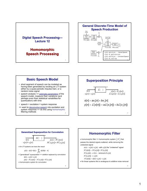
Digital Speech Processing
Processing—
Lecture 12
Homomorphic
Speech Processing
Basic Speech Model
• short segment of speech can be modeled as
having been generated by exciting an LTI system
either by a quasi-periodic impulse train, or a
random noise signal
• speech analysis => estimate parameters of the
speech h model, d l measure th their i variations i ti ( (and d
perhaps even their statistical variabilites-for
quantization) with time
• speech = excitation * system response
=> want to deconvolve speech into excitation and
system response => do this using homomorphic
filtering methods
Generalized Superposition for Convolution
x[ n]
*
H { }
*
y[ n]
= H { x[
n]
}
x1[ n]
∗ x2[
n]
H { x1[ n]
} ∗H
{ x2[
n]
}
• for LTI systems we have the result
yn [ ] = xn [ ] ∗ hn [ ] = xkhn [ ] [ −k]
∞
∑
k =−∞
• "generalized" superposition => addition replaced by convolution
xn [ ] = x1[ n] ∗x2[
n]
yn [ ] = H { x[ n]} = H { x1[ n]} ∗H
{ x2[
n]}
• homomorphic system for
convolution
1
3
5
General Discrete Discrete-Time Time Model of
Speech Production
pL[ n] = p[ n] ∗hV[ n]
−− Voiced Speech
hV[ n] = AV ⋅g[ n] ∗v[ n] ∗r[
n]
pL[ n] = u[ n] ∗hU[ n]
−− Unvoiced Speech
hU[ n] = AN ⋅v[ n] ∗r[
n]
2
Superposition Principle
+ +
x[ n]
x 1[
n]
+ x2[
n]
L{
}
y[ n]
= L{
x[
n]}
L { x1[ n]
} + L{
x2[
n]
}
xn [ ] = ax1[ n] + bx2[ n]
y[ n] = L{ x[ n]} = aL{ x [ n]} + bL{ x [ n]}
1 2
Homomorphic Filter
• homomorphic filter => homomorphic system ⎡
⎣H⎤ ⎦ that
passes the desired signal unaltered, while removing the
undesired signal
x ( n ) = x 1 1[ n] ∗ x 2 2[ n] - with x 1 1[
n]
the "undesired" signal g
H { xn [ ]} = H { x1[ n]} ∗H{
x2[ n]}
H { x1[ n]} → δ(
n) - removal of x1[ n]
H { x2[ n]} → x2[ n]
H { xn [ ]} = δ[
n] ∗ x2[ n] = x2[ n]
• for linear systems this is analogous to additive noise removal
4
6
1

x[ n]
x n x n
Canonic Form for Homomorphic
Deconvolution
* + + + + *
D ∗{
} L{
}
−1
D { }
xˆ[ n]
yn ˆ[ ] ∗ yn [ ]
ˆ[ ] ˆ [ ]
ˆ [ ] ˆ [ ]
1[ ] ∗ 2[
] x1 n + x2 n y1 n + y2 n
1 ∗ 2
y [ n] y [ n]
• any homomorphic system can be represented as a cascade
of three systems, e.g., for convolution
1. system takes inputs combined by convolution and transforms
them into additive outputs
2. system is a conventional linear system
3. inverse of first system--takes additive inputs and transforms
them into convolutional outputs
Properties of Characteristic
Systems
xn ˆ[ ] = D∗{ xn [ ]} = D∗{
x1[ n] ∗x2[
n]}
= D∗{ x1[ n]} + D∗{
x2[ n]}
= x xˆ [ n ] + x xˆ [ n ]
1 2
D ˆ D ˆ ˆ
{ y [ n]} { y [ n]}
−1 ∗ { yn [ ]} =
−1
∗ { y1[ n] + y2[ n]}
−1 = D∗ ˆ1 −1
∗D∗
ˆ2
= y1[ n] ∗ y2[ n] = y[ n]
Canonic Form for Deconvolution Using DTFTs
• need to find a system that converts convolution to addition
xn [ ] = x1[ n] ∗x2[
n]
jω jω jω
Xe ( ) = X1( e ) ⋅X2(
e )
• since
D { [ ]} ˆ ˆ ˆ
∗ xn = x1[ n] + x2[ n] = xn [ ]
⎡ jω ( ) ⎤ ˆ jω ˆ jω ˆ jω
D∗
Xe = X1( e ) + X2( e ) = Xe ( )
⎣ ⎦
=> use log function which
converts products to sums
ˆ jω ( ) log ⎡ jω ( ) ⎤ log ⎡ jω jω
Xe = Xe = X1( e ) ⋅ X2( e ) ⎤
⎣ ⎦ ⎣ ⎦
log ⎡ jω 1( ) ⎤ log ⎡ jω ˆ ˆ
2( ) ⎤ jω jω
= X e + X e = X1( e ) + X2( e )
⎣ ⎦ ⎣ ⎦
ˆ jω ( ) ⎡ ˆ jω ˆ jω ˆ ω ˆ ω
1( ) 2( ) ⎤ j j
Ye = L X e + X e = Y1( e ) + Y2( e )
⎣ ⎦
jω ( ) exp ˆ jω = ˆ j
Ye ⎡ ω
Y1( e ) + Y2( e ) ⎤ jω jω
= Y1( e ) ⋅Y2(
e )
⎣ ⎦
7
9
Canonic Form for Homomorphic Convolution
x[ n]
x n x n
* + + + + *
D ∗{
} L{
}
−1
D { }
xˆ[ n]
yn ˆ[ ] ∗ yn [ ]
ˆ ˆ
ˆ ˆ
1[ ] ∗ 2[
] x1[ n] + x2[ n]
y1[ n] + y2[ n]
1 ∗ 2
y [ n] y [ n]
xn [ ] = x 1 [ n ] ∗ x 2 [ n ]
- convolutional relation
xn ˆ[ ] = D ˆ ˆ
∗{
xn [ ]} = x1[ n] + x2[ n]
- additive relation
yn ˆ[ ] = L{
xˆ ˆ ˆ ˆ
1[ n] + x2[ n]} = y1[ n] + y2[ n]
- conventional linear system
−1
y[ n] = D { ˆ ˆ
∗ y1[ n] + y2[ n]} = y1[ n] ∗y2[
n]
- inverse of convolutional relation
=> design converted back to linear system, L
D∗
⎡⎣ ⎤⎦
- fixed (called the characteristic system for homomorphic deconvolution)
−1
D∗ ⎡⎣ ⎤⎦
- fixed (characteristic system for inverse homomorphic deconvolution)
Discrete Discrete-Time Time Fourier
Transform Representations
p
Characteristic System for
Deconvolution Using DTFTs
jω ∞
∑
n=−∞
− jωn Xe ( ) = xne [ ]
ˆ jω jω jω jω
Xe ( ) = log ⎡
⎣
Xe ( ) ⎤
⎦
= log Xe ( ) + jarg ⎡
⎣
Xe ( ) ⎤
⎦
π
1 ˆ jω jωn xn ˆ[ ] = ( ) ω
2π
∫ Xe e d
−π
8
10
12
2

Inverse Characteristic System for Deconvolution Using
DTFTs
jω ∞
∑
n=−∞
− jωn Ye ˆ( ) = yne ˆ[
]
jω ( ) exp ˆ jω
Ye = ⎡ ( ) ⎤
⎣
Ye
⎦
π
1
jω jωn yn [ ] = ( ) ω
2π
∫ Ye e d
−π
Problems with arg Function
13
{ (
jω ) } ≠ { 1(
jω
) }
jω
+ ARG { X 2 ( e ) }
ARG X e ARG X e
jω jω
{ Xe } = { X1e }
jω
+ arg { X2( e ) }
arg ( ) arg ( )
Complex and Real Cepstrum
define the inverse Fourier transform of ˆ jω
•
Xe ( ) as
π
1
ˆ[ ] ˆ jω jωn xn = ( ) ω
2π
∫ Xe e d
−π
• where xn ˆ[
] called the "complex cepstrum" since a complex
logarithm g is involved in the computation
• can also define a "real
cepstrum" using just the real part of
the logarithm, giving
π
1
[ ] Re ⎡ ˆ jω ( ) ⎤ jωn cn =
ω
2π
∫ Xe e d
⎣ ⎦
−π
π
1
jω jωn = log | ( ) | ω
2π
∫ Xe e d
−π
• can show that cn [ ] is the even part of xn ˆ[
]
15
17
Issues with Logarithms
• it is essential that the logarithm obey the equation
log ⎡ jω jω 1( ) 2( ) ⎤ log ⎡ jω 1( ) ⎤ log ⎡ jω
X e ⋅ X e = X e + X2( e ) ⎤
⎣ ⎦ ⎣ ⎦ ⎣ ⎦
jω jω
• this is trivial if X1( e ) and X2( e ) are real -- however usually
jω jω
X1( e ) and X2( e ) are complex
• on the unit circle the complex log can be written in the form:
arg ⎡ jω
( ) ⎤
jω jω
j X e
Xe ( ) = | Xe ( )| e ⎣ ⎦
log ⎡ jω ( ) ⎤ ˆ jω ω ω
( ) log ⎡ j
= = | ( )| ⎤+ arg ⎡ j
Xe Xe Xe j Xe ( ) ⎤
⎣ ⎦ ⎣ ⎦ ⎣ ⎦
• no problems with log magnitude term; uniqueness
problems
arise in defining the imaginary part of the log; can show that
the imaginary part (the phase angle of the z-transform) needs
to be a continuous odd function of ω
Complex Cepstrum Properties
i Given a complex logarithm that satisfies the phase continuity
condition, we have:
π
1
jω jω jωn xn ˆ[ ] = (log | X( e ) | jarg{ X( e )}) e dω
2π
∫
+
−π
jω jω
i If xn [ ] real, then log|X ( e ) | is an even function of ω and arg{ X( e )}
is an odd function of ω.
This means that the real and imaginary parts of
the complex log have the appropriate symmetry for xn ˆ[ ] to be a real
sequence, and xn ˆ[ ] can be represented as:
xn ˆ[ ] = cn [ ] + dn [ ]
jω
where cn [ ] is the inverse DTFT of log |X ( e )| and the even part of xn ˆ[
], and
jω
dn [ ] is the inverse DTFT of arg{ Xe ( )} and the odd part of xn ˆ[
]:
xn ˆ[ ] + xˆ[ −n] xn ˆ[ ] −xˆ[ −n]
cn [ ] = ; dn [ ] =
2 2
Terminology
• Spectrum – Fourier transform of signal autocorrelation
• Cepstrum – inverse Fourier transform of log spectrum
• Analysis – determining the spectrum of a signal
• Alanysis – determining the cepstrum of a signal
• Filtering – linear operation on time signal
• Liftering – linear operation on cepstrum
• Frequency – independent variable of spectrum
• Quefrency – independent variable of cepstrum
• Harmonic – integer multiple of fundamental frequency
• Rahmonic – integer multiple of fundamental frequency
14
16
18
3

z-Transform Transform Representation
i The z − transform of the signal:
xn [ ] = x1[ n]* x2[ n]
is of the form:
X( z) = X1( z) ⋅X2(
z)
i With an appropriate definition of the complex log, we get:
X Xˆ ( z ) = log{ X ( z )} = log{ X X1 ( z ) ⋅ X X2 ( z )}
= log{ X1(
z)} + log{ X2( z)}
= Xˆ ( z) + Xˆ ( z)
1 2
Inverse Characteristic System for
Deconvolution
∞
∑
Yz ˆ( ) = ynz ˆ[
]
n=−∞
−n
[ ]
Yz ( ) = exp ⎡ ˆ(
) ⎤
⎣
Yz
⎦
= log Yz ( ) + jarg Yz ( )
1
n
yn [ ] = ( )
2π
∫ Yzzdz
j
z-Transform Transform Cepstrum Alanysis
i express X( z)
as product of minimum-phase and
maximum-phase signals, i.e.,
i where
X( z) = X ( z) ⋅z
X ( z)
min
max
−M
0
min max
M
i
− 1
∏ ( 1−
k )
A az
X ( z)
=
k = 1
N
i
−1
∏(
1−
cz k )
k = 1
i all poles and zeros inside unit circle
Mi
Mi
−1
∏(
) k ∏
X ( z) = −b
1−bz
k = 1
k = 1
i all zeros outside unit circle
( )
k
19
21
23
Characteristic System for Deconvolution
∞
−n
Xz ( ) = ∑ xnz [ ] =
n=−∞
jarg { X( z)
}
Xz ( ) e
Xˆ ( z) = log X( z) = log X( z) + jarg X( z)
[ ] [ ]
1 ˆ n
xn ˆ[ ] = ( )
2π
∫ X z zdz
j
z-Transform Transform Cepstrum Alanysis
• consider digital systems with rational z-transforms of the general type
Xz ( ) =
M
M
A a z b z
i
0
−1 ∏( 1− k ) ∏(
1−
−1 −1)
k
k= 1 k=
1
Ni
−1
∏(
1−
cz k )
k = 1
i we can express the above equation as:
M0MiM0 −M0 −1 −1
z A∏−b 1− 1−
k ∏ akz ∏ bkz k= 1 k = 1
k=
1
Xz ( ) =
Ni
−1
∏(
1−
cz k )
k = 1
• with all coefficients ak, bk, ck < 1 => all ck
poles and
ak zeros are inside the unit circle; all bk
zeros
are outside the unit circle;
( ) ( ) ( )
z-Transform Transform Cepstrum Alanysis
i can express xn [ ] as the convolution:
xn [ ] = xmin[ n] ∗xmax[ n−M0] i minimum-phase component is causal
x [ n ] = 0, , n<
0
min
i maximum-phase component is anti-causal
x [ n] = 0, n>
0
max
M0
factor z is the shift in time ori
−
i gin by M 0
samples required so that the overall sequence,
xn
[ ] be causal
20
22
24
4

z-Transform Transform Cepstrum Alanysis
• the complex logarithm of Xz ( ) is
( ) log ⎡⎣ ( ) ⎤⎦
log |
M0
| ∑log
|
k = 1
−1
k |
−M0
log[ ]
M M
N
Xz ˆ = Xz = A + b + z +
i 0
i
− 1 − 1
∑ ∑log ( 1− az k ) + ∑ ∑log ( 1−bz k ) − ∑ ∑log
( 1−cz
k )
k= 1 k= 1 k=
1
• evaluating Xz ˆ ( ) on the unit circle we can ignore the term
0
related to log ⎡ jωM e ⎤ (as this contributes only to the imaginary
⎣ ⎦
part and is a linear phase shift)
Cepstrum Properties
1. complex cepstrum is non-zero and of infinite extent for
both positive and negative n, even though x[ n]
may be
causal, or even of finite duration ( X( z)
has only zeros).
2. complex cepstrum is a decaying sequence that is bounded by:
| n|
α
| xn ˆ[
]| < β , for | n|
→∞
| n |
3. zero-quefrency value of complex cepstrum (and the cepstrum)
depends on the gain constant and the zeros outside the unit circle.
Setting x ˆ[0] = 0 (and therefore c[0]
= 0)
is equivalent to normalizing
the log magnitude spectrum to a gain constant of:
M0
−1
A∏( − bk)
= 1
k = 1
4. If X( z) has no zeros outside the unit circle (all bk=
0), then:
xn ˆ[ ] = 0, n<
0 (minimum-phase
signals)
5. If X( z) has no poles or zeros inside the unit circle (all ak, ck
= 0), then:
xn ˆ[ ] = 0, n>
0 (maximum-phase signals)
z-Transform Transform Cepstrum Alanysis
• Example 2--consider
the case of a digital system with a
single zero outside the unit circle ( b < 1)
x2( n) = δ( n) + bδ( n+
1)
X2 ( z ) = 1 + bz (zero at z =− 1 / b )
ˆ
2( ) = log [ 2(
) ] = log(
1+
)
∞ + 1
( −1)
= ∑ ( )
= 1
ˆ2
n
X z bz z b
X z X z bz
n n
b z
n n
n+ 1 n
( −1)
b
x ( n) = u( −n−1) n
25
27
29
z-Transform Transform Cepstrum Alanysis
• we can then evaluate the remaining terms, use power series
expansion for logarithmic terms (and take the inverse
transform to give the complex cepstrum) giving:
π
1
ˆ(
) ˆ jω jωn xn = ( ) ω
2π
∫ Xe e d
2π
∫
−π
∞ n
Z
log(1 − Z) =− ∑ , | Z | < 1
n=
1 n
M0
−1
= log | A | + ∑log
| bk| k = 1
n = 0
Ni n Mi
n
ck ak
= ∑ −
n ∑ n
k= 1 k=
1
n > 0
M0 −n
bk
= ∑ n
k = 1
n < 0
26
z-Transform Transform Cepstrum Alanysis
i The main z-transform formula for cepstrum alanysis is based on
the power series expansion:
∞ ( −1)
∑
n+
1
n
log( 1+ x) = x x < 1
n=
1 n
i EExample l 1
--Apply A l thi this fformula l tto th the exponential ti l sequence
n
1
x1( n)
= aun ( ) ⇔ X1( z)
= −1
1−
az
n+
1
∞
ˆ −1( −1)
n −n
X1( z) = log[ X1( z)] = −log( 1−
az ) = −∑( −a)
z
n=
1 n
n ∞ n
a 1
ˆ 1( ) ( 1) ˆ
− ⎛a ⎞ −n
x n = u n− ⇔ X1( z) = −log( 1−
az ) = ∑⎜
⎟z
n n=
1 ⎝ n ⎠
z-Transform Transform Cepstrum Alanysis for 2 Pulses
• Example 3--an
input sequence of two pulses of the form
x3( n) = δ( n) + αδ( n− Np)
( 0 < α < 1)
−Np
X3( z) = 1+
αz
ˆ
−Np
X3( z) = log ⎡⎣X3( z) ⎤⎦
= log(
1+
αz
)
∞ n + 1
( −1)
n −nNp
= ∑ α z
n
n=
1
∞
k
ˆ k + 1 α
x3( n) = ∑(
−1) δ ( n−kNp) k
k = 1
• the cepstrum is an impulse train with impulses spaced at p samples
N
N p
2N 2Np 3N 3Np 28
30
5

Cepstrum for Train of Impulses
• an important special case is a train of impulses
of the form:
∑ M
xn ( ) = αδ(
n−rN) r p
r = 0
M
N
α
0
−rNp
∑ r
r =
Xz ( ) = z
−Np −1
• clearly Xz ( ) is a polynomial in z rather than z ;
thus Xz ( ) can be expressed as a product of factors
−Np
Np
of the form ( 1−az ) and ( 1−bz
), giving a complex
cepstrum, xn ˆ(
), that is non-zero only at integer multiples of N
z-Transform Transform Cepstrum Alanysis for
Convolution of 3 Sequences
i Example 5--consider
the convolution of sequences 1, 2 and 3, i.e.,
x5( n) = x1( n) ∗x2( n) ∗x3(
n)
n
= ⎡
⎣
aun ( ) ⎤
⎦
∗ [ δ( n) + bδ( n+ 1)
] ∗ ⎡
⎣δ( n) + αδ(
n−N) ⎤ p ⎦
n n−N p n
n− N p + 1
α p α
p
= a u ( n ) + a u ( n n− N ) + ba u ( n n+ 1 ) + ba u ( n n− N + 1 )
i The complex cepstrum is therefore the sum of the complex cepstra
of the three sequences
xˆ5( n) = xˆ1( n) + xˆ ˆ
2( n) + x3( n)
n ∞ k+ 1 k n+ 1 n
a ( −1) α ( −1)
b
= un ( − 1) + ∑ δ ( n− kNp) + u( −n−1) n k n
k = 1
Homomorphic Analysis of
Speech Model
p
31
33
35
z-Transform Transform Cepstrum Alanysis for
Convolution of 2 Sequences
--consider the convolution of sequences 1 and 3, i.e.,
4( ) 1( ) 3(
) ( ) δ( ) αδ(
)
( ) α ( )
The comple cepstr m is therefore the s mofthecomple
−
i Example 4
n
x n = x n ∗ x n = ⎡
⎣
a u n ⎤
⎦
∗ ⎡
⎣ n + n−N ⎤ p ⎦
n
n Np
= aun + a un−Np i The complex cepstrum is therefore the sum of the complex
cepstra
of the two sequences (since convolution in the time domain is
converted to addition in the cepstral domain)
xˆ ( n) = xˆ ( n) + xˆ ( n)
4 1 3
n ∞ k+ 1 k
a ( −1)
α
= un ( − 1)
+ ∑ δ ( n−kNp) n k
k = 1
Example: a=.9, b=.8, a=.7, Np=15
( 1)
+
− b
n
n 1 n
a
n
n
∞
∑
k = 1
32
( 1 α )
−Np
( 1+
bz)
Xz ( ) = + z
−1
( 1−
az )
k+ 1 k
( −1)
α
δ [ n−kNp] k
Homomorphic Analysis of Speech Model
• the transfer function for voiced speech is of the form
HV( z) = AV ⋅G(
z) V( z) R( z)
i with effective impulse response for voiced speech
h hV [ n ] = A AV ⋅ g [ n ] ∗ v [ n ] ∗ r [ n ]
• similarly for unvoiced speech we have
H U ( z) = AU⋅V( z) R( z)
i with effective impulse response for unvoiced speech
h [ n] = A ⋅v[ n] ∗r[
n]
U U
34
36
6

Complex Cepstrum for Speech
• the models for the speech components are as follows:
Mi
M0
−M−1 ∏ 1− k ∏ 1−
k
k= 1 k=
1
Ni
−1
∏(
1−
cz k )
k = 1
a k = b k = 0
Az ( a z ) ( b z)
1. vocal tract: Vz ( ) =
--for o voiced o ced speec speech, , oonly y po poles es => a b , aall
k
--unvoiced speech and nasals,
need pole-zero model but all poles are
inside the unit circle => ck
< 1
--all speech has complex poles and zeros that occur in complex conjugate
pairs
−1
2. radiation model: Rz ( ) ≈1−z(high frequency emphasis)
3. glottal pulse model: finite duration pulse with transform
Li
L0
−1
Gz ( ) = B∏( 1−αkz) ∏(
1−βkz)
k= 1 k=
1
with zeros both inside and outside the unit circle
Simplified Speech Model
• short-time speech model
x[ n] = w[ n] ⋅ p[ n] ∗g[ n] ∗v[ n] ∗r[
n]
≈ pw [ n ] ∗ h hv [ n ]
• short-time complex cepstrum
xn ˆ[ ] = pˆ [ n] + gn ˆ[ ] + vn ˆ[
] + rn ˆ[
]
w
[ ]
Time Domain Analysis
37
39
41
Complex Cepstrum for Voiced
Speech
• combination of vocal tract, glottal pulse and
radiation will be non-minimum phase =>
complex cepstrum exists for all values of n
• the complex cepstrum will decay rapidly for
large n (due to polynomial terms in expansion
of complex cepstrum)
• effect of the voiced source is a periodic pulse
train for multiples of the pitch period
Analysis of Model for Voiced Speech
i Assume sustained /AE/ vowel with fundamental frequency of 125 Hz
i Use glottal pulse model of the form:
⎧0.5
[1 − cos( π ( n+ 1) / N1)] 0 ≤n≤ N1−1
⎪
gn [ ] = ⎨cos(0.5
π ( n+ 1 −N1)/ N2) N1 ≤n≤ N1+ N2
−2
⎪
⎩ 0
otherwise
N1 = 25, N2
= 10
⇒ 34 sample impulse response, with transform
33 33
−33 −1
Gz ( ) = z ∏( −bk ) ∏(1
−bz k ) ⇒ all roots outside unit circle ⇒ maximum phase
k= 1 k=
1
i Vocal tract system specified by 5 formants (frequencies and bandwidths)
1
V( z)
= 5
−2πσ kT −1 −4πσ
kT
−2
∏(1−
2e cos(2 π FT k ) z + e z )
k = 1
{ F , σ } = [(660,60),(1720,100),(2410,120),(3500,175),(4500,250)]
k k
i Radiation load is simple first difference
−1
( ) 1 , 0.96
Rz = − γzγ =
Pole Pole-Zero Zero Analysis of Model
Components
38
40
42
7

Spectral Analysis of Model
Complex Cepstrum of Model
i The voiced speech signal is modeled as:
xn [ ] = AV ⋅gn [ ] ∗vn [ ] ∗rn [ ] ∗pn
[ ]
i with complex cepstrum:
sn ˆ[ ] = log| A | [ ] ˆ[ ] ˆ[ ] ˆ[ ] ˆ
V δ n + gn + vn + rn + pn [ ]
i glottal pulse is maximum phase ⇒ gn ˆ[ [ ] = 00, n > 0
i vocal tract
and radiation systems are minimum phase
⇒ vn ˆ[ ] = 0, n< 0, rn ˆ[
] = 0, n<
0
∞ k
ˆ −N β
p −kNp
Pz ( ) =−log(1 − β z ) = ∑ z
k = 1 k
∞ k
β
pn ˆ[ ] = ∑ δ[
n−kNp] k
k = 1
Resulting Complex and Real
Cepstra
43
45
47
Speech Model Output
Cepstral Analysis of Model
Frequency Domain Representations
44
46
48
8

Frequency
Frequency-Domain Domain Representation of
Complex Cepstrum
Inverse System- System DFT Implementation
Cepstral Computation Aliasing
49
51
N=256, N Np=75, =75,
α=0.8 =0.8
Circle dots are
are
cepstrum
values in
correct
locations; all
other dots are
results of
aliasing due to
finite range
computations
53
The Complex Cepstrum-DFT Cepstrum DFT Implementation
2π j k
N
∞
∑
n n=−∞∞
2π
− j kn
N
Xk [ ] = Xe ( ) = xne [ ] k= 01 , ,..., N−1,
jω
i Xp[ k] is the N point DFT corresponding to X( e )
Xk ˆ[ ] = Xe ˆ(
) = log Xk [ ] = log Xk [ ] + jarg Xk [ ]
j2πk/ N { } { }
N−1
∑ ˆ
2π
j kn
N
∞
∑
01 1
1
xn ˆ[
] = Xke [ ] = xn ˆ[
+ rN] n= , ,..., N−
N k= 0
r=−∞
• x ˆ[
n] is an aliased version of xˆ[ n]
⇒use
as large a value of N as possible to minimize aliasing
The Cepstrum-DFT Cepstrum DFT Implementation
π
1
jω jωn cn [ ] = log| ( )| ω
2π
∫ Xe e d −∞ < n<
∞
−π
i Approximation to cepstrum using DFT:
2π 2π
j k
∞
− j kn
N N
Xk [ ] = Xe ( ) = ∑ xne [ ] k= 01 , ,..., N−1,
n=−∞
N −1
1
j2πkn/ N
cn [
] = ∑log|
Xk [ ]| e , 0≤ n≤N−1 N k = 0
∞
cn (
) = ∑ cn [ + rN] n= 01 , ,..., N−1
r =−∞
• cn [
] is an aliased version of cn [ ] ⇒use
as large a value of N
as possible to minimize aliasing
ˆ[ ] + ˆ
xn x[ −n]
cn ( ) =
2
Summary
1. Homomorphic System for Convolution:
z( ) log( ) L( ) exp( ) z-1 ^ ^ x[n] X(z) X(z)
Y(z)
Y(z)
y[n]
( )
X(z)
^
z-1 ( )
x[n] ^
Linear
System
y[n] ^
z( )
Y(z)
^
2. Practical Case:
z( ) → DFT
−1
z () → IDFT
jω
jω jω
jarg { X( e ) }
Xe ( ) = Xe ( ) e
jω jω jω
log ⎡
⎣
Xe ( ) ⎤
⎦
= log Xe ( ) + jarg Xe ( )
{ }
50
52
54
9

Summary
3. Complex Cepstrum:
1 ˆ jω jωn xn ˆ[
] = ( ) ω
2 ∫ Xe e d
44. CCepstrum: t
π
π −π
π
1
jω jωn cn [ ] = log ( ) ω
2π
∫ Xe e d
−π
xn ˆ[ ] + xˆ[ −n]
cn [ ] = = even part of xn ˆ[
]
2
Complex Cepstrum Without Phase
Unwrapping
i short-time analysis uses finite-length windowed segments, x[ n]
M
−n
th
X( z) = ∑ x[ n] z , M -order polynomial
n=
0
i Find polynomial roots
Mi ∏
M0
−1 m ∏
−1 −1
m
m= 1 m=
1
X( z) = x[0] (1 −a z ) (1 −b
z )
i am
roots are inside unit circle (minimum-phase
part)
i bm
roots are outside unit circle (maximum-phase part)
−1 −1
i Factor out terms of form − bmz giving:
MiM0 −M 0
−1
X( z) = Az (1 −a z ) (1 −b
z)
m m
m= 1 m=
1
M0
M0
−1
∏ m
m=
1
A= x[0]( −1)
b
∏ ∏
i Use polynomial root finder
to find the zeros that lie inside
and outside the unit circle and solve directly for xn ˆ[ ] .
Recursive Relation for Complex
Cepstrum for Minimum Phase Signals
• the complex cepstrum for minimum phase signals
can be computed recursively from the input signal,
xn ( ) using the relation
ˆ( ) = 0 < 0
= log ⎡⎣ ( 0) ⎤⎦
= 0
−1
( ) ⎛ ⎞ ( − )
= − ˆ( )
0
( 0) ∑⎜ ⎟
>
⎝ ⎠ ( 0)
n
xn n
x n
xn k xn k
xk n
x n x
k = 0
55
57
59
x(n)
Summary
~
X(k X(k) ^ ^
X(k X(k)
x(n x(n)
DFT Complex Log IDFT
5. Practical Implementation of Complex Cepstrum:
∞
j( 2π/ N) k − j( 2π/
N) kn
Xk [ ] = Xe ( ) = ∑ xne [ ] )
n=−∞
X ˆ [ k] = log { Xp( k) } = log Xp( k) + jarg { Xp( k)
}
N−1∞
1 ˆ j( 2π
/ N
ˆ ) kn
xn [ ] = ∑Xke [ ] = ∑ xn ˆ[
+ rN]
⇒aliasing
N k= 0
r=−∞
xn ˆ[ ] = aliased version
of xn ˆ[
]
6. Examples:
∞ r
1
a
Xz ( ) = ⇔ xn ˆ[
] = δ [ ]
−1
∑ n−r 1−
az r = 1 r
∞ r
b
Xz ( ) = 1−bz⇔
xn ˆ[
] = − ∑ δ [ n+ r]
r = 1 r
Cepstrum for Minimum Phase Signals
• for minimum phase signals (no poles or zeros outside unit circle) the complex cepstrum
can be completely represented by the real part of the Fourier transforms
• this means we can represent the complex
cepstrum of minimum phase signals by the log
of the magnitude of the FT alone
• since the real part of the FT is the FT of the even part of the sequence
ˆ
ˆ( ) ˆ(
)
Re ⎡ jω ⎡ + − ⎤
( ) ⎤
xn x n
Xe = FT
⎣ ⎦ ⎢
2
⎥
⎣ 2 ⎦
jω
FT ⎡⎣c( n)
⎤⎦
= log Xe ( )
xn ˆ( ) + xˆ( −n)
cn ( ) =
2
• giving
xn ˆ(
) = 0 n<
0
= cn ( ) n=
0
= 2cn ( ) n>
0
• thus the complex cepstrum (for minimum phase signals) can be computed by computing
the cepstrum and using the equation above
58
Recursive Relation for Complex
Cepstrum for Minimum Phase Signals
xn ( ) ←⎯→ Xz ( ) 1. basic z-transform
dX( z)
nx( n) ←⎯→− z =−zX′
( z) dz
2. scale by n rule
xn ˆ( ) ←⎯→ Xz ˆ ( ) = log [ Xz ( ) ] 3. definition of complex cepstrum
dXˆ ( z) d X′ ( z)
= [ log[ Xz ( )] ] =
dz dz X( z)
4. differentiation of z-transform
dXˆ ( z)
−z
Xz ( ) =−zX′
( z)
dz
5. multiply both sides of equation
56
60
10

Recursive Relation for Complex
Cepstrum for Minimum Phase Signals
dXˆ ( z)
nxˆ( n) ∗x( n) ←⎯→− z X( z) =−zX′ ( z) ←⎯→ nx( n)
dz
∞
nx( n) = xˆ ( k) x( n −k)
k
∑
k =−∞
( )
i for minimum phase systems we have xn ˆ(
) = 0for n<
0,
xn ( ) = 0 for n < 0 0,
giving:
n
( ) ˆ
⎛k⎞ xn = ∑ xkxn ( ) ( −k) ⎜ ⎟
k = 0
⎝n⎠ i separating out the term for k = n we get:
n−1
ˆ
⎛k⎞ xn ( ) = ∑ xkxn ( ) ( − k) ⎜ ⎟+
x( 0)
xn ˆ(
)
k = 0
⎝n⎠ n−1
xn ( ) xn ( − k) ˆ( ) ˆ
⎛k⎞ xn = − ∑ xk ( ) , > 0
( 0) = 0 ( 0)
⎜ ⎟ n
x k x ⎝n⎠ xˆ( 0) = log x( 0) , xˆ( n) = 0, n < 0
[ ]
Cepstrum for Maximum Phase Signals
• for maximum phase signals (no poles or
zeros inside unit circle)
xn ˆ( ) + xˆ( −n)
cn ( ) =
2
• giving
xn ˆ(
) = 0 n>
0
= cn ( ) n=
0
= 2cn ( ) n<
0
• thus the complex cepstrum (for maximum
phase signals) can be computed
by computing
the cepstrum and using the equation above
Computing Short-Time
Short Time
Cepstrums from Speech
U Using i Polynomial P l i l Roots R t
61
63
65
Recursive Relation for Complex
Cepstrum for Minimum Phase Signals
i why is xˆ( 0) = log[ x(
0)]?
i assume we have a finite sequence xn ( ), n= 01 , ,..., N−1
i we can write xn ( ) as:
xn ( ) = x( 0) δ( n) + x( 1) δ( n− 1) + ... + xN ( −1) δ(
N−1)
⎡ x() 1 x( N −1)
⎤
= x( 0) ⎢δ( n) + δ( n− 1) + ... + δ(
N −1)
⎣ x( 0) x(
0)
⎥
⎦
i taking z − transforms, we get:
N−1
NZ1 NZ 2
−n−1 Xz ( ) = ∑ xnz ( ) = G∏( 1−az k ) ∏(
1−bz
k )
n= 0 k= 1 k=
1
i where the first term is the gain, G = x(
0),
and the two product terms are the
zeros inside and outside the
unit circle.
i for minimum phase systems we have all zeros inside the unit circle so the
second product term is gone, and we have the result that
xˆ( 0) = log[ G] = log[ x( 0)]; xˆ( n) = 0, n < 0
NZ1 a
xn ˆ( ) =
0
k=1
n ⎛ ⎞ k − ∑⎜
⎟ n >
⎝ n ⎠
Recursive Relation for Complex
Cepstrum for Maximum Phase Signals
• the complex cepstrum for maximum phase signals
can be computed recursively from the input signal,
xn ( ) using the relation
xn ˆ( ) = 0 n>
0
= log ⎡⎣x( 0) ⎤⎦
n = 0
xn ( )
= −
x( 0) 0
⎛k⎞ xn ( − k)
∑ ⎜ ⎟xk
ˆ( )
⎝n⎠ x(
0)
n<
0
k= n+
1
Cepstrum From Polynomial Roots
62
64
66
11

Cepstrum From Polynomial Roots
Practical Considerations
• window to define short-time analysis
• window duration (should be several pitch
periods long)
•size i of f FFT (to (t minimize i i i aliasing) li i )
• elimination of linear phase components
(positioning signals within frames)
• cutoff quefrency of lifter
• type of lifter (low/high quefrency)
Voiced Speech Example
67
69
Hamming window
40 msec duration
(section beginning
at sample 13000
in file
test_16k.wav)
71
Computing Short-Time
Short Time
Cepstrums from Speech
Using the DFT
Computational Considerations
Voiced Speech Example
68
70
wrapped phase
unwrapped
phase
72
12

Voiced Speech Example
Complex Cepstrum of Speech
• model of speech:
– voiced speech produced by a quasi-periodic
pulse train exciting slowly time-varying linear
system y => p[n] p[ ] convolved with hv[n] v[ ]
– unvoiced speech produced by random noise
exciting slowly time-varying linear system =>
u[n] convolved with hv[n] • time to examine full model and see what
the complex cepstrum of speech looks like
Voiced Speech Example
73
75
Cepstrally
smoothed log
magnitude, 50
quefrencies
cutoff
Cepstrally
unwrapped
phase, 50
quefrencies
cutoff
77
Characteristic System for
Homomorphic Convolution
• still need to define (and design) the L
operator part (the linear system
component) p ) of the system y to completely p y
define the characteristic system for
homomorphic convolution for speech
– to do this properly and correctly, need to look
at the properties of the complex cepstrum for
speech signals
Homomorphic Filtering of Voiced
Speech
• goal is to separate out the
excitation impulses from the
remaining components of the
complex cepstrum
• use cepstral window, l(n), to
separate excitation pulses from
combined vocal tract
– l(n)=1 for |n|

Voiced Speech Example
High quefrency
liftering; cutoff
quefrency=50;
log magnitude
and unwrapped
phase
Unvoiced Speech Example
79
Hamming window
40 msec duration
(section beginning
at sample 3200 in
file test_16k.wav)
Unvoiced Speech Example
81
83
Voiced Speech Example
Estimated
excitation
function for
voiced speech
(Hamming
window
weighted)
Unvoiced Speech Example
80
wrapped phase
unwrapped
phase
Unvoiced Speech Example
82
Cepstrally
smoothed log
magnitude, 50
quefrencies
cutoff
Cepstrally
unwrapped
phase, 50
quefrencies
cutoff
84
14

Unvoiced Speech Example
Estimated
excitation source
for unvoiced
speech section
(Hamming
window
weighted)
Review of Cepstral Calculation
• 3 potential methods for computing cepstral
coefficients, xn ˆ[ ] , of sequence x[n]
– analytical method; assuming X(z) is a rational
function; find poles and zeros and expand using log
power series i
– recursion method; assuming X(z) is either a minimum
phase (all poles and zeros inside unit circle) or
maximum phase (all poles and zeros outside unit
circle) sequence
– DFT implementation; using windows, with phase
unwrapping (for complex cepstra)
Cepstral Computation Aliasing
i Effect of quefrency aliasing via a simple example
xn [ ] = δ[ n] + αδ[
n−Np] i with discrete-time Fourier transform
j ( ) ω
j N
X e 1 e ω
α −
= +
p
i We can express the complex logarithm as
ˆ j
j Np
X( e ) log{1 e }
ω
ω
α −
∞ m+ 1 m ⎛( −1)
α ⎞
= + = ∑⎜
⎟e
m=
1⎝
m ⎠
i giving a complex cepstrum in the form
∞ m+ 1 m ⎛ ⎞
( −1)
α
xn ˆ[ ] = ∑⎜
⎟δ[
n−mNp] m=
1⎝
m ⎠
− jωmNp 85
87
89
Short Short-Time Time Homomorphic Analysis
STFT
Example 11—single
single pole sequence
(computed using all 3 methods)
[ ] = [ ]
n
xn aun
n
a
xn ˆ[ ] = un [ −1]
n
Example 22—voiced
voiced speech frame
86
88
90
15

Example 33—low
low quefrency liftering
Example 4—effects 4 effects of low quefrency lifter
Example 66—phase
phase unwrapping
91
93
95
Example 33—high
high quefrency liftering
Example 55—phase
phase unwrapping
Homomorphic Spectrum Smoothing
92
94
96
16

Running Cepstrum
Running Cepstrums
Cepstrum Distance Measures
i The cepstrum forms a natural basis for comparing
patterns in speech recognition or vector quantization
because of its stable mathematical characterization
for speech signals
i A typical "cepstral distance
measure" is of the form:
nco
2
D = ([] cn −cn
[])
∑
n=
1
where cn [ ] and cn [ ] are cepstral sequences corresponding
to frames of signal, and D is the cepstral distance between
the pair of sequences.
i Using Parseval's theorem, we can express the cepstral
distance in the frequency domain as:
1 π
jω jω
2
D (log | H( e ) | log | H( e ) |) dω
2π
π
Thus we see that the cepstral distance is actually a log
magnitude spe
−
= ∫
−
i
ctral distance
97
99
101
Running Cepstrum
Cepstrum Applications
Mel Frequency Cepstral Coefficients
i Basic idea is to compute a frequency analysis based on a filter
bank with approximately critical band spacing of the filters and
bandwidths. For 4 kHz bandwidth, approximately 20 filters are used.
i First perform a short-time Fourier analysis, giving Xm[ k], k = 0,1,..., NF / 2
where m is the frame number and k is the frequency index (1 to half
the size of the FFT)
i Next the DFT values are grouped g p together g in critical bands and weighted g
by triangular weighting functions.
98
100
102
17

Mel Frequency Cepstral Coefficients
th th
i The mel-spectrum of the m frame for the r filter ( r = 1, 2,..., R)
is defined as:
Ur
1
2
MFm[]
r = ∑ | Vr[] k Xm[]| k
Ar
k= Lr
th
where Vr[ k] is the weighting function for the r filter, ranging from
DFT index Lr to Ur,
and
U Ur
2
Ar = ∑ | Vr[ k]|
k= Lr
th
is the normalizing factor for the r mel-filter. (Normalization guarantees
that if the input spectrum is flat, the mel-spectrum is flat).
i A discrete cosine transform of the log magnitude of the filter outputs is
computed to form the function mfcc [ n]
as:
R 1 ⎡2π⎛ 1⎞
⎤
mfccm[ n] = ∑log(
MFm[
r]) cos r n , n 1,2,..., Nmfcc
R
⎢ ⎜ + ⎟
r=
1
R 2
⎥ =
⎣ ⎝ ⎠ ⎦
i Typically N = 13 and R=
24 for 4 kHz bandwidth speech signals. 103
mfcc
Homomorphic Vocoder
• time-dependent complex cepstrum retains all the
information of the time-dependent Fourier
transform => exact representation of speech
• time dependent real cepstrum loses phase
information -> > not an exact representation of
speech
• quantization of cepstral parameters also loses
information
• cepstrum gives good estimates of pitch, voicing,
formants => can build homomorphic vocoder
Homomorphic Vocoder
• l(n) is cepstrum window that selects low-time
values and is of length 26 samples homomorphic
vocoder
105
107
Delta Cepstrum
i The set of mel frequency cepstral coefficients provide perceptually
meaningful and smooth estimates of speech spectra, over time
i Since speech is inherently a dynamic signal, it is reasonable to seek
a representation that includes some aspect of the dynamic nature of
the time derivatives (both first and second order derivatives) of the shortterm
cepstrum
i The resulting parameter sets are called the
delta cepstrum (first derivative)
and the delta-delta cepstrum (second derivative).
i Th The simplest i l t method th d of f computing ti ddelta lt cepstrum t parameters t is i a first fi t
difference of cepstral vectors, of the form:
Δ mfccm[ n] = mfccm[ n] −mfccm−1[
n]
i The simple difference is a poor approximation to the first derivative and is
not generally used. Instead a least-squares approximation to the local slope
(over a region
around the current sample) is used, and is of the form:
M
∑ k( mfccm+
k[
n])
k=−M Δ mfccm[
n]
=
M
2
∑ k
k=−M where the region is M frames before and after the current frame
Homomorphic Vocoder
1. compute cepstrum every 10-20 msec
2. estimate pitch period and
voiced/unvoiced decision
3. quantize and encode low-time cepstral
values l
4. at synthesizer-get approximation to hv(n) or hu(n) from low time quantized cepstral
values
5. convolve hv(n) or hu(n) with excitation
created from pitch, voiced/unvoiced, and
amplitude information
Homomorphic Vocoder Impulse Responses
104
106
108
18

Summary
• Introduced the concept of the cepstrum of a signal,
defined as the inverse Fourier transform of the log of the
signal spectrum
1
j
ˆ[ ] log ( )
xn F X e ω
− = ⎡
⎣
⎤
⎦
• Showed cepstrum p reflected pproperties p of both the
excitation (high quefrency) and the vocal tract (low
quefrency)
– short quefrency window filters out excitation; long quefrency
window filters out vocal tract
• Mel-scale cepstral coefficients used as feature set for
speech recognition
• Delta and delta-delta cepstral coefficients used as
indicators of spectral change over time 109
19