An Efficient Algorithm for Fractal Analysis of Textures - Decom

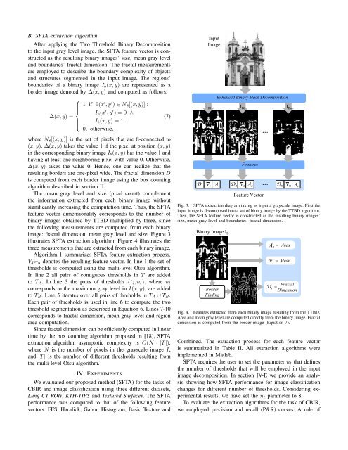
B. SFTA extraction algorithm
After applying the Two Threshold Binary Decomposition
to the input gray level image, the SFTA feature vector is constructed
as the resulting binary images’ size, mean gray level
and boundaries’ fractal dimension. The fractal measurements
are employed to describe the boundary complexity of objects
and structures segmented in the input image. The regions’
boundaries of a binary image Ib(x, y) are represented as a
border image denoted by ∆(x, y) and computed as follows:
⎧
⎪⎨
∆(x, y) =
⎪⎩
1 if ∃(x ′ , y ′ ) ∈ N8[(x, y)] :
Ib(x ′ , y ′ ) = 0 ∧
Ib(x, y) = 1,
0, otherwise.
where N8[(x, y)] is the set of pixels that are 8-connected to
(x, y). ∆(x, y) takes the value 1 if the pixel at position (x, y)
in the corresponding binary image Ib(x, y) has the value 1 and
having at least one neighboring pixel with value 0. Otherwise,
∆(x, y) takes the value 0. Hence, one can realize that the
resulting borders are one-pixel wide. The fractal dimension D
is computed from each border image using the box counting
algorithm described in section II.
The mean gray level and size (pixel count) complement
the information extracted from each binary image without
significantly increasing the computation time. Thus, the SFTA
feature vector dimensionality corresponds to the number of
binary images obtained by TTBD multiplied by three, since
the following measurements are computed from each binary
image: fractal dimension, mean gray level and size. Figure 3
illustrates SFTA extraction algorithm. Figure 4 illustrates the
three measurements that are extracted from each binary image.
Algorithm 1 summarizes SFTA feature extraction process.
VSFTA denotes the resulting feature vector. In line 1 the set of
thresholds is computed using the multi-level Otsu algorithm.
In line 2 all pairs of contiguous thresholds in T are added
to TA. In line 3 the pairs of thresholds {ti, nl}, where nl
corresponds to the maximum gray level in I(x, y), are added
to TB. Line 5 iterates over all pairs of threholds in TA ∪ TB.
Each pair of thresholds is used in line 6 to compute the two
threshold segmentation as described in Equation 6. Lines 7-10
corresponds to fractal dimension, mean gray level and region
area computation.
Since fractal dimension can be efficiently computed in linear
time by the box counting algorithm proposed in [18], SFTA
extraction algorithm asymptotic complexity is O(N · |T |),
where N is the number of pixels in the grayscale image I,
and |T | is the number of different thresholds resulting from
the multi-level Otsu algorithm.
IV. EXPERIMENTS
We evaluated our proposed method (SFTA) for the tasks of
CBIR and image classification using three different datasets,
Lung CT ROIs, KTH-TIPS and Textured Surfaces. The SFTA
performance was compared to that of the following feature
vectors: FFS, Haralick, Gabor, Histogram, Basic Texture and
(7)
Input
Image
Enhanced Binary Stack Decomposition
I B1 I B2 I Bn
Features
Feature Vector
...
...
D1 v1 A1 D2 v2 A2 Dn vn An
Fig. 3. SFTA extraction diagram taking as input a grayscale image. First the
input image is decomposed into a set of binary image by the TTBD algorithm.
Then, the SFTA feature vector is constructed as the resulting binary images’
size, mean gray level and boundaries’ fractal dimension.
Binary Image I B
Border
Finding
A 1 =
v 1
D 1
Area
= Mean
Fractal
=
Dimension
Fig. 4. Features extracted from each binary image resulting from the TTBD.
Area and mean gray level are computed directly from the binary image. Fractal
dimension is computed from the border image (Equation 7).
Combined. The extraction process for each feature vector
is summarized in Table II. All extraction algorithms were
implemented in Matlab.
SFTA requires the user to set the parameter nt that defines
the number of thresholds that will be employed in the input
image decomposition. In section IV-E we provide an analysis
showing how SFTA performance for image classification
changes for different number of thresholds. Considering experimental
results, we have set the nt parameter to 8.
To evaluate the extraction algorithms for the task of CBIR,
we employed precision and recall (P&R) curves. A rule of