An Efficient Algorithm for Fractal Analysis of Textures - Decom
An Efficient Algorithm for Fractal Analysis of Textures - Decom
An Efficient Algorithm for Fractal Analysis of Textures - Decom

Create successful ePaper yourself
Turn your PDF publications into a flip-book with our unique Google optimized e-Paper software.
Method<br />
Name<br />
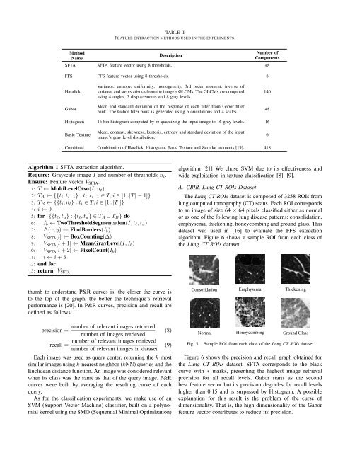
TABLE II<br />
FEATURE EXTRACTION METHODS USED IN THE EXPERIMENTS.<br />
Description<br />
Number <strong>of</strong><br />
Components<br />
SFTA SFTA feature vector using 8 thresholds. 48<br />
FFS FFS feature vector using 8 thresholds. 8<br />
Haralick<br />
Gabor<br />
Variance, entropy, uni<strong>for</strong>mity, homogeneity, 3rd order moment, inverse <strong>of</strong><br />
variance and step statistics from the image’s GLCMs. The GLCMs are computed<br />
using 4 angles, 5 displacements and 8 gray levels.<br />
Mean and standard deviation <strong>of</strong> the response <strong>of</strong> each filter from Gabor filter<br />
bank. The Gabor filter bank is generated using 6 orientations and 4 scales.<br />
Histogram 16 bin histogram computed by re-quantizing the input image to 16 gray levels. 16<br />
Basic Texture<br />
Mean, contrast, skewness, kurtosis, entropy and standard deviation <strong>of</strong> the input<br />
image’s gray level distribution.<br />
Combined Combination <strong>of</strong> Haralick, Histogram, Basic Texture and Zernike moments [19]. 418<br />
<strong>Algorithm</strong> 1 SFTA extraction algorithm.<br />
Require: Grayscale image I and number <strong>of</strong> thresholds nt.<br />
Ensure: Feature vector VSFTA.<br />
1: T ← MultiLevelOtsu(I, nt)<br />
2: TA ← {{ti, ti+1} : ti, ti+1 ∈ T, i ∈ [1..|T | − 1]}<br />
3: TB ← {{ti, nl} : ti ∈ T, i ∈ [1..|T |]}<br />
4: i ← 0<br />
5: <strong>for</strong> {{tℓ, tu} : {tℓ, tu} ∈ TA ∪ TB} do<br />
6: Ib ← TwoThresholdSegmentation(I, tℓ, tu)<br />
7: ∆(x, y) ← FindBorders(Ib)<br />
8: VSFTA[i] ← BoxCounting(∆)<br />
9: VSFTA[i + 1] ← MeanGrayLevel(I, Ib)<br />
10: VSFTA[i + 2] ← PixelCount(Ib)<br />
11: i ← i + 3<br />
12: end <strong>for</strong><br />
13: return VSFTA<br />
thumb to understand P&R curves is: the closer the curve is<br />
to the top <strong>of</strong> the graph, the better the technique’s retrieval<br />
per<strong>for</strong>mance is [20]. In P&R curves, precision and recall are<br />
defined as follows:<br />
number <strong>of</strong> relevant images retrieved<br />
precision =<br />
number <strong>of</strong> images retrieved<br />
number <strong>of</strong> relevant images retrieved<br />
recall =<br />
number <strong>of</strong> relevant images in dataset<br />
Each image was used as query center, returning the k most<br />
similar images using k-nearest neighbor (kNN) queries and the<br />
Euclidean distance function. <strong>An</strong> image was considered relevant<br />
when its class was the same as that <strong>of</strong> the query image. P&R<br />
curves were built by averaging the resulting curve <strong>of</strong> each<br />
query.<br />
As <strong>for</strong> the classification experiments, we make use <strong>of</strong> an<br />
SVM (Support Vector Machine) classifier, built on a polynomial<br />
kernel using the SMO (Sequential Minimal Optimization)<br />
(8)<br />
(9)<br />
algorithm [21] We chose SVM due to its effectiveness and<br />
wide exploitation in texture classification [8], [9].<br />
A. CBIR, Lung CT ROIs Dataset<br />
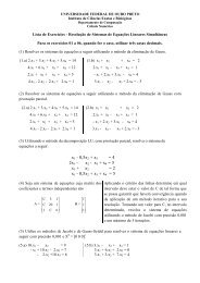
The Lung CT ROIs dataset is composed <strong>of</strong> 3258 ROIs from<br />
lung computed tomography (CT) scans. Each ROI corresponds<br />
to an image <strong>of</strong> size 64 × 64 pixels classified either as normal<br />
or as one <strong>of</strong> the following lung disease patterns: consolidation,<br />
emphysema, thickening, honeycombing and ground glass. This<br />
dataset was used in [16] to evaluate the FFS extraction<br />
algorithm. Figure 6 shows a sample ROI from each class <strong>of</strong><br />
the Lung CT ROIs dataset.<br />
140<br />
Consolidation Emphysema Thickening<br />
Normal Honeycombing Ground Glass<br />
Fig. 5. Sample ROI from each class <strong>of</strong> the Lung CT ROIs dataset<br />
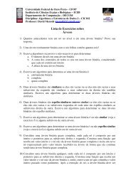
Figure 6 shows the precision and recall graph obtained <strong>for</strong><br />
the Lung CT ROIs dataset. SFTA corresponds to the black<br />
curve with ∗ marks, presenting the highest image retrieval<br />
precision <strong>for</strong> all recall levels. Gabor starts as the second<br />
best feature vector but its precision degrades <strong>for</strong> recall levels<br />
higher than 0.15 and is surpassed by Histogram. A possible<br />
explanation <strong>for</strong> this result is the problem <strong>of</strong> the curse <strong>of</strong><br />
dimensionality. That is, the high dimensionality <strong>of</strong> the Gabor<br />
feature vector contributes to reduce its precision.<br />
48<br />
6