The Gödel universe - Institut für Theoretische Physik der Universität ...

More documents

Recommendations

Info

Obviously, general solutions of the geodesic equations can be mapped onto other general solutions as well. Therefore, we consider arbitrary initial conditions as above and a desired destination position x µ 1 . The component x µ 0 is rotated around the z-axis until ϕ = π/2 is reached, isometrically translated along ξ µ 1 to map onto the desired radial coordinate r = xr 1, then rotated to the destination angular coordinate ϕ = x ϕ 1 , and finally isometrically translated in time and the z-coordinate to arrive at x µ . Again, the initial direction is only rotated 1 due to the Killing vector field ξ µ 1 by an angle F(˜η1), where ˜η1 = ln r2 1 + r2 G /2 + r1 r2 1 + r2 G r2 0 + r2 G /2 + r0 r 2 0 + r 2 G . (42) Numerical implementations of this procedure and the general solution to the geodesic equations yield identical results. B. Mapping of the Gödel horizon Because Gödel’s universe is homogeneous, every observer O,A or B can legitimately declare his position as the origin of a coordinate system, where the line element takes the form of eq. (1). This definition yields an equivalent formulation of the Gödel horizon. Fig. 4 indicates how these horizons are shaped. The Gödel horizon around any point is the convex hull of all lightlike geodesics starting there. Furthermore, the horizon itself is a closed null curve (CNC), because ds 2 = 0 along the Gödel radius. We could use the general solution to the geodesic equations to calculate the exact shape. However, the usage of finite isometric transformations is by far more elegant. Due to the homogeneity of the spacetime, each observer states that ’his’ horizon is circular within the (xy)plane. 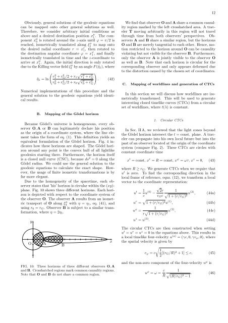Fig. 10 shows three different horizons. Each horizon is depicted with respect to the coordinate system of the observer O. The observer A results from an isometric transport of O along ξ µ 4 with η = η1, eq. (41), and using r0 = rG. Observer B is subject to a similar transformation, where η = 2η1. y O A B FIG. 10: Three horizons of three different observers O,A and B. Crosshatched regions mark common causality regions. Note that O and B do not share a common region. x 12 We find that observer O and A share a common causality region marked by the left crosshatched area. A traveler T moving arbitrarily in this region will not travel through time from both observers’ perspectives. Observers A and B share a similar region, but the horizons O and B are merely tangential to each other. Hence, motion restricted to the horizon around O can be causality violating but not visible for the observer B. Furthermore, only the observer A is jointly visible to the observer O as well as B. Note that each horizon is circular for the corresponding observer and only appears deformed due to the distortion caused by the chosen set of coordinates. C. Mapping of worldlines and generation of CTCs In this section we will discuss how worldlines are isometrically transformed. This will be used to generate interesting closed timelike curves (CTCs) from a circular set of worldlines, where t(λ) is constant. 1. Circular CTCs In Sec. II A, we reviewed that the light cones beyond the Gödel horizon intersect the t = const. plane. A traveler can propagate into his own local future but into the past of an observer located at the origin of the coordinate system (compare Fig. 2). These CTCs are circles with constant coordinate time x t = const, x r = R = const, x ϕ = ωτ, x z = 0, (43) where R ≥ rG. We generate CTCs when we require that ut is zero. To find the corresponding direction in the local frame of reference, eqns. (12), we transform a local vector to the coordinate representation: u t = 1 c u(0) √ 2r 1 − rGc 1 + (r/rG) 2 u(2) , (44a) u r = 1 + (r/rG) 2u (1) , (44b) u ϕ 1 = r 1 + (r/rG) 2 u(2) , (44c) u z = u (3) . (44d) The circular CTCs are then constructed when setting u t = u r = u z = 0 in the equations above. This results in a local timelike four-velocity u (a) = (γc,0,γvϕ,0), where the spatial velocity is given by 1 vϕ = c 2 [(rG/R) 2 + 1] ≤ c, (45) and the non-zero component of the four-velocity u µ is u ϕ = ω = c 1 R (R/rG) 2 . (46) − 1
Inserting the four-velocity into the Lagrangian, eq. (6), proves that this four-velocity is indeed a timelike vector. The four-acceleration is obtained using eq. (4), and the only non-zero component turns out to be a r = ω 2 R [(R/rG) 2 + 1][2(R/rG) 2 − 1] , (47) which is positive ∀R > rG. Hence, the traveler has to accelerate radially outwards to sustain the circular motion on the CTC. Note that there exists only one angular velocity ω for each radius R > rG to form a CTC. Other values of ω generate possible but non-closed worldlines. These worldlines are not causality violating and are comparable to the helix segment of the CTC in Fig. 2. From these results we calculate the Fermi-Walker transport of an arbitrary vector X µ , eq. (5), and obtain the coupled system of linear differential equations ˙X t (τ) = −X r √ 2 2R (λ) R2 − r2 G (R2 + r2 G ), (48a) ˙X r (τ) = X t √ 2 2 2 2 2c R (R + rG ) (λ) r2 G (R2 − r2 , (48b) G )3/2 ˙X ϕ (τ) = X r 2cR (λ) 2rG (R2 − r2 G )3/2 (R2 + r2 G ), (48c) ˙X z (τ) = 0. (48d) With the abbreviations R2 − r2 GrG B12 = − c(R2 + r2 , (49a) G ) √ 2 2rG B13 = (R2 + r2 G )R2 − r2 , (49b) G (49c) the integration yields X t (τ) = B12 [E2 cos(ντ) − E1 sin(ντ)] , (50a) X r (τ) = E2 sin(ντ) + E1 cos(ντ), (50b) X ϕ (τ) = B13 [E2 cos(ντ) − E1 sin(ντ)] + E3, (50c) X z (τ) = E3λ, (50d) where √ 2 2cR ν = rG(r2 G − R2 . (51) ) Before determining the integration constants Ei, we formulate this solution with respect to a local comoving frame. First, eqns. (50) are expressed using the local rest frame, eqns. (12), denoted as X (a) . To transform this intermediate result into a local comoving frame, we only have to apply a Lorentz boost. Obviously, the traveler T is moving in the e (2)-direction of the rest frame. Hence, to transform the Fermi-Walker transported vector into the comoving frame of the moving observer T, we apply a Lorentz boost to X (a) (τ) in the same direction 13 with β = vϕ/c (compare eq. (45)). To express the fact that the comoving frame results from a Lorentz transformation Λ (a)(b) of the local rest frame, we designate the resulting vector as X (aΛ) . Then, the local initial conditions X (aΛ) (0) = X (aΛ) 0 fix the integration constants. The result of this calculation is X (0Λ) (τ) = X (0Λ) 0 , (52a) X (1Λ) (τ) = X (1Λ) 0 cos(ντ) + X (2Λ) 0 sin(ντ), (52b) X (2Λ) (τ) = −X (1Λ) 0 sin(ντ) + X (2Λ) 0 cos(ντ), (52c) X (3Λ) (τ) = X (3Λ) 0 . (52d) With these results at hand we consider the special case X (aΛ) 0 = (0,1,0,0) and calculate the rotation angle α after one orbit. After one period we have ωτ◦ = 2π and obtain τ◦ = 2πR (R/rG) c 2 − 1, (53a) α = ντ◦ = − 2√2π(R/rG) 3 (R/rG) 2 , (53b) − 1 where we have used ω from eq. (46) In the limit R → rG we obtain a closed null curve (CNC), where the spatial components describe the Gödel horizon. The local velocity of the corresponding photon, eq. (45), is c (as expected) and the proper time τ◦, eq. (53a), converges to zero. However, a photon has to be forced on a circular orbit, because this curve does not represent a geodesic. This could be achieved, e.g., using an appropriate arrangement of mirrors. 2. Mapping of CTCs This set of CTCs can now be mapped onto CTCs which pass through the origin. We transport a circular CTC along the Killing vector field ξ µ 4 , eq. (14c). Using an approach similar to the mapping of geodesics, Sec. VA, we calculate the isometric transformation of the point x µ = (t0,R,π,0) to the origin, arriving at the same curve parameter η1, eq. (41), which is now used in the solution to the equations of transport for ξ µ 4 , eqns. (31). The same transformation is applied to each point of the worldline. The resulting behavior can be anticipated when analyzing Fig. 8 and Fig. 9. The distance of lines of finite isometric transport, Fig. 8, decreases for larger distances to the origin. Hence, we expect that the transformed circle must appear deformed; resulting in a smaller radius of curvature for those parts of the worldline now distant from the origin. Fig. 9 reveals that the coordinate time values of one semi-cycle will be pushed to negative values while the other semi-cycle will experience a shift to positive values. This expected qualitative behavior is verified by the results shown in Fig. 11 and 12. Apparently, the results of the previous section, which have been formulated with respect to a local frame, are still valid.
Page 1 and 2: The Gödel universe: Exact geometri
Page 3 and 4: tation scalar ΩG = √ 2c , (2) m
Page 5 and 6: D. Killing vectors Solving the Kill
Page 7 and 8: y a) b) C A c) d) B ct ct ct A B =
Page 9 and 10: takes to travel from the horizon to
Page 11: Let x µ (λ) be an arbitrary light
Page 15 and 16: Acknowledgments We thank the DFG (G
Page 17 and 18: . Transformation of vectors The equ
Page 19: part of the geodesic lying beyond t

The Gödel universe - Institut für Theoretische Physik der Universität ...

Create successful ePaper yourself

Delete template?

Save as template?