The Gödel universe - Institut für Theoretische Physik der Universität ...

The Gödel universe:
Exact geometrical optics and analytical investigations on motion
Frank Grave, 1, 2, ∗ Michael Buser, 3 Thomas Müller, 2 Günter Wunner, 1 and Wolfgang P. Schleich 3
1 1. Institut für Theoretische Physik, Universität Stuttgart,
Pfaffenwaldring 57 // IV, 70550 Stuttgart, Germany
2 Visualisierungsinstitut der Universität Stuttgart,
Universität Stuttgart, Nobelstraße 15, D-70569 Stuttgart, Germany
3 Institut für Quantenphysik, Universität Ulm, D-89069 Ulm, Germany
(Dated: October 16, 2009)
In this work we derive the analytical solution of the geodesic equations of Gödel’s universe for
both particles and light in a special set of coordinates which reveals the physical properties of this
spacetime in a very transparent way. We also recapitulate the equations of isometric transport
for points and derive the solution for Gödel’s universe. The equations of isometric transport for
vectors are introduced and solved. We utilize these results to transform different classes of curves
along Killing vector fields. In particular, we generate non-trivial closed timelike curves (CTCs) from
circular CTCs. The results can serve as a starting point for egocentric visualizations in the Gödel
universe.
PACS numbers: 95.30.Sf, 04.20.-q, 04.20.Ex, 04.20.Fy, 04.20.Gz, 04.20.Jb
I. INTRODUCTION
Gödel’s cosmological solution of Einstein’s field equations,
published in 1949 [1], represents a basic model
of a “rotating universe” with negative cosmological constant
Λ. Its spacetime curvature originates from a homogeneous
matter distribution which rotates around every
point with a constant rotation rate. The energy momentum
tensor consists of an ideal fluid whose pressure and
mass density are connected to the cosmological constant
and the rotation scalar of Gödel’s universe [2].
A particularly puzzling feature of Gödel’s universe is
the existence of closed timelike curves (CTCs). Gödel
himself was the first who pointed out their existence
within the framework of general relativity, although the
van Stockum dust cylinder model of 1937 already possesses
CTCs [3]. Besides Gödel’s universe and the van
Stockum dust cylinder, numerous other spacetimes have
been found, which allow for time travel, such as the Kerr
metric [4], the Gott universe of two cosmic strings [4, 5],
various wormhole spacetimes [6], or two massive particles
in a (2 + 1)-dimensional anti-de-Sitter spacetime [7].
Over the last decades, these metrics stimulated many discussions
on the philosophical consequences of time travel
and causality violations within the theory of relativity. In
particular, Hawking established the so-called chronology
protection conjecture which states that the laws of nature
prevent time travel on all but sub-microscopic scales [8].
Gödel’s metric facilitates analytical investigations, because
it is highly symmetric and possesses five independent
Killing vector fields. Already Gödel himself took
advantage of four isometry groups to show that his cos-
∗ Electronic address: frank.grave@vis.uni-stuttgart.de;
URL: http://www.vis.uni-stuttgart.de/~grave
APS/123-QED
mological solution is spacetime homogeneous [1]. A more
detailed examination of the Killing fields was later performed
by Navez [9]. He showed that Gödel’s universe is
endowed with five independent Killing vector fields and
he examined the structure of the corresponding Lie algebra.
The Killing equations for Gödel-type spacetimes
were also discussed by Raychaudhuri et. al. [10]. They
derived the necessary conditions for Gödel-type metrics
to inherit at least four independent Killing vector
fields – constituting the minimum requirement to satisfy
the homogeneity of the spacetime. Based upon this
work, and independent of Naves’ work [9], Rebouças et.
al. [11] showed that these conditions lead to five independent
Killing vector fields. We note that Barrow and
Tsagas [12] investigated the stability of Gödel’s solution
with respect to scalar, vector, and tensor perturbation
modes using a gauge covariant formalism.
Gödel’s universe is one of the simplest solutions of Einstein’s
field equations which allows for CTCs. As pointed
out by Gödel [1] there exist geometrically very simple
CTCs corresponding to “circular orbits” in specific coordinates
which display the rotational symmetry of the
metric most clearly. These circular orbits were also discussed
by Raychaudhuri et. al. [10] and Pfarr [13], who
categorized them into CTCs, coordinate dependent pasttraveling
curves (PTCs) and closed null curves (CNCs).
Rosa and Letelier [14] analyzed the stability of CTCs under
tiny changes of the energy momentum tensor. However,
these circular orbits are not the only possible CTCs
in Gödel’s universe, see e. g. Sahdev et. al. [15].
The geodesic equations for Gödel’s metric have been
examined in several works so far. They were first solved
in 1956 by Kundt [16], who took advantage of the Killing
vectors and the corresponding constants of motion. In
1961, Chandrasekhar and Wright [17] presented an independent
derivation of the solution. They concluded that
there are no closed timelike geodesics and noted that this

fact seems to be contrary to Gödel’s statement that the
“circular orbits” allow one “to travel into the past, or
otherwise influence the past”. Nine years later, Stein [18]
pointed out that the “circular orbits” of Gödel are by no
means geodesics and that Chandrasekhar’s and Wright’s
conclusion was incorrect, see also [19]. Other detailed
studies of the geodesics in Gödel’s universe followed by
Pfarr [13] and Novello et. al. [20]. The latter provided a
detailed discussion on geodesical motion using the effective
potential as well as the analytical solution. They already
assumed that any geodesic can be generated from
geodesics starting at the origin by a suitable isometric
transformation.
The understanding of null geodesics provides the
bedrock for ray tracing in Gödel’s spacetime. Egocentric
visualizations of certain scenarios in Gödel’s universe can
be found in our previous work [21]. There, we presented
improvements for visualization techniques regarding general
relativity. Furthermore, finite isometric transformations
were used to visualize illuminated objects. This
method was technically reworked and improved in [22]
and resulted in an interactive method for visualizing various
aspects of Gödel’s universe from an egocentric perspective.
In that work, we used the analytical solution
to the geodesic equations and a numerical integration of
the equations of isometric transport.
This paper is organized as follows. In Sec. II A, we
review several basic characteristics of Gödel’s universe
to make this work self-contained. The equations of motion
are summarized and the constants of motion are expressed
with respect to a local frame of reference. All
Killing vector fields are specified as well. We follow the
notation of Kajari et. al. [2] because we regard their
choice of a set of coordinates as highly suitable and easily
interpretable. Sec. III details the solution to the geodesic
equations for timelike and lightlike motion. After discussing
the special case of geodesics starting at the origin,
we introduce the general solution and explain under
which circumstances time travel on geodesics is possible.
In Sec. IV, we derive analytical expressions on finite
isometric transformations along Killing vector fields for
points as well as directions. All results are then used
in Sec. V to isometrically transform initial conditions
for geodesics to map the special solution of the geodesic
equations onto the general solution. Also, the Gödel horizon
is calculated for different observers at rest with respect
to the rotating matter and depicted for our choice
of coordinates. Finally, we carry out a detailed analysis of
circular CTCs and use finite isometric transformations to
generate a class of non-circular CTCs. In the appendix,
we describe several details on the solution to the geodesic
equations and equations of isometric transport for easier
reproduction of our results by the reader. The last section
in the appendix provides interesting estimates of our
results using astronomical data.
II. GÖDEL’S UNIVERSE
A. Basic properties
For the reader’s convenience we recapitulate a few basic
features of Gödel’s universe. For details we refer, e.g.,
to the work of Kajari et. al. [2] or Feferman [23]. The line
element of Gödel’s universe in cylindrical coordinates [2],
with the velocity of light c and the Gödel radius rG, reads
ds 2 = −c 2 dt 2 +
dr 2
1 + (r/rG) 2 + r2 1 − (r/rG) 2 dϕ 2
+dz 2 − 2√2r2c dtdϕ, (1)
rG
when using a positive signature of the metric tensor, i.e.
sign(gµν)=+2. This convention will be used throughout
the paper. Furthermore, initial conditions for positions
and directions are always denoted by a lower index of
zero, i.e. x µ (0) = x µ
0 and uµ (0) = u µ
Gödel’s universe describes [1] a homogeneous universe,
in which matter rotates everywhere clockwise with a constant
angular velocity relative to the compass of inertia.
It can easily be shown that, in this reference frame, massive
particles with zero initial velocity propagate only in
time. Hence, these cylindrical coordinates are corotating
with the matter.
rG
y
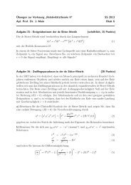
FIG. 1: Lightlike geodesics in the (xy)-subspace depicted in
pseudo-Cartesian coordinates (cf. Fig. 2 in [2]). Photons
emitted at the origin propagate counterclockwise into the future,
reach a maximum radial distance of rG, and then return
to the origin. It can be shown that there exists no causality
violation for arbitrary lightlike or timelike geodesics starting
at the origin.
The Gödel radius rG can be identified [2] with the ro-
0 .
x
2

tation scalar
ΩG =
√
2c
, (2)
making it inversely proportional to the angular velocity
of the rotating matter. Fig. 1 depicts several lightlike
geodesics starting at the origin. Photons reach the
Gödel radius, and their orbits are closed in the (xy)subspace
[33]. Thus rG constitutes an optical horizon
beyond which an observer located at the origin cannot
see, because photons starting with r0 > rG do not reach
the origin. Due to the stationarity of Gödel’s metric,
there exists no gravitational redshift; only Doppler shift
due to relative motion arises.
Comparable to asymptotic flat spacetimes, we can find
an interpretation for this set of coordinates. Because the
metric converges to the Minkowski metric of flat spacetime
(in cylindrical coordinates) for r → 0, we denote
this set as the coordinates of an observer resting at the
origin[34]. Coordinate time t and proper time τ of an
observer at the origin are identical. Hence, if we want to
make a statement on measurements performed by an observer,
it is very convenient if he rests at the origin. Due
to the homogeneity of Gödel’s universe we can transform
any physical situation in such a way that an arbitrary
observer is then located at the new origin. The mathematical
details are provided in Sec. IV.
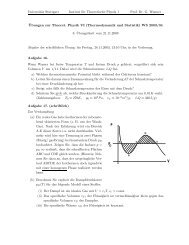
We denote an observer resting at the origin by O, other
resting observers by A,B,C and traveling observers (or
photons) by T. Fig. 2 illustrates a possible CTC. A traveler
T starts at the origin, accelerates beyond the horizon,
travels along a circular PTC into the past, reenters the
horizon, and then reaches the origin at the same coordinate
time of departure. The resulting curve is a noncircular
CTC. Time travel is only possible beyond the
horizon, because light cones intersect the plane of constant
coordinate time for all r > rG. Hence, a traveler
can travel into his own future but into the past of the
observer O.
The geodesic equations
rG
B. Equations of motion
¨x µ + Γ µ ρσ ˙x ρ ˙x σ = 0 (3)
govern the propagation of light or freely moving particles.
In this section, any derivative is with respect to an affine
parameter λ (for lightlike geodesics) or with regard to
proper time τ (for timelike motion). Because these equations
are of second order in λ or τ, respectively, initial
conditions for position and direction have to be specified.
If a massive particle is moving on an arbitrary timelike
worldline x µ (τ), a four-acceleration
a µ = ¨x µ + Γ µ ρσ ˙x ρ ˙x σ , (4)
FIG. 2: Chronological structure of Gödel’s universe. In this
xyt-diagram a possible timelike worldline is depicted. A traveler
T could move on this curve, propagating in his own local
future at any given point. Beyond the horizon (gray cylinder)
he travels into the past of an observer located at the origin.
The worldline itself is a CTC, because the traveler departs
from and returns to the origin at the same coordinate time t.
For an observer at the origin, coordinate time and proper time
coincide. The figure illustrates Gödel’s original idea to prove
that there exist CTCs through every point in spacetime [1].
must act on the particle. An arbitrary vector X along
this worldline (with tangent u µ ) will be Fermi-Walker
transported according to
0 = dXβ
1
c 2
dτ + Xγ u α Γ β αγ+
gγσu σ a β − gγσa σ u β X γ . (5a)
A vector on a geodesic will be parallel-transported using
a µ = 0 in the equations above.
To derive the equations of geodesical motion we here
use the Lagrangian formalism. The Lagrangian L =
3

gµνu µ u ν for Gödel’s metric (1) reads
L = −c 2 ˙t 2 +
˙r 2
1 + (r/rG) 2 + r2 1 + (r/rG) 2 ˙ϕ 2
+ ˙z 2 − 2√2r2c ˙t ˙ϕ. (6)
rG
Additionally, the constraint L = gµνu µ uν = κc2 has to
be fulfilled. The type of a geodesic is determined by the
parameter κ. For timelike geodesics we have κ = −1,
whereas lightlike geodesics require κ = 0.
Using the Euler-Lagrange equations of motion one
finds three constants of motion ki = ∂L/∂ ˙x i , where
√
2 2r
k0 = −c˙t − ˙ϕ, (7a)
rG
k2 = r 2 1 − (r/rG) 2 √
2 2r c
˙ϕ − ˙t, (7b)
rG
k3 = ˙z. (7c)
The quantities k0, k2 and k3 represent the conservation of
energy, angular momentum, and z-component of momentum,
respectively. These three constants can be solved
for ˙t, ˙ϕ and ˙z. Substituting the result of this calculation
in eq. (6), the Lagrangian becomes solely dependent on
r and ˙r. Using the constraint L(r, ˙r) = κc 2 we can solve
this equation for ˙r. We then obtain the equations of motion
for both photons and massive particles in the form
1 − (r/rG)
c˙t = −k0
2
√
2k2
−
1 + (r/rG) 2
rG [1 + (r/rG) 2 , (8a)
]
˙r 2 = (κc 2 − k 2 3) 1 + (r/rG) 2 − k2 2
+
r2 2 √ 2k0k2
+ k 2
0 1 − (r/rG) 2 , (8b)
rG
˙ϕ = k2 − √ 2r2k0/rG , (8c)
r 2 [1 + (r/rG) 2 ]
˙z = k3. (8d)
C. Initial conditions
Now, we will formulate the initial conditions of arbitrary
geodesics using the constants of motion. These initial
conditions will be expressed with respect to a local
frame of reference, because this formulation facilitates
statements on measurements done by arbitrary observers.
1. Local frame of reference
Any vector u can be expressed with respect to a particular
coordinate system or a local frame of reference
{e (a) : a = 0,1,2,3}, i.e.
u = u µ ∂µ = u (a) e (a). (9)
Greek indices denote vectors in coordinate representation,
whereas Latin indices in round brackets are used
for vectors expressed in a local frame. To obtain an orthonormal
system the condition
g(e (a),e (b)) := gµνe µ
(a) eν (b) = η (a)(b), (10a)
η (a)(b) = diag(−1,1,1,1), (10b)
has to be fulfilled, where the transformation matrices satisfy
4
e µ
(a) e(a)
ν = δ µ ν . (11)
We choose the local frame of reference of a static observer
– comoving with the rotating matter and resting with
respect to the cylindrical set of coordinates – and find
that
e (0) = 1
c ∂t, (12a)
e (1) = 1 + (r/rG) 2∂r, (12b)
1
e (2) =
r 1 + (r/rG) 2
√
2 2r
−
rGc ∂t
+ ∂ϕ , (12c)
e (3) = ∂z. (12d)
This tetrad, however, is not well-defined for r = 0. Because
the angular coordinate is undefined at r = 0,
we cannot formulate initial directions in ∂ϕ-direction.
Nevertheless we can exploit the rotational symmetry of
this spacetime. A geodesic can start with u ϕ
0
= 0 and
then be rotated around the z-axis afterwards to generate
geodesics starting at the origin and propagating in arbitrary
initial direction. Another possibility is to transform
the tetrad as well as the line element itself to Cartesian
coordinates to avoid the coordinate singularity in r = 0.
Unfortunately, Gödel’s universe loses its mathematical
elegance when considering a set of coordinates which is
not adjusted to the symmetries of the spacetime.
2. Local formulation of the constants of motion
We can express the constants of motion, eq. (7), with
respect to the chosen local frame of reference, eq. (12).
The result for both lightlike and timelike geodesics is
, (13a)
√
2 2r0 k0 = −u (0)
0
k2 = r0 1 + (r0/rG) 2u (2)
0 −
rG
u (0)
0 , (13b)
k3 = u (3)
0 . (13c)
The parameter r0 = r(0) is the initial radial coordinate of
the geodesic. Because any vector u = u (a) e (a) expressed
in a local system is treated like any vector in special relativity,
the sign of u (0)
0 determines whether the geodesic is
evolving into the future (+) or into the past (−). Hence,
k0 is associated with the time direction.

D. Killing vectors
Solving the Killing equations ξµ;ν+ξν;µ = 0 for Gödel’s
universe yields five Killing vector fields (cf. [2]), which
read
ξ µ
0 =
ξ µ
1
ξ µ
4
where
⎛
⎜
⎝
= 1
q(r)
⎞
1
0 ⎟
0
⎠ , ξ
0
µ
2 =
⎛
⎜
⎝
⎛
1 ⎜
= ⎜
q(r) ⎝
rG
2
rG
2r
− rG
rG
2r
⎛
⎜
⎝
⎞
0
0 ⎟
1
⎠ , ξ
0
µ
3 =
√r cos ϕ
2c
⎛
⎜
⎝
0
0
0
1
⎞
⎞
⎟
⎠ , (14a)
1 + (r/rG) 2 sinϕ
1 + 2(r/rG) 2 ⎟
cos ϕ ⎠ , (14b)
0
√r sin ϕ
2c
2 1 + (r/rG) 2 cos ϕ
1 + 2(r/rG) 2 ⎞
⎟
sin ϕ ⎠ ,
0
(14c)
q(r) = 1 + (r/rG) 2 . (15)
The first three Killing vectors (eq. (14a)) are trivial, corresponding
to the constants of motion (13), and represent
infinitesimal transformations in t, ϕ and z, respectively.
Eqns. (14b) and (14c) reveal that a radial transformation
generally affects time and angular coordinate as well.
Note that lower indices in Killing vectors serve to distinguish
different vector fields.
Taking advantage of the Killing vectors (14), the generators
of the corresponding Lie algebra read Xk =
ξ α k ∂/(∂xα ). In this representation the structure constants
Cijk follow from the Lie brackets [Xi,Xj] =
CijkXk according to
[X1,X2] = −[X2,X1] = −X4, (16a)
[X2,X4] = −[X4,X2] = −X1, (16b)
[X1,X4] = −[X4,X1] = 1
X0 + X2, (16c)
where [Xi,Xj] = XiXj − XjXi.
ΩG
(16d)
It is worthwhile noting that the set of generators defined
by L1 = X4, L2 = X1, L3 = −i(X2 + X0/ΩG) satisfies
the angular momentum algebra [Li,Lj] = iεijkLk,
as shown by Figuareido [24]. Here i,j,k ∈ {1,2,3} and
εijk represents the three-dimensional Levi-Cevita symbol.
Moreover, the remaining generators L0 = X0 and
L4 = X3 commute with L1, L2 and L3. This feature is
used e. g. in the analysis of the scalar wave equation in
Gödel’s Universe [24, 25].
III. SOLUTION TO THE GEODESIC
EQUATIONS
A. Geodesics for special initial conditions
In this section, we will present the solution of the
geodesic equations for special initial conditions. We consider
arbitrary timelike and lightlike geodesics starting at
the origin of the coordinate system. Lightlike geodesics
alone had been considered by Kajari et. al. [2]. Although
the general solution to the geodesic equations is introduced
in the next section, the special solution is necessary
to overcome the coordinate singularity in r = 0. In
principle, we could obtain the special solution from the
general solution by applying the limit r0 → 0 for the
initial radial coordinate r0. Unfortunately, this limit is
complicated to calculate.
The constants of motion, eq. (13), simplify for
geodesics starting at the origin. In particular, k2 vanishes,
and the equations of motion now read
using the abbreviations
1 − (r/rG)
c˙t = −k0
2
, (17a)
1 + (r/rG) 2
˙r 2 = K+ − K−(r/rG) 2 , (17b)
5
˙ϕ =
− √ 2k0
rG [1 + (r/rG) 2 ,
]
(17c)
˙z = k3, (17d)
K+ = κc 2 + k 2 0 − k 2 3, (18a)
K− = −κc 2 + k 2 0 + k 2 3. (18b)
Solving these equations is straightforward and outlined
in Sec. A1a. The solution reads
t(λ) = k0
√
2rG
λ + ϕ1(λ) + p1/2(λ) c c
+ t0, (19a)
K+
r(λ) = rG sin B1λ , (19b)
with
K−
ϕ(λ) = ϕ1(λ) + p 1/2(λ) − p0(λ) + ϕ0, (19c)
z(λ) = k3λ, (19d)
√B1
pq(λ) = πσ0 λ + q , (20a)
π
√
k0 2
ϕ1(λ) = arctan tan −
K−
B1λ
, (20b)
where we used the constant B1 from eq. (21a) and the
abbreviation for the initial temporal direction σ0 (cf.
eq. (22a)). The expression ⌊y⌋ is the mathematical floor
function, which ensures the continuous differentiability
of the solution, except for r = 0. As stated at the end of

Sec. II C1, we cannot directly generate geodesics starting
in the ∂ϕ-direction due to the coordinate singularity of
the cylindrical coordinate system. This coordinate singularity
is avoided by interpreting the integration constant
ϕ0 as the local starting direction in the (xy)-plane. For
ϕ0 = 0, the geodesic starts in positive x-direction if the
particle propagates into the future, i.e. k0 < 0. On the
other hand ϕ0 = π/2 results in a geodesic starting in
negative y-direction for k0 > 0. Note that the special solution
of the geodesic equations, eqns. 19, generalize the
results of the work of Kajari et. al. [2]. Setting k3 = 0
and κ = 0 reproduces their results regarding lightlike
motion in the (xy)-subspace.
a) z
b) ct
rG
x
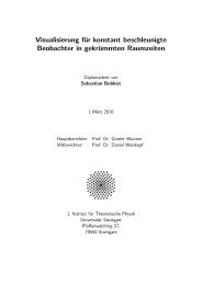
FIG. 3: Lightlike geodesics starting at the origin. For better
orientation, the Gödel horizon and three planar geodesics
(compare Fig. 1) are provided in Fig. 3a. The non-planar
geodesics are solid, dashed or densely dotted curves. The
angle between neighboring geodesics is 10 ◦ . Fig. 3b: Radial
coordinate as a function of coordinate time. Non-planar
geodesics do not reach the Gödel radius. Timelike geodesics
are of similar shape but reach smaller maximal radial distances
from the origin.
Fig. 3 depicts several geodesics with non-zero initial
velocity in e (3)-direction. Those geodesics do not reach
the Gödel horizon. However, the optical Gödel horizon is
of cylindrical shape, because geodesics with u (3) = ǫ with
ǫ ≪ 1 (almost planar geodesics) come arbitrarily close to
the horizon for sufficiently small ǫ. These geodesics still
reach any z-value after an appropriate number of cycles.
Timelike geodesics also do not reach the horizon when
starting from the origin, even in the planar case. Both
effects are caused by the radial solution, eq. (17b), where
the prefactor becomes K+/K− < 1. Fig. 3b shows that
geodesics starting at the origin do not violate causality –
with respect to the observer O – because dt/dλ ≥ 0.
B. Geodesics for arbitrary initial conditions
We will now discuss the general solution to the geodesic
equations for timelike and lightlike motion. For this task,
the full geodesic equations (8) for arbitrary initial conditions,
eqns. (13), have to be solved. An outline of the
y
rG
r
derivation is provided in Sec. A1b. We use the abbreviations
B1 = K−
r2 , B2 = −
G
k2 2
r4 , B3 =
G
K+
r2 +
G
2√2k0k2 r3 ,
G
(21a)
B4 = (rG/2) 2K2 + + K+( √ 2rGk0k2 + k2 2 ), (21b)
C1 = 1
2 √ 4 rGB3 − 2r
arcsin
B1
2
0K−
, (21c)
2rGB4
where the constants K+ and K− are identical to those
defined in eqns. (18). To distinguish radially outgoing or
incoming initial conditions as well as the initial temporal
direction of a geodesic, we use the signum functions
6
σ0 = sgn(u (0)
0 ), (22a)
σ1 = sgn(u (0)
1 ). (22b)
The integration constant C1 of the radial equation (8b)
is determined via r(0) = r0. Furthermore, we introduce
the auxiliary functions
v(λ) = B1(−σ1λ + C1),
σ1r
ϕ2(λ) = arctan
(23a)
2 G
2 √ B1(k2 + √ 2rGk0) ×
(2B1 + B3)tan(v(λ)) − B2
3 + 4B1B2
,
σ1r 2 G
(23b)
ϕ3(λ) = arctan
2 √
×
B1k2
B3 tan(v(λ)) − B2
3 + 4B1B2
, (23c)
˜p(λ) = πσ1σ0
√B1 π (σ1λ − C1) + 1
, (23d)
2
where the function ˜p(λ) ensures the continuous differentiability
of the solution and is analogous to eq. (20a) of
the special solution. Finally, the analytical solutions for
both arbitrary timelike and lightlike geodesics are found
in the form
t(λ) = k0
√
2rG
λ + [ϕ2(λ) + ˜p(λ)] + C3, (24a)
c
c
r
r(λ) = rG
3 GB3/2 − B4 sin(2v(λ))
, (24b)
rGK−
ϕ(λ) = ϕ2(λ) − ϕ3(λ) + C2, (24c)
z(λ) = k3λ + z0. (24d)
The integration constants C2 and C3 can be specified
by ϕ(0) = ϕ0 and t(0) = t0. If the geodesic is only
directed along the local e (3)-axis, i.e. u (1)
0 = u(2) 0 ≡ 0, we

y
a) b)
C
A
c)
d)
B
ct
ct
ct
A
B = rG
FIG. 4: Planar lightlike geodesics resulting from the general
analytical solution to the geodesic equations. In Fig. 4a, nine
geodesics at different initial positions are shown. Position A is
at r0 = rG/2, position B shows geodesics starting on the horizon
rG, and in C we have r0 = 3rG/2. At each starting point
geodesics propagate in +e(1)- or ±e(2)-direction, respectively.
Non-planar geodesics show a behavior similar to the special
solution, Fig. 3, i. e. are smaller in radial extent. Figs. 4b-d
show the radial coordinate of the geodesics as a function of
coordinate time.
obtain straight lines parallel to the z-axis, where t(λ) =
k0λ/c + t0.
In Fig. 4, several planar lightlike geodesics are depicted.
Fig. 4a shows the projection onto the (xy)subspace
and Fig. 4b-d display the correlation between
radial coordinate and coordinate time t. Most photons
in Fig. 4 partially travel back through time. This travel
through time is in most cases restricted to regions beyond
the Gödel horizon and therefore not measurable by the
observer O. Fig. 4b, in which several geodesics starting
at r0 = rG/2 are depicted, reveals an exception. The
magnified square shows that the corresponding photon
reenters the Gödel horizon before crossing it.
To investigate how far a traveler T can travel into the
past of an observer O, we use the general solution to
the geodesic equations (24). We consider an arbitrary
initial position and any initial direction within the local
{e (1),e (2)}-subspace. It can be shown that u (3)
0 must be
zero to maximize time travel [35]. Solving the radial so-
C
r
x
r
r
lution, eq. (24b), with respect to the curve parameter results
in an infinite number of solutions due to the periodicity
of r(λ). We choose the first two solutions λ1 (where
the photon or massive particle arrives at the horizon) and
λ2 (where it reappears from beyond the horizon). Inserting
λ1 and λ2 into the time solution, eq. (24a), yields a
difference in coordinate time
∆t = t(λ2) − t(λ1). (25)
Again, coordinate time and proper time of an observer
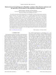
O are identical. Fig. 5 shows the result of these considerations.
In Fig. 5a, the minimal time difference ∆t,
eq. (25), is depicted for a given initial radial coordinate
r0. We find these values by numerically searching the
angle ξ0 for fixed r0, where ∆t becomes minimal. The
local angle between the starting direction and the e (1)axis
is denoted as ξ0. The correlation between ξ0 and r0
is shown in Fig. 5b. Radii ρ1,...,ρ5 denote certain initial
positions for the lightlike case, which we will now discuss.
We set ρ1 = rG/4, ρ2 = rG/2, ρ3 = rG, ρ4 ≈ 1.4rG, and
ρ5 ≈ 1.7rG. Obviously, time travel is only possible for
r0 ρ5.
Fig. 5a reveals that there exists a maximum time
travel (i.e. minimal ∆t with ∆t < 0) for a given initial
velocity. In the time travel region (0 ≤ r0 ≤ ρ5
in the lightlike case), ∆t appears constant for a large
region of initial radii (ρ1 ≤ r0 ≤ ρ4). Unfortunately,
equation (25) is too complicated to treat it analytically
despite its simple structure. Analytical investigations
are restricted to special cases, and for a detailed analysis
in general we have to resort to numerical investigations.
We find that ∆t is constant up to at least within
10 −10 in the region ρ1 ≤ r0 ≤ ρ4. The global minimum
can be estimated with ∆t(r0 = ρ2,ξ0), because
(d∆t(r0 = ρ2,ξ0))/(dξ0) ≡ 0 (exactly) for ξ0 = 0. The
global minimum ∆T c min = ∆t(r0 = ρ2,ξ0) then reads
∆T c min = rG
2c
π( √ 2 − 1) − 2 √ 2 arctan
√
7
= − rG
c × 3.7645439 × 10−2 . (26)
For timelike geodesical motion, the plateau region becomes
smaller but is still constant up to at least within
10−10 . The maximum time travel on timelike geodesics
∆Tmin(v) < ∆T c min , converges to ∆T c min
5
7
for v → c, and
scales with rG exactly as in the lightlike case. A traveler
T needs a velocity of at least v = vmin 0.980172c
(with respect to the local frame (12)) to travel through
time. If v is smaller, ∆Tmin(v) is defined but positive. In
this case, the massive particle might travel through time,
but only beyond the horizon and, thus, not visible to the
observer O.
Fig. 5b shows the correlation between a certain initial
radial coordinate r0 and the local angle ξ0 under which
the geodesic has to start for maximum time travel. In the
region ρ1 ≤ r0 ≤ ρ4 there exist two initial directions ξ0
under which the time difference ∆T c min is found. Apart

a)
c∆t
c∆T c min
b)
2
1
−0.05
−0.10
ξ0
π
0.5π
0
−0.5π
π
ρ1 ρ2 ρ3 ρ4 ρ5
ρ1 ρ2 ρ3 ρ4 ρ5
c
0.995c
0.985c
0.98c
FIG. 5: Time travel on geodesics. Fig. 5a shows how far a
traveler T (photon or massive particle) can travel into the past
for a given initial radial coordinate r0 (maximum time travel
∆tmin for fixed r0). Fig. 5b explains under which direction
the traveling particle has to start, where ξ0 denotes the angle
to the local e(1)-axis in the {e(1),e(2)}-subspace. Starting in
another direction can also result in time travel, but results in
∆t > ∆Tmin. Note that the time axis in Fig. 5a is magnified
by a factor of 20 for ∆t < 0.
from this region, ξ0 is unique for a given r0 and either
takes the value π/2 or −π/2. For radii r0 > ρ4, the initial
direction is parallel to the e (2)-axis of the local rest frame
(eqns. (12)). Hence, the geodesic starts locally parallel
to the motion of matter. For r < ρ1, it starts into the
opposite direction.
To investigate if causality is violated, we detail the results
of [20]. The situation now discussed is depicted
in Fig. 6 and Fig. 7 from two different perspectives. In
Fig. 6, we see a radially outgoing lightlike geodesic starting
at r0 = rG/2. For this geodesic, we achieve the max-
r0
r0
imum time travel, cf. eq. (26).
a)
signal
y
B
O A
1
2 rG
signal
FIG. 6: Testing if causality can be violated on geodesics. A
traveler T moves partially beyond the horizon of an observer
O (Fig. 6a). He leaves the horizon passing observer A and
reenters it passing B. The observer B sends a light pulse to
O, informing him on the arrival of T. Then, O signals A
this information. If this information arrived before T passes
the horizon, B could stop the traveler, resulting in a paradox.
Fig. 6b reveals that no causality violation arises, because the
information arrives in the future light cone of the event “T
passes A”. Note that we use a lightlike geodesic for the path
of T as the limiting case v → c.
T
b)
y
a) b)
O
B
T
A
x
x
cτ
O
cτ
A
rG
A
B
rG
B
r
O r
FIG. 7: Isometrically transporting A to the spatial origin
yields the situation from the point of view of observer A
(Fig. 7a). Both observers O and B are located on the horizon
of A. The traveler’s movement is restricted to the interior of
this horizon and no time travel arises. From this perspective,
the signal from B to O travels back in time with respect to
A (Fig. 7b).
Consider an observer T, traveling extremely close to
the speed of light. Then, the traveler’s path is almost
identical to the lightlike geodesic depicted in Fig. 6. An
observer O will see a traveler T only on those segments
of the geodesic that are within the observer’s horizon.
Fig. 4b reveals that, from O’s perspective, T reenters
from beyond the horizon (B) before leaving it (A). Due
to the finite speed of light, the observer will not see the
traveler at the moment he reenters or leaves the horizon
but a certain light travel time later. Because the Gödel
horizon is of circular shape, the time span that the light
8

takes to travel from the horizon to the origin is independent
of the exact position on the horizon (as long as we
restrict ourselves to the (xy)-plane). Therefore, this time
span is identical for the traveler reentering the horizon as
well as leaving it. We can, as a consequence, neglect the
light travel time in our current considerations. Hence, the
observer O will see T time travel on a geodesical path
and this effect is not a mere consequence of the finiteness
of the speed of light. Now, we will discuss whether or not
this time travel violates causality.
The relevant geodesics segment of T beyond the horizon
of the geodesic is not a CTC, because the particle
crosses the horizon at different angular coordinates and
the path is therefore not closed. Although the cause and
the effect – T must leave the horizon before reentering it
– appear reversed, we do not have a causality violation
in the classical meaning. A violation of causality would
only arise, if the effect (information about the reentered
traveler) could be transported to the local past light cone
of the cause (event of the traveler leaving the horizon).
In other words: The observer O had to provide the information
about the time travel (from his point of view)
to A before T crosses the horizon in the “first” place.
Therefore, the observer B has to signal O the arrival of
the traveler and O then has to send this information to
A. Finally, A had to receive this signal before the traveler
passes his position. Only then he could decide to
stop the traveler and we ended in a paradox situation,
where causality was violated.
Although a lightlike geodesic is depicted, we can still
use this image as the limiting case v → c. It can be
easily estimated, using λ = π/(2 √ B1) in eq. (19a), that
a signal from the origin to the horizon would need a time
span (measured by O) of
∆τ = πrG
c
√
2 − 1
2
≈ rg
c
× 1.30129. (27)
Signaling back and forth doubles this time span. It is
by far longer than the absolute value of the maximum
time travel, eq (26). The signal of the reentering traveler
therefore reaches the observer A in the future light
cone of the event of T crossing the horizon, cf. Fig. 6b.
Therefore, although the traveler travels partially back in
time, causality is conserved.
From the perspectives of the observers A and B the
traveler behaves causally normal, because their positions
are both located on the same geodesic and, therefore, this
geodesic is restricted entirely to the respective horizon of
each observer. In Fig. 7, the experiment is shown with
respect to A. An isometric transport of the observer
B to the origin yielded an equivalent characterization of
the situation. Both observers will consequently see the
traveler at all times and the traveler will never move back
in time. However, one of the signals from or to O will now
partially travel back in time with respect to the observer
now resting at the origin. Therefore, for each of the three
observers exactly one segment of the three geodesics –
the traveler’s path or one of the geodesics transporting
signals – describes a travel back through time. Because
we regard the limit v → c for the traveler’s velocity, each
travel through time (for the respective observer) is equal
to the maximum time travel on geodesics, eq. (26).
In any case, the traveler T will not travel through time
with respect to his own rest frame. His proper time τ
evolves unaffected from the considerations and measurements
done by the observer O. Due to the homogeneity
of the spacetime, the traveler T always rests at the center
of “his” Gödel horizon.
IV. FINITE ISOMETRIC TRANSFORMATIONS
In this section, we derive analytical expressions for finite
isometric transformations for all five Killing vector
fields of Gödel’s universe.
A. Finite transformation of points
A Killing vector ξ µ is defined [26] as an infinitesimal
displacement
x ′µ = x µ + εξ µ (x ν ), ε ≪ 1, (28)
which leaves the metric unchanged. When we restrict
ourselves to a one-parameter family of transformations
with x ′µ = x µ (η + ε) and x µ = x µ (η), the previous relation
is equivalent to the following system of first order
differential equations
9
dx µ (η)
dη = ξµ (x ν (η)) . (29)
Together with the initial condition x µ
0 , they uniquely determine
the orbits of the corresponding Killing vector
field [27]. The solutions of these equations are lines of
finite isometric displacements, shown in Fig. 8 and Fig. 9
of the Gödel metric.
for the Killing vector field ξ µ
1
While the solution for the trivial Killing vector fields,
eq. (14a), is obvious and describes mere straight lines
along t, ϕ and z in cylindrical coordinates, the solution
to eqns. (14b) and (14c) is more difficult to obtain. We
discuss the derivation of the solution in Sec. A2a. The
complete solution to the equations of isometric trans-
(eq. (14b)) and
port (29) for the Killing vector field ξ µ
1

y
FIG. 8: Projection of Killing vector field ξ µ
1 onto the xy-plane
(t =const. and z = const. in Cartesian coordinates). The left
half-plane shows the vector field itself, and the right half-plane
depicts the integral curves of finite isometric displacements
. The Gödel horizon appears as the dotted circle.
along ξ µ
1
ξ µ
4
(eq. (14c)) reads
√
2rG D2e
t1(η) = σ arctan
c
η + (rG/2) 2
D1D2 − (rG/2) 4
+ D3,
(30a)
r1(η) = D1e−η + D2eη − r2 G /2, (30b)
−D1e
ϕ1(η) = σ arcsin
−η + D2eη r1(η) r2 1 (η) + r2
+
G
1 − σ
2 π,
(30c)
and
z1(η) = D4, (30d)
t4(η) = t1(η), r4(η) = r1(η), z4(η) = z1(η), (31a)
ϕ4(η) = ϕ1(η) + π/2. (31b)
The lower indices in the solution denote the connection to
the Killing vectors ξ1 and ξ4, respectively. The parameter
σ distinguishes whether the starting angle ϕ0 is within
the right or the left half plane and reads
σ =
+1, if ϕ0 ∈ right half plane,
−1, if ϕ0 ∈ left half plane.
x
(32)
If the starting angle ϕ0 is ±π/2, i.e. the starting point
is on the y-axis, ti(η) and ϕi(η) become constant. Now,
10
we set the integration constants to
D1 = 1
r
2
2 0 + r 2
G/2 − r0 r2 0 + r2 G sinϕ0
, (33a)
D2 = 1
r
2
2 0 + r 2
G/2 + r0 r2 0 + r2 G sinϕ0
, (33b)
√
2rG D2 + (rG/2)
D3 = t0 − σ arctan
c
2
D1D2 − (rG/2) 4
,
(33c)
D4 = z0, (33d)
where r0 and ϕ0 are the initial radial coordinate and
initial angle, respectively. The integration constants,
eqns. (33), remain unaffected. This solution can easily
be continuously continued to r = 0.
x
y
ct
FIG. 9: Isometrically transporting points on the x-axis along
the Killing vector field ξ µ
1 , showing the lines of finite isometric
transport. Solid lines indicate transport to positive t-values,
dotted lines illustrate negative time values. The Gödel radius
appears as partially dashed circle.
B. Finite transformation of directions
So far we only know how to apply a finite isometric
transformation to points in Gödel’s universe. In order
to transform geodesics we must find expressions for how
to transform initial directions and local tetrads. This is
equivalent to isometrically transporting a vector. Now we
will form infinitesimal equations of isometric transport
for vectors. The complete solutions to these equations of
transport are presented in this section, their derivation
is outlined in Sec. A2b.

Let x µ (λ) be an arbitrary lightlike geodesic, timelike
geodesic, or timelike worldline. The infinitesimal isometric
transformation of this curve then reads
x ′µ (λ) = x µ (λ) + ηξ µ (x ν (λ)) . (34)
Differentiation with respect to λ and setting dx µ /dλ =
u µ yields
u ′µ (λ) = u µ (λ) + η d
dλ [ξµ (x ν (λ))]
= u µ (λ) + η dξµ
dx ν uµ (λ). (35)
Now we differentiate with respect to η. Because the resulting
equation is valid for every λ, we omit the curve
parameter, and without loss of generality arrive at
du µ
dη
= dξµ
dx ν uν . (36)
The solution to this equation is an isometrically transported
arbitrary vector along the lines of finite isometric
displacements. For the trivial Killing vector fields (14a)
we have du µ /dη ≡ 0, hence vectors remain unchanged
when they are transported along these three fields. However,
the situation of transport along the non-trivial vector
fields, eqns. (14b) and (14c), is more interesting.
The differential equations system for the Killing vector
field (14b), using
reads
˜q(r) =
r 2 G + r2 , (37)
dut dη = r3 G cos ϕ
√ u
2cq3 (r) r − rrG sin ϕ
√
2c˜q(r)
u ϕ , (38a)
dur r sin ϕ
=
dη 2˜q(r)
u r + 1
2 ˜q(r)cos ϕ uϕ , (38b)
duϕ dη = − r4 G cos ϕ
2r2q3 (r) ur − (r2 G /2 + r2 )sin ϕ
u
r˜q(r)
ϕ , (38c)
duz = 0.
dη
(38d)
As detailed in Sec. A2b, the solution with respect to the
local tetrad (eqns. 12) is
where
u (0) (η) = u (0)
0 , (39a)
u (1) (η) = cos(F(η))u (1)
0 +sin(F(η))u(2) 0 , (39b)
u (2) (η) = −sin(F(η))u (1)
0 +cos(F(η))u(2) , (39c)
u (3) (η) = u (3)
0 , (39d)
F(η) = σ(arctan (l+(η)) − arctan (l−(η)) + D5) (40a)
D5 = arctan (l−(0)) − arctan (l+(0)) , (40b)
l±(η) = D2eη ± (rG/2) 2
. (40c)
D1D2 − (rG/2) 4
0
11
Hence, an arbitrary vector is rotated around e (3) by an
angle of F(η) with respect to the local rest frame at the
destination point x µ
1 (η) if isometrically transformed along
the Killing vector field ξ µ
1 . The solution for the vector
field ξ µ
4 is now trivial. As this transformation only yields
an angular offset of ∆ϕ = π/2, eq. (31b), the solution
to the equations of isometric transport of vectors (36) is
identical to the solution for the vector field ξ µ
1 , eq. (39).
With these results we are able to map the special solution
of the geodesic equations, Sec. III A, onto the general solution
as presented in Sec. III B by means of isometrically
transforming initial conditions.
V. MAPPING OF ARBITRARY CURVES
In this section, we will use finite isometric transformations
to map several classes of curves. In this way,
the general solution to the geodesic equations will be reproduced,
the Gödel horizon for different observers will
be calculated, and a non-circular class of CTCs will be
generated.
A. Mapping of geodesics
With the results of the previous section, we are
able to generate the solution of the geodesic equations,
eqns. (24d), using geodesics starting at the origin [36]
and finite isometric transformations.
Consider an arbitrary initial position x µ
0 and any light-
like or timelike local initial direction u (a)
0 . First, we rotate
these initial conditions around the z-axis using the
Killing vector field ξ µ
2 until ϕ = π/2. This step is necessary
because only then the initial position can be isometrically
translated to the origin using ξ µ
1 (compare Fig. 8).
After this rotation by ∆ϕ = π/2−x ϕ
0 , we use the solution
to the equations of isometric transport for ξ µ
1 , eqns. (30),
to reach r = 0. Solving eq. (30b) for η yields
η1 = ln
r 2 G /2
r2 0 + r2 G /2 + r0
r 2 0 + r 2 G
. (41)
Finally, we translate the resulting point to z = 0 using
the Killing vector ξ µ
3 . The isometrically transformed initial
direction is then found by inserting η1 into eqns. (39).
In this way, the local initial direction is rotated by an angle
α = F(η1), eq. (40a).
These initial conditions, ¯x µ
0 = (xt0,0,π/2,0) and the rotated
local direction u (a) (η1) = ū (a)
0 are then inserted into
the special solution of the geodesic equations, eqns. (19).
The resulting geodesic is then isometrically transformed
back using the above transformations inverted and in reverse
order. Inserting these results in the appropriate
equations, finite isometric transformations for points and
vectors as well as the special solution to the geodesic
equations reproduces the general solution of Sec. III B.

Obviously, general solutions of the geodesic equations
can be mapped onto other general solutions as well.
Therefore, we consider arbitrary initial conditions as
above and a desired destination position x µ
1 . The component
x µ
0 is rotated around the z-axis until ϕ = π/2 is
reached, isometrically translated along ξ µ
1 to map onto
the desired radial coordinate r = xr 1, then rotated to
the destination angular coordinate ϕ = x ϕ
1 , and finally
isometrically translated in time and the z-coordinate to
arrive at x µ
. Again, the initial direction is only rotated
1
due to the Killing vector field ξ µ
1 by an angle F(˜η1), where
˜η1 = ln
r2 1 + r2
G /2 + r1 r2 1 + r2
G
r2 0 + r2 G /2 + r0
r 2 0 + r 2 G
. (42)
Numerical implementations of this procedure and the
general solution to the geodesic equations yield identical
results.
B. Mapping of the Gödel horizon
Because Gödel’s universe is homogeneous, every observer
O,A or B can legitimately declare his position
as the origin of a coordinate system, where the line element
takes the form of eq. (1). This definition yields an
equivalent formulation of the Gödel horizon. Fig. 4 indicates
how these horizons are shaped. The Gödel horizon
around any point is the convex hull of all lightlike
geodesics starting there. Furthermore, the horizon itself
is a closed null curve (CNC), because ds 2 = 0 along the
Gödel radius. We could use the general solution to the
geodesic equations to calculate the exact shape. However,
the usage of finite isometric transformations is by
far more elegant.
Due to the homogeneity of the spacetime, each observer
states that ’his’ horizon is circular within the (xy)plane.
Fig. 10 shows three different horizons. Each horizon
is depicted with respect to the coordinate system of
the observer O. The observer A results from an isomet-
ric transport of O along ξ µ
4 with η = η1, eq. (41), and
using r0 = rG. Observer B is subject to a similar transformation,
where η = 2η1.
y
O A B
FIG. 10: Three horizons of three different observers O,A
and B. Crosshatched regions mark common causality regions.
Note that O and B do not share a common region.
x
12
We find that observer O and A share a common causality
region marked by the left crosshatched area. A traveler
T moving arbitrarily in this region will not travel
through time from both observers’ perspectives. Observers
A and B share a similar region, but the horizons
O and B are merely tangential to each other. Hence, motion
restricted to the horizon around O can be causality
violating but not visible for the observer B. Furthermore,
only the observer A is jointly visible to the observer O
as well as B. Note that each horizon is circular for the
corresponding observer and only appears deformed due
to the distortion caused by the chosen set of coordinates.
C. Mapping of worldlines and generation of CTCs
In this section we will discuss how worldlines are isometrically
transformed. This will be used to generate
interesting closed timelike curves (CTCs) from a circular
set of worldlines, where t(λ) is constant.
1. Circular CTCs
In Sec. II A, we reviewed that the light cones beyond
the Gödel horizon intersect the t = const. plane. A traveler
can propagate into his own local future but into the
past of an observer located at the origin of the coordinate
system (compare Fig. 2). These CTCs are circles with
constant coordinate time
x t = const, x r = R = const, x ϕ = ωτ, x z = 0, (43)
where R ≥ rG. We generate CTCs when we require that
ut is zero. To find the corresponding direction in the
local frame of reference, eqns. (12), we transform a local
vector to the coordinate representation:
u t = 1
c u(0) √
2r 1
−
rGc 1 + (r/rG) 2 u(2) , (44a)
u r = 1 + (r/rG) 2u (1) , (44b)
u ϕ 1
=
r 1 + (r/rG) 2 u(2) , (44c)
u z = u (3) . (44d)
The circular CTCs are then constructed when setting
u t = u r = u z = 0 in the equations above. This results in
a local timelike four-velocity u (a) = (γc,0,γvϕ,0), where
the spatial velocity is given by
1
vϕ = c
2 [(rG/R) 2 + 1] ≤ c, (45)
and the non-zero component of the four-velocity u µ is
u ϕ = ω = c 1
R (R/rG) 2 . (46)
− 1

Inserting the four-velocity into the Lagrangian, eq. (6),
proves that this four-velocity is indeed a timelike vector.
The four-acceleration is obtained using eq. (4), and the
only non-zero component turns out to be
a r = ω 2 R [(R/rG) 2 + 1][2(R/rG) 2 − 1] , (47)
which is positive ∀R > rG. Hence, the traveler has to
accelerate radially outwards to sustain the circular motion
on the CTC. Note that there exists only one angular
velocity ω for each radius R > rG to form a CTC. Other
values of ω generate possible but non-closed worldlines.
These worldlines are not causality violating and are comparable
to the helix segment of the CTC in Fig. 2. From
these results we calculate the Fermi-Walker transport of
an arbitrary vector X µ , eq. (5), and obtain the coupled
system of linear differential equations
˙X t (τ) = −X r √
2 2R
(λ)
R2 − r2 G (R2 + r2 G ),
(48a)
˙X r (τ) = X t √
2 2 2 2 2c R (R + rG )
(λ)
r2 G (R2 − r2 , (48b)
G
)3/2
˙X ϕ (τ) = X r 2cR
(λ)
2rG (R2 − r2 G )3/2 (R2 + r2 G ),
(48c)
˙X z (τ) = 0. (48d)
With the abbreviations
R2 − r2 GrG B12 = −
c(R2 + r2 , (49a)
G )
√
2 2rG B13 =
(R2 + r2 G )R2 − r2 , (49b)
G
(49c)
the integration yields
X t (τ) = B12 [E2 cos(ντ) − E1 sin(ντ)] , (50a)
X r (τ) = E2 sin(ντ) + E1 cos(ντ), (50b)
X ϕ (τ) = B13 [E2 cos(ντ) − E1 sin(ντ)] + E3, (50c)
X z (τ) = E3λ, (50d)
where
√
2 2cR
ν =
rG(r2 G − R2 . (51)
)
Before determining the integration constants Ei, we formulate
this solution with respect to a local comoving
frame. First, eqns. (50) are expressed using the local
rest frame, eqns. (12), denoted as X (a) . To transform
this intermediate result into a local comoving frame, we
only have to apply a Lorentz boost. Obviously, the traveler
T is moving in the e (2)-direction of the rest frame.
Hence, to transform the Fermi-Walker transported vector
into the comoving frame of the moving observer T, we
apply a Lorentz boost to X (a) (τ) in the same direction
13
with β = vϕ/c (compare eq. (45)). To express the fact
that the comoving frame results from a Lorentz transformation
Λ (a)(b) of the local rest frame, we designate the
resulting vector as X (aΛ) . Then, the local initial conditions
X (aΛ) (0) = X (aΛ)
0 fix the integration constants.
The result of this calculation is
X (0Λ) (τ) = X (0Λ)
0 , (52a)
X (1Λ) (τ) = X (1Λ)
0 cos(ντ) + X (2Λ)
0 sin(ντ), (52b)
X (2Λ) (τ) = −X (1Λ)
0 sin(ντ) + X (2Λ)
0 cos(ντ), (52c)
X (3Λ) (τ) = X (3Λ)
0 . (52d)
With these results at hand we consider the special case
X (aΛ)
0 = (0,1,0,0) and calculate the rotation angle α
after one orbit. After one period we have ωτ◦ = 2π and
obtain
τ◦ = 2πR
(R/rG)
c
2 − 1, (53a)
α = ντ◦ = − 2√2π(R/rG) 3
(R/rG) 2 , (53b)
− 1
where we have used ω from eq. (46) In the limit R → rG
we obtain a closed null curve (CNC), where the spatial
components describe the Gödel horizon. The local velocity
of the corresponding photon, eq. (45), is c (as expected)
and the proper time τ◦, eq. (53a), converges to
zero. However, a photon has to be forced on a circular
orbit, because this curve does not represent a geodesic.
This could be achieved, e.g., using an appropriate arrangement
of mirrors.
2. Mapping of CTCs
This set of CTCs can now be mapped onto CTCs which
pass through the origin. We transport a circular CTC
along the Killing vector field ξ µ
4 , eq. (14c). Using an
approach similar to the mapping of geodesics, Sec. VA,
we calculate the isometric transformation of the point
x µ = (t0,R,π,0) to the origin, arriving at the same curve
parameter η1, eq. (41), which is now used in the solution
to the equations of transport for ξ µ
4 , eqns. (31). The same
transformation is applied to each point of the worldline.
The resulting behavior can be anticipated when analyzing
Fig. 8 and Fig. 9. The distance of lines of finite
isometric transport, Fig. 8, decreases for larger distances
to the origin. Hence, we expect that the transformed circle
must appear deformed; resulting in a smaller radius
of curvature for those parts of the worldline now distant
from the origin. Fig. 9 reveals that the coordinate time
values of one semi-cycle will be pushed to negative values
while the other semi-cycle will experience a shift to positive
values. This expected qualitative behavior is verified
by the results shown in Fig. 11 and 12.
Apparently, the results of the previous section, which
have been formulated with respect to a local frame, are
still valid.

a) y
b)
cτ obs
rG
FIG. 11: Isometrically transporting a circular CTC of radius
R = 3rG/2 (densely dotted circle) along the Killing vector
field ξ µ
4 in positive x-direction. In Fig. 11a sparsely dotted
curves represent the isometric transport and each of these dotted
curves is a CTC itself. Arrowheads indicate the traveler’s
flight direction. The resulting CTC (solid curve) represents
a traveler starting at the origin, moving beyond the Gödel
horizon – indicated as dashed circle in Fig. 11a or dashed line
in Fig. 11b – and returning to the origin at the coordinate
time of departure. Fig. 11b: Observer time as a function of
the radial coordinate of the CTC. Note that coordinate time
coincides with the proper time of a resting observer O. Therefore,
the traveler T is moving back in time from the resting
observer’s perspective. Also note that dt/dλ > 0 as long as
r < rG.
VI. CONCLUSION
We have derived analytical solutions to the geodesic
equations of Gödel’s metric for special and general initial
conditions. The general solution was used to determine
whether or not causality violations exist when traveling
on geodesics. A lightlike or massive paricle travels back
in time if the initial velocity is v 0.980172c and the
initial radial coordinate is r0 1.7rG. For a maximum
time interval ∆T v min
, a single particle would exist twice
within the Gödel horizon. In all cases, causality is not
violated. The equations of isometric transport for both
points and directions were solved for all five Killing vector
fields. Special solutions to the geodesic equations
and finite isometric transformations could be combined
to generate the general solution of the geodesic equations.
After mapping the Gödel horizon we depicted regions of
common causality for different observers. Then, we described
circular CTCs and calculated the Fermi-Walker
transport along these circular lines with R > rG. An observer
traveling on these curves has to accelerate radially
outwards and, after a proper time τ◦ of one period, will be
rotated by an angle α (see eqns. (53)). We then isometrically
transformed these circles to create CTCs starting at
x
r
y
x
cτ obs
14
FIG. 12: Three-dimensional presentation of Fig. 11(a). Isometrically
transporting a circular CTC does not only result
in a different spatial appearance but affects the time coordinate
as well. Dashed or sparsely dotted curve segments are
below the xy-plane, solid or densely dotted curve parts have
t = τobs ≥ 0. The Gödel horizon is shown as solid circle.
the origin. This resulted in a time travel starting at the
origin. Observer O can therefore see the time traveler T,
who would otherwise be hidden beyond the optical horizon
rG. Because these CTCs are created using isometric
transformations, eqns. (53) remain valid.
The correctness of the solution of the geodesic equations,
both special and general, has been verified by
comparisons with numerical calculations using, e.g., a
fourth-order Runge-Kutta integrator or the integrators
provided by the Gnu Scientific Library (GSL). A verification
of the analytical solutions to the equations of
isometric transport for points as well as vectors has been
achieved through comparisons of mapped special solutions
and the general solution of the geodesic equations.
As an outlook, one could think of calculating the parallel
transport for an arbitrary vector, which is transported
along a geodesic starting at the origin. Then, one
could directly specify the general solution to this problem
using finite isometric transformations. To which extent
the results presented carry over to the case where pertubations
are introduced in Gödel’s metric, such as those
considered by Barrow and Tsagas [12], remains an open
question, which should be clarified by future work.
In this paper, we have discussed CTCs. These investigations
can be generalized to PTCs and to curves closed
in time but not necessarily in space. These can be used,
together with the analytical solution to the equations of
isometric transport, for an egocentric visualization as has
been done by us in [22].

Acknowledgments
We thank the DFG (German Research Foundation)
for the financial support of the project “Visualisierung
geschlossener zeitartiger Kurven in der Allgemeinen Relativitätstheorie”
(project number: 99015432).
Appendix A: Appendixes
1. Solution of the geodesic equations
Considering the equations of motion (8), we realize
that the radial equation (8b) is solely dependent on the
radial coordinate and its derivative. The other three
equations (8a), (8c) and (8d) require the solution of the
radial equation. Hence, we solve the radial equation and
use the result to solve the remaining equations. Obviously,
these steps can also be used for the geodesic equations
for special initial conditions, eq. (17).
a. Special initial conditions
After separation of variables in the radial equation,
eq. (17b), we obtain
±dr
=
r2 GK+/K− − r2 K−
rG
dλ, (A1)
where the two signs on the left-hand side result from
extracting the root of eq. (17b) and describe a photon
leaving from or arriving at the origin, respectively. This
equation is integrated, which yields
r K− K−
±arcsin
− r0 = (λ − λ0±) (A2)
rG
K+
with two different integration constants λ0±, which depend
on the branch of the solution. Furthermore we set
r0 = 0 due to our initial conditions. This can be written
as
r(λ) = ±rG
K+
K−
sin
K−
rG
rG
(λ − λ0±)
. (A3)
The different branches of the solution are merged to a
continuous function for both incoming and outgoing photons
and the initial condition r0 which directly results in
eq. (19b).
After inserting eq. (19b) into (17a) we find
K−/K+ − sin
c˙t = −k0
2 K−/rG λ
K−/K+ + sin 2 . (A4)
K−/rG λ
An integral for this equation is given by
ct(λ) = k0λ + √ √
k0 2
2rG arctan tan −
K−
K−
rG
λ
.
(A5)
15
Because arctan(tan(y)) is a sawtooth function, the floor
function pq(λ) as in eq. (20a) is introduced. Including
the integration constant t0, we obtain a continuously differentiable
function t(λ) as in eq. (19a).
The angular equation (17c) is also solvable after inserting
the radial solution (19b). The result is
˙ϕ =
rG
− √ 2k0K−/K+
K−/K+ + sin 2 . (A6)
K−/rGλ
The integral reads
√
k0 2
ϕ(λ) = arctan tan −
K−
K−
rG
λ
, (A7)
where we again need the floor function pq(λ) to generate
a continuously differentiable function. Including the
integration constant ϕ0 we obtain the solution, eq. (19c).
Eq. (17d) is trivial. For investigating geodesics starting
at the origin, we set the integration constant z0 = 0.
b. General initial conditions
We substitute R = r/rG in the general radial geodesic
equation (8b). After separation of variables, we see that
R(λ)
R(0)
udu
√
−B1u4 + B3u2 = (±λ − λ0). (A8)
+ B2
After substituting u2 = v, we can solve this equation
using standard integration tables [37], viz.
dx
√X = −1
2ax + b
√ arcsin √ , (A9)
−a b2 − 4ac
where X = ax2 + bx + c. It is necessary, however, that
B1 > 0 and B2 3 + 4B1B2 > 0 . This is achieved through
using the initial conditions, eq. (13) combined with all
possible choices of local initial directions. The estimate
necessary is omitted here because the calculation does
not yield any physical insight.
We calculate the above integral, solve for R(λ), and
neglect the negative branch resulting form extracting the
root. To decide the algebraic sign in ±λ, we discuss
the monotonic behavior of the solution. For instance,
a geodesic starting radially outwards must be monotonically
increasing in r for small λ. We find that radially
outgoing geodesics require the negative sign and vice
versa. Hence, we substitute ±λ → −σ1λ. We arrive at
the radial solution, eq. (24b), after determining the integration
constant C1 using r(0) = r0.
To solve the angular equation (8c), we insert the radial
solution (eq. (24b)). After several steps of simplification
we find, using ¯ B = B2 3 + 4B1B2,
˙ϕ(λ) =
2B1k2/r 2 G
B3 − ¯ B sin(v(λ)/2)
− 2B1k2/r2 G + 2√2k0B1/rG 2B1 + B3 − ¯ , (A10)
B sin(v(λ)/2)

where we used the abbreviations (eq. (21)) and the auxiliary
function v(λ) (eq. (23a)). Both terms can be integrated
using [38]
dx
b + d sin(ax) =
2
a2√b2 ×
− d2
btan(ax/2) + d
arctan √ , (A11)
b2 − d2 where b 2 > d 2 is required. Again, this can be shown using
eqns. (13) and all possible choices of lightlike and timelike
local vectors. Prefactors 2/(a 2√ b 2 − d 2 ) are simplified
considerably when using y/ y 2 = sgn(y), the integration
constant is found when setting ϕ(0) = ϕ0, and after
a lengthy calculation the solution, eq. (24c), is found.
The time equation (8a) is solved analogously. Again,
we use the radial solution (eq. (24b)), the abbreviations
Bi, the auxiliary function v(λ), and obtain the following
equation:
c˙t = k0(−2B1 + B3) − 2 √ 2B1k2/rG
2B1 + B3 − ¯ B sin(v(λ)/2)
k0
−
¯ B sin(v(λ)/2)
2B1 + B3 − ¯ . (A12)
B sin(v(λ)/2)
The first term is integrated using eq. (A11), the second
term requires the formula [39]
sin(ax)dx x b
= −
b + d sin(ax) d d
dx
. (A13)
b + d sin(ax)
Again, b 2 > d 2 is necessary and fulfilled. After simplifications
similar to those used in the angular solution, we
have to introduce the periodicity function ˜p(λ), eq. (23d),
for continuously differentiable temporal behavior. Requiring
t(0) = t0 determines the integration constant C3
as in our solution, eq. (24a).
2. Isometric transformations along non-trivial
Killing vector fields
a. Transformation of points
The equations of isometric transport (29) for the
(eq. (14b)) read
Killing vector field ξ µ
1
dt
dη =
r
√ cos ϕ, (A14a)
2c 1 + (r/rG) 2
dr
dη
rG
= 1 + (r/rG)
2
2 sinϕ, (A14b)
dϕ
dη = rG[1 + 2(r/rG) 2 ]
2r cos ϕ,
1 + (r/rG) 2
(A14c)
dz
= 0,
dη
(A14d)
where both r and ϕ are dependent of η. We solve
eq. (A14b) for ϕ, i.e.
ϕ = arcsin
rG
16
2˙r
1 + (r/rG) 2
. (A15)
All differentiations in this section are with respect to
the isometric parameter η. By inserting this equation
into eq. (A14c) we obtain an uncoupled differential
equation. Using (d arcsin(x))/(dx) = 1/ √ 1 − x 2 and
cos(arcsin(x)) = √ 1 − x 2 we finally arrive at
4rGr¨r + 4r 3 ¨r + 4r 2 ˙r 2 − 3r 2 Gr 2 + 4r 2 G ˙r 2 − 2r 4 − 2r 4 G = 0.
(A16)
After substituting y = r 2 we find that
(r 2 G + y 2 )(¨y − y − r 2 G/2) = 0. (A17)
Because y is real, we neglect the first factor and obtain
which is solved by
¨y − y = r 2 G/2, (A18)
y(η) = D1e −η + D2e η − r 2 G/2. (A19)
Eq. (30b) is reproduced after the back substitution r =
√
y.
The solution ϕ(η), eq. (30c), results from inserting r(η)
and its derivative ˙r(λ) into eq. (A15).
Both r(η) and ϕ(η) are inserted into eq. (A14a), which
can then be written as
√
2rG D1D2 − (rG/2)
˙t =
2
c(D1e−η + D2eη + r2 G /2).
(A20)
After the substitution e η = h, dh/dη = e η we arrive at
dt
dh =
√
2rG D1D2 − (rG/2) 4
c(h2D2 + hr2 , (A21)
G /2 + D1)
which is solved with the appropriate arctan function. After
the back substitution, the solution eq. (30a) is found.
The integration constants D1,D2,D3 and D4, eqns. (33),
are determined using the initial conditions x µ (0) = x µ
0 .
This choice also ensures that the solution is well-behaved,
i.e. D1D2 −(rG/2) 4 > 0 ∀x µ
0 . Note that eq. (A15) is only
valid if ϕ is in the right half plane. For ϕ ∈] π 3π
2 , 2 [, we
need a different branch of the arcsin-function which results
in the parameter σ to distinguish both half planes,
see eq. (32).
The solution of eq. (14c) can be derived from the solution
of eq. (14b). Considering eq. (14) it is obvious [2]
that ξ4(ϕ) = ξ1(ϕ−π/2). Hence, the solution of eq. (14c)
is obtained via shifting the angular coordinate in eq. (30)
by +π/2 as stated in eq. (31).

. Transformation of vectors
The equations of isometric transport for vectors (36)
for the Killing vector field ξ µ
1 (eq. (14b)) are given by
eqns. (38). To formulate these equations with respect to
the local frame of reference (eq. (12)), we consider an
arbitrary vector u = u µ ∂µ = u (a) e (a). As both u µ and
u (a) depend on the curve parameter η we find that (using
eq. (37))
and
˙u t =
u t = − r√ 2
c˜q(r) u(2) + 1
c u(0) , (A22a)
u r = ˜q(r)
rG
u (1) , (A22b)
u ϕ = rG
r˜q(r) u(2) , (A22c)
u z = u (3) , (A22d)
√ 2 2 r ˙r
c˜q(r) q2 (r) u(2) − ˙ru (2) − r ˙u (2)
+ 1
c ˙u(0) ,
(A23a)
˙u r r ˙r
=
rG˜q(r) u(1) + ˜q(r)
˙u
rG
(1) , (A23b)
˙u ϕ = rG
(2) ˙u ˙r
−
˜q(r) r r2 u(2) − ˙r
q2 (r) u(2)
, (A23c)
˙u z = ˙u (3) , (A23d)
where the derivative is with respect to η. We insert
eqns. (A22) and (A23) in eqns. (38) and solve for the
derivative of the local formulation ˙u (a) . Note that r and
ϕ are evaluated along the solution (30), i.e. r = r1(η)
and ϕ = ϕ1(η). Then, the equations of transport (38)
become
with
f(η) = r2 G cos ϕ1(η)
˙u (0) = 0, (A24a)
˙u (1) = f(η)u (2) , (A24b)
˙u (2) = −f(η)u (1) , (A24c)
˙u (3) = 0, (A24d)
D1D2 − (rG/2) 4
. (A25)
2r1(η)˜q(r1(η)) = r2 G
r2 1 (η)[r2 G + r2 1 (η)]
Hence, both components u (0) and u (3) remain unchanged
during transport, while u (1) and u (2) are rotated around
the local e (3) axis. Analytical solutions to these equations
can be found when using an ansatz specific to the
rotational symmetry and applying the variation of constants
method. The extension reads
u (1) (η) = D6 cos(F(η)) + D7 sin(F(η)), (A26a)
u (2) (η) =−D6 sin(F(η)) + D7 cos(F(η)), (A26b)
where
F(η) =
17
f(η ′ )dη ′ + D5. (A27)
The integration of f(η) and the determination of D5 using
F(0) = 0 reproduce the solution as shown in eq. (40).
Note that the parameter σ, eq. (32), ensures the correct
behavior for both half planes. The integration constants
D6 and D7 correspond to the components u (1)
0 and u (2)
0
of the initial vector with respect to the local frame of
reference, respectively.
Again, we can derive the solution for the Killing vector
field ξ µ
4 (eq. (14c)) using this solution for the Killing vector
field ξ µ
1 . Because the finite transport for points only
yields a constant angular shift of ∆ϕ = +π/2, which, in
particular, is independent of the curve parameter η, the
solution using ξ µ
4
is identical to this solution for ξµ
1 .
3. Estimates
For curiosity, we provide estimates of characteristics of
the Gödel universe taking into account a) estimates for
the cosmological constant and b) best-fit approximations
from the WMAP data.
a. Gödel’s universe and the cosmological constant
The cosmological constant Λ is limited to
−51 1
|Λ| < 10
m2 (A28)
due to cosmological observations [26]. In Gödel’s universe,
the cosmological constant is related to the Ricci
scalar [1] and reads
Λ = R
2
2
= −
r2 . (A29)
G
Note that Gödel [1] used the field equations in the form
Gµν = σTµν + Λgµν whereas we use Gµν + Λgµν = σTµν.
This convention results in a different sign for the cosmological
constant. Eq. (A29) determines the minimal
Gödel radius, which is
rG ≈ 4.47 × 10 25 m ≈ 0.35runiv, (A30)
where we set runiv = 13.7 × 10 9 ly. The maximum time
travel on lightlike geodesics, eq. (26), is
∆T c min ≈ −1.78 × 10 8 a. (A31)
For circular CTCs with a radius R = 2rG and eq. (53a)
we obtain a proper time
τ◦ ≈ 1.02 × 10 11 a (A32)

for the round trip, where the local tetrad is rotated by
an angle of
α ≈ −6.532 × 360 ◦
(A33)
due to the Fermi-Walker transport, eq. (53b). The local
velocity, eq. (45), is
vϕ ≈ 0.79c. (A34)
b. Gödel’s universe and best-fit WMAP data
Barrow et. al. [28] derived upper limits for the rotation
of the universe. Following the notation of that paper,
Jaffe et. al. [29] and Bridges et. al. [30, 31] investigated,
how Bianchi VIIh models can be fitted to the first-year
and three-year WMAP data. They found that the bestfit
approximation is achieved when using a very small
[1] K. Gödel, Reviews of Modern Physics 21, 447 (1949).
[2] E. Kajari, R. Walser, W. P. Schleich, and A. Delgado,
Gen. Rel. Grav. 36, 2289 (2004).
[3] W. J. Stockum, Proc. Roy. Soc. Edinburgh 57, 135
(1937).
[4] M. Visser, Lorentzian Wormholes - From Einstein to
Hawking (Springer-Verlag New York, Inc., 1996).
[5] D. Birmingham and S. Sen, Phys. Rev. Lett. 84, 1074
(2000).
[6] V. P. Frolov and I. D. Novikov, Phys. Rev. D 42, 1057
(1990).
[7] S. DeDeo and J. R. Gott, Phys. Rev. D 66, 084020
(2002).
[8] S. W. Hawking, Phys. Rev. D 46, 603 (1992).
[9] J. Navez, Bulletin de la Société Royale des Sciences de
Liège 39, 470 (1970).
[10] A. K. Raychaudhuri and S. N. G. Thakurta, Phys. Rev.
D 22, 802 (1980).
[11] M. J. Rebouças and J. Tiomno, Phys. Rev. D. 28, 1251
(1983).
[12] J. D. Barrow and C. G. Tsagas, Class. Quant. Grav. 21,
1773 (2004).
[13] J. Pfarr, Gen. Rel. Grav 13, 1073 (1981).
[14] V. M. Rosa and P. S. Letelier, Gen. Rel. Grav. 39, 1419
(2007).
[15] D. Sahdev, R. Sundararaman, and M. S. Modgil,
The Gödel Universe: A Practical Travel Guide
(2006), URL http://www.citebase.org/abstract?id=
oai:arXiv.org:gr-qc/0611093.
[16] W. Kundt, Z. Phys. 145, 611 (1956).
[17] S. Chandrasekhar and J. P. Wright, Proc. Natl. Acad.
Sci. U.S.A pp. 341–347 (1961).
[18] H. Stein, Philos. Sci. 37, 589 (1970).
[19] I. Ozsváth and E. Schücking, Am. J. Phys. 71, 801
(2003).
[20] M. Novello, I. D. Soares, and J. Tiomno, Phys. Rev. D
27, 779 (1983).
[21] F. Grave and M. Buser, IEEE Transactions on Visualization
and Computer Graphics 14, 1563 (2008), ISSN
rotation rate ω of the universe of roughly
18
ω ≈ 5 × 10 −10 H0, (A35)
where H0 is the Hubble constant. We take H0 ≈
75(km/s)/(Mpc) and identify ω with the rotation scalar
ΩG (compare eq. (2)). Solving for the Gödel radius results
in
rG ≈ 2.69 × 10 9 runiv. (A36)
The values corresponding to the results of the last section
read
∆T c min ≈ 1.3877 × 10 18 a, (A37a)
while vϕ and α remain unchanged.
τ◦ ≈ 8.03 × 10 20 a, (A37b)
1077-2626.
[22] F. Grave, T. Müller, C. Dachsbacher, and G. Wunner,
in Computer Graphics Forum (Proc. Eurovis 09), edited
by H.-C. Hege, I. Hotz, and T. Munzner (Blackwell Publishing,
2009), vol. 28 of The International Journal of the
Eurographics Association, pp. 807–814.
[23] S. Feferman, ed., Kurt Gödel: Collected Works, Vol. II
(Oxford University Press, 1995), ISBN 0-19-507255-3.
[24] B. D. B. Figueiredo, I. D. Soares, and T. J., Class. Quantum
Grav. 9, 1593 (1992).
[25] P. Marecki, in Gödel type spacetimes: history and new developments,
edited by M.Scherfner and M.Plaue (in print,
2009).
[26] W. Rindler, Relativity: Special, General, and Cosmological,
2nd edition (Oxford University Press, 2006), ISBN
978-0-19-856732-8.
[27] H. Stephani, Allgemeine Relativitätstheorie. Eine Einführung
in die Theorie des Gravitationsfeldes. H.
Stephani. 3., neubearbeitete Auflage. Hochschulbücher
für Physik 43 (1988).
[28] J. D. Barrow, Juszkiewicz, and D. H. Sonoda, Mon. Not.
R. Astron. Soc. 213, 917 (1985).
[29] T. R. Jaffe, A. J. Banday, H. K. Eriksen, K. M. Górski,
and F. K. Hansen, ApJ 629, L1 (2005).
[30] M. Bridges, J. D. McEwen, A. N. Lasenby, and M. P.
Hobson, Mon. Not. R. Astron. Soc. 377, 1473 (2007).
[31] M. Bridges, J. D. McEwen, M. Cruz, M. P. Hobson, A. N.
Lasenby, P. Vielva, and E. Martínez-González, Mon. Not.
R. Astron. Soc. 390, 1372 (2008).
[32] I. Bronstein, K. Semendjajew, G. Musiol, and H. Mühlig,
Handbook of Mathematics (Springer, 2007).
[33] In this work, we denote the projection onto a plane as a
subspace.
[34] This is comparable to the Schwarzschild metric.
Schwarzschild coordinates are interpreted as the coordinates
for an observer resting with respect to spatial
infinity.
[35] Time travel can only be realized if the geodesic is partially
propagating beyond the horizon. To maximize the

part of the geodesic lying beyond the horizon, we must set
u (3)
0 to zero. Otherwise, the effective velocity in the (xy)subspace
is reduced and the geodesic becomes smaller in
radial extend.
[36] More precisely, we only need geodesics with ϕ0 = z0 =
t0 = 0 and arbitrary k3 in eqns. (19) to generate any
geodesic. Due to the obvious symmetries of Gödel’s uni-
19
verse, manifested in the trivial Killing vectors ξ0, ξ2 and
ξ3 (eqns. (14a)), all geodesics starting at the origin can
be created using this subset.
[37] see [32], integral. (241).
[38] see [32], integral (306a).
[39] see [32], integral (307).