ingineria iluminatului - Journal of Lighting Engineering - Prof. Florin ...

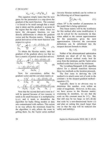
C ŢICLEANU
2
amin
acur
c
(6)
a
cur
This equation simply states that the next
guess for the parameters is a step down the
gradient of the merit function. The constant
c is forced to be small enough that a small
step is taken and the gradient is accurate in
the region that the step is taken. Since we
know the chi-square function, we can
directly differentiate to obtain the gradient
vector and the Hessian matrix. Taking the
partial derivatives of the merit function with
respect to a gives
To obtain the Hessian matrix, take the
gradient of the gradient above (so that we
have a matrix of partial second derivatives):
2 2
N
1 yxi
; a
yxi
; a
2
2
ak
al
i1
i ak
al
(8)
2
y i y xi
; a y xi
; a
2
a
a
i
l
Now, for convenience, define the
gradient vector and the curvature matrix as
2
1
N yi
yxi
; a
yxi
; a
Gk
(9)
2
2 ak
i1 i
ak
2 2
N 1 yx
i ; a y xi
; a
Ckl
(10)
2
akal
i1 i
ak
al
Note that the second derivative term in C
will be ignored because of two reasons: it
tends to be small because it is multiplied by
(y-yi), and it tends to destabilize the
algorithm for badly fitting models or data
sets contaminated with outliers. This action
in no way affects the minimum found by
the algorithm; it only affects the route in
getting there. So, the Taylor series method
k
(inverse Hessian method) can be written as
the following set of linear equations:
50 Ingineria Iluminatului 2010; 12, 2: 45-54
NP
C a
G
k 1
kl
l
k
(11)
where NP is the number of parameters in
the model that is being optimized.
This linear matrix will be the workhorse
for this method after some modification; it
can be solved for the increments a that,
when added to the current approximation
for the parameters, gives the next
approximation. Likewise, the convenient
definitions can be substituted into the
steepest descent formula to obtain
a cG
(12)
l
Neither of the aforementioned optimization
methods are ideal all of the time; the
steepest descent method works best far
away from the minimum, and the Taylor series
method works best close to the minimum.
The Levenberg-Marquardt (LM) algorithm
allows for a smooth transition between
these two methods as the iteration proceeds.
The first issue in deriving the LM
method is to attach some sort of scale to the
constant c in the steepest-gradient method -
equation (12).
Typically, there is no obvious way to
determine this number, even within an
order of magnitude. However, in this case,
we have access to the Hessian matrix;
examining its members, we see that the
scale on this constant must be 1/Cll. But,
that still may be too large, so let's divide
that scale by a non-dimensional factor ()
and plan on setting this much larger than
one so that the step will be reduced (for
safety and stability).
l