Refresh - Inpe
Refresh - Inpe
Refresh - Inpe

You also want an ePaper? Increase the reach of your titles
YUMPU automatically turns print PDFs into web optimized ePapers that Google loves.
Preliminary results of simulations of a user-friendly fast line-by-line computer code<br />
for simulations of satellite signal<br />
Marcelo de Paula Corrêa<br />
Rodrigo Augusto Ferreira de Souza<br />
Juan Carlos Ceballos<br />
Boris Fomin<br />
Divisão de Satélites e Sistemas Ambientais<br />
Centro de Previsão de Tempo e Estudos Climáticos<br />
Instituto Nacional de Pesquisas Espaciais<br />
Rod. Pres. Dutra, km 40 – Cachoeira Paulista – SP – CEP 12630-000<br />
{mpcorrea, rodrigo, ceballos, fomin}@cptec.inpe.br<br />
Resumo. Este trabalho descreve resultados de um código computacional linha-a-linha rápido (FLISS – Fast<br />
LIne-by-line Satellite signal Simulator), desenvolvido no CPTEC/INPE para fins de análise de impacto de<br />
diferentes perfis atmosféricos no sinal detectado por sensores de satélites. A informação line-by-line baseada na<br />
base de dados HITRAN permite adaptar o cálculo para funções-resposta arbitrárias para diferentes detectores.<br />
Apresenta-se a versão do código para o espectro de radiação térmica infravermelha (FLISS-L) em comparações<br />
com as temperaturas de brilho obtidas pelos sensores AIRS do Aqua (mais de 2000 canais), MODIS, AVHRR e<br />
HIRS do satélite NOAA 16, e Imager do GOES-12. Foi escolhida uma região oceânica com céu claro. Embora<br />
um caso real apresente limitações com relação à definição exata de perfis de temperatura e concentrações de<br />
gases, os resultados mostram boa concordância com as observações. Isto é observado em particular para<br />
detectores com faixa espectral mais larga, encontrando-se diferenças inferiores a 2K. O utilitário foi desenhado<br />
para ter comportamento acessível (user-friendly), de forma que novos perfis de atmosfera e características novas<br />
de um sensor possam ser introduzidos facilmente.<br />
Abstract. This paper describes results of a fast line-line-by-line computer code (FLISS – Fast LIne-by-line<br />
Satellite signal Simulator), which was developed at CPTEC/INPE for analyzing the impact of different<br />
atmospheric profiles on spectral signal detected by satellite sensors. Line-by-line information based on HITRAN<br />
database allows calculations adapted to any spectral response function of a detector. It is presented a comparison<br />
of the code, infrared FLISS-L version, with brightness temperatures obtained by Aqua AIRS sensor (more than<br />
2000 channels), as well as Aqua MODIS, NOAA AVHRR and HIRS, and GOES-12 Imager. An oceanic cloudfree<br />
region was chosen. Although a real case presents some limitations concerning exact definition of profiles<br />
for atmospheric temperature and gas concentration, the results show fairly good agreement with observations.<br />
This is particularly true for spectrally wider detectors, showing differences lower than 2 K. The software was<br />
designed for user-friendly behavior, such that atmospheric profiles and new detector characteristics can be easily<br />
introduced.<br />
Palavras-chave: modelo linha-a-linha, FLISS, satélite, sensoriamento remoto, infravermelho AIRS, MODIS,<br />
AVHRR, GOES, HIRS.<br />
Keywords: line-by-line code, FLISS, satellites, remote sensing, infrared, AIRS, MODIS, AVHRR, GOES,<br />
HIRS.<br />
363
1. Introduction<br />
There exist a number of softwares for radiative transfer calculations, including those that perform<br />
satellite signal simulation. Examples of well-known codes are: LOWTRAN (Kneysis et al., 1988),<br />
SBDART (Ricchiazzi et al., 1998), 5S (Tanré et al., 1986) and its new 6S version (Vermote et al.,<br />
1997). Historically, one of the main concerns refers to an efficient match between required accuracy<br />
and available processing time. In the lack of such matching, precise radiative codes tend to be used<br />
only for benchmark calculations, sensibility tests and hypotheses validations. Fast calculations are<br />
mainly performed on the base of narrowband parameterizations. Nevertheless, recent personal<br />
computers have attained a performance thinking of powerful mainframes a decade ago.<br />
This fact suggests the convenience of developing fast radiative transfer codes based on line-byline<br />
information, which could provide the highest accuracy presently available with reasonably low<br />
computation cost. The proposed challenge implies in developing proper methods for working with<br />
HITRAN database, whose version 2004 includes 1,734,469 spectral lines for 37 different molecular<br />
species (http://www.hitran.com). Such radiative code should allow inclusion of proper information<br />
about atmospheric structure and satellite sensor spectral response, providing tools to discuss accuracy<br />
of sensor quality and design of new sensors, as well as to improve understanding of the influence of<br />
atmospheric gases (natural and anthropogenic) and parameterize their effects.<br />
A new radiative code was developed at the Divisão de Satélites e Sistemas Ambientais<br />
(DSA/CPTEC/INPE), which seeks to answer to the abovementioned requirements. It is labeled as<br />
FLISS (Fast Line-by-line Satellite signal Simulator). The present work shows preliminary results of<br />
using FLISS-L version for simulated brightness temperature in the longwave (infrared) interval,<br />
expected for several satellite sensors. It has been considered a real case of atmospheric profile over<br />
Atlantic Ocean. Comparison with measurements performed by the actual sensors is presented and<br />
discussed.<br />
2. Algorithm Description<br />
The latest version of spectral database HITRAN-11 v (Rothman et al., 2003) and continuum<br />
model by N2, O2, O3, CO2 and H2O (CKD-2.4) have been used in FLISS, based on the same physical<br />
assumptions used in the carefully validated Line-by-Line Radiation Transfer Model (LBLRTM)<br />
(Clough et al., 1992; Clough and Iacono, 1995). However, FLISS makes use of other line-by-line<br />
algorithms for gas absorption calculations (Fomin, 1994) and vertical integration (Fomin et al., 2004).<br />
The use of this line-by-line method not only increases the accuracy but also performs different<br />
applications in any spectral width interval, avoiding previous development of gas absorption<br />
parameterizations. The FLISS main feature is the clear physical meaning of calculation procedures.<br />
For instance, spectral resolution in FLISS is varied automatically so that the narrowest spectral line<br />
can be adequately sampled.<br />
The new feature introduced by FLISS is the user-friendly interface for input of several<br />
information and a computational speed being higher than those of usual LBL codes found in the<br />
literature. Present FLISS version provides several default data bases for the user: a) model<br />
atmospheric profiles (McClatchey et al., 1972); b) spectral ground reflectances; c) response function<br />
for several sensors (MODIS, AIRS, AVHRR, HIRS and GOES Imager). Also, the user can introduce<br />
your own version of these data. FLISS is a multi-platform computer program developed in Fortran90,<br />
compatible with MS-Windows, Linux and UNIX. Presently, it has two versions for specific spectral<br />
regions: FLISS-S for solar radiation, including applications for clouds and aerosols, and FLISS-L for<br />
infrared and microwave spectrum. Version L does not include absorption/scattering by atmospheric<br />
particulate (aerosol or cloud).<br />
364
3. Methods and Data<br />
Brightness temperature data collected by DSA/CPTEC/INPE were considered (sensors AVHRR<br />
and HIRS in NOAA-16; AIRS and MODIS in Aqua; GOES-12 Imager), selected through clear-sky<br />
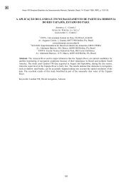
pixels in images over Atlantic Ocean. Based on these needs, we chose 30 th August 2004 for the<br />
comparisons. Figure 1 illustrates geographical position of the selected point (26°S, 43°W), for which<br />
pixels of the various sensors were chosen. For FLISS-L calculations, retrieved and theoretical profiles<br />
were introduced. It was used NASA retrievals (provided by Aqua satellite) of air and surface<br />
temperatures and moisture and O3 profiles. For other gases (CO2, CH4, N2O, O2) a midlatitude summer<br />
model profile (McClatchey et al., 1972) was adopted.<br />
Figure 1 – Quick look of the region of study (visible AIRS channels)<br />
AIRS sensor has 2378 channels in infrared spectrum, while the other sensors include a number of<br />
channels not exceeding a couple of dozens. Table 1 illustrates spectral positions of last ones. Figure 2<br />
(observed and simulated results) allows seeing the spectral distribution of these sensors.<br />
Sensor Channel number (spectral interval in µm)<br />
20 (3.66 – 3.84); 21 (3.93 – 3.99); 22 (3.93 – 3.99); 23 (4.02 – 4.08);<br />
24 (4.43 – 4.50); 25 (4.48 – 4.55); 27 (6.54 – 6.90); 28 (7.18 – 7.48);<br />
MODIS<br />
29 (8.40 – 8.70); 30 (9.58 – 9.88); 31 (10.78 – 11.28); 32 (11.77 – 12.27);<br />
33 (13.19 – 13.49); 34 (13.49 – 13.79); 35 (13.79 – 14.09); 36 (14.09 – 14.39)<br />
GOES-12 Imager 2 (3.78 – 4.03); 3 (6.47 – 7.02); 4 (10.2 – 11.2); 5 (11.5 –12.5)<br />
1 (14.88 – 15.02); 2 (14.49 – 14.93); 3 (14.25 – 14.75); 4 (13.91 – 14.56);<br />
5 (13.66 – 14.29); 6 (13.35 – 13.95); 7 (13.07 – 13.64); 8 (10.70 – 11.56);<br />
HIRS<br />
9 (9.48 – 9.95); 10 (12.22 – 12.72); 11 (7.12 – 7.55); 12 (6.20 – 6.88);<br />
13 (4.52 – 4.62); 14 (4.48 – 4.57); 15 (4.43 – 4.52); 16 (4.41 – 4.50);<br />
17 (4.09 – 4.17); 18 (3.93 – 4.02); 19 (3.62 – 3.91)<br />
AVHRR 3 (3.55 – 3.93); 4 (10.3 – 11.3); 5 (11.5 – 12.5)<br />
Table 1 – Spectral intervals of the satellite sensors<br />
365
4. Results<br />
Figure 2 – Brightness temperature for different sensors: observations and calculations.<br />
Figure 2 allows a general comparison of observed and simulated brightness temperatures and<br />
figures 3 (a,b,c,d) provide more detailed observations for discussion of results.<br />
Figure 3a presents the spectral interval between 3.6 and 4.8 µm, characterized by an atmospheric<br />
window and neighboring absorption/emission bands for water vapor (H2O), carbon dioxide (CO2) and<br />
nitrous oxide (N2O). Differences lower than 2 K are evident within the atmospheric window. It is<br />
worthwhile to note that AVHRR, MODIS and GOES channels in this spectral region are used for fire<br />
detection. Differences become high for λ > 4 µm, especially where influence of N2O is expected (this<br />
gas has variable concentration in the atmosphere).<br />
Figure 3b (6.0 to 8.0 µm) exhibits strong absorption/emission by H2O by a CH4 band. The<br />
comparison makes evident limitations for narrowband channels simulation in this complex region,<br />
while wider spectral channels of other sensor show fairly good agreement.<br />
Figure 3c illustrates results for the mid-infrared atmospheric window and the 9.6 µm ozone band.<br />
Agreement between simulated and observed temperatures is good throughout the window (differences<br />
lower than 1.5 K), except for GOES channel 4. One simple reason for these small differences may be<br />
attributed to electronic noise. For 9.6 µm region, systematic differences of about 5 K are observed.<br />
This behavior could be due to a somewhat poor ozone and/or temperature profile by the NASA Aqua<br />
retrieval procedure within the stratosphere, where ozone absorption/emission is more intense.<br />
Figure 3d shows the 14 µm CO2 absorption band region, usually used for temperature retrieval of<br />
the atmosphere. Here, difference between simulation and observation is systematically positive for<br />
wideband detectors, between +2 K and +6.6 K; nevertheless, they are still better than results for the<br />
narrower AIRS channels. For this sensor, discrepancies are not random and show oscillations between<br />
+5 K and –15 K along this spectral region. Several reasons can be drawn for this behavior; among<br />
others, it may be due to influence of water vapor continuum, adopted CO2 profile (constant<br />
concentration of 370 ppm), or even deviations between retrieved and actual temperature profile.<br />
366
Figure 3a – Atmospheric window (3.6 µm), water vapor, nitrous oxide and carbon dioxide bands.<br />
Figure 3b – Water vapor, carbon dioxide, nitrous oxide and methane bands.<br />
367
Figure 3c – Atmospheric window with ozone absorption band (9.6 µm).<br />
Figure 3d – Water vapor and carbon dioxide bands.<br />
368
5. Conclusions and Perspectives<br />
Only one test of FLISS-L performance has been presented. However, it strongly suggests a<br />
generally good agreement between simulation and real data for five different satellite sensors in<br />
infrared thermal spectrum. In the case of AIRS sensor, with more than 2000 spectrally narrow<br />
channels, the general average of differences was +1.8 K with standard deviation 4.2 K. These values<br />
are lower for the atmospheric window (+1.5 ± 1.1 K), they amount +2.9 ± 2.7 K in the ozone band<br />
region and +5.3 ± 1.9 K in the 6.4 µm in the strong water vapor band. Improvements in results could<br />
be obtained by: a) better definition of temperature and gaseous concentration profiles (radiosonde<br />
profiles would be recommended); b) updated definition of response functions (in particular, those of<br />
AIRS sensor); c) careful choice of cloud-free pixels; d) precise estimation of ground reflectance and<br />
temperature (ocean surface was considered in this paper, certainly suitable for this type of comparison;<br />
tests over land surface should be exhibit larger differences). It must be stressed that spectrally narrow<br />
channel signal is a delicate matter of estimation; in this context, spectral behavior of some<br />
atmospheric gases (in particular water vapor) is not necessarily well defined and is still a matter of<br />
research by the world main groups of spectroscopy (see http://www.hitran.com). Last but not least,<br />
atmospheric composition considered in this paper does not include all available gas data. HITRAN<br />
includes 37 species. In the case of spectrally wider sensors, similar recommendations are appropriate;<br />
nevertheless, it seems evident that a wider spectral interval tends to lower (or compensate) the effects<br />
of unknowing the spectrally most fine structure of atmospheric radiation.<br />
The results suggest that the software may attain fairly good estimates with spectral high<br />
definition, being appropriate for simulation of behavior of the new generation of environmental<br />
satellites. It is worthwhile to note that FLISS-L does not depend on previous parameterizations of<br />
radiative transmittance but strictly on line-by-line calculations. Present version has a user-friendly<br />
interface, which permits its use for other sensors and cloud-free atmospheric profiles. FLISS-L can be<br />
used not only for simulation of sensor signals, but also for parameterizing gas content and its<br />
fluctuations as a function of observed signal. The tests presented in this paper were run in a personal<br />
computer Pentium 4, with 2.80 GHz clock , 512 MB RAM and MS-Windows operational system.<br />
Acknowledgments<br />
This work has partially supported by the CNPq foundation (grant 301263019), Brazil.<br />
References<br />
Clough, S. A.; Iacono M. J.; Moncet J.-L. Line-by-line calculation of atmospheric fluxes and cooling rates:<br />
Application to water vapor. Journal of Geophysical Research, v. 97, p. 15761-15785, 1992.<br />
Clough, S.A.; Iacono, M.J. Line-by-line calculations of atmospheric fluxes and cooling rates II: Application to<br />
carbon dioxide, ozone, methane, nitrous oxide, and the halocarbons. Journal of Geophysical Research, v. 100 ,<br />
n. 16, p. 519-16,535, 1995.<br />
Fomin, B.A. Benchmark computation for solar fluxes and influxes in aerosol and cloudy atmosphere. Izvetyia<br />
Atmospheric Oceanic Physics, v. 30, n. 3, p. 283-290, 1994.<br />
Fomin, B.A. A Distribution Technique for Radiative Transfer Simulation in Inhomogeneous Atmosphere: 1.<br />
FKDM, Fast K-Distribution Model for the Longwave, Journal of Geophysical Research-Atmospheres, v. 109,<br />
n. D2, D02110, paper n. 10.1029/2003JD003802, 2004.<br />
Kneizys, F.X.; Shettle, E.P.; Abreu, L.W.; Chetwynd, J.H.; Anderson, G.P.; Gallery, W.O.; Selby; J.E.A.;<br />
Clough, S.A.. Users guide to LOWTRAN-7. Environmental Research Papers, n. 1010, Publ. AFGL-TR-88-<br />
0177, Air Force Geophys. Lab., Hanscom, 146 p., 1988.<br />
Mc Clatchey, R.A.; Fenn, R.W.; Selby, J.E.A.; Volz, F.E.; Garing, J.S. Optical properties of the atmosphere.<br />
Publ. AFCRL-72-0497, Air Force Cambridge Res. Lab., Hanscom, 1972.<br />
Ricchazzi, P.; Yang, S. R. SBDART: A research and teaching software tool for Plane-parallel radiative transfer<br />
in the earth's atmosphere. Bulletin of the American Meteorological Society, v. 79, n. 10, p. 2101-2114, 1998.<br />
369
Tanre, D.; Deroo, C., Duhaut, P., Herman, M., Morcrette, J. J.; Perbos, J.; Deschamps, P.Y. Simulation of the<br />
satellite signal in the solar spectrum (5S). Technical Report of Laboratorire d'Optique Atmospherique<br />
Université des Sciences et Techniques de Lille, 149pp, 1986.<br />
Rothman, L.S. et al. The HITRAN molecular spectroscopic database: edition of 2000 including updates through<br />
2001. Journal of Quantitative Spectroscopy and Radiative Transfer, v. 82, p. 5-44, 2003.<br />
Vermote, E. F.; Tanré, D.; Deuzé, J. L.; Herman, M.; Morcette, J. J. Second Simulation of the Satellite Signal in<br />
the Solar Spectrum, 6S: An Overview. IEEE Transactions on Geoscience and Remote Sensing, v. 35, p. 675-<br />
686, 1997.<br />
370