Download Sample pages 1 (pdf, 5.5 MB) - Springer

More documents

Recommendations

Info

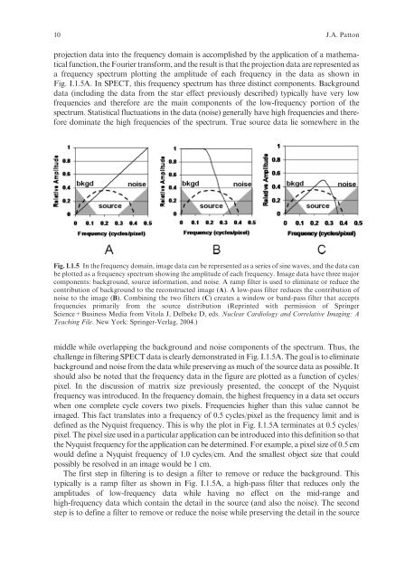
10 J.A. Patton projection data into the frequency domain is accomplished by the application of a mathematical function, the Fourier transform, and the result is that the projection data are represented as a frequency spectrum plotting the amplitude of each frequency in the data as shown in Fig. I.1.5A. In SPECT, this frequency spectrum has three distinct components. Background data (including the data from the star effect previously described) typically have very low frequencies and therefore are the main components of the low-frequency portion of the spectrum. Statistical fluctuations in the data (noise) generally have high frequencies and therefore dominate the high frequencies of the spectrum. True source data lie somewhere in the Fig. I.1.5 In the frequency domain, image data can be represented as a series of sine waves, and the data can be plotted as a frequency spectrum showing the amplitude of each frequency. Image data have three major components: background, source information, and noise. A ramp filter is used to eliminate or reduce the contribution of background to the reconstructed image (A). A low-pass filter reduces the contribution of noise to the image (B). Combining the two filters (C) creates a window or band-pass filter that accepts frequencies primarily from the source distribution (Reprinted with permission of <strong>Springer</strong> Science+Business Media from Vitola J, Delbeke D, eds. Nuclear Cardiology and Correlative Imaging: A Teaching File. New York: <strong>Springer</strong>-Verlag, 2004.) middle while overlapping the background and noise components of the spectrum. Thus, the challenge in filtering SPECT data is clearly demonstrated in Fig. I.1.5A. The goal is to eliminate background and noise from the data while preserving as much of the source data as possible. It should also be noted that the frequency data in the figure are plotted as a function of cycles/ pixel. In the discussion of matrix size previously presented, the concept of the Nyquist frequency was introduced. In the frequency domain, the highest frequency in a data set occurs when one complete cycle covers two pixels. Frequencies higher than this value cannot be imaged.Thisfacttranslatesinto a frequency of 0.5 cycles/pixel as the frequency limit and is defined as the Nyquist frequency. This is why the plot in Fig. I.1.5A terminates at 0.5 cycles/ pixel. The pixel size used in a particular application can be introduced into this definition so that the Nyquist frequency for the application can be determined. For example, a pixel size of 0.5 cm would define a Nyquist frequency of 1.0 cycles/cm. And the smallest object size that could possibly be resolved in an image would be 1 cm. The first step in filtering is to design a filter to remove or reduce the background. This typically is a ramp filter as shown in Fig. I.1.5A, a high-pass filter that reduces only the amplitudes of low-frequency data while having no effect on the mid-range and high-frequency data which contain the detail in the source (and also the noise). The second step is to define a filter to remove or reduce the noise while preserving the detail in the source
I.1 History and Principles of Hybrid Imaging 11 data. This is accomplished using a low-pass filter as shown in Fig. I.1.5B, which accepts selected frequencies up to a certain value. There are a number of low-pass filters that are available for processing SPECT data. Some have fixed characteristics, and others have flexibility in choosing the cutoff frequency and/or the slope of the filter. Some filters are optimized for image data with excellent counting statistics, and others provide the capability for filtering data with poor statistics. Also, the amount of detail in an image and the object sizes to be resolved (spatial resolution) are important factors to be considered in the selection of a filter. In practice, the lowpass filter may be applied first to reduce the effects of noise, and then the ramp filter is applied to reduce background. The two filters may be combined as shown in Fig. I.1.5C to function as a band-pass filter. It can be seen in the latter figure that appropriate selection of the cutoff frequency will eliminate much of the noise, and selecting an appropriate filter shape will preserve most of the source data. The terms under-filtering and over-filtering were previously referenced, and examples were shown in Fig. I.1.4. From Fig. I.1.5C, it can be observed that, when a cutoff frequency is chosen that is too low, someofthesourcedatawillbeexcludedfrom the final image, and this situation is referred to as over-filtering. Similarly, when too high a cutoff frequency is chosen, excessive noise will be included in the final image, and this is referred to as under-filtering. In clinical applications, most imaging systems provide the capability for trying different filters and filter parameters on a single slice of image data in order to select the appropriate processing algorithm for a specific patient study. Technologists and physicians in the clinical setting often prefer this method of trial and error. Iterative Reconstruction Filtered backprojection amplifies statistical noise, which adversely affects image quality. To address this problem, Shepp and Vardi introduced an iterative reconstruction technique in 1982 10 based on the theory of expectation maximization (EM), which has a proven theoretical convergence to an estimate of the actual image distribution that has a maximum likelihood of having projections most similar to the acquired projections. The initial implementation of these algorithms was very time consuming, with several iterations being required to reach a solution, and extensive computer power was required. Since that time, much effort has been expended in improving and testing algorithms based on this concept. Significant improvements in speed and signal-to-noise and reconstruction accuracy have resulted from these efforts. In 1994, Hudson and Larkin 11 developed the technique of ordered sets EM (OS-EM) for image reconstruction from 2D projection data. This algorithm was based on the concept of dividing the projection data into small subsets (e.g., paired opposite projections in SPECT data) and performing the EM algorithm on each subset. The solution of each subset was used as the starting point for the next subset, with subsequent subsets being selected to provide the maximum information (e.g., chose the second subset of data to be orthogonal to the first subset). The advantage of this technique is that, at the end of the first pass, the entire data set has been processed one time, but n successive approximations to the final solution have been made where n is the number of subsets. Thus, OS-EM is n times faster than the original EM algorithm. Typically, only two to three passes through the data set (iterations) are required for the reconstructed image to converge to a final value that is essentially unchanged by further iterations. Correction for scatter and attenuation effects (topics that will be discussed later) can be performed on the acquired projection data during the reconstruction process. The advantage of this technique is that the star effect inherent in filtered backprojection is virtually eliminated since the acquired data are distributed within the body contour. Because of this
Page 1 and 2: Chapter I.1 History and Principles
Page 3 and 4: I.1 History and Principles of Hybri
Page 7: I.1 History and Principles of Hybri

Download Sample pages 1 (pdf, 5.5 MB) - Springer

Create successful ePaper yourself

Delete template?

Save as template?