View Carlson-Titman-Tiu Paper - The Paul Merage School of Business

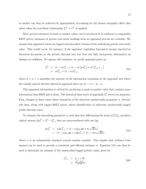
to market can then be achieved by appropriately accounting for the Jensen inequality effect that
arises when the non-linear relationship V P
t = e vP t is applied.
More precise estimates of mark to market values can be produced if, in addition to comparable
REIT prices, estimates of private real estate holdings from an appraisal process are available. We
assume that appraised values are lagged and smoothed versions of the underlying private real estate
value. This would occur, for instance, if the appraiser capitalizes forecasted income reported in
historical documents at the private discount rate but does not fully incorporate information on
changes in cashflows. To capture this intuition, we model appraisal prices as
ˆv P t = (1 − α)vP t−1 + (1 − α) αvP t−2 + α2vP t−3 + ...
= αˆv P t−1 + (1 − α)vP t−1 ,
where 0 ≤ α < 1 quantifies the amount of old information remaining in the appraisal and where
the equally spaced discrete historical appraisal dates are {t − 1, t − 2, ...}.
This appraisal information is critical for producing a mark-to-market value that contains more
information than REIT prices alone. The historical time series of appraisals ˆv P t serves two purposes.
First, changes in these values allow estimation of the otherwise unobservable parameter α. Second,
this data, along with lagged REIT prices, allows identification of otherwise unobservable lagged
public discount rates.
To estimate the smoothing parameter α, note that first differencing the series {ˆv P t } ∞ t=1 produces
capital returns ∆v P t = ˆv P t − ˆv P t−1
that are autocorrelated with one lag
∆vP t = α∆vP t−1 + (1 − α)[µL∆t
√
+ σL ∆tɛt]
= (1 − α)µL∆t + α∆v P t−1
√
+ (1 − α)σL ∆tɛt
where ɛt is an independent standard normal random variable. This implies that ordinary least
squares can be used to provide a consistent and efficient estimate ˆα. Equation (18) can then be
used to determine an estimate of the unsmoothed lagged private value, given by
v P t−1 = lt−1 + Φ
= ˆvP t −ˆαˆvP t−1
1−ˆα .
13
(18)
(19)
(20)