View Carlson-Titman-Tiu Paper - The Paul Merage School of Business

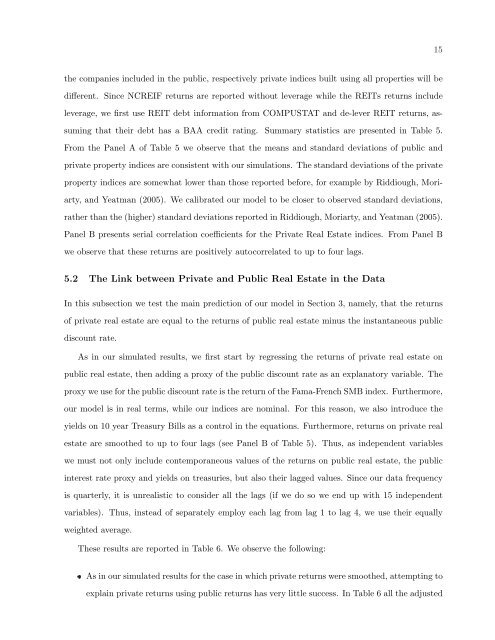
the companies included in the public, respectively private indices built using all properties will be
different. Since NCREIF returns are reported without leverage while the REITs returns include
leverage, we first use REIT debt information from COMPUSTAT and de-lever REIT returns, as-
suming that their debt has a BAA credit rating. Summary statistics are presented in Table 5.
From the Panel A of Table 5 we observe that the means and standard deviations of public and
private property indices are consistent with our simulations. The standard deviations of the private
property indices are somewhat lower than those reported before, for example by Riddiough, Mori-
arty, and Yeatman (2005). We calibrated our model to be closer to observed standard deviations,
rather than the (higher) standard deviations reported in Riddiough, Moriarty, and Yeatman (2005).
Panel B presents serial correlation coefficients for the Private Real Estate indices. From Panel B
we observe that these returns are positively autocorrelated to up to four lags.
5.2 The Link between Private and Public Real Estate in the Data
In this subsection we test the main prediction of our model in Section 3, namely, that the returns
of private real estate are equal to the returns of public real estate minus the instantaneous public
discount rate.
As in our simulated results, we first start by regressing the returns of private real estate on
public real estate, then adding a proxy of the public discount rate as an explanatory variable. The
proxy we use for the public discount rate is the return of the Fama-French SMB index. Furthermore,
our model is in real terms, while our indices are nominal. For this reason, we also introduce the
yields on 10 year Treasury Bills as a control in the equations. Furthermore, returns on private real
estate are smoothed to up to four lags (see Panel B of Table 5). Thus, as independent variables
we must not only include contemporaneous values of the returns on public real estate, the public
interest rate proxy and yields on treasuries, but also their lagged values. Since our data frequency
is quarterly, it is unrealistic to consider all the lags (if we do so we end up with 15 independent
variables). Thus, instead of separately employ each lag from lag 1 to lag 4, we use their equally
weighted average.
These results are reported in Table 6. We observe the following:
As in our simulated results for the case in which private returns were smoothed, attempting to
explain private returns using public returns has very little success. In Table 6 all the adjusted
15