Lab Report on the Fabry-Perot-Etalon - of Michael Goerz
Lab Report on the Fabry-Perot-Etalon - of Michael Goerz
Lab Report on the Fabry-Perot-Etalon - of Michael Goerz

You also want an ePaper? Increase the reach of your titles
YUMPU automatically turns print PDFs into web optimized ePapers that Google loves.
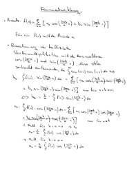
<str<strong>on</strong>g>Lab</str<strong>on</strong>g> <str<strong>on</strong>g>Report</str<strong>on</strong>g> <strong>on</strong> <strong>the</strong> <strong>Fabry</strong>-<strong>Perot</strong>-Etal<strong>on</strong><br />
GP II<br />
Tutor: M. Fushitani<br />
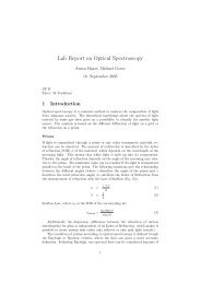
1 Introducti<strong>on</strong><br />
Multi-Ray-Interference<br />
Ant<strong>on</strong> Haase, <strong>Michael</strong> <strong>Goerz</strong><br />
4. October 2005<br />
The diffracti<strong>on</strong> pattern <strong>of</strong> a single and double slit is a well-known interference<br />
phenomen<strong>on</strong>, where <strong>the</strong> double slit produces more fringes than <strong>the</strong> single slit.<br />
By increasing <strong>the</strong> number <strong>of</strong> slits (using a grid instead, for example), we get<br />
a sharper pattern with small areas <strong>of</strong> c<strong>on</strong>structive interference and large areas<br />
<strong>of</strong> destructive interference. This is <strong>the</strong> result <strong>of</strong> multi-ray-interference behind a<br />
regular structure <strong>of</strong> defracting elements. Huygens Principle is a simple geometric<br />
explanati<strong>on</strong> for <strong>the</strong> observati<strong>on</strong> behind such a setup. The higher number <strong>of</strong> slits<br />
leads to a multiplicati<strong>on</strong> <strong>of</strong> <strong>the</strong> wavelength difference, so that <strong>the</strong> c<strong>on</strong>diti<strong>on</strong> for<br />
destructive interference is reached at a lower angle difference (from <strong>the</strong> angle <strong>of</strong><br />
<strong>the</strong> related maximum) than behind a single slit. This means that <strong>the</strong> maxima<br />
are sharper and <strong>the</strong> resoluti<strong>on</strong> in a spectral applicati<strong>on</strong> is higher.<br />
<strong>Fabry</strong>-<strong>Perot</strong>-Etal<strong>on</strong><br />
The <strong>Fabry</strong>-<strong>Perot</strong>-Etal<strong>on</strong> (FBE) is a optical res<strong>on</strong>ator and a realizati<strong>on</strong> <strong>of</strong> a multiray-interference<br />
device. It c<strong>on</strong>sists <strong>of</strong> two parallel, semipermeable mirrors with<br />
an optical medium in between. Incoming light <strong>of</strong> a certain angle is partially<br />
transmitted and reflected between <strong>the</strong> two surfaces as shown in Fig. 1. The<br />
resulting phase difference between two rays can be calculated with a simple<br />
geometric interpretati<strong>on</strong> (vector additi<strong>on</strong>).<br />
δ = AC + CD − AB = 2 d cos(α) (1)<br />
The phase difference <strong>of</strong> two rays must be δ = nλ to get c<strong>on</strong>structive interference.<br />
The values <strong>of</strong> n are called <strong>the</strong> order <strong>of</strong> interference.<br />
The <strong>Fabry</strong>-<strong>Perot</strong>-Etal<strong>on</strong> realizes a very high amount <strong>of</strong> interacting rays and<br />
interference orders. Therefore it is a highly accurate device, used to distinguish<br />
small wavelength differences in spectroscopy, for example (high resoluti<strong>on</strong>).<br />
Dispersi<strong>on</strong> Range<br />
The spectral range <strong>of</strong> light which can be analyzed by an optical device like <strong>the</strong><br />
<strong>Fabry</strong>-<strong>Perot</strong>-Etal<strong>on</strong> is limited. The difference between two bordering lines can<br />
1
GP2 - FAP Haase, <strong>Goerz</strong><br />
Fig. 1: <strong>Fabry</strong>-<strong>Perot</strong>-Etal<strong>on</strong><br />
be <strong>the</strong> value <strong>of</strong> <strong>the</strong> interference order or a small wavelength difference. The<br />
interference c<strong>on</strong>diti<strong>on</strong> for this case is:<br />
From this follows <strong>the</strong> dispersi<strong>on</strong> range.<br />
(z + 1)λ = z(λ + ∆λ) (2)<br />
∆λ = λ<br />
z<br />
The high interference order <strong>of</strong> <strong>the</strong> FPE menti<strong>on</strong>ed in <strong>the</strong> beginning, and <strong>the</strong><br />
resulting low dispersi<strong>on</strong> range, makes it a perfect device to analyze nearly<br />
m<strong>on</strong>ochromatic light.<br />
<strong>Fabry</strong>-<strong>Perot</strong>-Spectrometer<br />
The advantages <strong>of</strong> <strong>the</strong> FBE as a spectrometer have already been explained.<br />
The spectrometer is realized with incoming divergent light and a lens to project<br />
<strong>the</strong> interference pattern <strong>on</strong> an observati<strong>on</strong> plane. The image <strong>the</strong>n c<strong>on</strong>sists <strong>of</strong><br />
c<strong>on</strong>centric circles. The interfence c<strong>on</strong>diti<strong>on</strong> for this specific setup is<br />
z = 2d<br />
λ<br />
(3)<br />
<br />
1 − r2<br />
2f 2<br />
<br />
, (4)<br />
where f is <strong>the</strong> focal length <strong>of</strong> <strong>the</strong> lens, r is <strong>the</strong> radius <strong>of</strong> <strong>the</strong> observed circle and<br />
α was set to α = r<br />
1<br />
f and cos(α) = 1 − 2α2 , respectively.<br />
The measurement <strong>of</strong> at least two circles would be enough to calculate <strong>the</strong><br />
distance between <strong>the</strong> two mirrors <strong>of</strong> <strong>the</strong> etal<strong>on</strong>. The equati<strong>on</strong> comes from c<strong>on</strong>diti<strong>on</strong><br />
(4) by combining it for <strong>the</strong> two values <strong>of</strong> r to<br />
d = i<br />
λf 2<br />
r 2 i + r2 0<br />
, (5)<br />
where i is <strong>the</strong> number <strong>of</strong> circles counted from <strong>the</strong> innermost circle (i = 0).<br />
Additi<strong>on</strong>ally, we get <strong>the</strong> relative weavelength difference by measuring <strong>the</strong><br />
radius <strong>of</strong> a certain order for two separate wavelengths:<br />
∆λ ≈ λ<br />
2f 2<br />
2 ′2<br />
r − r <br />
The accuracy <strong>of</strong> this calculati<strong>on</strong> is determined by <strong>the</strong> accuracy <strong>of</strong> <strong>the</strong> radius<br />
measurement. To use <strong>the</strong> high efficiency <strong>of</strong> <strong>the</strong> FBE, it is necessary to calibrate<br />
<strong>the</strong> device. This can be d<strong>on</strong>e with light <strong>of</strong> a well known wavelength. The<br />
wavelength <strong>the</strong>n will be calculated directly from <strong>the</strong> interference c<strong>on</strong>diti<strong>on</strong>.<br />
2<br />
(6)
GP2 - FAP Haase, <strong>Goerz</strong><br />
Resoluti<strong>on</strong> <strong>of</strong> <strong>the</strong> <strong>Fabry</strong>-<strong>Perot</strong>-Spectrometer<br />
The resoluti<strong>on</strong> <strong>of</strong> <strong>the</strong> FPS can be calculated with <strong>the</strong> Equati<strong>on</strong> <strong>of</strong> Airy. It<br />
depends <strong>on</strong> <strong>the</strong> transmissi<strong>on</strong> and reflecti<strong>on</strong> coefficient <strong>of</strong> <strong>the</strong> mirrors.<br />
I<br />
I0<br />
=<br />
<br />
T<br />
1 − R<br />
2 1<br />
1 + 4R<br />
(1+R) 2 sin 2 (φπ)<br />
From this we get <strong>the</strong> full width at half maximum.<br />
2 Assignments<br />
1. C<strong>on</strong>struct and adjust <strong>the</strong> setup.<br />
1 − R<br />
2∆z =<br />
π √ R<br />
2. Calculate <strong>the</strong> distance between <strong>the</strong> two planes <strong>of</strong> <strong>the</strong> FBE using <strong>the</strong> red<br />
line (643.9 nm) <strong>of</strong> an cadmium lamp and determine <strong>the</strong> interference order.<br />
3. Calculate <strong>the</strong> wavelength <strong>of</strong> <strong>the</strong> green and darkblue line <strong>of</strong> <strong>the</strong> cadmium<br />
lamp.<br />
4. Give an approximate value for <strong>the</strong> width <strong>of</strong> <strong>the</strong> maxima lines <strong>of</strong> <strong>the</strong> red<br />
line and compare <strong>the</strong>m to <strong>the</strong> <strong>the</strong>oretical expectati<strong>on</strong> <strong>of</strong> <strong>the</strong> setup.<br />
3 Analysis<br />
Our measurements with <strong>the</strong> FPE where performed using a cadmium lamp as<br />
light source.<br />
3.1 Plane Distance and Interference Order<br />
In <strong>the</strong> first setup, we examined <strong>the</strong> red line <strong>of</strong> <strong>the</strong> spectrum (643.9 nm) using a<br />
red filter to have a clear image. We measured <strong>the</strong> inner and outer border <strong>of</strong> each<br />
ring to get an average value for <strong>the</strong> real radius. The error was estimated from<br />
<strong>the</strong> thickness <strong>of</strong> <strong>the</strong> circles. The results <strong>of</strong> this first calculati<strong>on</strong> are presented in<br />
Table 1.<br />
<br />
<br />
<br />
<br />
<br />
<br />
<br />
<br />
<br />
<br />
<br />
<br />
Table 1: Radii <strong>of</strong> <strong>the</strong> Red Circles<br />
Our intenti<strong>on</strong> was to determine <strong>the</strong> distance between <strong>the</strong> two planes in <strong>the</strong><br />
<strong>Fabry</strong>-<strong>Perot</strong>-Etal<strong>on</strong> and to calculate <strong>the</strong> interference order from this result. The<br />
3<br />
(7)<br />
(8)
GP2 - FAP Haase, <strong>Goerz</strong><br />
graphical analysis <strong>of</strong> our data, by plotting r 2 i − r2 0 over i, clearly dem<strong>on</strong>strates<br />
<strong>the</strong> expected linear behavior.<br />
Radius Difference / m 2<br />
1.8e-05<br />
1.6e-05<br />
1.4e-05<br />
1.2e-05<br />
1e-05<br />
8e-06<br />
6e-06<br />
4e-06<br />
2e-06<br />
0<br />
0 2 4 6 8 10<br />
Observed Order i<br />
Fig. 2: Graphical Analysis <strong>of</strong> <strong>the</strong> Radii <strong>of</strong> <strong>the</strong> Red Circles<br />
We get <strong>the</strong> distance d by reading <strong>of</strong>f <strong>the</strong> slope <strong>of</strong> <strong>the</strong> approximate line and<br />
using Eq. (5). The result <strong>the</strong>n is a distance <strong>of</strong><br />
d = (4.1 ± 0.2) · 10 −3 m.<br />
The relatively high error <strong>of</strong> <strong>the</strong> radii does not allow a very accurate determinati<strong>on</strong><br />
<strong>of</strong> <strong>the</strong> interference order. However an approximate analysis following<br />
Eq. 4 shows that <strong>the</strong> order difference between two neighboring radii was exactly<br />
<strong>on</strong>e, as expected. The calculated value for <strong>the</strong> interference order <strong>of</strong> <strong>the</strong> ring<br />
labeled zero was<br />
z = (13000 ± 2000)<br />
3.2 Analysis <strong>of</strong> <strong>the</strong> Green Line<br />
After <strong>the</strong> calibrati<strong>on</strong> <strong>of</strong> our setup in <strong>the</strong> first assignment, we changed <strong>the</strong> color<br />
filter to analyze <strong>the</strong> interference pattern <strong>of</strong> <strong>the</strong> blue and green line <strong>of</strong> <strong>the</strong> cadmium<br />
spectra. The purpose <strong>of</strong> <strong>the</strong>se measurements was to determine <strong>the</strong> wavelength<br />
<strong>of</strong> both lines. The low quality <strong>of</strong> <strong>the</strong> color filters used, resulted into two<br />
measurements for <strong>the</strong> green line, because we assumed <strong>the</strong> circles we measured<br />
with <strong>the</strong> two filters to be different, which was mistaken. This additi<strong>on</strong>al measurement<br />
will however be used to improve <strong>the</strong> calculated value. Table 2 shows<br />
<strong>the</strong> data we retrieved using <strong>the</strong> green filter.<br />
Again, a graphical analysis will be useful to determine <strong>the</strong> wavelength from<br />
Eq. (5). The behavior is again highly linear as Fig. 3 dem<strong>on</strong>strates. From<br />
<strong>the</strong> slope we get <strong>the</strong> required values to calculate <strong>the</strong> wavelength <strong>of</strong> <strong>the</strong> light<br />
observed.<br />
λgreen = (532 ± 20) · 10 −9 m<br />
4
GP2 - FAP Haase, <strong>Goerz</strong><br />
Radius Difference / m 2<br />
<br />
<br />
<br />
<br />
<br />
<br />
<br />
<br />
<br />
<br />
<br />
<br />
1.8e-05<br />
1.6e-05<br />
1.4e-05<br />
1.2e-05<br />
1e-05<br />
8e-06<br />
6e-06<br />
4e-06<br />
2e-06<br />
Table 2: Radii <strong>of</strong> <strong>the</strong> Green Circles<br />
0<br />
0 2 4 6 8 10<br />
Observed Order i<br />
Fig. 3: Graphical Analysis <strong>of</strong> <strong>the</strong> Radii <strong>of</strong> <strong>the</strong> Green Circles<br />
The results <strong>of</strong> <strong>the</strong> sec<strong>on</strong>d measurement are presented in Table 3 and Fig. 4.<br />
The value from this calculati<strong>on</strong> is<br />
λgreen 2 = (544 ± 20) · 10 −9 m<br />
The average value for both results <strong>the</strong>n is<br />
λgreen avg. = (538 ± 16) · 10 −9 m.<br />
This data is identical to a str<strong>on</strong>g green line (537.9 nm) in <strong>the</strong> spectrum <strong>of</strong> <strong>the</strong><br />
cadmium lamp 1 .<br />
1 Source: Nati<strong>on</strong>al Physical <str<strong>on</strong>g>Lab</str<strong>on</strong>g>oratory (UK)<br />
5
GP2 - FAP Haase, <strong>Goerz</strong><br />
Radius Difference / m 2<br />
<br />
<br />
<br />
<br />
<br />
<br />
<br />
<br />
<br />
<br />
<br />
<br />
Table 3: Radii <strong>of</strong> <strong>the</strong> Green Circles (Sec<strong>on</strong>d Measurement)<br />
1.8e-05<br />
1.6e-05<br />
1.4e-05<br />
1.2e-05<br />
1e-05<br />
8e-06<br />
6e-06<br />
4e-06<br />
2e-06<br />
0<br />
0 2 4 6 8 10<br />
Observed Order i<br />
Fig. 4: Radii Differences <strong>of</strong> <strong>the</strong> Green Circles (Sec<strong>on</strong>d Measurement)<br />
6
GP2 - FAP Haase, <strong>Goerz</strong><br />
3.3 Analysis <strong>of</strong> <strong>the</strong> Blue Line<br />
In a final measurement we improved <strong>the</strong> quality <strong>of</strong> our blue filter by putting<br />
two <strong>of</strong> <strong>the</strong>m toge<strong>the</strong>r in fr<strong>on</strong>t <strong>of</strong> <strong>the</strong> FBE. We were now able to observe <strong>the</strong><br />
darkblue line <strong>of</strong> <strong>the</strong> spectrum. However, <strong>the</strong> results should be analyzed critically,<br />
because <strong>the</strong> interference pattern was more blurry and hard to observe. The radii<br />
calculati<strong>on</strong> is presented in Table 4.<br />
<br />
<br />
<br />
<br />
<br />
<br />
<br />
<br />
<br />
<br />
<br />
<br />
Table 4: Radii <strong>of</strong> <strong>the</strong> Darkblue Circles<br />
Again we performed a graphical analysis to calculate <strong>the</strong> wavelength from<br />
<strong>the</strong> slope by using Eq.5.<br />
Radius Difference / m 2<br />
1.8e-05<br />
1.6e-05<br />
1.4e-05<br />
1.2e-05<br />
1e-05<br />
8e-06<br />
6e-06<br />
4e-06<br />
2e-06<br />
0<br />
0 2 4 6 8 10<br />
Observed Order i<br />
Fig. 5: Radii Differences <strong>of</strong> <strong>the</strong> Blue Circles<br />
The resulting wavelength from this plot is<br />
λdarkblue = (473 ± 20) · 10 −9 m.<br />
This value is identical to <strong>the</strong> <strong>the</strong>oretical expectati<strong>on</strong> as well.<br />
3.4 Expected and Measured Linewidth <strong>of</strong> <strong>the</strong> Red Line<br />
First <strong>of</strong> all, a <strong>the</strong>oretical value for <strong>the</strong> expected linewidth is hard to calculate.<br />
The reas<strong>on</strong> for this is <strong>the</strong> roughly determined interference order. However,<br />
7
GP2 - FAP Haase, <strong>Goerz</strong><br />
we tried to compare our measured values to <strong>the</strong> <strong>the</strong>oretical expectati<strong>on</strong>. The<br />
linewidth we measured for a certain order was different from <strong>the</strong> width <strong>of</strong> o<strong>the</strong>r<br />
orders <strong>of</strong> course. The most accurate value was measured for <strong>the</strong> zeroth order,<br />
because any value for higher orders would come with a very high relative error<br />
and would <strong>the</strong>refore be meaningless. The linewidth we calculated was<br />
∆λ = (1.2 ± 0.6) · 10 −12 m<br />
The <strong>the</strong>oretical expectati<strong>on</strong> assuming a reflectivity <strong>of</strong> 80% is<br />
∆λ = (1.9 ± 0.3) · 10 −12 m<br />
The values are compatible within error. As already menti<strong>on</strong>ed, a comparis<strong>on</strong><br />
<strong>of</strong> both values can <strong>on</strong>ly be qualitative. The different reas<strong>on</strong>s for this will be<br />
explained in <strong>the</strong> c<strong>on</strong>clusi<strong>on</strong> below.<br />
4 C<strong>on</strong>clusi<strong>on</strong><br />
The <strong>Fabry</strong>-<strong>Perot</strong>-Spectrometer turned out to be a very accurate device to analyze<br />
light, as any o<strong>the</strong>r optical device we used in o<strong>the</strong>r experiments before. The<br />
high interference order allows us to examine very small wavelength differences.<br />
However, a careful calibrati<strong>on</strong> <strong>of</strong> <strong>the</strong> setup is necessary to obtain good results.<br />
Obviously, we did this very successfully, because our data shows <strong>on</strong>ly a very<br />
small deviati<strong>on</strong> from <strong>the</strong> expected linear behavior. This applies to all measurements,<br />
except for <strong>the</strong> last. However, <strong>the</strong> accuracy is influenced by <strong>the</strong> quality<br />
<strong>of</strong> observati<strong>on</strong>. This means that <strong>the</strong> interference pattern has to be projected<br />
sharply into <strong>the</strong> observati<strong>on</strong> plane. The focusing was very hard, because <strong>the</strong><br />
pattern itself was not sharp at all. The result <strong>of</strong> such systematical errors would<br />
be wr<strong>on</strong>g measurements <strong>of</strong> <strong>the</strong> radii. Ano<strong>the</strong>r problem <strong>of</strong> <strong>the</strong> adjustment is to<br />
get <strong>the</strong> pattern in <strong>the</strong> center <strong>of</strong> <strong>the</strong> observati<strong>on</strong> plane, which is also necessary<br />
to read <strong>of</strong>f <strong>the</strong> correct radii.<br />
If n<strong>on</strong>-m<strong>on</strong>ochromatic light is used, additi<strong>on</strong>al problems with inadequate<br />
color filters lead to multiple rings <strong>of</strong> nearly <strong>the</strong> same color in <strong>on</strong>e interference<br />
order, so that a correct measurement cannot be guaranteed.<br />
At last, <strong>the</strong> measurement <strong>of</strong> <strong>the</strong> linewidth is very inaccurate, because <strong>of</strong><br />
<strong>the</strong> problems menti<strong>on</strong>ed before. The rings do not have a clear border and<br />
<strong>the</strong> reading error from <strong>the</strong> micrometer scale is too high. The comparis<strong>on</strong> to a<br />
<strong>the</strong>oretical expectati<strong>on</strong>, which comes from <strong>the</strong> <strong>Fabry</strong>-<strong>Perot</strong>-Etal<strong>on</strong> <strong>on</strong>ly without<br />
c<strong>on</strong>sidering <strong>the</strong> lenses or <strong>the</strong> observer, is <strong>the</strong>refore <strong>on</strong>ly rough. However, in our<br />
case, <strong>the</strong>y were even compatible within (high) error, which c<strong>on</strong>firms our data.<br />
8