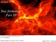
L10 From Planetesimals to protoplanets

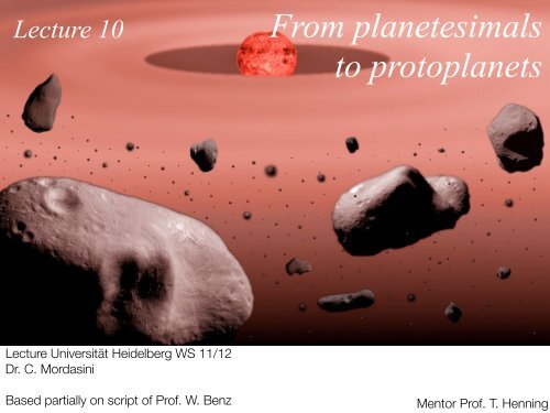
Lecture 10 

Lecture Universität Heidelberg WS 11/12 

Dr. C. Mordasini 

From planetesimals 

to protoplanets 

Based partially on script of Prof. W. Benz Mentor Prof. T. Henning

Lecture 10 overview 

1. Background: Hill radius, random velocities and feeding zone 

2. Collisional growth 

2.1 Focussing factor 

2.2 Growth rate 

2.3 Isolation mass 

2.4 Factors influencing the random velocity 

2.5 Runaway growth 

2.6 Oligarchic growth 

2.7 Orderly growth 

3. Analytical solutions 

4. Growth as a function of semimajor axis 

5. Numerical simulations

1. Hills radius, 

random velocities 

and feeding zone

Random velocities 

Random velocities 

Random velocity 

Kepler Kepler orbit orbit characterized by by 6 elements: 6 elements: 

Kepler orbit characterized by 6 elements: 

Kepler - semi-major - semi-major orbit characterized axis: by 6 elements: 

- semi-major axis: axis: a a 

- semi-major - eccentricity: - eccentricity: axis: a 

- eccentricity: e e 

- eccentricity: - inclination: e 

- inclination: 

- inclination: i i 

- inclination: i 

- longitude - longitude of ascending node: 

- longitude - longitude of ascending Ω 

of ascending of ascending node: 

node: Ω node: Ω Ω 

- longitude of perihelion: ω 

- longitude - longitude - longitude of perihelion: of perihelion: of perihelion: ω ω 

ω 

- time of passage at perihelion: τ 

- time - time - of time passage of passage of passage at perihelion: at perihelion: at perihelion: τ τ 

τ 

The Hill coordinates (x, y, z) are local coordinates rotating with Keplerian angular velocity. 

For e, i

2. Collisional growth

Growth from ~km to protoplanets 

The growth in this size range is occurring via two body collision (collisional growth). Compared 

to the earlier stages, gravity is now the dominant force, even though the gas drag still plays a 

role. Still, the growth from ~km sizes planetesimals to ~1000 km sized protoplanets is still 

difficult to study because of the following reasons: 

- Initial conditions poorly known 

- how do the first planetesimals form? 

- large number of planetesimals to follow (no direct N body) 

- 10 MEarth > 10 8 rocky bodies with R=30 km 

- long evolution time 

- 10 7 years are equivalent to 10 7 dynamical times... 

- highly non-linear with complex feed-back mechanisms 

- growing bodies play an increasing role in the dynamics 

- non-trivial physics during impacts 

- shock waves, multi-phase fluid, fracturing, etc. 

Tackle with different approaches, each with + and - points. The most simple approach is to 

study rate equations which directly give the growth rate. More complex approaches are 

statistical, Monte Carlo or (special) N-body integrations.

2.1 Focussing factor

3-body effects 

At some point, the 3-body interactions (i.e. the influence of the sun) must be accounted for. 

The two-body approximation fails in the limit of very low random velocities. This comes 

about because the encounter timescale becomes non-negligible compared to the orbital 

timescale. This causes an upper limit for the gravitational focussing factor. 

Detailed calculations (see Lissauer 1993) show that three-body stirring of the embryo 

causes a maximum value for the gravitational focussing factor Fg of the order of 10 3 -10 4 . 

Lissauer 1993 

Gravitational focussing factor including 3-body effects 

as a function of the ratio of the escape velocity to the 

planetesimal velocity dispersion (or planetesimal 

eccentricity). The dashed line indicates the two body 

approximation. 

The transition when 3-body interactions become 

relevant divides two regimes. 

Defining vH as the escape velocity at the Hill radius: 

v∞ >vH 

v∞

2.2 Growth rate

wn of constrained quantity. For this reason, the dust-to-gas ratio is 

idered varied in our simulations, and 

Mass 

takes two 

growth 

values depending 

rate 

on 

II Accretion of planetesimals 

n pro- the mid-plane temperature of the disc: fD/G for temperatures 

ration below 150 K and 1/4 fD/G for higher temperatures. In principle, 

Formation of a core 

aminar the position of the iceline should evolve because of the viscous 

, type I evolution of the disc. However, since our treatment of the plan- 

Lissauer 1993 

nearly etesimals disc is very simple, we do not take into account this Accretion rate of gas very low 

. evolution. 

Notes: 

type I We assume that due to the scattering effect of the planet, the Depletion of the feeding zone 

- the velocity dispersion of planetesimals enters only in focusing factor, but is the key factor. 

r than surface density of planetesimals is constant within the current 

anaka - the growth feeding zone rate but is larger decreases in with disks time with proportionally larger planetesimal to the mass surface densities. MZ < critical mass 

nowl- - since accreted generally (and/or ejected decrease from thewith disc) distance, by the planet. planets The feed- grow slower at large distances. 

erived - Fg can ingbe zone much is assumed more to complex extend toin a distance the three-body of 4 RH oncase. either 

al fac- side of the planetary orbit, where RH ≡ 

nDecrease that of planetesimal surface density 

rvival, 

As the protoplanet grows, the surface density of planetesimals 

ut just 

must decrease in proportion. For the assumption of accretion 

tofrom be: a feeding zone with spatially constant planetesimal surface 

density one finds for a planet with semimajor axis a 

(16) 

entum 

(17) 

xpresof 

the 

Mplanet 

1/3 

aplanet is the 

3M∗ 

Hills radius of the planet. For the inclinations and eccentricities 

of the planetesimals, we use the following prescription (P96): 

 

1 2GMplanetesimal 1 

i = 

√ , (20) 

aplanet rplanetesimal 3Ω 

where Mplanetesimal and rplanetesimal are the mass and radius of 

planetesimals, at the location of the planet, and 

 

e = max 2i, 2 RH 

 

· (21) 

aplanet 

Finally, we also take into account the ejection of planetesimals 

due to the planet, using the ejection rate given by Ida & Lin 

(2004): 

accretion rate 

ejection rate = 

02; and Bate et al. 2003) the migration prowalk, 

and the mean value of the migration 

be highly reduced, compared to the laminar 

shown by Menou & Goodman (2004), type I 

ass planets can be slowed down by nearly 

itude in regions of opacity transitions. 

ations seem to indicate that the actual type I 

le may in fact be considerably longer than 

stimated by Ward (1997) or even by Tanaka 

hese reasons, and for lack of better knowlse 

for type I migration the formula derived 

002) reduced by an arbitrary numerical faceen 

1/10 and 1/100. Tests have shown that 

r is small enough to allow planet survival, 

not change the formation timescale but just 

igration (see Sect. 3.1). 

velocity for low mass planets is taken to be: 

Γ 

net , (16) 

Lplanet 

lanet(GM∗aplanet) 

4 Vesc,disk 

, (22) 

Vsurf,planet 

1/2 is the angular momentum 

e total torque Γ is given by: 

2 Mplanet rPΩp 

αΣ,P) 

ΣPr 

M∗ Cs,P 

4 PΩ2 D/G 

below 150 K and 1/4 fD/G for higher temperatures. In principle, 

the position of the iceline should evolve because of the viscous 

evolution of the disc. However, since our treatment of the planetesimals 

disc is very simple, we do not take into account this 

evolution. 

We assume that due to the scattering effect of the planet, the 

surface density of planetesimals is constant within the current 

feeding zone but decreases with time proportionally to the mass 

accreted (and/or ejected from the disc) by the planet. The feeding 

zone is assumed to extend to a distance of 4 RH on either 

side of the planetary orbit, where RH ≡ 

p, (17) 

dlog Σ 

und velocity and αΣ ≡ dlog r . In this expres- 

P refers to quantities at the location of the 

ration, two cases have to be considered. For 

when their mass is negligible compared that 

Mplanet 

1/3 


3M∗ 



 


i = 

√ , (20) 




 


 

· (21) 

aplanet 



(2004): 



4 Vesc,disk 

, (22) 

Vsurf,planet 

where Vesc,disk = d, compared to the laminar 

u & Goodman (2004), type I 

be slowed down by nearly 

f opacity transitions. 

dicate that the actual type I 

e considerably longer than 

d (1997) or even by Tanaka 

d for lack of better knowlgration 

the formula derived 

an arbitrary numerical fac- 

100. Tests have shown that 

h to allow planet survival, 

formation timescale but just 

t. 3.1). 

mass planets is taken to be: 

(16) 

/2 is the angular momentum 

is given by: 

2 Ωp 

ΣPr 

s,P 

2 GM⊙/aplanet is the escape velocity form 

the central star, at the location of the planet, Vsurf,planet 

= 

4 PΩ2 the position of the iceline should evolve because of the viscous 

evolution of the disc. However, since our treatment of the planetesimals 

disc is very simple, we do not take into account this 

evolution. 

We assume that due to the scattering effect of the planet, the 

surface density of planetesimals is constant within the current 

feeding zone but decreases with time proportionally to the mass 

accreted (and/or ejected from the disc) by the planet. The feeding 

zone is assumed to extend to a distance of 4 RH on either 

side of the planetary orbit, where RH ≡ 

p, (17) 

dlog Σ 

αΣ ≡ dlog r . In this exprestities 

at the location of the 

s have to be considered. For 

is negligible compared that 

iven by the viscosity of the 

Mplanet 

1/3 


3M∗ 



 


i = 

√ , (20) 




 


 

· (21) 

aplanet 



(2004): 



4 Vesc,disk 

, (22) 

Vsurf,planet 

where Vesc,disk = case. Moreover, as shown by Menou & Goodman (2004), type I 

migration of low-mass planets can be slowed down by nearly 

one order of magnitude in regions of opacity transitions. 

These considerations seem to indicate that the actual type I 

migration timescale may in fact be considerably longer than 

the one originally estimated by Ward (1997) or even by Tanaka 

et al. (2002). For these reasons, and for lack of better knowledge, 

we actually use for type I migration the formula derived 

by Tanaka et al. (2002) reduced by an arbitrary numerical factor 

fI chosen between 1/10 and 1/100. Tests have shown that 

provided this factor is small enough to allow planet survival, 

its exact value does not change the formation timescale but just 

the extent of the migration (see Sect. 3.1). 

The migration velocity for low mass planets is taken to be: 

daplanet 

Γ 

= −2 fIaplanet , (16) 

dt 

Lplanet 

where Lplanet ≡ Mplanet(GM∗aplanet) 

2 GM⊙/aplanet is the escape velocity form 

the central star, at the location of the planet, Vsurf,planet 

= 

GMplanet/Rc is the planet’s characteristic surface speed, and 

1/2 is the angular momentum 

of the planet and the total torque Γ is given by: 

2 Mplanet rPΩp 

Γ = (1.364 + 0.541αΣ,P) 

ΣPr 

M∗ Cs,P 

4 PΩ2 evolution of the disc. Howev 

etesimals disc is very simple 

evolution. 

We assume that due to th 

surface density of planetesim 

feeding zone but decreases w 

accreted (and/or ejected from 

ing zone is assumed to exte 

side of the planetary orbit, w 

Hills radius of the planet. Fo 

of the planetesimals, we use 

 

1 2GMplanetesimal 

i = 

aplanet rplanetesimal 

where Mplanetesimal and rplane 

planetesimals, at the location 

 

e = max 2i, 2 

p, (17) 

dlog Σ 

where Cs is the sound velocity and αΣ ≡ dlog r . In this expression, 

the subscript P refers to quantities at the location of the 

planet. 

For type II migration, two cases have to be considered. For 

low mass planets (when their mass is negligible compared that 

of the disc) the inward velocity is given by the viscosity of the 

disc. As the mass of the planet grows and becomes comparable 

RH 

 

· 

aplanet 

Finally, we also take into ac 

due to the planet, using the 

(2004): 



 

Vesc,disk 

Vsurf,planet 

where Vesc,disk = Ejection 

As the mass of the protoplanet increases, it becomes at some point massive enough to also 

eject planetesimals form the nebula. 

2 GM⊙/ 

the 

 

central star, at the loc 

GMplanet/Rc is the planet’s 

Rc is the planet’s capture rad

2.3 Isolation mass

2.4 Factors influencing the 

random velocity

Planetesimal random velocities 

In recent years, considerable effort has been devoted to understand the collisional growth of 

a swarm of planetesimals, and in particular the random velocities as this sets the growth 

regime: runaway, oligarchic, orderly. The key ingredients are: 

1) viscous stirring through gravitational scattering (increase of random velocities) 

-among the planetesimals 

-by the protoplanet 

2) stirring by inelastic collisions 

3) damping due to dissipation in inelastic collisions 

4) damping due to gas drag 

5) dynamical friction: energy transfer from large to small bodies 

Of all these processes, the last one is particularly important. Indeed, dynamical friction tends 

to establish energy equipartition between bodies of different sizes. Hence, large bodies move 

slowly and have large escape velocity thus the collisional cross section can become quite 

large. This effect by which the larger bodies grow larger and larger at the expenses of 

smaller ones is called runaway growth.

Dynamics of planetesimals 43 

Figure 1. Snapshots of the planetesimal system on the a-e (left) and a-i (right) planes at 

The plot shows snapshots t = 0 year (top) and of 10000 at t=0 year (bottom). and 10000 years on the a-e and a-i planes of the 

planetesimals. The eccentricities and inclinations of most planetesimals significantly increase in 

10000 years. On average, the increase of e is larger than that of i. The distributions of e and i 

relax into a Rayleigh distributions. We also see the diffusion of planetesimals in a, which is the 

result of random walk in a due to two-body scattering. 

Figure 2. Time evolution of σe (solid) and σi (dashed). 

Viscous stirring 

Viscous stirring is the process in which the velocity dispersions of planetesimals increases 

due to two-body encounters. 

1) Viscous stirring among planetesimals 

Kokubo 2005 

2) Viscous stirring by the protoplanet 

Text 

Text 

Direct N-body simulation of 

1000 equal-mass (m = 10 24 g) 

planetesimals distributed in a 

ring at a = 1AU with width ∆a 

= 0.07AU. 

The “heating of neighbor planetesimals by a protoplanet” eventually leads to the decrease of 

the growth rate of the protoplanet, as in increases the random velocity of the planetesimals.

Viscous stirring II 

The timescale of viscous stirring of a planetesimals with eccentricity e by protoplanets of mass M 

is given by (Ida & Makino 1993) 

where ns,M is the surface number density of protoplanets, ΣM/M.

Gas damping of velocities 

The process of damping of the random velocities by gas drag is basically the same as we have 

seen earlier for smaller particles, although the drag regime is now different (Kn>>1, hydrodynamic 

regime) and thus scales as v 2 : 

Damping is good for fast growth, as it decreases the planetesimal random velocities which 

are increased by viscous stirring, leading to an equilibrium. As in the last lecture, we estimate 

the damping timescale as 

Here we have approximated the random velocity as 

Gas damping occurs on a shorter timescale for smaller planetesimals. For too small 

planetesimals however, fast radial drift comes back as a potentially very dangerous mechanism. 

If the planetesimal random velocities are strongly damped, the system evolves into the shear 

dominated regime with a very thin disk of planetesimals. This means that growth becomes a 

2D problem (instead of a 3D) with high collisional probability and large focussing factors. This 

leads to a very large growth rate.

Dynamical friction II 

Direct N-body integration of a protoplanet with mass M = 100 m embedded in a swarm of 

planetesimals. The initial orbital elements of the protoplanet are aM =1AU and eM =iM =0.01. 

44 Kokubo 

44 Kokubo 

Kokubo 2005 

Figure 3. Snapshots of the planetesimal system on the a-e(left) and a-i (right) planes at t =0 

year (top) and 3000 year (bottom). The large circle indicates the protoplanet. 

Figure 3. Snapshots of the planetesimal system on the a-e(left) and a-i (right) planes at t =0 

year (top) and 3000 year (bottom). The large circle indicates the protoplanet. 

The eM and iM of the 

protoplanet decrease to almost 

0 in 3000 years while the 

semimajor axis is nearly 

constant. On the other hand, 

the e and i of the neighbor 

planetesimals are raised by 

reaction (viscous stirring). 

The V-like structure around the protoplanet on the a-e plane corresponds to the constant Jacobi 

energy curve. 

Time evolution of eM (solid) and iM 

(dashed) of the protoplanet. The 

protoplanet ends on a non-inclined, 

circular orbit.

2.5 Runaway growth

Runaway growth 

The first stage of collisional growth of planetesimals to protoplanets is thought to occur in the 

so called runaway growth regime (Wetherill & Steward 1980). In this regime, the random 

velocity of the planetesimals is determined solely by planetesimal-planetesimal scattering, and 

focussing is strong. 

Runaway growth means that larger planetesimals grow more rapidly than smaller ones and the 

mass ratio between them increases monotonically. It is caused by the effect of the energy 

equipartition between large and small planetesimals, in other words, dynamical friction on 

protoplanets by small planetesimals. 

Runaway growth mechanism 

0)spontaneous formation of one body (slightly) more massive than the other ones. 

1)dynamical friction/equipartition of energy means that the e and i of the big body become small. 

2)the e and i of the small bodies are (at least in the early stage) not affected/increased. 

3)the relative velocity between the big and the small body becomes small. 

4)at the same time, vesc of the big body increase due to its increase in mass. 

5)the gravitational focussing factor of the big body thus becomes 

The small bodies have in comparison a much smaller Fg. 

6)the runaway body grows faster than the planetesimals, consuming all planetesimals in the 

feeding zone (in principle). It decouples from the mass distribution of the small ones. 

We note that runaway growth is clearly a strongly nonlinear process.

Formation of a few large bodies well 

separated (~ 5 Rhills). Note their low 

eccentricity 

Runaway growth III 

Collisional evolution of s swarm of 4'000 equal mass bodies (m=3×10 23 g). Perfect accretion is 

assumed. A discrete body Monte Carlo method is used for the simulation. 

Benz et al. 

largest body 

gravitational encounters → equipartition of energy → runaway growth 

average 

The largest body is growing faster than the 

average body. It decouples from the 

background planetesimals.

2.6 Oligarchic growth

Oligarchic growth 

Originally, it was thought that runaway growth might continue until the isolation masses are 

reached. Then it was understood (Ida & Makino 1993) that this is incorrect. They showed that 

after the runaway bodies have grown to a certain size, the growth mode changes into the so 

called oligarchic growth. The big bodies are now called oligarchs. This is due to a feedback 

of the big bodies onto the random velocities of the small one (viscous stirring). 

Initially, the dynamics of the planetesimal disk is not affected by the presence of the bigger 

protoplanets, and their growth proceeds very rapidly in the runaway regime. Later however, 

when the embryo starts being dynamically important its accretion slows down. As runaway 

growth proceeds, the runaway bodies become detached from the continuous mass 

distribution and they become the scattering center. They heat up the random velocities of the 

small bodies. 

Clearly, this reduces the gravitational focussing factor 

As a result, more massive bodies grow more slowly than the less massive ones (similar to 

orderly growth, cf below), but protoplanets still grow faster than planetesimals in their 

surroundings (similar to runaway growth). Accretion in the oligarchic regime is slower than in 

the runaway regime but faster than in the orderly regime.

Ida & Makino 1993 studied when the feedback of the big body on the random velocities of the 

planetesimals growth–oligarchy becomes important, i.e. transition when the takes transition place from at runaway the point to oligarchy where the occurs. 

Modern view: Once the protoplanet reaches a 

stirring 

certain 

power 

mass, 

of big 

then 

bodies 

run-away 

first exceeds 

stops 

that 

and 

of 

orderly 

the small bodies, 

i.e., 

‘oligarchic growth’ phase starts: 

2ΣMM >Σmm, (1) 

They found this analytical criterion 

where 

stirring rate of small bodies is determined by the same big body 

that accretes them. Oligarchic Runaway growth growth has passedIIinto oligarchy 

(Kokubo From & Ida run-away 1998). to oligarchic growth 

Ida & Makino (1993) have argued that the runaway 

2" M M > " m m 

(Ida & Makino 1993) 

where ΣM is the surface density of big bodies of mass M and Σm 

M = Mass of large (dominating) bodies 

! M = Surface density of large (dominating) bodies 

m ! = Mass of small planetesimals 

! m = Surface density of small planetesimals 

Typically this is reached at 10-6 ..10-5 M". 

From here on: gravitational influence of protoplanet 

determines random velocities, not the self-stirring of 

the planetesimals. ‘Oligarchic growth’. 

10-2 that of the small bodies. Equation (1) canbetransformedinto 

aradius,Rrg/oli, indicatingtheturnoverfromrunawaygrowth 

into oligarchy (see below, Equation (4)). Many works have 

adopted Equation (1)asthestartoftheiroligarchiccalculations 

(e.g., Thommes et al. 2003; Ida&Lin2004; Chambers2006, 

2008; Fortier et al. 2007;Brunini&Benvenuto2008;Miguel& 

Brunini 2008; Mordasini et al. 2009). 

In this Letter, we will refine the criterion of Ida & Makino 

(1993)andpresentanewexpressionforRrg/oli Mearth. 

(Equation (13)). 

The result of Ida & Makino correspond to a transition 

from runaway already at small masses, of order 10-6 to 10-5 Mearth. More recent calculation of Ormel et al. 

2011 indicate a transition at masses of order 10-3 to 

L103 

our 

tim 

sim 

Rtr 

imp 

T 

ma 

wit 

and 

vel 

gra 

v 2 esc

Oligarchic growth IV 

In the oligarchic growth stage, the random velocity (eccentricity e and inclination i) of the 

planetesimals is raised by viscous stirring by the protoplanets and is damped by gas drag. 

The planetesimals attain an equilibrium RMS eccentricity when gravitational perturbations due 

to the protoplanets are balanced by dissipation due to gas drag. Following Ida and Makino 

(1993), one obtains the equilibrium eccentricity by equating the viscous stirring timescale due 

to a protoplanet of mass M, with the eccentricity damping timescale due to gas drag. 

One finds (Thommes et al. 2003)

2.7 Orderly growth

Orderly growth 

Once the gaseous nebula is dispersed (after ~10 Myrs), and all planetesimals have been 

accreted into oligarchs, no mechanisms (gas damping, viscous friction) exist any more to 

damp the random velocities of the big bodies. Gravitational scattering then increases the 

random velocities to v~vesc. This means that the gravitational focussing factor Fg becomes ~1. 

The collisional cross section is thus reduced to the geometrical cross section. Growth in this 

regime is very slow. Growth of velocity dispersion in the disk is dominated by the 

protoplanets, and gravitational focusing is weak. 

With Fg =1, the master equation becomes 

or in relative terms 

This means that the growth rate decreases with increasing mass. Bigger bodies grow slower. 

This is the same as in the oligarchic regime. However, Fg is much larger in the oligarchic 

regime than in the orderly growth regime. 

Orderly growth is the final regime for planet growth, at least in the inner solar system.

3. Analytical solutions

August 3, 2011 

Analytical solutions of the master equation 

August August3, 3, 2011 2011 

1 Task A 

1 Task A 

For orderly growth, and for runaway, analytical solutions to the growth equation can be found. 

We will work using the radius R, instead of the mass M, as the radius directly enters in the 

cross section. 1.1We No assume focussing, that planets ΣP constant are spherical and have a constant density. Then we 

can always In convert this problem, radius as into well mass as in all and other vice ones, versa. we will work using theradiusR, 

instead of the mass M, astheradiusdirectlyentersinthecrosssection.We 

1) Orderly growth assume that (Fg=1), planets constant are spherical planetesimal and have asurface constantdensity density. Then we can 

The constant always surface convert density radiusapproximation into mass and vice should versa. be fine as long as M

3 Task C 

Analytical solutions II 

2) Orderly growth (Fg=1), decreasing planetesimal surface density 

The accretion of the planet from a feeding zone of with BRH leads to a 

The accretion decreaseof of the theplanet surface from density a feeding as zone of width B RH leads to a decrease of the surface 

density as 

ΣP (t) =Σ0 − M(t) 

(10) 

2πaBRH 

where Σ0 is the initial planetesimal surface density. We can express RH in 

where Σ0 terms is the of initial the planetesimal radius of the planet, surface density. 2 We can express RH in terms of the radius 

of the planet, 

1/3 4πρ 

RH = Ra. (11) 

9M∗ 

With these equations, we can express ΣP (t) asafunctionofR(t), and find 

ΣP (R) =Σ0 − k3R2 = k2 − k3R2 . 

3.1 No focussing, ΣP variable 

Plugging ΣP (R) backinourmasterequationfordR(t)/dt, wenowgeta 

differential equation 

dR 

dt = k1(k2 − k3R 2 )=a − bR 2 

where Σ0 is the initial planetesimal surface density. We can expres 

terms of the radius of the planet, 

1/3 4πρ 

RH = Ra. 

9M∗ 

With these equations, we can express ΣP(t) as a function of R(t), and find 

With these equations, we can express ΣP (t) asafunctionofR(t), 

ΣP (R) =Σ0 − k3R 

(12) 

where we have defined a number of constants for simple algebra. Re-arranging 

to separate the variables, we have 

dR 

= dt. (13) 

a − bR2 2 = k2 − k3R2 . 


Plugging ΣP (R) backinourmasterequationfordR(t)/dt, weno 


dR 

dt = k1(k2 − k3R 2 )=a − bR 2 



1/3 4πρ 

RH = Ra. (11) 

9M∗ 


ΣP (R) =Σ0 − k3R 

Plugging ΣP(R) back in our master equation for dR(t)/dt for Fg=1, we now get a differential 

equation 

where we have defined a number of constants for simple algebra. Re-a 


2 = k2 − k3R2 . 




dR 

dt = k1(k2 − k3R 2 )=a − bR 2 



1/3 4πρ 

RH = Ra. (11) 

9M∗ 


ΣP (R) =Σ0 − k3R 

(12) 

where we where have defined we havea defined number a number of constants of constants for simple for simple algebra. algebra. Re-arranging Re-arranging to separate the 

variables, we to separate have the variables, we have 

dR 

= dt. (13) 

a − bR2 2 = k2 − k3R2 . 




dR 

dt = k1(k2 − k3R 2 )=a − bR 2 

(12) 

where we have defined a number of constants for simple algebra. Re-arranging 


dR 

= dt. (13) 

a − bR2 The right side The is trivial right to side integrate, is trivialthe to left integrate, we rewrite the left as 

we rewrite again as

= dt. (13) 

Analytical a − bRsolutions 2 

III 

The right side is trivial to integrate, the left we rewrite again as 

 

1 1 

b c2 1 

dR = 

− R2 bc arctanh 

 

R 

(14) 

c 

where c2 = a/b. Thisintegralcanforexamplebelookedupinintegraltables, 

and we give the result on the right. Using again a radius R0 at t =0,we 

finally get 

√ 

3Ω 

k1 = 

(15) 

8ρ 

k2 = Σ0 (16) 

1/3 2/3 

2M∗ ρ 

k3 = 

3π a2 a − bR 

The right side is trivial to integrate, the left we rewrite again as 

 

1 1 

b c 

(17) 

B 

⎡ 

⎛ ⎞⎤ 

2 1 

dR = 

− R2 bc arctanh 

 

R 

(14) 

c 

where c2 = a/b. Thisintegralcanforexamplebelookedupinintegraltables, 

and we give the result on the right. Using again a radius R0 at t =0,we 

finally get 

√ 

3Ω 

k1 = 

(15) 

8ρ 

k2 = Σ0 (16) 

1/3 2/3 

2M∗ ρ 

k3 = 

3π a2 (17) 

B 

⎡ 

⎛ 

⎞⎤ 

 

k2 

k3 

R(t) = tanh k2k3t +arctanh⎝ 

⎠⎦ 

(18) 

where c 2 = a/b. Using again a radius R0 at t = 0, we finally get 

⎣k1 

 

k3 

 

1.2 Strong k2 

R(t) focussing, = tanh ⎣k1 

ΣP constant 

k3 

k2k3t +arctanh 

⎝ 

 

R0 

k2k3 

R0 

k2 

1.2 Strong focussing, ΣP constant 

We note that we can write the escape velocity as 

We note that we can write 3 the escape velocity as 

3) Runaway growth (Fg>>1), constant planetesimal surface density 

v 2 esc = 8 

dR 

dt 

⎠ 

⎦ (18) 

3 

v 2 esc = 8 

3 GπρR2 We note that we can write the escape velocity 3as . (5) 

In the strong focussing case, In thevesc/v strong≫ focussing 1, therefore case, vesc/v the differential ≫ 1, therefore equation the differential for R is equation now of the 

for R is now (approximately) of the form 

form (approximately) 

2 

= k1R (6) 

GπρR2 . (5) 

In the strong focussing case, vesc/v ≫ 1, therefore the differential equation 

for R is now (approximately) of the form 

dR 2 

= k1R (6) 

dt 

where k1 is where again k1 another is againconstant. another constant. We separate We separate the variables the variables and write 

and write 

where k1 is again another constant. We separate the variables and write

where k1 is again another constant. We separate the variables and write 

dt 

Analytical solutions IV 

where k1 is again another constant. We separate the variables and write 

dR 

R2 = k1dt. (7) 

Solving this differential equation, plugging in the parameters, and re-arranging 

gives 

3R0v 

R(t) = 

2 

3v2 − √ Solving this differential equation, plugging in the parameters, and re-arranging gives 

gives 

3R0v 

R(t) = 

. (8) 

3GπR0ΣP Ωt 2 

. (8) 

2 Task B 

dR 

R2 = k1dt. (7) 

Solving this differential equation, plugging in the parameters, and re-arranging 

2 Task B 

3v 2 − √ 3GπR0ΣP Ωt 

Clearly, R will approach infinity in a finite amount of time for this case. 

3.2 Strong focussing, ΣP variable 

From the last equation it is clear that R approaches infinity when the denominator 

becomes zero. This happens at a time 

√ 

3/2 2 3a v 

t = 

G3/2√ . (9) 

M∗πR0ΣP 

This is a consequence of the fact that the bigger the planet is, thefasterit 

grows, and the supply of planetesimals is assumed to be infinite (ΣP =cst.). 

3 Task C 


decrease of the surface density as 

ΣP (t) =Σ0 − M(t) 

From the last equation it is clear that R approaches infinity when the denominator 

becomes zero. This happens at a time 

√ 

3/2 2 3a v 

t = 

G 

(10) 

2πaBRH 

3/2√ 4) Runaway growth (Fg>>1), decreasing planetesimal surface density 

3.2 Strong focussing, ΣP variable 

Here we Here can we combine can go the backcase to the of case strong of strong focussing focussing and ΣP andconstant, ΣP constant, but use but ΣP(R) as derived 

above for use scenario ΣP (R) asderivedabove. 2. This leads to Thisleadstoadifferential a differential equation of equation the formof 

the form 

. (9) 

dR M∗πR0ΣP 

dt 

This is a consequence of the fact that the bigger the planet is, thefasterit 

grows, and the supply of planetesimals is assumed to be infinite (ΣP =cst.). 

3 Task C 


decrease of the surface density as 

= k1R 2 (k2 − k3R 2 ). (19) 

We separate the variables and come to an equation 

 

1 

R2 (a2 − R2 ) dR = k3k1t + C2 

(20) 

with a2 = k2/k3, andC2is the integration constant. In integral tables we 

find that the integral is equal to 

 

1 R 

arctanh − 

a3 a 

1 

a2 Here we can go back to the case of strong focussing and ΣP constant, but 

use ΣP (R) asderivedabove. Thisleadstoadifferential equation of the form 

dR 

dt 

Separating the variables yields 

(21) 

R 

= k1R 2 (k2 − k3R 2 ). (19) 


 

1 

R2 (a2 − R2 ) dR = k3k1t + C2 

(20) 



 

1 R 

arctanh − 1 

with a 

(21) 

2 3.2 Strong focussing, ΣP variable 

Here we can go back to the case of strong focussing and ΣP constant, but 

use ΣP (R) asderivedabove. Thisleadstoadifferential equation of the form 

dR 

dt 

= k2/k3, and C2 is the integration constant. The integral is equal to 

= k1R 2 (k2 − k3R 2 ). (19) 


 

1 

R2 (a2 − R2 ) dR = k3k1t + C2 

(20) 



 

1 R 

arctanh − 

a3 a 

1 

a2 (21) 

R 

M(t)


This finally leads to the solution 

Analytical solutions V 

 

1 R 

arctanh 

a3 This finally leads us to the solution 

k1 = πGΩ 

√ 3v 2 

a 

− 1 

a2R (21) 

(22) 

k2 = Σ0 (23) 

1/3 2/3 ρ 

k3 = 

C2 = 

k3k1t + C2 = 

 

2M∗ 

3π 

3/2 k3 

k2 

3/2 k3 

k2 

a 2 B 

arctanh 

arctanh 

⎛ 

⎝ 

⎛ 

⎝ 

⎞ 

k3 

R0 

⎠ − 

k2 

k3 

k2R0 

k3 

k2 

R 

⎞ 

⎠ − k3 

(24) 

(25) 

. (26) 

k2R 

In the last line, we cannot directly solve analytically for R, incontrasttothe 

three previous cases. But we can specify the parameters, and t, andthen 

solve the implicit equation numerically for example with bisection. 

In the last line, we cannot directly solve analytically for R, in contrast to the three previous cases. 

But we can specify the parameters, and t, and then solve the equation numerically for R using for 

example the bisection method. 

4 Task D 

With the parameters mentioned in the exercise, we find an M(t) forthefour 

cases shown in the following figures. We see that for both cases whereΣ is 

4

Mass [Earth Masses] 

10 

1 

0.1 

0.01 

0.001 

Analytical solutions VI 

With these equations, we can study the growth of protoplanets at 1 AU and at 5 AU for the two 

regimes. We assume a density of 3.2 g/cm 3 , a planetesimal radius of 100 km, an initial 

protoplanet radius of 1000 km, a solar mass star, B=10, and an initial planetesimal surface 

density at 1 AU of 7 g/cm 2 (MMSN) and of 10 g/cm 2 (ca. 4 x MMSN) 5 AU. For the random 

velocity of the planetesimals we assume self-stirring only, i.e. 

1 AU, MMSN 

Isolation Mass 

No focussing, Sigma cst 

Strong focussing, Sigma cst 

No focussing, Sigma var 

Strong focussing, Sigma var 

100 1000 10000 100000 1e+06 1e+07 1e+08 1e+09 1e+10 

Time [yr] 


1000 

100 

10 

1 

0.1 

0.01 

0.001 

5.2 AU, 4 x MMSN 

Isolation Mass 





1000 10000 100000 1e+06 1e+07 1e+08 1e+09 1e+10 

Time [yr] 

Note 

-At early times, the cases with constant and decreasing ΣP are similar. 

-For the cases with decreasing ΣP, the isolation mass is eventually reached. 

-In runaway, isolation is reached in ~10 5 and 10 6 yrs at 1 and 5 AU, respectively 

-In orderly growth, isolation is reached in ~10 8 and 10 10 yrs at 1 and 5 AU, respectively.

4. Growth as a function of 

semimajor axis

5 Task E 



1000 

100 

10 

1 

0.1 

0.01 

1000 

100 

10 

1 

0.1 

0.01 

Growth as function of semimajor axis 

We can also use the analytical results to study the growth as a function of distance. 

0.1 Myr, 4 x MMSN 

0.01 0.1 1 10 100 

a [AU] 

10 Myr, 4 x MMSN 

Isolation mass 





0.01 0.1 1 10 100 

a [AU] 








1000 

100 

10 

1 

0.1 

0.01 

1000 

100 

10 

1 

0.1 

0.01 


0.01 0.1 1 10 100 

a [AU] 







0.01 0.1 1 10 100 

a [AU] 






Figure 3: Runaway and orderly growth as a function of semimajor axis, for 

t =105 , 106 , 107 and 108 Giant planet formation at large distances is a race against the clock, as we need to build up a 

∼10 MEarth core during the lifetime of the protoplanetary disk (∼10 Myrs). But growth is slow at 

large distances, even in runaway. years. Orderly growth is completely hopeless...

The problem of Uranus and Neptune 

We see that even in a nebula several times more massive than the MMSN, not much growth 

happens outside of 10 AU during the first 10 Myr, even in runaway. 

The slower character of the planetesimal accretion in the more realistic oligarchic regime leads 

to a considerable increase of the protoplanetary formation timescale compared with the 

simple runaway accretion picture. This makes the timescale problem even more severe. 

The apparent inability to accrete massive bodies within 10 Myrs in the trans-saturnian region 

presents a definite puzzle to the understanding of the formation of the Solar System. Both ice 

giants contain about 1 to 3 Earth masses of H/He, so they must have grown to their mass 

while the nebula was still around. But we know that gas disks don’t life longer than ~10 Myrs 

(mean is rather only 3 Myrs). 

Even for the cores of Jupiter and Saturn, in the oligarchic regime, growth to 10 Mearth in

Inner solar system 

Many 0.01 to 0.1 MEarth protoplanets. 

During the presence of the gas disk, growth stalled at this mass, as gas damping hinders 

development of high eccentricities (i.e. mutual collision between these bodies). 

Outer solar system 

Outcome of the growth process 

A few 1 to 10 MEarth protoplanets. 

If formed quickly and massive enough (M>ca 10 MEarth), potential to accrete gas to form a 

giant planet.

5. Numerical simulations

This method is based on the following principles: Monte Carlo (probabilistic), particle-in-a-box 

(statistical); discrete (masses); adaptive (superparticles) 

The following physical effects are included: 

•Viscous stirring 

increase of random velocities (e, i) 

•Gas drag damping 

•Collisions 

•Dynamical friction 

energy equipartition 

•Annulus at 1 AU 

•7 km initial size 

•Dot size: total mass in size bin 

•Color: relative random velocity in 

units of v/vH (vH=Ω RH) 

Ormel et al. 2010 

Monte Carlo method

-early phase: 

runaway growth. 

low random velocities 

fast growth 

big bodies decouple 

-later phase: 

oligarchic growth. 

big bodies “heat” smaller 

higher random velocities 

slower growth 

big bodies grow in lockstep 

-finally: 

isolation mass 

oligarchs separated by a few RH 

Monte Carlo method II 

Ormel et al. 2010

Questions?

L10 From Planetesimals to protoplanets

You also want an ePaper? Increase the reach of your titles

Delete template?

Save as template?