Answer Key - Mypage

E724 Financial Econometrics (Spring 2013) Problem Set 3
Instructor: Prof. Joon Park
By Ye Lu
February 16, 2013
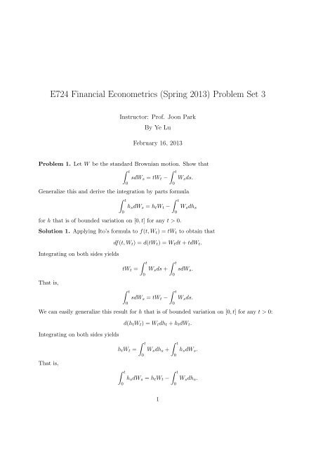
Problem 1. Let W be the standard Brownian motion. Show that
t
t
sdWs = tWt − Wsds.
Generalize this and derive the integration by parts formula
t
t
hsdWs = htWt − Wsdhs
for h that is of bounded variation on [0, t] for any t > 0.
0
0
Solution 1. Applying Ito’s formula to f(t, Wt) = tWt to obtain that
Integrating on both sides yields
That is,
df(t, Wt) = d(tWt) = Wtdt + tdWt.
t t
tWt = Wsds + sdWs.
0
t
t
sdWs = tWt − Wsds.
0
We can easily generalize this result for h that is of bounded variation on [0, t] for any t > 0:
d(htWt) = Wtdht + htdWt.
Integrating on both sides yields
t t
htWt = Wsdhs + hsdWs.
That is,
0
t
t
hsdWs = htWt − Wsdhs.
0
1
0
0
0
0
0
0

2
Problem 2. Let W be the standard Brownian motion, and suppose h : [0, ∞) → R is continuous.
Show that
t
t
hsdWs ∼ N 0, h 2
sds .
Generalize this and obtain the joint distribution of
t t
hsdWs, ksdWs
0
0
where k : [0, ∞) → R is another continuous function. Use this result to find the joint distribution
of
t
Wt, sdWs .
Note that Wt = t
0 dWs.
Solution 2. (i) Firstly we show that
t
t
hsdWs ∼ N 0,
0
0
0
0
0
h 2
sds .
Let Pt = t
0 hsdWs, it suffices to show the moment generating function of Pt has the
following form:
E(e uPt
) = E exp(u
t
0
hsdWs)
= exp µu + 1
2 σ2u 2
1
= exp
2 u2
t
0
h 2
sds ,
which is equivalent to showing that
t
E exp(u hsdWs −
0
1
2 u2
t
h
0
2
sds) = 1. (1)
Denote Xt = exp u t
0 hsdWs − 1
2u2 t
0 h2
sds and note that it is a martingale. Hence
E(Xt) = E(X0) = E exp u
which gives us equation (1) as desired.
0
0
hsdWs − 1
2 u2
Below we show that X = (Xt) is a martingale process. Notice that
t
Xt = exp u hsdWs − 1
2 u2
t
h 2
sds
0
0
0
0
h 2
sds = E(e 0 ) = 1,

E724 Financial Econometrics (Spring 2013) Problem Set 3 3
with X0 = 1 is a generalized geometric Brownian motion which is the solution to the
stochastic differential equation
dXt = uhtXtdWt. (2)
To see this, we apply Ito formula and then plug in (2) to obtain
d ln Xt = dXt
Xt
Integrating on both sides of (3) yields
and thus
With X0 = 1,
From (2) we can see that
t
ln Xt − ln X0 = u
Xt = X0 exp u
Xt = exp u
− 1 d[X]t
2 X2 t
= uhtdWt − 1
2 u2 h 2 t dt (3)
t
t
0
0
0
Xt = X0 +
hsdWs − 1
2 u2
hsdWs − 1
2 u2
hsdWs − 1
2 u2
t
t
h 2 sds,
t
0
t
uhsXsdWs
0
0
0
h 2
sds .
h 2
sds .
where the RHS of (4) is a constant plus an Ito integral, which turns out to be a martingale.
This shows that (Xt) is a martingale.
Given Pt follows normal distribution, then by computing its mean and variance:
we have
t
E(Pt) = E hsdWs = 0
0
Var(Pt) = E (Pt) 2 t
= E ([P ]t) = h 2 sds,
t
Pt =
0
hsdWs ∼ N 0,
t
0
0
h 2
sds .
(4)

4
(ii) Another way to show
t
Pt =
0
hsdWs ∼ N 0,
t
0
h 2
sds .
is given as follows. Let Pnt = n hti−1 (Wti i=1 − Wti−1 ). By definition of Ito integral,
This implies
Pnt →p Pt as πn → 0.
Pnt →d Pt as πn → 0. (5)
By the properties of Brownian motion, we know that
n
Pnt ∼ N 0, h 2 ti−1 (ti
− ti−1)
i=1
Then the moment generating function of Pnt is given by
Mn(u) = E e uPnt
1
= exp
2 u2
n
h
i=1
2 ti−1 (ti
− ti−1)
1
→ exp
2 u2
t
h 2
sds ≡ M(u), as πn → 0. (6)
0
Since Xn →d X if and only if moment generating function of Xn converges to moment
generating function of X, from (5) and (6) it follows that Pt
must have moment generating
function M(u) in (6). That is Pt ∼ N 0, t
0 h2
sds as desired.
(iii) Generalizing the above result, denote
t t
′
Qt = hsdWs, ksdWs ,
0
and Qt follows multivariate normal distribution with mean and variance given by
t t
′
E(Qt) = E hsdWs, ksdWs = (0, 0)
0
0
′ ;
Var(Qt) = E QtQ ′
t
t = E ([Q]t) = 0 h2 t
sds 0 hsksds
.
0
t
0 hsksds
(iv) Specifically, the joint distribution of
t t t
Wt, sdWs = 1dWs, sdWs
0
0
0
t
0 k2 sds

E724 Financial Econometrics (Spring 2013) Problem Set 3 5
is
0 t
N , 0
0
ds
t
0 sds
t
0 sds t
0 s2ds
= N
0
,
0
t 1/2t 2
1/2t 2 1/3t 3
.
Problem 3. Let Bt = (Bit) be a vector Brownian motion with variance Σ = (σij). Show that
[Bi, Bj]t = σijt
for all i and j. In particular, [Bi, Bj]t = 0 for all t ≥ 0, if σij = 0.
Solution 3. We can solve this problem by two ways.
(i) We can show that n
Bi,tk k=1 − Bi,tk−1 Bj,tk − Bj,tk−1 →L2 σijt as πn → 0:
n
2
E Bi,tk − Bi,tk−1 Bj,tk − Bj,tk−1 − σijt
= E
= E
=
=
=
k=1
n
k=1
n
n
k=1
− 2
Bi,tk − Bi,tk−1
Bj,tk
− Bj,tk−1
Bi,tk − Bi,tk−1 Bj,tk − Bj,tk−1
k=1
Bi,tk 2
E − Bi,tk−1 Bj,tk − Bj,tk−1
n
σij(tk − tk−1)E Bi,tk
k=1
n
(σiiσjj + 2σ 2 ij)(tk − tk−1) 2 − 2
k=1
n
k=1
(σiiσjj + σ 2 ij)(tk − tk−1) 2
≤ (σiiσjj + σ 2 ij) max
1≤k≤n |tk − tk−1|
− Bi,tk−1
− σij(tk − tk−1) 2
− σij(tk − tk−1) 2
2
Bj,tk
− Bj,tk−1
n
σ 2 ij(tk − tk−1) 2 +
k=1
n
(tk − tk−1)
k=1
+
n
k=1
n
k=1
σ 2 ij(tk − tk−1) 2
σ 2 ij(tk − tk−1) 2
= t(σiiσjj + σ 2 ij) max
1≤k≤n |tk − tk−1| → 0, as πn → 0.
Therefore n
Bi,tk k=1 − Bi,tk−1 Bj,tk − Bj,tk−1 →p σijt as πn → 0, thus
[Bi, Bj]t = plim
n
Bi,tk − Bi,tk−1
πn→0
k=1
Bj,tk
− Bj,tk−1
= σijt.

6
(ii) Since Bt = (Bit) is a vector Brownian motion with variance Σ = (σij), it can be written
as
Bt = Σ 1/2 Wt
where Wt = (Wit) is a vector of independent standard Brownian motions W1t, W2t, · · · , Wnt.
Let
It then follows that
n
[Bi, Bj]t =
A = Σ 1/2 = (aij), and hence AA = AA ′ = Σ = (σij). (7)
= 1
4
= 1
4
k=1
k=1
aikWk,
n
k=1
ajkWk
t
n
n
aikWk + ajkWk −
k=1
k=1 t
1
n
n
aikWk −
4
k=1
k=1
n
(aik + ajk)Wk − 1
n
(aik − ajk)Wk
4
t
k=1
= 1
n
(aik + ajk)
4
k=1
2 [Wk]t − 1
n
4
k=1
= 1
n
(aik + ajk)
4
k=1
2 − (aik − ajk) 2 [Wk]t
= 1
n
4aikajk[Wk]t
4
k=1
n
=
k=1
(aik − ajk) 2 [Wk]t
t
ajkWk
aikajkt = σijt (9)
where (9) is obtained from (7), and (8) is obtain by the fact that
[X, Y ]t = 1
4 ([X + Y ]t − [X − Y ]t) .
Problem 4. Prove directly from the definition of Ito integrals that
t
t
sdMs = tMt − Msds,
0
where M is a continuous martingale. Can this formula be generalized to
t
t
f(s)dMs = f(t)Mt Msdf(s)
0
for any function f that is of bounded variation over any compact interval?
0
0
t
(8)

E724 Financial Econometrics (Spring 2013) Problem Set 3 7
Solution 4. By definition of Ito integral,
Similarly,
t
0
t
0
sdMs = plim
πn→0
f(s)dMs = plim
πn→0
n
ti−1(Mti
i=1
n
ti−1Mti
− Mti−1 )
= plim
− tiMti + tiMti − ti−1Mti−1
πn→0
i=1
n
= plim (tiMti − ti−1Mti−1 ) − (tiMti − ti−1Mti )
πn→0
i=1
n
n
= plim (tiMti − ti−1Mti−1 ) − plim Mti
πn→0
πn→0
i=1
i=1
(ti − ti−1)
t t
= d(sMs) − Msds
0
t
0
= tMt − Msds.
0
n
f(ti−1)(Mti − Mti−1 )
i=1
n
f(ti−1)Mti
= plim
− f(ti)Mti + f(ti)Mti − f(ti−1)Mti−1
πn→0
i=1
n
= plim (f(ti)Mti − f(ti−1)Mti−1 ) − (f(ti)Mti − f(ti−1)Mti )
πn→0
i=1
n
n
= plim (f(ti)Mti − f(ti−1)Mti−1 ) − plim Mti
πn→0
πn→0
i=1
i=1
(f(ti) − f(ti−1))
t
t
= d(f(s)Ms) − Msdf(s)
0
t
0
= f(t)Mt − Msdf(s),
0
for any function f that is of bounded variation over any compact interval.
Problem 5. Check whether the following processes X are martingales with respect to the
filtration (Ft) generated by the standard Brownian motion W (for (a) - (c)), or the two
independent standard Brownian motions W and V (for (d)).
(a) Xt = Wt + 4t
(b) Xt = W 3 t − 3tWt

8
(c) Xt = t 2 Wt − 2 t
0 sWsds
(d) Xt = WtVt
Solution 5. (a) Note that for s < t,
E (Xt|Fs) = E (Wt + 4t|Fs) = Ws + 4t = Xs.
Therefore X is not a martingale with respect to Ft.
(b) Apply Ito formula to obtain that
Then
dXt = (3W 2 t − 3t)dWt − 3Wtdt + 1
· 6Wtdt
2
= 3(W 2 t − t)dWt.
Xt = X0 + 3
t
(W 2 s − s)dWs,
0
which shows that Xt is constant plus a continuous martingale. So X is a martingale with
respect to Ft.
(c) Apply Ito formula to obtain that
Then
dXt = t 2 dWt + (2tWt − 2tWt) dt = t 2 dWt.
Xt = X0 +
t
s 2 dWs,
which shows that Xt is constant plus a continuous martingale. So X is a martingale with
respect to Ft.
(d) Since W and V are independent to each other, we have [W, V ]t = 0. Then by applying Ito
formula, we obtain that
Then
Xt = X0 +
dXt = WtdVt + VtdWt.
0
t t
WsdVs + VsdWs,
0
which shows that Xt is constant plus two continuous martingales. So X is a martingale
with respect to Ft.
0

E724 Financial Econometrics (Spring 2013) Problem Set 3 9
Problem 6. Let B be the m-dimensional standard vector Brownian motion, i.e., B is defined
by B = (B1, · · · , B ′ ) , where Bi’s are independent standard Brownian motions. Use Ito’s formula
to write the following n-dimensional stochastic process X on the standard form
for suitable choice of u ∈ R n and v ∈ R n×m .
(a) Xt = B 2 t , where B is 1-dimensional
dXt = u(t, ω)dt + v(t, ω)dBt
(b) Xt = 2 + t + e Bt , where B is 1-dimensional
(c) Xt = (t, B 2 1t + B2 2t )′ , where B = (B1, B2) ′ is 2-dimensional
(d) Xt = (B1t + B2t + B3t, B 2 2t − B1tB3t) ′ , where B = (B1, B2, B3) ′ is 3-dimensional
Solution 6. (a) Applying Ito’s formula,
Therefore we have
(b) Applying Ito’s formula,
Therefore we have
(c) Applying Ito’s formula,
t
dXt = d
B2 1t + B2
2t
1 0 0
= dt +
0
1 0 0
= dt +
2
Therefore we have
dXt = 2BtdBt + d[B]t = dt + 2BtdBt.
u(t, ω) = 1, v(t, w) = 2Bt.
dXt = dt + e Bt dBt + 1
2 eBtd[B]t
= 1 + 1
2 eBt
dt + e Bt dBt.
u(t, ω) = 1 + 1
2 eBt , v(t, w) = e Bt .
u(t, ω) =
2B1t 2B2t
2B1t 2B2t
d
B1t
dBt
B2t
0 0 [B1]t
+ d
1 1 [B2]t
1
0 0
, v(t, w) =
.
2
2B1t 2B2t

10
(d) Applying Ito’s formula,
B1t + B2t + B3t
dXt = d
Therefore we have
B2 2t − B1tB3t
⎛ ⎞
⎛ ⎞
B1t [B1]t
1 1 1
=
d ⎝B2t⎠
0 0 0
+
d ⎝[B2]t⎠
−B3t 2B2t −B1t
0 1 0
B3t
[B3]t
0 1 1 1
= dt +
dBt
1
u(t, ω) =
−B3t 2B2t −B1t
0
1 1 1
, v(t, w) =
.
1
−B3t 2B2t −B1t
Problem 7. Let W be the standard Brownian modtion. Verify that the given processes solve
the given corresponding stochastic differential equations.
(a) Xt = e Wt solves
for t > 0.
(b) Xt = Wt/(1 + t) with W0 = 0 solves
for t > 0 with X0 = 0.
(c) Xt = sin Wt with W0 ∈ (−π/2, π/2) solves
for t < T = inf{s|Ws ∈ [−π/2, π/2]}.
dXt = 1
2 Xtdt + XtdWt
dXt = − 1
1 + t Xtdt + 1
1 + t dWt
dXt = − 1
2 Xtdt +
(d) Xt = (X1t, X2t) ′ with X1t = t and X2t = etWt solves
dX1t
1
for t > 0.
dX2t
=
X2t
1 − X 2 t dWt
0
dt +
eX1t
dWt
Solution 7. (a) Given Xt = f(Wt) = e Wt , by Ito’s formula,
dXt = e Wt dWt + 1
2 eWt dt = 1
2 Xtdt + XtdWt.
Therefore Xt = e Wt is a weak solution to (10).
(10)
(11)
(12)
(13)

E724 Financial Econometrics (Spring 2013) Problem Set 3 11
(b) Given Xt = Wt
1+t with W0, firstly note
Moreover, by Ito’s formula,
X0 = W0
1 + 0 = W0 = 0.
dXt = − Wt 1
dt +
(1 + t) 2 1 + t dWt
= − 1
1 + t Xtdt + 1
1 + t dWt.
Therefore, Xt = Wt/(1 + t) with W0 = 0 is a weak solution to (11).
(c) Given Xt = sin Wt, by Ito’s formula,
dXt = cos WtdWt − 1
sin Wtdt
2
= − 1
2 sin Wtdt + 1 − (sin Wt) 2 dWt
= − 1
2 Xtdt +
1 − X 2 t dWt.
Therefore, Xt = sin Wt is a weak solution to (12).
(d) Again, given Xt = (t, etWt) ′ , by Ito’s formula we have
dX1t t
= d
dX2t et
1
=
Wt et
Wt
1
= dt +
X2t
Therefore, Xt = (t, e t Wt) ′ solves (13).
dt +
0
eX1t
dWt.
Problem 8. Consider the Ornstein-Uhlenbeck diffusion
dXt = −Xtdt + dWt,
0
et
dWt
and compute the two methods in (a) and (b) below to obtain its quadratic variation. Which
one is wrong and why?
(a) We may derive directly from the diffusion equation
t
Xt = X0 − Xsds + Wt
that
since t
0 Xsds is of bounded variation.
0
[X]t = [W ]t = t,

12
(b) We should first solve the diffusion equation to obtain
from which we may deduce
Xt = e −t t
X0 + e −(t−s) dWs,
t
[X]t =
using the formula we learned from the class.
0
0
e 2(t−s) ds = 1
2 (1 − e−2t )
Solution 8. Computation in (b) is WRONG. The right way to tackle this problem is as follows.
By solving the diffusion equation we can obtain
Xt = e −t t
X0 + e
0
−(t−s) dWs
= e −t X0 + e −t
t
e s dWs
Let Pt = e −t Mt, where Mt = t
0 es dWs is a martingale. Xt and Pt has the same quadratic
variation since e −t X0 is of bounded variation. Consider
Then
dPt = e −t Mtdt + e −t dMt
= e −t Mtdt + e −t e t dWt
= e −t Mtdt + dWt.
Pt = P0 +
0
t
e −s Msds + Wt.
0
Since the first term P0 is constant, the second term t
0 e−s Msds is of bounded variation and
the third term, Wt, has quadratic variaton t, we have [P ]t = t.
Therefore [X]t = [P ]t = t, which is the same as what has been derived in (a).