Stationary Determinantal Processes - Mypage - Indiana University
Stationary Determinantal Processes - Mypage - Indiana University
Stationary Determinantal Processes - Mypage - Indiana University

You also want an ePaper? Increase the reach of your titles
YUMPU automatically turns print PDFs into web optimized ePapers that Google loves.
To appear in Duke Math. J. Version of 23 Jan. 2003<br />
<strong>Stationary</strong> <strong>Determinantal</strong> <strong>Processes</strong>:<br />
Phase Multiplicity, Bernoullicity,<br />
Entropy, and Domination<br />
by Russell Lyons and Jeffrey E. Steif<br />
Abstract. We study a class of stationary processes indexed by Z d that are<br />
defined via minors of d-dimensional (multilevel) Toeplitz matrices. We obtain<br />
necessary and sufficient conditions for phase multiplicity (the existence of<br />
a phase transition) analogous to that which occurs in statistical mechanics.<br />
Phase uniqueness is equivalent to the presence of a strong K property, a<br />
particular strengthening of the usual K (Kolmogorov) property. We show<br />
that all of these processes are Bernoulli shifts (isomorphic to i.i.d. processes<br />
in the sense of ergodic theory). We obtain estimates of their entropies and we<br />
relate these processes via stochastic domination to product measures.<br />
Contents<br />
1. Introduction 2<br />
2. Background 8<br />
3. The Bernoulli Shift Property 15<br />
4. Support of the Measures 17<br />
5. Domination Properties 18<br />
6. Entropy 28<br />
7. Phase Multiplicity 40<br />
8. 1-Sided Phase Multiplicity 47<br />
9. Open Questions 53<br />
References 54<br />
2000 Mathematics Subject Classification. Primary 82B26, 28D05, 60G10. Secondary 82B20, 37A05,<br />
37A25, 37A60, 60G25, 60G60, 60B15.<br />
Key words and phrases. Random field, Kolmogorov mixing, Toeplitz determinants, negative association,<br />
fermionic lattice model, stochastic domination, entropy, Szegő infimum, Fourier coefficients, insertion<br />
tolerance, deletion tolerance, geometric mean.<br />
Research partially supported by NSF grants DMS-9802663, DMS-0103897 (Lyons), and DMS-0103841<br />
(Steif), the Swedish Natural Science Research Council (Steif) and the Erwin Schrödinger Institute for<br />
Mathematical Physics, Vienna (Lyons and Steif).<br />
1
§1. Introduction 2<br />
§1. Introduction.<br />
<strong>Determinantal</strong> probability measures and point processes arise in numerous settings,<br />
such as mathematical physics (where they are called fermionic point processes), random<br />
matrix theory, representation theory, and certain other areas of probability theory. See<br />
Soshnikov (2000) for a survey and Lyons (2002a) for additional developments in the discrete<br />
case. We present here a detailed analysis of the discrete stationary case. After this paper<br />
was first written, we learned of independent but slightly prior work of Shirai and Takahashi<br />
(2003), announced in Shirai and Takahashi (2000). We discuss the (small) overlap between<br />
their work and ours in the appropriate places below. See also Shirai and Takahashi (2002)<br />
and Shirai and Yoo (2003) for related contemporaneous work.<br />
<strong>Stationary</strong> determinantal processes are interesting from several viewpoints. First, they<br />
have interesting relations with the theory of Toeplitz determinants. As in that theory, the<br />
geometric mean of a nonnegative function f, defined as<br />
<br />
GM(f) := exp<br />
log f ,<br />
will play an important role in some of our results. (In fact, the arithmetic mean and the<br />
harmonic mean of f will also characterize certain properties of our processes.) Second, such<br />
processes arise in certain combinatorial models, such as uniform spanning trees and dimer<br />
models. Third, these systems have a rich infinite-dimensional parameter space, consisting,<br />
in the case of a Z d action, of all measurable functions f from the d-dimensional torus<br />
to [0, 1]. We illustrate the variety of possible behaviors with examples throughout the<br />
paper. Fourth, they have the unusual property of negative association. Though unusual,<br />
negative association occurs in various places and a fair amount is known about it (see Joag-<br />
Dev and Proschan (1983), Pemantle (2000), Newman (1984), Shao and Su (1999), Shao<br />
(2000), Zhang and Wen (2001), Zhang (2001), and the references therein, for example).<br />
We offer a whole new class of examples of negatively associated stationary processes. As<br />
such, determinantal processes provide an easy way to construct examples of many kinds<br />
of behavior that might otherwise be difficult to construct, such as negatively associated<br />
(stationary) processes with slow decay of correlations, or with the even sites independent<br />
of the odd sites (in one dimension, say), or with the property of being finitely dependent.<br />
Fifth, all our processes are Bernoulli shifts, i.e., isomorphic to i.i.d. processes. This may<br />
be surprising in view of the fact that only measurability, rather than smoothness, of the<br />
parameter f is required. Sixth, in one dimension, some of the processes are strong K, while<br />
others are not. Namely, strong K is equivalent to f(1 − f) having a positive geometric<br />
mean. Similarly, we characterize exactly, in all dimensions, which f give strong full K
§1. Introduction 3<br />
systems. It turns out that not only the rate at which f approaches 0 or 1 matters, but also<br />
where. For example, in two dimensions, if f is real analytic, then the system is strong full<br />
K iff the (possibly empty) sets f −1 (0) and f −1 (1) belong to nontrivial algebraic varieties.<br />
The strong full K property is analogous to phase uniqueness in statistical physics, as we<br />
explain in Section 7.<br />
We now state our results somewhat more precisely and present several examples. Let<br />
f : T d → [0, 1] be a Lebesgue-measurable function on the d-dimensional torus T d := R d /Z d .<br />
Define a Z d -invariant probability measure P f on the Borel sets of {0, 1} Zd<br />
probability of the cylinder sets<br />
by defining the<br />
P f [η(e1) = 1, . . . , η(ek) = 1] := P f [{η ∈ {0, 1} Zd<br />
; η(e1) = 1, . . . , η(ek) = 1}]<br />
:= det[ f(ej − ei)]1≤i,j≤k<br />
for all e1, . . . , ek ∈ Z d , where f denotes the Fourier coefficients of f. We shall prove<br />
in Section 2 that this does indeed define a probability measure. Note that when d = 1<br />
and when e1, . . . , ek are chosen to be k consecutive integers, the right-hand side above<br />
is the usual k × k Toeplitz determinant of f denoted Dk−1(f). In particular, we have<br />
P f η(e) = 1 = f(0) = <br />
T d f for every e ∈ Z d .<br />
Example 1.1. As a simple example, if f ≡ p, then P f is i.i.d. Bernoulli(p) measure.<br />
Example 1.2. For a more interesting example, consider<br />
f(x, y) :=<br />
sin 2 πx<br />
sin 2 πx + sin 2 . (1.1)<br />
πy<br />
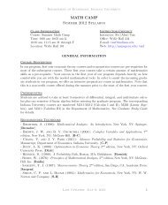
A portion of a sample of a configuration from P f is shown in Figure 1, where a square with<br />
upper left corner (i, j) is colored black iff η(i, j) = 1. These correspond to the horizontal<br />
edges of a uniform spanning tree in the square lattice. That is, if T is a spanning tree of<br />
Z 2 , then η(i, j) is the indicator that the edge from (i, j) to (i + 1, j) belongs to T . The<br />
portion of the spanning tree from which Figure 1 was constructed is shown in Figure 2.<br />
When T is chosen “uniformly” (see Pemantle (1991), Lyons (1998), or Benjamini, Lyons,<br />
Peres, and Schramm (2001) for definitions and information on this), then η has the law<br />
P f . This follows from the Transfer Current Theorem of Burton and Pemantle (1993) and<br />
the representation of the Green function as an integral; see Lyons with Peres (2003) for<br />
more details. Similarly, the edges of the uniform spanning forest (it is a tree only for d ≤ 4,<br />
as shown by Pemantle (1991)) parallel to the x1-axis in d dimensions correspond to the<br />
function<br />
f(x1, x2, . . . , xd) :=<br />
sin 2 πx1<br />
d<br />
j=1 sin2 πxj<br />
. (1.2)
§1. Introduction 4<br />
We remark that the uniform spanning tree is the so-called random-cluster model when one<br />
takes the limit q ↓ 0, then p ↓ 0, and finally the thermodynamic limit, the latter shown to<br />
exist by Pemantle (1991).<br />
Figure 1. A sample from P f of (1.1). Figure 2. A uniform spanning tree.<br />
Example 1.3. Let<br />
g(x) :=<br />
sin πx<br />
1 + sin 2 πx .<br />
Then the edges of the uniform spanning tree in the plane that lie on the x-axis have the<br />
law P g , as shown in Example 5.5 below.<br />
Example 1.4. Let<br />
f(x) := 1 | sin 2πx| − 1<br />
+<br />
2 2 cos 2πx .<br />
An elementary calculation shows that<br />
⎧<br />
1/2<br />
⎪⎨ 0<br />
f(k) =<br />
⎪⎩<br />
(−1)<br />
if k = 0,<br />
if k = 0 is even,<br />
(k−1)/2<br />
⎛<br />
⎝− 1<br />
(k−1)/2<br />
2 (−1)<br />
+<br />
2 π<br />
j<br />
⎞<br />
⎠ −<br />
2j + 1<br />
1<br />
πk<br />
if k is odd.<br />
j=0<br />
We shall show in Example 5.21 that the measure P f arises as follows. Given a spanning<br />
tree T of the square lattice, let η(n) be the indicator that en ∈ T , where en is the edge<br />
<br />
[(n/2, n/2), (n/2 + 1, n/2)] if n is even,<br />
en :=<br />
[((n + 1)/2, (n − 1)/2), ((n + 1)/2, (n + 1)/2)] if n is odd.
§1. Introduction 5<br />
The collection of edges {en ; n ∈ Z} is a zig-zag path in the plane. The law of η is P f when<br />
T is chosen as a uniform spanning tree. (Although it is not hard to see that the law of η<br />
is Z-invariant, by using planar duality, and although the law of η must be a determinantal<br />
probability measure because the law of T is, it is not apparent a priori that the law of η<br />
has the form P f for some f.)<br />
Example 1.5. Fix a horizontal edge of the hexagonal lattice (also known as the honeycomb<br />
lattice) and index all its vertical translates by Z. If one considers the standard measure<br />
of maximal entropy on perfect matchings of the hexagonal lattice, also called the dimer<br />
model and equivalent to lozenge tilings of the plane, and looks only at the edges indexed<br />
as above by Z, then the law is P f for f := 1 [1/3,2/3], as shown by Kenyon (1997).<br />
Example 1.6. It is interesting that the function f := 1 [0,1/2] for d = 1 also arises from a<br />
combinatorial model. In this case,<br />
⎧<br />
⎨ 1/2 if n = 0,<br />
f(n) = 0 if n = 0 is even,<br />
⎩<br />
1/(πin) if n is odd.<br />
The measure P f is the zig-zag process of Johansson (2002) derived from uniform domino<br />
tilings in the plane. For the definition of “uniform” in this case, see Burton and Pemantle<br />
(1993). A picture of a portion of such a tiling is shown in Figure 3. Consider the squares on<br />
a diagonal from upper left to lower right. The domino covering any such square also covers<br />
a second square. If this second square is above the diagonal, then we color the original<br />
square black, as shown in Figure 4. Johansson (2002) showed that the law of this process<br />
is P f when the diagonal squares are indexed by Z in the natural way. More generally,<br />
the processes P f for f the indicator of any arc of T are used by Borodin, Okounkov, and<br />
Olshanski (2000), Theorem 3, to describe the typical shape of Young diagrams.<br />
Example 1.7. Let 0 < a < 1 and d = 1. If f(x) := (1 − a) 2 /|e 2πix − a| 2 , then P f is a<br />
renewal process (Soshnikov, 2000). The number of 0s between successive 1s has the same<br />
distribution as the number of tails until 2 heads appear for a coin that has probability a<br />
of coming up tails. More explicitly, for n ≥ 1,<br />
Since<br />
P f [η(1) = · · · = η(n − 1) = 0, η(n) = 1 | η(0) = 1] = n(1 − a) 2 a n−1 . (1.3)<br />
f(x) =<br />
2πix<br />
1 − a ae<br />
+<br />
1 + a 1 − ae2πix 1<br />
1 − ae−2πix <br />
,
§1. Introduction 6<br />
Figure 3. A uniform domino tiling. Figure 4. A sample from P f of Example 1.6.<br />
expansion in a geometric series shows that<br />
f(k) =<br />
1 − a<br />
1 + a a|k| .<br />
We prove that P f is indeed this explicit renewal process after we prove Proposition 2.10,<br />
in which we extend this example to other regenerative processes.<br />
Example 1.8. If 0 < p < 1 and f : T d → [0, 1] is measurable, then a fair sample of P pf<br />
can be obtained from a fair sample of P f simply by independently changing each 1 to a 0<br />
with probability 1 − p.<br />
For general systems, note that the covariance of η(0) and η(k) for k ∈ Z d is −| f(k)| 2 .<br />
This is summable in k since f ∈ L 2 (T d ), but that is essentially the most one can say<br />
for its rate of decay. That is, given any 〈ak〉 ∈ ℓ 1 (Z d ), there is some (even continuous)<br />
f : T d → [0, 1] and some constant c > 0 such that | f(k)| 2 ≥ c|ak| for all k ∈ Z d , as shown<br />
by de Leeuw, Katznelson, and Kahane (1977). Observe also that as is the case for Gaussian<br />
processes, the processes studied here have the property that if the random variables are<br />
uncorrelated, then they are mutually independent.<br />
It is shown (in a much more general context) by Lyons (2002a) that these measures,<br />
as well as these measures conditioned on the values of η restricted to any finite subset of<br />
Z d , have the following negative association property: If A and B are increasing events that<br />
are measurable with respect to the values of η on disjoint subsets of Z d , then A and B are<br />
negatively correlated.
§1. Introduction 7<br />
In the order presented in this paper, our principal results are the following.<br />
• For all f, the process P f is a Bernoulli shift. This was shown by Shirai and Takahashi<br />
(2003) for those f such that <br />
n≥1 n| f(n)| 2 < ∞ by showing that those P f are weak<br />
Bernoulli.<br />
• For all f, the process P f stochastically dominates product measure P GM(f) and is<br />
stochastically dominated by product measure P 1−GM(1−f) , and these bounds are optimal.<br />
This is rather unexpected for the process of Example 1.2 related to the uniform spanning<br />
tree; explicit calculations are given below in Example 5.13 for this particular process. We<br />
give similar optimal bounds for full domination (uniform insertion and deletion tolerance)<br />
in terms of harmonic means.<br />
• We present methods to estimate the entropy of P f . For example, we show that<br />
for the function g in Example 1.3, the entropy of the system P g lies in the interval<br />
[0.69005, 0.69013]; see Example 6.15.<br />
• The process Pf is strong full K iff there is a nonzero trigonometric polynomial T<br />
|T |<br />
such that<br />
2<br />
f(1−f) ∈ L1 (Td ). This is equivalent to phase uniqueness in the sense that no<br />
conditioning at infinity can change the measure.<br />
• In one dimension, P f is strong K iff f(1 − f) has a positive geometric mean. This<br />
is equivalent to phase uniqueness when conditioning on one side only. Higher-dimensional<br />
versions of this will also be obtained.<br />
We shall give full definitions as they become needed. Some general background on<br />
determinantal probability measures is presented in Section 2, where we also exhibit a key<br />
representation of certain conditional probabilities as Szegő infima. The property of being a<br />
Bernoulli shift is proved in Section 3, while the auxiliary result that all P f have full support<br />
(except in two degenerate cases) is shown in Section 4. Properties concerning stochastic<br />
domination are proved in Section 5. These are used to estimate entropy in Section 6. More<br />
sophisticated methods of estimating entropy are also developed and illustrated in Section 6.<br />
The main result about phase multiplicity is proved in Section 7, while the one-sided case<br />
for d = 1 and its higher-dimensional generalizations are treated in Section 8. Finally, we<br />
end with some open questions in Section 9.<br />
The above definitions can be generalized to any countable abelian group with the<br />
discrete topology. For example, if we use Z × Z2, we obtain nontrivial joinings of the<br />
above systems with themselves. That is, suppose f : T → [0, 1] and h : T → [0, 1] are<br />
such that f ± h : T → [0, 1]. Then the function fh : T × {−1, 1} → [0, 1] defined by<br />
(x, ɛ) ↦→ f(x) + ɛh(x) gives a system that, when restricted to each copy of Z, is just P f ,<br />
but has correlations between the two copies that are given by h (the case h = 0 gives the
§2. Background 8<br />
independent joining). We can obtain slow decay of correlations between the two copies<br />
and negative associations in the joining itself; this is perhaps something that is not easy<br />
to construct directly.<br />
§2. Background.<br />
We first quickly review the probability measures studied in Lyons (2002a); see that<br />
paper for complete details.<br />
Let E be a finite or countable set and consider the complex Hilbert space ℓ 2 (E). Given<br />
any closed subspace H ⊆ ℓ 2 (E), let PH denote the orthogonal projection onto H. There<br />
is a unique probability measure P H on 2 E := {0, 1} E defined by<br />
P H [η(e1) = 1, . . . , η(ek) = 1] = det[(PHei, ej)]1≤i,j≤k<br />
(2.1)<br />
for all k ≥ 1 and any set of distinct e1, . . . , ek ∈ E; see, e.g., Lyons (2002a) or Daley and<br />
Vere-Jones (1988), Exercises 5.4.7–5.4.8. On the right-hand side, we are identifying each<br />
e ∈ E with the element of ℓ 2 (E) that is 1 in coordinate e and 0 elsewhere. In case H<br />
is finite-dimensional, then P H is concentrated on subsets of E of cardinality equal to the<br />
dimension of H.<br />
More generally, let Q be a positive contraction, meaning that Q is a self-adjoint<br />
operator on ℓ 2 (E) such that for all u ∈ ℓ 2 (E), we have 0 ≤ (Qu, u) ≤ (u, u). There is a<br />
unique probability measure P Q such that<br />
P Q [η(e1) = 1, . . . , η(ek) = 1] = det[(Qei, ej)]i,j≤k<br />
(2.2)<br />
for all k ≥ 1 and distinct e1, . . . , ek ∈ E. When Q is the orthogonal projection onto a<br />
closed subspace H, then P Q = P H . In fact, properties of P Q can be deduced from the<br />
special case of orthogonal projections. Since this will be useful for our analysis, we review<br />
this reduction procedure.<br />
Note first that uniqueness follows from the fact that (2.2) determines all finite-dimen-<br />
sional marginals via the inclusion-exclusion theorem. Indeed, we have the following formula<br />
for any disjoint pair of finite sets A, B ⊆ E (see, e.g., Lyons (2002a)):<br />
P Q 1B(e)e [η↾A ≡ 1, η↾B ≡ 0] = det + (−1) 1B(e) ′<br />
Qe, e <br />
e,e ′ ∈A∪B<br />
. (2.3)<br />
To show existence, let PH be any orthogonal projection that is a dilation of Q, i.e., H is a<br />
closed subspace of ℓ 2 (E ′ ) for some E ′ ⊇ E and for all u ∈ ℓ 2 (E), we have Qu = P ℓ 2 (E)PHu,<br />
where we regard ℓ 2 (E ′ ) = ℓ 2 (E)⊕ℓ 2 (E ′ \E). (In this case, Q is also called the compression
§2. Background 9<br />
of PH to ℓ 2 (E).) The existence of a dilation is standard and is easily constructed; see, e.g.,<br />
Lyons (2002a). Having chosen a dilation, we simply define P Q as the law of η restricted<br />
to E when η has the law P H . Then (2.2) is a special case of (2.1).<br />
A probability measure P on 2 E is said to have negative associations if for all pairs A<br />
and B of increasing events that are measurable with respect to the values of η on disjoint<br />
subsets of E, we have that A and B are negatively correlated with respect to P. The<br />
following conditional negative association (CNA) property is proved in Lyons (2002a)<br />
and a consequence of this (see Proposition 2.6) will be used frequently here.<br />
Theorem 2.1. If Q is any positive contraction on ℓ 2 (E), A is a finite subset of E, and<br />
η0 ∈ 2 A , then P Q [ · | η↾A = η0] has negative associations.<br />
We now assume that E = Z d . Then the group structure of Z d allows Z d to act<br />
naturally on ℓ2 (Zd ) and on 2Zd. The proof of the following lemma is straightforward and<br />
therefore skipped.<br />
Lemma 2.2. If Q is a Z d -invariant positive contraction on ℓ 2 (Z d ), then P Q is also Z d -<br />
invariant.<br />
As is well known, there exists a complex Hilbert-space isomorphism between L 2 (T d , λd)<br />
and ℓ 2 (Z d ) where T d is the d-dimensional torus R d /Z d and λd is unit Lebesgue measure on<br />
T d . This isomorphism is given by the Fourier transform f ↦→ f, where for f ∈ L 2 (T d , λd),<br />
we have f(k) = <br />
T d f(x)e −2πik·x dλd(x) for k ∈ Z d . If ek denotes the function x ↦→ e 2πik·x ,<br />
then the isomorphism takes the set {ek ; k ∈ Z d } to the standard basis for ℓ 2 (Z d ). From<br />
now on, we shall abbreviate L 2 (T d , λd) by L 2 (T d ).<br />
The following is well known.<br />
Theorem 2.3.<br />
(i) Let A ⊆ T d be measurable and consider the operator TA : L 2 (T d ) → L 2 (T d ) given by<br />
TA(g) = g1A .<br />
Then these projections (as A varies over the measurable subsets of T d ) correspond<br />
(via the Fourier isomorphism) to the Z d -invariant projections on ℓ 2 (Z d ).<br />
(ii) More generally, let f : T d → [0, 1] be measurable and consider the operator Mf :<br />
L 2 (T d ) → L 2 (T d ) given by<br />
Mf (g) = fg .<br />
Then these positive contractions (as f varies over the measurable functions from<br />
T d to [0, 1]) correspond (via the Fourier isomorphism) to the Z d -invariant positive<br />
contractions on ℓ 2 (Z d ). More specifically, Mf corresponds to convolution with f.
§2. Background 10<br />
As in the above theorem, an f : T d → [0, 1] yields a Z d -invariant positive contraction<br />
Qf on ℓ 2 (Z d ), which in turn yields a translation-invariant probability measure P Qf on 2 Z d<br />
that we denote more simply by P f .<br />
Lemma 2.4. Given f : T d → [0, 1] measurable and e1, . . . , ek ∈ Z d ,<br />
P f [η(e1) = 1, . . . , η(ek) = 1] = det[ f(ej − ei)]1≤i,j≤k .<br />
Proof. By definition, the left-hand side is det[(Qf ei, ej)]1≤i,j≤k. By Theorem 2.3(ii),<br />
(Qf ei, ej) = Mf eei, eej<br />
= f(ej − ei) .<br />
Remark 2.5. Lemma 2.4 says that for d = 1, the probability of having 1s on some finite<br />
collection of elements of Z is a particular minor of the Toeplitz matrix associated to f.<br />
Equation (2.3) shows a symmetry of P f and P 1−f , namely, if η has the distribution<br />
P f , then 1−η has the distribution P 1−f . Shirai and Takahashi (2003) prove the existence<br />
of P f by a different method and also note this symmetry.<br />
Although the last lemma gives us a formula for P f directly in terms of f without<br />
reference to any projections, it is still useful to know a specific projection of which Mf is<br />
a compression. Let f : T d → [0, 1] be measurable. Identifying T d+1 with T d × [0, 1), we let<br />
Af ⊆ T d+1 be the set {(x, y) ∈ T d+1 ; y ≤ f(x)}. Consider the projection TAf of L2 (T d+1 )<br />
given in Theorem 2.3(i). We view L 2 (T d ) as a subspace of L 2 (T d+1 ) by identifying g ∈<br />
L2 (Td ) with g ⊗ 1 ∈ L2 (Td+1 ), where (g ⊗ 1)(x, y) := g(x) for x ∈ Td , y ∈ T. The<br />
orthogonal projection P of L2 (Td+1 ) onto L2 (Td ) is then given by g ↦→ (x ↦→ <br />
g(x, y) dy).<br />
T<br />
A very simple calculation, left to the reader, shows that Mf is a compression of TAf ; i.e.,<br />
Mf = P TAf<br />
on L 2 (T d ) viewed as a subspace of L 2 (T d+1 ). For later use, let<br />
be the image of TAf .<br />
Hf := {g ∈ L 2 (T d+1 ) ; g = 0 a.e. on (Af ) c }<br />
(2.4)<br />
We next remind the reader of the notion of stochastic domination between two prob-<br />
ability measures on 2 E . First, if η, δ are elements of 2 E , we write η δ if η(e) ≤ δ(e) for<br />
all e ∈ E. A subset A of 2 E is called increasing if η ∈ A and η δ imply that δ ∈ A. If ν<br />
and µ are two probability measures on 2 E , we write ν µ if ν(A) ≤ µ(A) for all increasing<br />
sets A. A theorem of Strassen (1965) says that this is equivalent to the existence of a
§2. Background 11<br />
probability measure m on 2 E × 2 E that has ν and µ as its first and second marginals (i.e.,<br />
m is a coupling of ν and µ) and such that m is concentrated on the set {(η, δ) : η δ}<br />
(i.e., m is monotone).<br />
Throughout the paper, we shall use the following consequence of conditional negative<br />
association (Theorem 2.1), sometimes called joint negative regression dependence<br />
(see Pemantle (2000)).<br />
Proposition 2.6. Assume that {Xi}i∈I has conditional negative association, I is the dis-<br />
joint union of I1 and I2, and a, b ∈ {0, 1} I1 with ai ≤ bi for each i ∈ I1. Then<br />
[{Xi}i∈I2 | Xi = bi, i ∈ I1] [{Xi}i∈I2 | Xi = ai, i ∈ I1] ,<br />
where [Y | A] stands for the law of Y conditional on A.<br />
Lemma 2.7. Let f1, f2 : T d → [0, 1] with f1 ≤ f2 a.e. Then P f1 P f2 .<br />
Proof. This follows from a more general result (see Lyons (2002a)) that says that if Q1<br />
and Q2 are two commuting positive contractions on ℓ 2 (E) such that Q1 ≤ Q2 in the sense<br />
that Q2 − Q1 is positive, then P Q1 P Q2 . However, here is a more concrete proof in our<br />
case. Since f1 ≤ f2 a.e., it follows that Hf1 ⊆ Hf2, which implies by Theorem 6.2 in Lyons<br />
(2002a) that the projection measures P Hf 1 and P Hf 2 on Z d+1 satisfy P Hf 1 P Hf 2 and<br />
hence their restrictions to Z d satisfy the same relationship; i.e., P f1 P f2 .<br />
We close this section with a key representation of certain conditional probabilities and<br />
an application. The minimum in (2.5) below is often referred to as a Szegő infimum. For<br />
an infinite set B ⊆ Z d \ {0}, write<br />
P f [η(0) = 1 | η↾B ≡ 1] := lim<br />
n→∞ Pf [η(0) = 1 | η↾Bn ≡ 1] ,<br />
where Bn is any increasing sequence of finite subsets of B whose union is B. This is a<br />
decreasing limit by virtue of Proposition 2.6. Let (·, ·)f denote the usual inner product in<br />
the complex Hilbert space L 2 (f). For any set B ⊂ Z d , write [B]f for the closure in L 2 (f)<br />
of the linear span of the complex exponentials {ek ; k ∈ B}.<br />
Theorem 2.8. Let f : Td → [0, 1] be measurable and B ⊂ Zd with 0 /∈ B. Then<br />
P f <br />
[η(0) = 1 | η↾B ≡ 1] = min |1 − u| 2 <br />
f dλd ; u ∈ [B]f . (2.5)<br />
Proof. It suffices to prove the theorem for B finite since the infinite case then follows by a<br />
simple limiting argument. So assume that B is finite. Note that f(k − j) = (ej, ek)f , so<br />
that<br />
P f [η↾B ≡ 1] = det[(ej, ek)f ]j,k∈B ,
§2. Background 12<br />
and similarly for P f [η↾(B ∪ {0}) ≡ 1]. Thus, the left-hand side of (2.5) is a quotient<br />
of determinants. The fact that such a quotient has the form of the right-hand side is<br />
sometimes called Gram’s formula. We include the proof for the convenience of the reader.<br />
Since e0 = 1, it follows by row operations on the matrix [(ej, ek)] j,k∈B∪{0} that<br />
P f [η(0) = 1 | η↾B ≡ 1] = P ⊥<br />
[B]f 12 f , (2.6)<br />
where P ⊥<br />
[B]f denotes orthogonal projection onto the orthogonal complement of [B]f in<br />
L 2 (f). Since this is the squared distance from 1 to [B]f , the equation (2.5) now follows.<br />
An extension of the above reasoning, given in Lyons (2002a), provides the entire<br />
conditional probability measure:<br />
Theorem 2.9. Let f : T d → [0, 1] be measurable and B ⊂ Z d . Then the law of η↾(Z d \ B)<br />
conditioned on η↾B ≡ 1 is the determinantal probability measure corresponding to the<br />
positive contraction on ℓ 2 (Z d \ B) whose (j, k)-matrix entry is<br />
for j, k /∈ B.<br />
⊥<br />
P[B]f ej, P ⊥<br />
[B]f ek<br />
<br />
f .<br />
The Szegő infimum that appears in Theorem 2.8 involves trigonometric approximation,<br />
a classical area that has strong connections to the topics of prediction and interpolation<br />
for wide-sense stationary processes. We briefly discuss these topics now. In later sections,<br />
we describe more explicit connections to our results. Recall that a mean-0 wide-sense<br />
stationary process is a (not necessarily stationary) process 〈Yn〉 n∈Z d for which all the<br />
variables have finite variance and mean 0, and such that for each k ∈ Z d , the covariance<br />
Cov(Yn+k, Yn) = E[Yn+kYn] does not depend on n. There is then a positive measure G<br />
(called the spectral measure) on T d satisfying<br />
G(k) = Cov(Yn+k, Yn)<br />
for n, k ∈ Z d . It turns out that for a one-dimensional wide-sense stationary process, if<br />
G is absolutely continuous with density g, then GM(g) = 0 iff perfect linear prediction is<br />
possible, which means that Y0 is in the closed linear span of {Yn}n≤−1 in L 2 (Ω), where<br />
Ω is the underlying probability space. This was proved in various versions by Szegő,<br />
Kolmogorov and Kreĭn. Since the covariance with respect to P f of η(0) and η(k) for<br />
k ∈ Z d is also given by a Fourier coefficient (namely −| f(k)| 2 for k = 0) and since, as we<br />
shall see, the geometric mean of f will play an important role in classifying the behavior of
§2. Background 13<br />
P f as well, one might wonder about the relationship between our determinantal processes<br />
and wide-sense stationary processes. It is not hard to show that P f (viewed as a wide-sense<br />
stationary process) has a spectral measure G that is absolutely continuous with density g<br />
given by the formula<br />
g := f(0)1 − f ∗ f ,<br />
where ∗ denotes convolution and f(t) := f(1 − t). Other than the trivial cases f = 0<br />
and f = 1, it is easy to check that g is bounded away from 0 and so, in particular, its<br />
geometric mean is always strictly positive. This suggests that our results are perhaps not so<br />
connected to prediction and interpolation. However, it turns out that some of the questions<br />
that we deal with here (such as phase multiplicity and domination) concerning P f do have<br />
interpretations in terms of prediction and interpolation for wide-sense stationary processes<br />
whose spectral density is f (which does not include P f ). More specifics will be given in<br />
the relevant sections.<br />
Special attention is often devoted to stationary Gaussian processes, one reason being<br />
that their distribution is determined entirely by their spectral measure. It is known that a<br />
stationary Gaussian process with no deterministic component is a multistep Markov chain<br />
iff its spectral density is the reciprocal of a trigonometric polynomial; see Doob (1944).<br />
The analogous property for determinantal processes is regeneration:<br />
Proposition 2.10. If d = 1, then f is the reciprocal of a trigonometric polynomial of<br />
degree at most n iff P f is a regenerative process that regenerates after n successive 1s<br />
appear.<br />
This last property means that for any k, given that η↾[k + 1, k + n] ≡ 1, the future,<br />
η↾[k + n + 1, ∞), is conditionally independent of the past, η↾(−∞, k].<br />
Proof. Note first that because of Theorem 2.9, this regenerative property holds for P f iff<br />
for all j ≥ 0 and all C ⊂ (−∞, −n−1], we have P ⊥<br />
[B]f ej = P ⊥<br />
[B∪C]f ej, where B := [−n, −1].<br />
(Here, we are relying on the fact that P ⊥<br />
[B]f ejf > P ⊥<br />
[B∪C]f ejf if the vectors are not<br />
equal.) This is the same as P ⊥<br />
[B]f ej ⊥ [C]f for all j ≥ 0, or, in other words, there<br />
exists some uj ∈ [B]f with ej − uj ⊥ [B ∪ C]f . As this would have to hold for all C<br />
(and uj is independent of C), it is the same as the existence of some uj ∈ [B]f such<br />
that Tj := (ej − uj)f is analytic, i.e., Tj(k) = 0 for all k < 0. Now this implies that<br />
T0 = (1 − u0)f, whence T0(1 − u0) = T0(1 − u0). The left side of this last equation is<br />
an analytic function, while the right side is the conjugate of an analytic function (i.e., its<br />
Fourier coefficients vanish on Z + ). Therefore, both equal some constant, c. Hence<br />
f = T0<br />
1 − u0<br />
=<br />
c<br />
(1 − u0)(1 − u0) =<br />
c<br />
,<br />
|1 − u0| 2
§2. Background 14<br />
which is indeed the reciprocal of a trigonometric polynomial of degree at most n.<br />
Conversely, if 1/f is the reciprocal of a trigonometric polynomial of degree at most<br />
n, then since f ≥ 0, the theorem of Fejér and Riesz (see Grenander and Szegő (1984),<br />
p. 20) allows us to write f = c/|1 − u0| 2 for some conjugate-analytic polynomial u0 ∈ [B]f<br />
such that the analytic extension of 1 − u0 to the unit disc has no zeroes. We may rewrite<br />
this as (1 − u0)f = T0 for T0 := c/(1 − u0). Since T0 has an extension to the unit<br />
disc as the reciprocal of an analytic polynomial with no zeroes, it follows that T0 is also<br />
analytic. Multiplying both sides of this equation by e1 and rewriting e1u0f = c1(1−u ′ 1)f =<br />
c1(u0 − u ′ 1)f + c1T0 for some constant c1 and some u ′ 1 ∈ [B]f , we see that (e1 − u1)f = T1<br />
for u1 := c1(u0 − u ′ 1) ∈ [B]f and T1 := e1T0 + c1T0, an analytic function. Similarly,<br />
we may establish by induction that for each j ≥ 0, there is some uj ∈ [B]f such that<br />
Tj := (ej − uj)f is analytic. This proves the equivalence desired.<br />
We now use this proof to establish the explicit probabilistic form of the renewal process<br />
in Example 1.7. In this case, B = {−1} and one easily verifies that uj = a j+1 e−1, as is<br />
standard in the theory of linear prediction. Therefore,<br />
P f [η(j) = 1 | η(−1) = 1] = P ⊥<br />
[B]f ej 2 f = ej − uj 2 f = ej 2 f − uj 2 f =<br />
1 − a<br />
1 + a (1 − a2j+2 ) .<br />
It now suffices to verify that this is also true for the explicit renewal process described in<br />
Example 1.7. First, it is well known from basic renewal theory that for a renewal process,<br />
the probabilities P f [η(j) = 1 | η(−1) = 1] determine the distribution of the number of<br />
0s between two 1s. Hence to verify the above statement, one simply needs to check that<br />
these latter probabilities are related to the interrenewal distribution via the appropriate<br />
convolution-type equation. In this case, it comes down to verifying that for all j ≥ 0,<br />
1 − a<br />
1 + a (1 − a2j+2 ) = (j + 1)(1 − a) 2 a j 1 − a<br />
+<br />
1 + a<br />
This identity is easy to check.<br />
j<br />
k=1<br />
k(1 − a) 2 a k−1 (1 − a 2(j−k)+2 ) .
§3. The Bernoulli Shift Property 15<br />
§3. The Bernoulli Shift Property.<br />
In this section, we prove that the stationary determinantal processes studied here are<br />
Bernoulli shifts. We assume the reader is familiar with the basic notions of a Bernoulli<br />
shift (see, e.g., Ornstein (1974)).<br />
Theorem 3.1. Let f : T d → [0, 1] be measurable. Then P f is a Bernoulli shift; i.e., it is<br />
isomorphic (in the sense of ergodic theory) to an i.i.d. process.<br />
Before beginning the proof, we present a few preliminaries. We first recall the defini-<br />
tion of the d-metric.<br />
Definition 3.2. If µ and ν are Zd-invariant probability measures on 2Zd, then<br />
(η, Z<br />
d(µ, ν) := inf m δ) ∈ 2<br />
m d<br />
× 2 Zd<br />
; η(0) = δ(0) <br />
,<br />
where the infimum is taken over all couplings m of µ and ν that are Z d -invariant.<br />
The following is a slight generalization of a well-known result (see, for example, page 75<br />
in Liggett (1985)). The proof is an immediate consequence of the existence of a monotone<br />
coupling and is left to the reader.<br />
Lemma 3.3. Suppose that σ1, σ2, ν and µ are Z d -invariant probability measures on 2 Zd<br />
such that ν σi µ for both i = 1, 2. Then<br />
d(σ1, σ2) ≤ µ[η(0) = 1] − ν[η(0) = 1] .<br />
Proposition 3.4. Let f, g : T d → [0, 1] be measurable. Then<br />
d(P f , P g ) ≤<br />
<br />
T d<br />
|f − g| dλd .<br />
Proof. Because of Lemma 2.7, we may apply Lemma 3.3 to σ1 := P f , σ2 := P g , ν := P f∧g ,<br />
and µ := P f∨g . We obtain that<br />
d(P f , P g ) ≤<br />
<br />
T d<br />
<br />
f ∨ g dλd −<br />
T d<br />
<br />
f ∧ g dλd =<br />
T d<br />
|f − g| dλd .<br />
Proof of Theorem 3.1. The first step is to approximate f by trigonometric polynomials.<br />
Let Kr be the rth Fejér kernel for T,<br />
Kr := <br />
|j|≤r<br />
<br />
1 − |j|<br />
<br />
ej ,<br />
r + 1
§3. The Bernoulli Shift Property 16<br />
and define K d r (x1, . . . , xd) := d<br />
i=1 Kr(xi). It is well known that K d r is a positive summability<br />
kernel, so that if we define gr by<br />
gr := f ∗ K d r ,<br />
then 0 ≤ gr ≤ 1 and limr→∞ gr = f a.e. and in L 1 (T d ).<br />
Next, since each K d r is a trigonometric polynomial, so is each gr. From this and<br />
Lemma 2.4, it is easy to see that there is a constant C such that P gr (A∩B) = P gr (A)P gr (B)<br />
if A is of the form η ≡ 1 on S1 and B is of the form η ≡ 1 on S2 with S1 and S2 being<br />
finite sets and having distance at least C between them. From this, a standard argument in<br />
probability (a π-λ argument) shows that if A is any event depending only on locations S1<br />
and if B is any event depending only on locations S2 with S1 and S2 possibly infinite sets<br />
having distance at least C between them, then P gr (A ∩ B) = P gr (A)P gr (B). A process<br />
with this property is called a finitely dependent process and this property implies it is<br />
a Bernoulli shift (e.g., the so-called very weak Bernoulli condition is immediately verified;<br />
see Ornstein (1974) for this definition for d = 1 and, e.g., Steif (1991) for general d).<br />
Since the processes that are Bernoulli shifts are closed in the d metric (see Ornstein<br />
(1974)) and Proposition 3.4 tells us that limr→∞ d(P gr , P f ) = 0, we conclude that P f is<br />
a Bernoulli shift.<br />
Remark 3.5. An important property of 1-dimensional stationary processes is the weak<br />
Bernoulli (WB) property. This is also referred to as “β-mixing” and “absolute regularity”<br />
in the literature. Despite its name, it is known that WB is strictly stronger than Bernoul-<br />
licity. It is easy to check that “aperiodic” regenerative processes and finitely dependent<br />
processes are WB. Hence, by our earlier results, if f is a trigonometric polynomial or the<br />
inverse of a trigonometric polynomial (or if 1 − f is the inverse of a trigonometric polyno-<br />
mial), then P f is WB. This is subsumed by the independent work of Shirai and Takahashi<br />
(2003), who showed that P f is WB whenever <br />
n≥1 n| f(n)| 2 < ∞. The precise class of f<br />
for which P f is WB is not known. We also note that it follows from Smorodinsky (1992)<br />
that if f is a trigonometric polynomial, then P f is finitarily isomorphic to an i.i.d. process.
§4. Support of the Measures 17<br />
§4. Support of the Measures.<br />
In this section, we show that all of the probability measures P f have full support<br />
except in two degenerate cases. We begin with the following lemma.<br />
Lemma 4.1. Let H be a closed subspace of ℓ 2 (E) and let A and B be finite disjoint subsets<br />
of E. Then<br />
P H [η(e) = 1 for e ∈ A, η(e) = 0 for e ∈ B] > 0<br />
if and only if {PH(e)}e∈A ∪ {P H ⊥(e)}e∈B is linearly independent.<br />
Proof. In the special case that A or B is empty, the result follows from Lyons (2002a). In<br />
general, {PH(e)}e∈A ∪ {P H ⊥(e)}e∈B is linearly independent if and only if {PH(e)}e∈A and<br />
{P H ⊥(e)}e∈B are each linearly independent sets. Also, P H [η↾A ≡ 1, η↾B ≡ 0] > 0 if and<br />
only if P H [η↾A ≡ 1] > 0 and P H [η↾B ≡ 0] > 0 since<br />
P H [η↾A ≡ 1, η↾B ≡ 0] ≥ P H [η↾A ≡ 1]P H [η↾B ≡ 0]<br />
by the negative association property, Theorem 2.1. Thus, the general case follows from<br />
the special case.<br />
Theorem 4.2. P f has full support for any function f : T d → [0, 1] other than 0 or 1.<br />
Proof. Since marginals of probability measures with full support clearly have full support,<br />
it suffices to prove the result for P H when H is a closed Z d -invariant subspace of ℓ 2 (Z d )<br />
other than ℓ 2 (Z d ) or 0. If we translate over to L 2 (T d ), we see, by Lemma 4.1, that it<br />
suffices to show that if A ⊆ T d with 0 < λd(A) < 1 and n1, . . . , nk, m1, . . . , mℓ are all<br />
distinct elements of Z d , then<br />
{enj 1A}1≤j≤k ∪ {emr1A c}1≤r≤ℓ<br />
is linearly independent. Suppose that c1, . . . , ck, d1, . . . , dℓ are complex numbers such that<br />
k<br />
j=1<br />
cjenj 1A +<br />
ℓ<br />
r=1<br />
dremr1A c = 0 .<br />
From this it follows that k<br />
j=1 cjenj = 0 a.e. on A. Since λd(A) > 0, we have that<br />
k<br />
j=1 cjenj is 0 on a set of positive measure. It is well known that this implies that<br />
c1, . . . , ck vanish (the proof uses induction on d and Fubini’s theorem). Similarly, d1, . . . , dℓ<br />
vanish.
§5. Domination Properties 18<br />
§5. Domination Properties.<br />
In this section, we study the question of which product measures are stochastically<br />
dominated by P f and which product measures stochastically dominate P f . For simplicity,<br />
we give our first results for d = 1, and only afterwards describe how these results extend<br />
to higher dimensions. We also treat a different notion of “full domination” at the end of<br />
the section. Recall that for f : T d → [0, 1], we define<br />
<br />
GM(f) := exp<br />
Td log f dλd .<br />
We introduce an auxiliary stronger notion of domination than , but only in the case<br />
where one of the measures is a product measure. Let µp denote product measure with<br />
density p.<br />
Definition 5.1. A stationary process {ηn}n∈Z with distribution ν strongly dominates<br />
µp, written µp s ν, if for any n and any a1, . . . , an ∈ {0, 1},<br />
P[η0 = 1 | ηi = ai, i = 1, . . . , n] ≥ p .<br />
Similarly, we define ν s µp if the above inequality holds when ≥ is replaced by ≤.<br />
lemma.<br />
The following lemma is easy and well known; it is sometimes referred to as Holley’s<br />
Lemma 5.2. If µp s ν, then µp ν.<br />
The converse is not true, as we shall see later (Remark 6.4). In light of Lemma 2.7,<br />
we have that if p ≤ f ≤ q, then<br />
µp P f µq .<br />
The optimal improvement of these stochastic bounds is as follows.<br />
Theorem 5.3. For any f : T → [0, 1], we have µp P f iff p ≤ GM(f) iff µp s P f .<br />
Similarly, P f µq iff q ≥ 1 − GM(1 − f) iff P f s µq. In addition, for any stationary<br />
process µ that has conditional negative association, we have µp µ iff µp s µ.<br />
Proof. Let dn := Dn−1(f) be the probability of having n 1s in a row. According to Szegő’s<br />
theorem (Grenander and Szegő (1984), pp. 44, 66), dn+1/dn is decreasing in n and<br />
In particular, dn+1/dn ≥ GM(f) for all n.<br />
lim<br />
n→∞ dn+1/dn = GM(f) = lim<br />
n→∞ d1/n n .
§5. Domination Properties 19<br />
Proposition 2.6 implies that for any fixed n,<br />
P f [η0 = 1 | ηi = ai, i = 1, . . . , n]<br />
is minimized among all a1, . . . , an ∈ {0, 1} when a1 = a2 = · · · = an = 1. In this case,<br />
the value is dn+1/dn. Since this is at least GM(f), we deduce that if p ≤ GM(f), then<br />
µp s P f and hence that µp P f .<br />
Conversely, if µp P f , then certainly p n ≤ dn for all n. Hence p ≤ GM(f). The<br />
second to last statement can be proved in the same way or can be concluded by symmetry.<br />
Finally, the last statement can be proved in a similar fashion.<br />
Remark 5.4. The above theorem gives us two interesting examples. First, if we take<br />
f := 1A where A has Lebesgue measure 1 − ɛ, then d(P f , δ1) ≤ ɛ by Proposition 3.4,<br />
but nonetheless, P f does not dominate any nontrivial product measure since GM(f) = 0.<br />
Second, if we take f := 1 [0,1/2] + .4 · 1 [1/2,1], then f < 1/2 on a set of positive measure,<br />
but nonetheless P f dominates P 1/2 = µ 1/2 since GM(f) = (.4) 1/2 > 1/2.<br />
Example 5.5. Let f be as in Example 1.2, so that P f is the law of the horizontal edges<br />
of the uniform spanning tree in the plane. In order to examine a 1-dimensional process,<br />
let us consider only the edges lying on the x-axis. If we let<br />
<br />
g(x) := f(x, y) dλ1(y) ,<br />
T<br />
then the edges lying on the x-axis have the law P g since g(k) = f(k, 0) for all k ∈ Z. Since<br />
an antiderivative of 1/(1 + a sin 2 πy) is<br />
we have<br />
arctan √ 1 + a tan πy <br />
g(x) =<br />
π √ 1 + a<br />
sin πx<br />
1 + sin 2 πx ,<br />
as given in Example 1.3. We claim that P g strongly dominates µp for p := √ 2 − 1,<br />
and this is optimal. In order to show this, we calculate GM(g). Write g1(x) := sin 2 πx.<br />
Then (GM(g)) 2 = GM(g1)/GM(1 + g1). Let G1 be the harmonic extension of log g1 from<br />
the circle to the unit disc. Then log g1 dλ1 = G1(0) by the mean value property of<br />
harmonic functions. Since g1 = |(1 − e1)/2| 2 , we see that G1 is the real part of the<br />
analytic function z ↦→ 2 log[(1 − z)/2] in the unit disc, from which we conclude that<br />
G1(0) = log(1/4). Therefore, GM(g1) = 1/4. Similarly, 1+g1 = |[ √ 2+1−( √ 2−1)e1]/2| 2 ,<br />
,
§5. Domination Properties 20<br />
whence GM(1 + g1) = [( √ 2 + 1)/2] 2 . Therefore GM(g) = √ 2 − 1 = 0.4142 + , as desired. It<br />
turns out that q := 1 − GM(1 − g) = 1 − 2( √ 2 − 1)e −2G/π = 0.5376 + , where<br />
G :=<br />
∞<br />
k=0<br />
(−1) k<br />
= 0.9160−<br />
(2k + 1) 2<br />
is Catalan’s constant. Thus, P g s µq. It is interesting how close p and q are.<br />
(5.1)<br />
We now introduce some new mixing conditions. Given a positive integer r, we may<br />
restrict P f to 2 rZ . If we identify rZ with Z, then we obtain the process P fr , where<br />
fr(t) := 1<br />
r<br />
<br />
x∈r −1 t<br />
f(x) ,<br />
where r −1 t := {x ∈ T ; rx = t}. The reason that this restriction is equal to P fr is that<br />
for all k ∈ Z, we have fr(k) = f(rk), as is easy to check. Because of this relation, we<br />
have that |fr(t) − f(0)| 2 dλ1(t) → 0 as r → ∞, so that by Lemma 3.3, it follows that<br />
d(P fr , P f(0) ) → 0 as r → ∞. (It is not hard to show that a similar property holds for any<br />
Kolmogorov automorphism (see Definition 7.1), while the example in Remark 6.4 shows<br />
that this property can occur in other cases as well.) In fact, we often have a stronger<br />
convergence for our determinantal processes, as we show next.<br />
Theorem 5.6. Let f : T → [0, 1] be measurable. If GM(f) > 0 or f is bounded away<br />
from 0 on an interval of positive length, then there exist constants pr → f(0) such that<br />
P fr P pr for all r. Therefore, if GM f(1 − f) > 0 or if f is continuous and not equal<br />
to 0 nor 1, then there exist constants pr, qr → f(0) such that P pr P fr P qr for all r.<br />
Of course, in view of Theorem 5.3, we use pr := GM(fr) and qr := 1 − GM(1 − fr).<br />
Thus, the theorem is an immediate consequence of the following lemma.<br />
Lemma 5.7. Let f : T → [0, 1] be measurable. If GM(f) > 0 or f is bounded away from 0<br />
on an interval of positive length, then GM(fr) → f(0) as r → ∞.<br />
Proof. We have seen that fr → f(0) · 1 in L 2 , whence also in measure. Therefore log fr →<br />
(log f(0)) · 1 in measure. Thus, it remains to show that {log fr} is uniformly integrable (at<br />
least, for all large r). Suppose first that GM(f) > 0.<br />
Given h ∈ L 1 (T), write h (r) (t) := h(rt), so that h (r) (k) is 0 when k is not a multiple<br />
of r and is h(k/r) when k is a multiple of r. For any g, h ∈ L2 (T), we have<br />
<br />
gr(t)h(t) dλ1(t) = <br />
gr(k) h(k) = <br />
g(rk) h(k) = <br />
g(k) h (r) (k)<br />
T<br />
k∈Z<br />
T<br />
k∈Z<br />
T<br />
k∈Z<br />
<br />
= g(t)h (r) <br />
(t) dλ1(t) = g(t)h(rt) dλ1(t) . (5.2)
§5. Domination Properties 21<br />
Therefore, for any set A ⊆ T, we have<br />
<br />
A<br />
<br />
log(fr) dλ1 ≥<br />
A<br />
<br />
(log f)r dλ1 =<br />
r −1 A<br />
log f dλ1 ;<br />
the inequality follows by concavity of log, while the equality follows from (5.2) applied to<br />
g := log f and h := 1A. Given any ɛ ∈ 0, f(0) , let A r ɛ := {t ; fr(t) < ɛ}. Note that for<br />
any measurable A ⊂ T, we have λ1(r −1 A) = λ1(A). Since fr → f(0) · 1 in measure, it<br />
follows that<br />
Since log f is integrable, it follows that<br />
lim<br />
r→∞ λ1(r −1 A r ɛ) = lim<br />
r→∞ λ1(A r ɛ) = 0 .<br />
<br />
lim<br />
r→∞<br />
r−1Ar log f dλ1 = 0 .<br />
ɛ<br />
This establishes the uniform integrability in the first case.<br />
In the second case where f ≥ c > 0 on an interval of length ɛ > 0, we have that<br />
fr ≥ cɛ on all of T for all r > 1/ɛ. It is then obvious that {log fr} is uniformly integrable<br />
for all r > 1/ɛ.<br />
Remark 5.8. There are functions f with f > 0 a.e., yet GM(fr) = 0 for all r. For example,<br />
enumerate the rationals {xj ; j ≥ 1} in (0, 1) and choose ɛj > 0 such that xj + ɛj < 1 and<br />
<br />
j ɛj < 1. Define An := [0, 1] \ <br />
j>n [xj, xj + ɛj] and f0(x) := e −1/x . Then one can show<br />
that<br />
is such an example.<br />
f(x) := f0(x)1A0(x) +<br />
∞<br />
f0(x − xn)1 [xn,xn+ɛn]∩An (x)<br />
n=1<br />
We turn next to the extension of the prior results to higher dimensions. This is<br />
basically straightforward, but has interesting applications, as we shall see. First, we recall<br />
the usual notion of the past σ-field Past(k) at a point k ∈ Z d . We use lexicographic<br />
ordering on Z d , i.e., write (k1, k2, . . . , kd) ≺ (l1, l2, . . . , ld) if ki < li when i is the smallest<br />
index such that ki = li. Then define Past(k) to be the σ-field generated by η(j) for all<br />
j ≺ k. More generally, the past σ-field could be defined with respect to any ordering of<br />
Z d , which means the selection of a set Π ⊂ Z d that has the properties Π∪(−Π) = Z d \{0},<br />
Π ∩ (−Π) = ∅, and Π + Π ⊂ Π. The associated ordering is that where k ≺ l iff l − k ∈ Π.<br />
PastΠ(u) will denote the past of u with respect to the ordering Π, i.e., {v ; v ≺ u}. Thus,<br />
PastΠ(0) is just −Π. (For a characterization of all orders, see Teh (1961), Zaĭceva (1953),<br />
or Trevisan (1953).) As before, let µp denote product measure with density p.
§5. Domination Properties 22<br />
Definition 5.9. Given an ordering Π, a stationary process {ηn} n∈Z d with distribution ν<br />
strongly dominates µp, written µp s ν, if<br />
P[η0 = 1 | PastΠ(0)] ≥ p ν-a.s.<br />
Similarly, we define ν s µp if the above inequality holds when ≥ is replaced by ≤. (Note<br />
that the ordering Π here is suppressed in the notation.)<br />
Although we have phrased it differently, in one dimension, this is equivalent to Defi-<br />
nition 5.1 when Π = {−1, −2, . . .}. Again, we have a version of Holley’s lemma:<br />
Lemma 5.10. Given any ordering Π, if µp s ν, then µp ν.<br />
(Note that to produce a monotone coupling for a general ordering with respect to a<br />
set Π, it is enough to do so for the measures restricted to any finite B ⊂ Z d . Given such a<br />
B, order B by the restriction of ≺ to B and couple the measures by adding sites from B<br />
in this order.)<br />
We now prove<br />
Theorem 5.11. Fix any ordering Π. For any measurable f : T d → [0, 1], we have µp P f<br />
iff p ≤ GM(f) iff µp s P f . Similarly, P f µq iff q ≥ 1 − GM(1 − f) iff P f s µq. In<br />
addition, for any stationary process µ that has conditional negative association, we have<br />
µp µ iff µp s µ.<br />
Proof. Proposition 2.6 and Theorem 2.8 imply that<br />
<br />
<br />
f<br />
ess inf P η(0) = 1 | PastΠ(0) = inf P f <br />
[η(0) = 1 | η↾A ≡ 1] ; A ⊂ −Π is finite<br />
= P f [η(0) = 1 | η↾(−Π) ≡ 1]<br />
<br />
= min |1 − T | 2 <br />
f dλd ; T ∈ [−Π]f .<br />
By Helson and Lowdenslager (1958), the latter quantity equals GM(f). Therefore, p ≤<br />
GM(f) iff µp s P f . On the other hand, if µp P f , then let A(r) be the finite subset of<br />
−Π consisting of all points within some large radius r about 0. Let a1 ≺ a2 ≺ · · · ≺ an be<br />
the elements of A(r) in order, where n := |A(r)|, and write Aj := A(r) ∩ (−Π + aj). Then<br />
n<br />
P f [η(aj) = 1 | η↾Aj ≡ 1] .<br />
p n ≤ P f [η↾A(r) ≡ 1] =<br />
j=1<br />
Most terms in this product are quite close to GM(f), while all lie in [GM(f), 1]. It follows<br />
that<br />
lim<br />
r→∞ Pf [η↾A(r) ≡ 1] 1/n = GM(f) ,<br />
so that p ≤ GM(f). Finally, the remaining statements can be proved in a similar fashion.
§5. Domination Properties 23<br />
Remark 5.12. It follows from Theorem 5.11 that the choice of ordering Π does not de-<br />
termine whether µp s P f . This is not true for general stationary processes, even in one<br />
dimension. We are grateful to Olle Häggström for the following simple example. Let µ be<br />
the distribution on {0, 1} 2 given by<br />
µ = (1/7)(δ (0,0) + δ (0,1)) + (2/7)δ (1,0) + (3/7)δ (1,1) .<br />
Let η ∈ {0, 1} Z be such that with probability 1/2, (η2n, η2n+1) are chosen independently<br />
each with distribution µ and otherwise (η2n−1, η2n) are chosen independently each with<br />
distribution µ. Let ν be the law of η. If Π := Z − , then µp s ν iff p ≤ 1/2, while if<br />
Π := Z + , then µp s ν iff p ≤ 4/7.<br />
Example 5.13. Let f be as in Example 1.2, so that P f is the law of the horizontal edges of<br />
a uniform spanning tree in the square lattice Z 2 . By Kasteleyn (1961) or Montroll (1964),<br />
we have <br />
T 2<br />
log 4(sin 2 πx + sin 2 πy) dλ2(x, y) = 4G<br />
π = 1.1662+ , (5.3)<br />
where G is again Catalan’s constant (5.1). As we have shown in Example 5.5, GM(sin 2 πx) =<br />
1/4, whence by (5.3), GM(f) = e −4G/π = GM(1 − f), where we are using the observation<br />
that 1 − f(x, y) = f(y, x). (This last identity has a combinatorial reason arising from<br />
planar dual trees.) Therefore µp P f µ1−p for p := e −4G/π = 0.3115 + and this p is<br />
optimal (on each side). This result in itself is rather surprising and it would be fascinating<br />
to see an explicit monotone coupling.<br />
For f : T d → [0, 1] measurable and r = (r1, r2, . . . , rd) ∈ Z d with all rj > 0, define<br />
fr(t) :=<br />
1<br />
d<br />
j=1 rj<br />
<br />
x∈r −1 t<br />
f(x) ,<br />
where r −1 (t1, t2, . . . , td) := {(x1, x2, . . . , xd) ∈ T d ; ∀j rjxj = tj}. Write r → ∞ to mean<br />
that min rj → ∞. The following is a straightforward extension of Theorem 5.6. We leave<br />
its proof to the reader.<br />
Theorem 5.14. Let f : T d → [0, 1] be measurable. If GM(f) > 0 or f is positive on a<br />
non-empty open set, then there exist constants pr → f(0) as r → ∞ such that P fr P pr<br />
for all r. Therefore, if GM f(1 − f) > 0 or if f is continuous and not equal to 0 nor 1,<br />
then there exist constants pr, qr → f(0) such that P pr P fr P qr for all r.<br />
Consider now a domination property even stronger than our previously defined strong<br />
domination. Let Z be the σ-field generated by η(k) for k = 0.
§5. Domination Properties 24<br />
Definition 5.15. A stationary process {ηn} n∈Z d with distribution ν fully dominates<br />
µp, written µp f ν, if<br />
P[η0 = 1 | Z] ≥ p ν-a.s.<br />
In this situation, we also say that ν is uniformly insertion tolerant at level p. Similarly,<br />
we define ν f µp if the above inequality holds when ≥ is replaced by ≤, and say that ν<br />
is uniformly deletion tolerant at level 1 − p. We say that ν is uniformly insertion<br />
tolerant if µp f ν for some p > 0 and that ν is uniformly deletion tolerant if ν f µp<br />
for some p < 1.<br />
We show that the optimal level of uniform insertion tolerance of a determinantal<br />
process P f is the harmonic mean of f, defined as<br />
<br />
HM(f) :=<br />
Note that HM(f) = 0 iff 1/f is not integrable.<br />
T d<br />
−1 dλd<br />
f<br />
Theorem 5.16. For any measurable f : T d → [0, 1], we have µp f P f iff p ≤ HM(f).<br />
Similarly, P f f µq iff q ≥ 1 − HM(1 − f).<br />
Proof. By Proposition 2.6 and Theorem 2.8, we have<br />
<br />
<br />
f<br />
ess inf P η(0) = 1 | Z = inf<br />
= P f <br />
[η(0) = 1 | η↾B ≡ 1] = min<br />
P f [η(0) = 1 | η↾A ≡ 1] ; A ⊂ Z d \ {0} is finite<br />
.<br />
<br />
|1 − T | 2 <br />
f dλd ; T ∈ [B]f ,<br />
where B := Z d \ {0}. As shown by Kolmogorov (1941a, 1941b) for d = 1, the latter equals<br />
HM(f). The proof extends immediately to general d. This proves the first assertion. The<br />
second follows by symmetry.<br />
Remark 5.17. Since a proof of Kolmogorov’s theorem that<br />
<br />
min<br />
|1 − T | 2 <br />
f dλd ; T ∈ [B]f = HM(f) ,<br />
where B := Z d \ {0}, is difficult to find in readily accessible sources, we provide one here.<br />
We have<br />
where<br />
<br />
min<br />
|1 − T | 2 f dλd ; T ∈ [B]f<br />
u := P ⊥<br />
[B]f 12 f .<br />
<br />
= u 2 f ,
§5. Domination Properties 25<br />
Now g ⊥ [B]f iff g ∈ L 2 (f) and gf(k) = 0 for all k ∈ B. The latter condition holds iff gf<br />
is a constant. If g = 0, then we deduce that 1/f ∈ L 2 (f), i.e., HM(f) > 0. Therefore,<br />
[B] ⊥ f =<br />
Hence u = 0 if HM(f) = 0, while otherwise,<br />
as desired.<br />
0 if HM(f) = 0,<br />
C/f if HM(f) > 0.<br />
u 2 f = |(1, HM(f)/f)f | 2 = HM(f) ,<br />
Remark 5.18. It is easy to find f such that GM(f) > 0 and HM(f) = 0. Indeed, a natural<br />
such example is the function g of Example 1.3. For any such f, the corresponding process<br />
P f strongly dominates a nontrivial product measure, but does not fully dominate any<br />
nontrivial product measure. In addition, for any function f such that HM(f) > 0 and f is<br />
not constant a.e., GM(f) > HM(f) (as a consequence of Jensen’s inequality), so that P f<br />
will strongly dominate strictly more product measures than it will fully dominate.<br />
Example 5.19. Let f be as in (1.2), so that P f is the law of the edges of the uniform<br />
spanning forest in Z d that lie parallel to the x1-axis. Then P f is uniformly deletion tolerant<br />
iff d ≥ 4. This is because 1/(1 − f) is integrable iff d ≥ 4. For example, when d = 4, we<br />
obtain full domination by µp with p := 0.66425 − , where we have calculated HM(1 − f) as<br />
follows. First, we have<br />
whence<br />
<br />
T4 1/(1 − f) dλ4 = 1 + 1<br />
<br />
2<br />
= 1 + 1<br />
<br />
2<br />
1/(1 − f) = 1 +<br />
T 3<br />
T 2<br />
1<br />
4<br />
j=2 sin2 πxj<br />
3<br />
sin 2 πx1<br />
4<br />
j=2 sin2 πxj<br />
j=2 sin2 πxj<br />
dλ3(x2, x3, x4)<br />
1<br />
,<br />
<br />
1 + 3<br />
j=2 sin2 πxj<br />
dλ2(x2, x3) .<br />
This last integral has no simple form and is calculated numerically. This gives the value<br />
reported for 1 − HM(1 − f). For large d, we have 1 − HM(1 − f) ∼ 1/d. Indeed, write λ ∗ d−1<br />
for Lebesgue measure on R d−1 . Letting<br />
<br />
Ad :=<br />
T d−1<br />
d − 1<br />
d<br />
j=2 2 sin2 πxj<br />
dλd−1(x2, . . . , xd) ,
§5. Domination Properties 26<br />
we have that<br />
(d − 1)(1 − HM(1 − f)) =<br />
Ad<br />
1 + Ad/(d − 1) .<br />
Hence it suffices to show that limd→∞ Ad = 1. To show this, note that<br />
∞<br />
Ad =<br />
0<br />
2<br />
≤<br />
0<br />
λd−1<br />
λd−1<br />
d <br />
j=2<br />
d <br />
10(d−1)<br />
+<br />
2<br />
∞<br />
+<br />
j=2<br />
2 sin 2 <br />
πxj < (d − 1)/t dt<br />
2 sin 2 <br />
πxj < (d − 1)/t dt<br />
λd−1<br />
λ<br />
10(d−1)<br />
∗ d−1<br />
d <br />
2<br />
→ 1 [0,1](t) dt = 1<br />
0<br />
j=2<br />
2 sin 2 <br />
πxj < (d − 1)/2 dt<br />
<br />
∀j |xj| < 1/2 and<br />
d<br />
j=2<br />
8x 2 <br />
j < (d − 1)/t dt<br />
as d → ∞, where we have used the weak law of large numbers and the bounded convergence<br />
theorem for the first piece, a standard large-deviation result for the second piece, and an<br />
easy estimate on the third piece. The reverse inequality obtains by using only the first piece.<br />
Thus, Ad → 1, as desired. This value of 1 − HM(1 − f), which gives a full domination<br />
upper bound on P f , should be compared to f(0) = 1/d (by symmetry), which is the<br />
probability of a 1 at a site. On the other hand, for no d is the process uniformly insertion<br />
tolerant since 1/f is never integrable. We remark that for the full uniform spanning forest<br />
measure on Z d (considering edges in all directions), we have change intolerance, meaning<br />
that P[η(0) = 1 | Z] ∈ {0, 1} a.s. This follows from a result of Benjamini, Lyons, Peres,<br />
and Schramm (2000), as explained by Heicklen and Lyons (2002).<br />
Example 5.20. Let g(x) be as in Example 1.3, so that the edges of the uniform spanning<br />
tree in the plane that lie on the x-axis have the law P g . We have P g f µp for p :=<br />
(1 + π)/(1 + 2π) = 0.56865 + , and this is optimal. This is because<br />
<br />
<br />
1/(1 − g) dλ =<br />
<br />
1 + sin<br />
T<br />
T<br />
2 <br />
πx + sin πx 1 + sin 2 <br />
πx dλ(x)<br />
<br />
= 3/2 +<br />
<br />
sin πx 1 + sin 2 πx dλ(x) .<br />
An antiderivative of this integrand is<br />
− 1<br />
π arctan<br />
<br />
<br />
cos πx<br />
<br />
2<br />
1 + sin πx<br />
T<br />
− 1 <br />
cos πx 1 + sin<br />
2π 2 πx ,
§5. Domination Properties 27<br />
whence the remaining integral is 1/2 + 1/π. Therefore <br />
T<br />
1/(1 − g) dλ = 2 + 1/π and<br />
1 − HM(1 − g) = (1 + π)/(1 + 2π), as desired. Observe that 1/g = ∞ and so the process<br />
is not uniformly insertion tolerant. Similarly, for the edges lying on the x-axis of the<br />
uniform spanning tree in 3 dimensions, we have full domination by µp with p := 0.37732 + .<br />
Here, the law of these edges is Ph , where<br />
<br />
<br />
h(x) := f(x, y, z) dλ2(y, z) =<br />
T 2<br />
T<br />
sin 2 πx<br />
sin 2 πx + sin 2 πy 1 + sin 2 πx + sin 2 πy dλ1(y) .<br />
This integral has no simpler form, so to compute p := 1 − HM(1 − h), we calculated<br />
h numerically and used the result to calculate the harmonic mean numerically. Since<br />
1/h = ∞, as is easily checked, this process is not uniformly insertion tolerant. Similarly,<br />
one can check that the process of edges lying on the x-axis of the uniform spanning tree<br />
in d ≥ 4 dimensions is not uniformly insertion tolerant.<br />
Example 5.21. Let f be as in Example 1.4. It turns out that GM(f) = e −2G/π / √ 2 =<br />
1 − GM(1 − f) = 0.39467 + . This gives strong domination inequalities. It is easy to see<br />
that HM(f) = HM(1 − f) = 0, so there are no nontrivial full domination inequalities. The<br />
interest of this function is that it describes the process of edges along a zig-zag path in the<br />
plane for the uniform spanning tree, as claimed in Example 1.4. We now sketch how to<br />
prove this. The Transfer Current Theorem of Burton and Pemantle (1993) allows one to<br />
calculate, via determinants, the law for any set of possible edges of the uniform spanning<br />
tree. Thus, it is enough to verify that for the edges belonging to the zig-zag path, the<br />
matrix entries are those of the Toeplitz matrix associated to the Fourier coefficients given<br />
in Example 1.4. For even k, the values of f(k) are given in Lyons with Peres (2003). (These<br />
values imply the astonishing fact that the edges in the plane that lie along a diagonal, e.g.,<br />
the horizontal edges with left endpoints (n, n) (n ∈ Z), are independent, i.e., have law<br />
µ 1/2.) Thus, it remains to treat the case of odd k. A straightforward application of the<br />
Transfer Current Theorem gives that the matrix entry corresponding to the edges e0 and<br />
e2k−1 is<br />
<br />
e(s) + e(t) − e(s + t) − 1<br />
4 − e(s) − e(−s) − e(t) − e(−t) e(ks + kt) dλ2(s, t)<br />
<br />
e(s) + e(x − s) − e(x) − 1<br />
=<br />
4 − e(s) − e(−s) − e(x − s) − e(s − x) e(kx) dλ2(s, x) ,<br />
where e(x) := e2πix . Evaluate the integral in s for fixed x by a contour integral<br />
1<br />
<br />
z + e(x)z<br />
2πi<br />
−1 − e(x) − 1<br />
4 − z − z−1 − e(x)z−1 dz<br />
− e(−x)z z
§6. Entropy 28<br />
over the contour |z| = 1. The integrand has poles inside the unit disc at z = 0 and<br />
z = 2 − 4 − |1 + e(x)| 2<br />
1 + e(−x)<br />
After use of the residue theorem and integrating in x, one obtains f(2k − 1), as desired.<br />
We close this section by describing how our domination results can be interpreted<br />
in terms of prediction and interpolation questions for wide-sense stationary processes. In<br />
view of Theorem 2.8 and the well-known correspondence between prediction and Szegő<br />
infima, for d = 1, P f [η(0) = 1 | η↾{−1, −2, . . .} ≡ 1] is exactly the mean squared error<br />
for the best linear predictor of Y0 given 〈Yn〉n≤−1, where 〈Yn〉 is a wide-sense stationary<br />
process with spectral density f. Similarly, P f [η(0) = 0 | η↾{−1, −2, . . .} ≡ 0] is exactly the<br />
mean squared error for the best linear predictor of Y0 given 〈Yn〉n≤−1, where 〈Yn〉 is now a<br />
wide-sense stationary process with spectral density 1 − f. This gives us a correspondence<br />
between strong domination and prediction. An analogous correspondence holds between<br />
full domination and interpolation, where one instead looks at the mean squared error for<br />
the best linear predictor of Y0 given 〈Yn〉n=0.<br />
§6. Entropy.<br />
We assume the reader is familiar with the definition of the entropy H(µ) of a process<br />
µ, as well as basic results concerning entropy (see Walters (1982) and Katznelson and<br />
Weiss (1972)). Because of Ornstein’s theorem (and its generalizations, see Katznelson<br />
and Weiss (1972), Conze (1972/73), Thouvenot (1972), and Ornstein and Weiss (1987))<br />
that entropy characterizes Bernoulli shifts up to isomorphism, the following question is<br />
particularly interesting:<br />
Question 6.1. What is H(P f )?<br />
We know the answer only in the trivial case where f is a constant and in case f or 1−f<br />
is the reciprocal of a trigonometric polynomial of degree 1. In principle, as we shall see,<br />
one can also determine the entropy when f or 1 − f is the reciprocal of any trigonometric<br />
polynomial, but the formula would be rather unwieldy.<br />
In general, then, we shall discuss how to estimate the entropy of P f . The definition<br />
of entropy always provides upper bounds, due to subadditivity, so the harder bound is the<br />
lower bound. As we shall see, reciprocals of trigonometric polynomials can be used to get<br />
arbitrarily close lower (and upper) bounds. Unfortunately, that method is not practical for<br />
precise computation. Nevertheless, in many cases, we have another method that appears<br />
.
§6. Entropy 29<br />
to work quite well. Indeed, our method seems to provide upper bounds that converge more<br />
quickly than does use of the definition.<br />
Shirai and Takahashi (2003) proved that H(P f ) > 0 for all f = 0, 1. Of course, this<br />
also follows immediately from our Theorem 3.1.<br />
Let<br />
H[p] := H(µp) = −p log p − (1 − p) log(1 − p) .<br />
Theorem 5.11 yields easy lower bounds on the entropy of those processes P f such that<br />
f(1−f) has a strictly positive geometric mean. We shall obtain more refined lower bounds<br />
later in the one-dimensional case. It is easy to see that<br />
µp s µ s µ1−p =⇒ H(µ) ≥ H[p] . (6.1)<br />
By Theorem 5.11 and (6.1), we deduce the following lower bound on entropy:<br />
Proposition 6.2. For any measurable f : T d → [0, 1], we have<br />
H(P f <br />
) ≥ min H GM(f) , H GM(1 − f) <br />
.<br />
Remark 6.3. This can be compared to the trivial upper bound H(P f ) ≤ H f(0) .<br />
Note that f(0) is the arithmetic mean of f. Shirai and Takahashi (2003) also note<br />
this upper bound and provide two lower bounds: H(P f ) ≥ H f(0) /2 and H(P f ) ≥<br />
<br />
T d H[f(x)] dλd(x).<br />
Remark 6.4. It is interesting that (6.1) is not true if s is replaced by . For example,<br />
let (X2i, X2i+1) be, independently for different i, (1, 1) or (0, 0), each with probability 1/2.<br />
If ν is the distribution of this process, then ν is not stationary, but µ := ν + T (ν) /2 is<br />
stationary, where T is the shift. Next, H(µ) = log 2/2 < H[1/ √ 2], even though µ 1−1/ √ 2 <br />
µ µ 1/ √ 2 , as is easily verified. We also observe that this measure does not even have full<br />
support.<br />
Example 6.5. Let f be as in Example 1.2, so that P f is the law of the horizontal edges<br />
of a uniform spanning tree in the square lattice Z 2 . It is known that the entropy of<br />
the entire uniform spanning tree measure (both horizontal and vertical edges included) is<br />
(5.3); see Burton and Pemantle (1993). This can be compared to the bound on H(P f )<br />
that Proposition 6.2 provides, together with the calculations of Example 5.13, namely,<br />
H(P f ) ≥ H[e −4G/π ] = 0.6203 + . (The results are much worse if one uses the bounds<br />
of Shirai and Takahashi (2003) reported in Remark 6.3 above.) Direct calculation using<br />
cylinder events corresponding to a 4-by-4 block gives an upper bound for the entropy
§6. Entropy 30<br />
H(P f ) ≤ 0.68864. Of course, the vertical edges of the uniform spanning tree measure have<br />
the same entropy as the horizontal edges.<br />
Example 6.6. Let g(x) be as in Example 1.3, so that the edges of the uniform spanning tree<br />
in the plane that lie on the x-axis have the law P g . In view of Example 5.5, Proposition 6.2<br />
implies a lower bound of H(P g ) ≥ H[ √ 2 − 1] ≥ 0.67835. Also, direct calculation using<br />
cylinder events of length 16 gives an upper bound H(P g ) ≤ 0.69034. In Example 6.15, we<br />
shall obtain more refined bounds on the entropy. It is not hard to see that the horizontal<br />
edges associated to the y-axis have law P 1−g .<br />
Although not relevant for our determinantal probability measures (where we have<br />
seen that s and are equivalent), it is interesting to ask whether µp µ µ1−p with<br />
p > 0 yields any lower bound on the entropy H(µ) for general µ. We first ask the question<br />
whether µp µ with p > 0 implies that H(µ) > 0 provided µ = δ1. The answer to this<br />
question is affirmative since it is known (see Furstenberg (1967) for d = 1 and Glasner,<br />
Thouvenot, and Weiss (2000) for d > 1) that zero-entropy processes are disjoint from i.i.d.<br />
processes (meaning that there are no stationary couplings of them other than independent<br />
couplings). The next result provides an explicit lower bound on the entropy for processes<br />
trapped between two i.i.d. processes. The proof was obtained jointly with Chris Hoffman.<br />
Proposition 6.7. For any d ≥ 1, if µp µ µ1−p with p > 0, then<br />
where<br />
and<br />
H(µ) ≥ max {ap, bp} > 0 ,<br />
<br />
1<br />
<br />
1 − 2p<br />
<br />
1<br />
<br />
ap := (1 − p) log − log<br />
1 − p 2 1 − 2p<br />
<br />
1<br />
<br />
<br />
1<br />
<br />
bp := 2(1 − p) log − (1 − 2p) log<br />
1 − p<br />
1 − 2p<br />
Remark 6.8. Observe that bp approaches log 2 as p → 1/2.<br />
− (1 − 2p) log 2.<br />
Proof. Let X, Y and Z denote processes with respective distributions µp, µ and µ1−p. We<br />
construct a joining (stationary coupling) of all three processes as follows. Consider any<br />
joining m1 of X and Y with Xi ≤ Yi a.s. and any joining m2 of Y and Z with Yi ≤ Zi a.s.<br />
We now pick a realization for Y according to µ and then choose X and Z (conditionally)<br />
independently using m1 and m2 respectively (this is called the fibered product of m1 and<br />
m2 over Y ). This gives us a joining (X ′ , Y ′ , Z ′ ) of X, Y and Z. We may now assume that<br />
(X, Y, Z) = (X ′ , Y ′ , Z ′ ).
§6. Entropy 31<br />
We now use standard facts about entropy. First, H(X, Z) ≥ H(X, Y, Z) − H(Y ). We<br />
next note, using the conditional independence of X and Z given Y , that<br />
Hence<br />
H(X, Y, Z) = H(Y ) + H(X, Z | Y ) = H(Y ) + H(X | Y ) + H(Z | Y )<br />
≥ H(X) + H(Z) − H(Y ) .<br />
H(X, Z) ≥ H(X) + H(Z) − 2H(Y ) = 2H[p] − 2H(Y ) .<br />
Since X ≤ Z, the one-dimensional marginal of (X, Z) necessarily has 3 atoms of weights<br />
p, 1 − 2p and p. It follows that<br />
H(X, Z) ≤ 2p log<br />
<br />
1<br />
<br />
<br />
+ (1 − 2p) log<br />
p<br />
1<br />
1 − 2p<br />
Combining this with the previous inequality shows that H(µ) ≥ ap.<br />
We modify the above proof to show that bp is also a lower bound. Rather than using<br />
H(X, Z) ≥ H(X, Y, Z) − H(Y ), we use H(X, Z) = H(X, Y, Z) − H(Y | X, Z). The earlier<br />
argument then gives<br />
H(X, Z) ≥ 2H[p] − H(Y ) − H(Y | X, Z) .<br />
Using the same upper bound on H(X, Z) as before and the trivial upper bound for H(Y |<br />
X, Z) of (1 − 2p) log 2 (obtained by noting that Yi is determined by Xi and Zi when<br />
Xi = Zi) yields the lower bound of bp.<br />
The easiest way to check the strict positivity of ap is to observe that<br />
2H[p] > 2p log<br />
<br />
1<br />
<br />
<br />
+ (1 − 2p) log<br />
p<br />
1<br />
1 − 2p<br />
This, in turn, follows from the fact that the left-hand side is the entropy of the independent<br />
joining µp×µ1−p, while the right-hand side is the entropy of the monotonic coordinatewise-<br />
independent joining of µp and µ1−p, whose existence follows from the inequality p ≤ 1 − p.<br />
There are few cases where we know the entropy H(P f ) exactly. Besides the case when<br />
f is constant, we can calculate the entropy when f is the reciprocal of a trigonometric<br />
polynomial of degree 1. We shall illustrate this in the simplest case, Example 1.7. Thus,<br />
let 0 < a < 1, d = 1, and f(x) := (1 − a) 2 /|e 2πix − a| 2 . Recall that that for any invariant<br />
measure µ in one dimension, we have<br />
<br />
H(µ) = H µ[η0 = 1 | η−1, η−2, . . .] dµ(η−1, η−2, . . .) . (6.2)<br />
<br />
.<br />
<br />
.
§6. Entropy 32<br />
Now by (1.3), it is easy to check that<br />
P f [η0 = 1 | η−1, η−2, . . .] = (1 − a)2 N<br />
N − (N − 1)a ,<br />
where N := min{k ≥ 1 ; η−k = 1}. In addition, we may easily show that for n ≥ 1,<br />
Therefore<br />
H(P f ) =<br />
= 1 − a<br />
P f [N = n] =<br />
∞ (1 − a)(n − (n − 1)a)an−1 <br />
n=1<br />
1 + a<br />
1 + a<br />
(1 − a)(n − (n − 1)a)an−1<br />
1 + a<br />
− n − (n − 1)a − (1 − a)2n n − (n − 1)a<br />
∞<br />
a n−1<br />
n=1<br />
− (1 − a) 2 n log[(1 − a) 2 n]<br />
− (1 − a)2 n<br />
n − (n − 1)a log (1 − a)2 n<br />
n − (n − 1)a<br />
− [a(1 − a)n + a] log[a(1 − a)n + a]<br />
<br />
+ [(1 − a)n + a] log[(1 − a)n + a] .<br />
.<br />
log n − (n − 1)a − (1 − a)2 n<br />
n − (n − 1)a<br />
In principle, one can also write an infinite series of positive terms for the entropy of<br />
P f when f is equal to the reciprocal of any trigonometric polynomial, since, by Propo-<br />
sition 2.10, the process P f is then a regenerative process. Of course, the answer will be<br />
much more unwieldy than the above formula. However, it can be used to get arbitrarily<br />
good lower bounds on the entropy of any process P f , in theory. To see this, we use the<br />
following lemma, which is more or less Lemma 5.10 in Rudolph (1990). As our proof is<br />
somewhat shorter and gives a more precise bound, we include it. See also Burton and<br />
Pemantle (1993), Lemma 6.2, for a similar proof.<br />
Lemma 6.9. For any stationary processes µ and ν, we have |H(µ) − H(ν)| ≤ H[d(µ, ν)].<br />
Proof. Consider a stationary process (X, Y ) = 〈(Xi, Yi)〉 i∈Z d, where X = 〈Xi〉 i∈Z d has<br />
distribution µ, Y = 〈Yi〉 i∈Z d has distribution ν, and P (X0 = Y0) = d(µ, ν). Let Zi :=<br />
Xi + Yi mod 2. Then<br />
H(µ) ≤ H(X, Z) = H(Y, Z) ≤ H(ν) + H(Z) ≤ H(ν) + H[d(µ, ν)] .<br />
Since the same holds with µ and ν switched, the result follows.
§6. Entropy 33<br />
Thus, given any measurable f : T → [0, 1] and any ɛ > 0, define δ to be the smallest<br />
positive number so that H[δ] = ɛ. Then choose a trigonometric polynomial T ≥ 1 such that<br />
<br />
T |T −1 − max(f, δ/2)| dλ1 < δ/2. We can calculate H(P 1/T ) as closely as desired. Since<br />
d(P 1/T , P f ) < δ by Proposition 3.4, it follows by Lemma 6.9 that |H(P f ) − H(P 1/T )| < ɛ.<br />
Unfortunately, this method of calculation is hopeless in practice since when T has<br />
a high degree, it will take a very long time to see a renewal, which means that cylinder<br />
events of great length will be needed for the estimation. When a cylinder event of length<br />
n is used, one must calculate 2 n probabilities. Thus, this is completely impractical.<br />
However, we now exhibit an alternative method that works extremely well in practice,<br />
although we cannot prove that it works well a priori. We begin with two simple examples,<br />
(which also occurred in Example 1.6) and<br />
f(x) := 1 [0,1/2](x) (6.3)<br />
g(x) := sin 2 πx = (1 − cos 2πx)/2 . (6.4)<br />
Since f(k) = g(k) = 0 for all even k = 0, both P f and P g have the property that looking<br />
at only the even coordinates, we see independent fair coin flips, i.e., µ 1/2. Therefore the<br />
entropy of both processes is at least (1/2) log 2. In either case, we know of no direct method<br />
to prove that strict inequality holds, but it does. We first show this for P g . In Example 5.5<br />
we showed that GM(g) = 1/4. By symmetry, GM(1 − g) = 1/4. Since H[1/4] = 0.56 + ><br />
(1/2) log 2 = 0.35 − , we obtain by Proposition 6.2 that H(P g ) > (1/2) log 2.<br />
In order to show that H(P f ) > (1/2) log 2 for f as in (6.3), we need a method to<br />
obtain more refined entropy bounds. We illustrate such a method beginning with this<br />
simple function g. While we shall explain afterwards a method to obtain results for more<br />
general functions for the case d = 1, this first proof contains the essential idea of this<br />
method while at the same time relying on a more elementary calculation, and therefore,<br />
we feel, is worth including.<br />
Proposition 6.10. With g as in (6.4), we have<br />
0.63 − = 3 5<br />
H[1/4] +<br />
8 8 H[11/28] ≤ H(Pg ) ≤ 3 5<br />
H[7/20] +<br />
8 8 H[5/12] = 0.67− .<br />
Lemma 6.11. Let h : T → [0, 1] be a trigonometric polynomial of degree at most 1, i.e.,<br />
h(k) = 0 for |k| ≥ 2. Fix n > 0 and A ⊆ {1, 2, . . . , n}. For C ⊆ {1, 2, . . . , n}, let λ(C)<br />
denote the sequence of lengths of consecutive intervals in {1, 2, . . . , n} \ C. Then<br />
P h [η↾A ≡ 0, η↾({1, 2, . . . , n} \ A) ≡ 1] = <br />
|A\C|<br />
(−1)<br />
<br />
Di−1(h) .<br />
C⊆A<br />
i∈λ(C)
§6. Entropy 34<br />
Proof. Whenever two sets F1, F2 ⊂ Z neither overlap nor come within distance 1 of each<br />
other, the configurations on F1 and F2 are P h -independent because h(k) = 0 for |k| ≥ 2.<br />
Therefore P h [η↾({1, 2, . . . , n} \ C) ≡ 1] = <br />
i∈λ(C) Di−1(h). Now the desired formula<br />
follows from the inclusion-exclusion principle.<br />
Proof of Proposition 6.10. Write dn := Dn−1(g). Recall that<br />
H(P g <br />
) =<br />
H P g [η0 = 1 | η−1, η−2, . . .] dP g (η−1, η−2, . . .) . (6.5)<br />
By the negative association property of P g [ · | η−1 = η−2 = 1], we have that on the<br />
event {η−1 = η−2 = 1},<br />
P g [η0 = 1 | η−1, η−2, . . .] ≥ lim<br />
n→∞ Pg [η0 = 1 | η−1 = η−2 = · · · = η−n = 1]<br />
Likewise, on the same event, we have<br />
= lim<br />
n→∞<br />
P g [η0 = η−1 = η−2 = · · · = η−n = 1]<br />
P g [η−1 = η−2 = · · · = η−n = 1]<br />
= lim<br />
n→∞ dn+1/dn = GM(g) = 1/4 .<br />
P g [η0 = 1 | η−1, η−2, . . .] ≤ lim<br />
n→∞ Pg [η0 = 1 | η−1 = η−2 = 1, η−3 = · · · = η−n = 0]<br />
= lim<br />
n→∞ Pg [η0 = 0 | η−1 = η−2 = 0, η−3 = · · · = η−n = 1]<br />
[by symmetry]<br />
= 1 − lim<br />
n→∞ Pg [η0 = 1 | η−1 = η−2 = 0, η−3 = · · · = η−n = 1]<br />
= 1 − lim<br />
n→∞<br />
P g [η−1 = η−2 = 0, η0 = η−3 = · · · = η−n = 1]<br />
P g [η−1 = η−2 = 0, η−3 = · · · = η−n = 1]<br />
d1dn−2 − d2dn−2 − d1dn−1 + dn+1<br />
= 1 − lim<br />
n→∞ dn−2 − d1dn−2 − dn−1 + dn<br />
[by Lemma 6.11]<br />
= 1 − d1 − d2 − d1GM(g) + GM(g) 3<br />
1 − d1 − GM(g) + GM(g) 2<br />
= 7/20<br />
since d1 = 1/2 and d2 = 3/16. We may conclude that on the event {η−1 = η−2 = 1}, we<br />
have<br />
H P g [η0 = 1 | η−1, η−2, . . .] ∈ H[1/4], H[7/20] .<br />
By symmetry, the same holds on the event {η−1 = η−2 = 0}.
§6. Entropy 35<br />
Similarly, we have that on the event {η−1 = 1, η−2 = 0},<br />
P g [η0 = 1 | η−1, η−2, . . .] ≥ lim<br />
n→∞ Pg [η0 = 1 | η−2 = 0, η−1 = η−3 = · · · = η−n = 1]<br />
= lim<br />
n→∞<br />
P g [η−2 = 0, η0 = η−1 = η−3 = · · · = η−n = 1]<br />
P g [η−2 = 0, η−1 = η−3 = · · · = η−n = 1]<br />
d2dn−2 − dn+1<br />
= lim<br />
n→∞ d1dn−2 − dn<br />
= d2 − GM(g) 3<br />
d1 − GM(g) 2<br />
= 11/28 .<br />
Likewise, on the same event, we have<br />
P g [η0 = 1 | η−1, η−2, . . .] ≤ lim<br />
n→∞ Pg [η0 = 1 | η−1 = 1, η−2 = η−3 = · · · = η−n = 0]<br />
= lim<br />
n→∞ Pg [η0 = 0 | η−1 = 0, η−2 = η−3 = · · · = η−n = 1]<br />
= 1 − lim<br />
n→∞ Pg [η0 = 1 | η−1 = 0, η−2 = η−3 = · · · = η−n = 1]<br />
= 1 − lim<br />
n→∞<br />
P g [η−1 = 0, η0 = η−2 = · · · = η−n = 1]<br />
P g [η−1 = 0, η−2 = · · · = η−n = 1]<br />
d1dn−1 − dn+1<br />
= 1 − lim<br />
n→∞ dn−1 − dn<br />
= 1 − d1 − GM(g) 2<br />
1 − GM(g)<br />
= 5/12 .<br />
We may conclude that on the event {η−1 = 1, η−2 = 0}, we have<br />
H P g [η0 = 1 | η−1, η−2, . . .] ∈ H[11/28], H[5/12] .<br />
By symmetry, the same holds on the event {η−1 = 0, η−2 = 1}.<br />
Putting all these bounds into (6.5) gives the claimed bounds on the entropy of P g .<br />
For more general functions, we can get lower bounds on the entropy by using the<br />
asymptotics of Bump and Diaconis (2002) or of Tracy and Widom (2002), which serve as<br />
replacements for our use of the special Lemma 6.11. In fact, we use an extension of the<br />
formula of Tracy and Widom (2002) due to Lyons (2002b). Denote by νf the measure on<br />
2 N obtained by the limiting condition limn→∞ P f [ · | η−1 = η−2 = · · · = η−n = 1], which<br />
exists by Proposition 2.6. If GM(f) > 0, define<br />
Φf (z) := exp 1<br />
<br />
2<br />
T<br />
e 2πit + z<br />
e 2πit − z log f(t) dλ1(t) (6.6)
§6. Entropy 36<br />
for |z| < 1. The outer function<br />
ϕf (t) := lim<br />
r↑1 Φf (re 2πit ) (6.7)<br />
exists for λ1-a.e. t ∈ T and satisfies |ϕf | 2 = f λ1-a.e. This limit also holds in L 1 (T). See<br />
Rudin (1987), Theorem 17.11, p. 340, and Theorem 17.16, p. 343. As is easily verified,<br />
log Φf (z) = F (0) + 2<br />
∞<br />
F (k)z k<br />
k=1<br />
(6.8)<br />
when F := (1/2) log f. The mean value theorem for analytic functions and the L 1 (T)<br />
convergence above show that<br />
ϕf (0) = Φf (0) = GM(f) .<br />
Define Φf := ϕf := 0 if GM(f) = 0. An analytic trigonometric polynomial is (a constant<br />
times) an outer function iff its extension to the unit disc has no zeroes in the open disc. [On<br />
the one hand, the extension of no outer function has any zeroes in the open disc since it is<br />
an exponential. On the other hand, by factoring a polynomial, one has to check merely that<br />
z ↦→ z −ζ is a constant times an outer function for |ζ| ≥ 1. Indeed, Φf (z) = (−|ζ|/ζ)(z −ζ)<br />
for f(t) := |e 2πit − ζ| 2 , as can be seen by the Poisson integral formula for |ζ| > 1 (Rudin<br />
(1987), Theorem 11.9, p. 235) and by a limiting procedure for |ζ| = 1.] The results of<br />
Lyons (2002b) show that Theorem 2.9 reduces to the following formula:<br />
Theorem 6.12. For any measurable f : T → [0, 1], the measure νf is equal to the de-<br />
terminantal probability measure corresponding to the positive contraction on ℓ 2 (N) whose<br />
(j, k)-matrix entry is<br />
j∧k<br />
l=0<br />
ϕf (j − l)ϕf (k − l) .<br />
This can be substituted in the appropriate places in the proof of Proposition 6.10.<br />
For example, on the event {η−1 = η−2 = 0}, one has that<br />
P f [η0 = 1 | η−1, η−2, . . .] ≥ lim<br />
n→∞ Pf [η0 = 1 | η−1 = η−2 = 0, η−3 = η−4 = · · · = η−n = 1]<br />
= νf [η2 = 1, η1 = η0 = 0]/νf [η1 = η0 = 0] .<br />
One can use ν1−f in a similar fashion for estimating such probabilities above by η that<br />
terminate in repeating 0s, rather than in repeating 1s. For example, if<br />
f := |1 + e1 + e2| 2 /9 ,
§6. Entropy 37<br />
then ϕf = (1 + e1 + e2)/3 since the polynomial (1 + z + z 2 )/3 has no zeroes in the open<br />
unit disc. Similarly, one can show that<br />
ϕ1−f =<br />
√ √<br />
6 + 2<br />
−<br />
6<br />
√<br />
2<br />
3 e1<br />
√ √<br />
2 − 6<br />
+ e2 .<br />
6<br />
With these and Theorem 6.12, one can show by following the method of proof of Proposi-<br />
tion 6.10 that<br />
0.53 ≤ H(P f ) ≤ 0.61 .<br />
This method of estimation is relatively easy to program on a computer; decomposing by<br />
cylinder events of length 8 instead of the length 2 used in the proof of Proposition 6.10<br />
and using Mathematica, we find that<br />
0.601992 ≤ H(P f ) ≤ 0.602433 .<br />
Similarly, using cylinder events of length 15, we obtain that<br />
for the function g in (6.4).<br />
0.65907716 ≤ H(P g ) ≤ 0.65907733 (6.9)<br />
We now return to the problem of showing that H(P f ) > (1/2) log 2 for f as in (6.3).<br />
Proposition 6.13. If f := 1 [0,1/2], then H(P f ) > (1/2) log 2.<br />
Proof. Let f := .991 [0,1/2] + .011 (1/2,1). Proposition 3.4 tells us that d(P f , P f ) ≤ .01, and<br />
hence from Lemma 6.9, H(P f ) ≥ H(P f ) − H[.01]. Now H[.01] < 0.0561. Write δ := .01<br />
and L := log(δ −1 − 1) = log 99. A simple integration shows that<br />
<br />
(1/2) if k = 0,<br />
f(k) = (−1) k − 1<br />
i(1 − 2δ) if k = 0<br />
2kπ<br />
(where i := √ −1). To find ϕ f , we proceed as follows. Let F := (1/2) log f. Then<br />
<br />
(1/4) log δ(1 − δ) if k = 0,<br />
F (k) = (−1) k − 1<br />
iL if k = 0.<br />
4kπ<br />
By using (6.8) and exponentiating, we obtain<br />
Φ f (z) = [δ(1 − δ)] 1/4<br />
<br />
1 − i 1<br />
Lz −<br />
π 2π2 L2z 2 − i<br />
6π3 (2π2 − L 2 )Lz 3 <br />
+ · · · .
§6. Entropy 38<br />
Since the coefficients of this power series are the Fourier coefficients of ϕ f , we have a<br />
procedure to compute the Fourier coefficients ϕ f . Since f(1 − x) = 1 − f(x), we have<br />
Φ f (z) = Φ 1−f (z). Thus, the kth Fourier coefficient of ϕ 1−f equals the complex conjugate<br />
of the kth Fourier coefficient of ϕ f . Using the method of Proposition 6.10 with cylinder<br />
events of length 3, which requires knowledge of Fourier coefficients only for |k| ≤ 2, we ob-<br />
tain that H(P f ) ≥ 0.4105. Therefore H(P f ) > 0.4105 − 0.0561 = 0.3544 > (1/2) log 2. (If<br />
we use cylinder events of length 12, then we obtain the bound H(P f ) > 0.4442. However,<br />
we believe that the true entropy is significantly larger still.)<br />
Example 6.14. We can also use these bounds to prove that H(P f ) does not depend only<br />
on the distribution of f. For example, consider the function<br />
f(t) := sin 2 (πt/2)<br />
on [0, 1], which has the same distribution as the function g of (6.4). An elementary inte-<br />
gration shows that<br />
⎧<br />
⎨ 1/2 if k = 0,<br />
f(k) = 2ki<br />
⎩<br />
if k = 0<br />
(2k − 1)(2k + 1)π<br />
(where i := √ −1). To find ϕf , we proceed as follows. Write F := (1/2) log f. The real<br />
parts of the integrals giving F (k) can be found in standard tables, while the imaginary<br />
parts are derived in Lyons, Paule, and Riese (2002), giving<br />
⎧<br />
⎪⎨<br />
− log 2 if k = 0,<br />
F (k) =<br />
⎪⎩<br />
− 1<br />
k i 1<br />
+ if k > 0.<br />
4k kπ 2j − 1<br />
j=1<br />
As in the proof of Proposition 6.13, we compute<br />
Φf (z) = 1/2 + (−1/4 + i/π)z + (−1/16 + i/6π − 1/π 2 )z 2<br />
− (1/32 − 19i/360π + 5/6π 2 + 2i/3π 3 )z 3<br />
+ (−5/256 + 89i/5040π − 27/40π 2 − i/π 3 + 1/3π 4 )z 4 + · · · ,<br />
whose coefficients are the Fourier coefficients of ϕf . Since 1−sin 2 (πt/2) = sin 2 (π(1−t)/2),<br />
it follows from the definition (6.6) that Φf (z) = Φ1−f (z). Since the power series coefficients<br />
of Φ1−f are the Fourier coefficients of ϕ1−f , we obtain that the kth Fourier coefficient of<br />
ϕ1−f equals the complex conjugate of the kth Fourier coefficient of ϕf . Using the method
§6. Entropy 39<br />
of Proposition 6.10 with cylinder events of length 8, which requires knowledge of Fourier<br />
coefficients only for |k| ≤ 7, we obtain that<br />
0.659648 ≤ H(P f ) ≤ 0.684021 .<br />
Comparing with (6.9), we see that H(P f ) > H(P g ).<br />
Note that even when neither f nor ϕf can be found explicitly, they can always be<br />
found by numerical integration and exponentiation, and then one can follow the procedure<br />
we have used in this last example. Indeed, that will be done for part of our final example.<br />
Example 6.15. As in Example 6.6, let<br />
g(x) :=<br />
sin πx<br />
1 + sin 2 πx .<br />
Then the edges of the uniform spanning tree measure in the plane that lie on the x-axis<br />
have the law P g . Write g1(x) := sin 2 πx. The calculations in Example 1.3 show that<br />
Φg1(z) = (1 − z)/2 and Φ1+g1(z) = [ √ 2 + 1 − ( √ 2 − 1)z]/2, whence<br />
Φg(z) =<br />
<br />
<br />
Φg2(z) =<br />
Φg1<br />
Φ1+g1<br />
Expansion of Φg(z) in a Maclaurin series gives<br />
1<br />
(1 + √ −<br />
2) 1/2<br />
<br />
1 − z<br />
= √ √ .<br />
2 + 1 − ( 2 − 1)z<br />
z<br />
(1 + √ 2) 3/2 − (−1 + 2√2) z2 2 (1 + √ 2) 5/2 − (5 − 2 √ 2) z3 2 (1 + √ 2) 7/2 − (−27 + 28 √ 2) z4 8 (1 + √ 2) 9/2<br />
+ · · · ,<br />
which tells us ϕg. The transfer currents, which can be calculated by the method in Burton<br />
and Pemantle (1993), tell us g; for example, g(k) for k = 0, 1, 2, 3, 4 is<br />
1<br />
2 ,<br />
1 2<br />
−<br />
2 π ,<br />
5 8<br />
−<br />
2 π ,<br />
25<br />
2<br />
− 118<br />
3 π ,<br />
129<br />
2<br />
− 608<br />
3 π .<br />
We use numerical integration to find ϕ1−g. Then if we use cylinder events of length 8, we<br />
find that<br />
0.69005 ≤ H(P g ) ≤ 0.69013 .<br />
It is interesting how close this is to log 2 = 0.69315 − .<br />
We close our treatment of entropy with some elementary observations. If fn → 1/2<br />
weak ∗ (meaning that we have weak ∗ convergence of the measures having these densities),
§7. Phase Multiplicity 40<br />
must H(P fn ) → log 2? The answer is “no”, as we now demonstrate. Given any f : T →<br />
[0, 1] and any integer n, let M×nf denote the function<br />
M×nf(x) := f(nx) .<br />
Let 〈η (n)<br />
k ; k ∈ Z〉 have the distribution P M×nf . Since f(x) = <br />
k∈Z f(k)e 2πikx in L 2 (T),<br />
the Fourier expansion of M×nf is M×nf(x) = <br />
k∈Z f(k)e 2πiknx for n = 0. In particular,<br />
for any n = 0 and any r, the processes 〈η (n)<br />
nk+r ; k ∈ Z〉 each have distribution P f and are<br />
independent of each other as r ranges from 0 to n − 1. Therefore H(P M×nf ) = H(P f ).<br />
Note that unless f is constant, H(P M×nf ) = H(P f ) < H f(0) , even though M×nf tends<br />
weak ∗ to the constant function f(0) · 1. One can show that a similar phenomenon holds<br />
in higher dimensions, that is, if f : T d → [0, 1] and A : T d → T d is a group epimorphism,<br />
then H(P f ) = H(P f◦A ).<br />
§7. Phase Multiplicity.<br />
In this section, we classify exactly the set of functions f for which P f satisfies a strong<br />
full K property. This property, which we now describe, is an essential strengthening of the<br />
usual Kolmogorov or K property. One of the reasons this property is interesting is that it<br />
is closely connected to the notion of multiplicity for Gibbs states in statistical mechanics;<br />
in particular, it corresponds to uniqueness. In the next section, we classify exactly the set<br />
of functions f for which P f satisfies a (1-sided) strong K property.<br />
In this section and the next, we always assume that f is not identically 0<br />
nor identically 1.<br />
To begin, we first recall the K property for stationary processes indexed by Z. There<br />
are many equivalent formulations, of which we choose an appropriate one.<br />
For S ⊆ Z d , write F(S) for the σ-field on 2 Zd<br />
generated by η(e) for e ∈ S.<br />
Definition 7.1. A translation-invariant probability measure µ on 2 Z is K (or a Kol-<br />
mogorov automorphism) if for any finite cylinder event E and for all ɛ > 0 there exists<br />
an N such that<br />
µ µ<br />
E | F((−∞, −N] ∩ Z) − µ(E) <br />
≥ ɛ ≤ ɛ .<br />
It is well known that the above definition of K is equivalent to having a trivial (1-sided)<br />
tail σ-algebra in the sense that the σ-algebra <br />
m≥1 F (−∞, −m] is trivial (see page 120<br />
of Georgii (1988) for a version of this). The K property is known to be an isomorphism<br />
invariant and is also known to be equivalent to the property that all nontrivial factors have
§7. Phase Multiplicity 41<br />
strictly positive entropy. The latter implies that a process is K iff its time reversal is K,<br />
something which is not immediate from the definition.<br />
In order to give a complete discussion of the points that we wish to make, we need to<br />
introduce three further properties, which are respectively called the full K property, the<br />
strong full K property, and the (1-sided) strong K property, the last property given only<br />
for d = 1.<br />
While the notion of the K property generalizes to Z d (see Conze (1972/73)), there is<br />
a slight strengthening of the definition that has a more aesthetic extension to Z d . To give<br />
this, define B d n := [−n, n] d ∩ Z d .<br />
Definition 7.2. A translation-invariant probability measure µ on 2 Zd<br />
finite cylinder event E and for all ɛ > 0 there exists an N such that<br />
µ µ<br />
E | F((B d N) c ) − µ(E) <br />
≥ ɛ ≤ ɛ .<br />
is full K if for any<br />
Analogously to an earlier statement, the full K property is equivalent (see again page<br />
120 of Georgii (1988)) to having a trivial full tail, which means that <br />
m≥1 F (B d m) c is<br />
trivial. It is well known that K does not imply full K even for d = 1 (see, for example,<br />
the bilaterally deterministic Bernoulli shift processes constructed in Ornstein and Weiss<br />
(1975)). However, for Markov random fields, the two notions are equivalent (see den<br />
Hollander and Steif (1997, 2000)). Lyons (2002a) proved that all (not necessarily Z d -<br />
invariant) determinantal probability measures satisfy the full K property. For Gibbs states<br />
arising in statistical mechanics, this property is equivalent to an “extremality” property<br />
of the Gibbs state (see page 118 of Georgii (1988) for precisely what this means and this<br />
equivalence).<br />
The following definitions strengthen the K property in an even more essential way.<br />
We begin with the full version, which seems to us more natural.<br />
Definition 7.3. A translation-invariant probability measure µ on 2 Zd<br />
if for any finite cylinder event E and for all ɛ > 0 there exists an N such that<br />
<br />
µ E | F((B d N) c ) − µ(E) < ɛ µ-a.e.<br />
is strong full K<br />
For the full K property, “µ-most” conditionings far away have little effect on a “local<br />
event”, while in the strong full K case, all conditionings far away have little effect on a<br />
“local event”. This is a substantial difference. An example that illustrates this difference<br />
is the Ising model in Z 2 . The plus state for the Ising model at high temperatures is strong<br />
full K, while at low temperatures, it is full K (because it is extremal) but not strong full<br />
K.
§7. Phase Multiplicity 42<br />
Finally, if d = 1, we define strong K in the following way (which the reader can<br />
presumably anticipate). One extension of this definition to Z d (among various possible)<br />
will be given in Section 8.<br />
Definition 7.4. A translation-invariant probability measure µ on 2 Z is strong K if for<br />
any finite cylinder event E and for all ɛ > 0 there exists an N such that<br />
<br />
µ E | F((−∞, −N] ∩ Z) − µ(E) < ɛ µ-a.e.<br />
We note that this definition is closely related to, but weaker than, the ψ-mixing<br />
property (see Bradley (1986)). The difference is that the event E here is specified in<br />
advance, rather than having a uniformity for all events E, provided only that they depend<br />
on the random variables with positive index. If we extend the notion of strong K in the<br />
obvious way to the case when {0, 1} is replaced by a countable set, then the example in<br />
Bradley (1986) of a process that is ψ-mixing, but whose time reversal is not ψ-mixing,<br />
yields an example of a strong K process whose time reversal is not. This cannot occur for<br />
our measures P f since they are all time reversible.<br />
The following development has an analogy with the “plus and minus states” in the<br />
Ising model from statistical mechanics; however, such knowledge is not needed by the<br />
reader.<br />
Consider a function f : T d → [0, 1] and consider the corresponding probability mea-<br />
sure Pf on 2Zd. We shall define a probability measure (Pf ) + on 2Zd which will be “P f<br />
conditioned on all 1s at ∞”; more specifically (but still not precisely), we want to define<br />
(P f ) + by<br />
(P f ) + := lim<br />
n→∞ Pf [ · | η ≡ 1 on (B d n) c ] .<br />
To make sure this is well defined, we proceed in stages. Let<br />
((P f ) + )n := lim<br />
k→∞ Pf [ · | η ≡ 1 on B d n+k\B d n] .<br />
This limit is taken in the weak ∗ -topology. Proposition 2.6 implies that, when restricted to<br />
B d n, this sequence is stochastically decreasing and hence necessarily converges. ((P f ) + )n<br />
is therefore well defined. One next defines<br />
(P f ) + := lim<br />
n→∞ ((Pf ) + )n ,<br />
where again the limit is taken in the weak ∗ -topology. Proposition 2.6 again implies that for<br />
fixed k, ((P f ) + )n restricted to B d k , is, for n > k, stochastically increasing in n and hence<br />
converges. This implies that its limit (P f ) + is well defined and completes the definition of
§7. Phase Multiplicity 43<br />
(P f ) + . The stochastic monotonicity results also imply that (P f ) + P f and that (P f ) +<br />
is translation invariant.<br />
In exactly the same way (using 0 instead of 1 boundary conditions), one defines (P f ) − ,<br />
which satisfies P f (P f ) − . Analogy with the ferromagnetic Ising model in statistical<br />
mechanics leads us to the following definition.<br />
Definition 7.5. The probability measure P f has phase multiplicity if (P f ) − = (P f ) + ,<br />
and otherwise has phase uniqueness.<br />
Lemma 7.6. P f has phase uniqueness if and only if it is strong full K.<br />
The reason this is true is that Proposition 2.6 implies that the most extreme boundary<br />
conditions are when all 1s or all 0s are used and the measures corresponding to any<br />
other boundary conditions are “stochastically trapped” between these two special cases. A<br />
detailed proof follows straightforwardly from the stochastic monotonicity arguments above<br />
and is left to the reader.<br />
We shall now obtain necessary and sufficient conditions for the equality of P f and<br />
(P f ) + . From these, a necessary and sufficient condition for the strong full K property will<br />
easily emerge.<br />
Let T denote the set of trigonometric polynomials on T d . Let L 2 (1/f) denote the set<br />
<br />
h : T d → C ;<br />
<br />
T d<br />
|h| 2<br />
f dλd<br />
<br />
< ∞ .<br />
Here we use the convention that 0/0 := 0. Note also that h needs to vanish where f does.<br />
Our main result on phase multiplicity is the following.<br />
Theorem 7.7. Assume that f : T d → [0, 1] is measurable. The following are equivalent.<br />
(i) (P f ) + = P f ;<br />
(ii) f is in the closure in L 2 (1/f) of T ∩ L 2 (1/f);<br />
(iii) There exists a nonzero trigonometric polynomial T such that<br />
T ∩ L 2 (1/f) = 0.<br />
Moreover, if (P f ) + = P f , then (P f ) + = δ0.<br />
|T |2<br />
f<br />
∈ L1 (T d ); i.e.,<br />
Proof. We shall first show that (i) and (ii) are equivalent and then that (ii) and (iii) are<br />
equivalent.<br />
(i) implies (ii): Let un be the element in [B]f achieving the minimum in (2.5) for<br />
B := (B d n) c . Then<br />
1 2 f = 1 − un 2 f + un 2 f .
§7. Phase Multiplicity 44<br />
By (i) and (2.5), we have 1 − unf → 1f as n → ∞, or in other words, unf → 0 as<br />
n → ∞. Furthermore, 1 − un ⊥ [(B d n) c ]f in L 2 (f), which is the same as (1 − un)f being<br />
a trigonometric polynomial Tn with Tn supported in B d n. We have<br />
f − Tn 2 (1/f) =<br />
<br />
2 1<br />
|f − Tn|<br />
f dλd =<br />
tends to 0 as n → ∞, which proves (ii).<br />
1 − Tn<br />
f<br />
<br />
<br />
<br />
<br />
2<br />
<br />
f dλd =<br />
|un| 2 f dλd = un 2 f<br />
(7.1)<br />
(ii) implies (i): Given ɛ > 0, let T be a trigonometric polynomial with f −T (1/f) <<br />
ɛ. Let n be such that T is supported in B d n. Define v := T/f, which is in L 2 (f). Then<br />
v ⊥ [(B d n) c ]f in L 2 (f) and 1 − vf = f − T (1/f) < ɛ, so P ⊥<br />
[(B d n )c ]f 12 f > 12 f − ɛ2 .<br />
Combining this with (2.6), we see that (P f ) + [η(0) = 1] > P f [η(0) = 1] − ɛ 2 . Since this<br />
holds for any ɛ > 0, we obtain that (P f ) + [η(0) = 1] ≥ P f [η(0) = 1]. However, since<br />
(P f ) + P f and both are translation invariant, the two measures are actually equal by<br />
Lemma 3.3, which proves (i).<br />
(ii) implies (iii): This is immediate.<br />
(iii) implies (ii): Assume there exists a nonzero trigonometric polynomial T ∈<br />
L 2 (1/f). Let ɛ > 0. Choose B ⊆ T d such that<br />
<br />
B<br />
|T | 2<br />
f<br />
<br />
+ 2|T | + f < ɛ<br />
and B is an open set containing the zero set of T (which is a set of measure 0, as remarked in<br />
the proof of Theorem 4.2). Let g := T 1B + f1B c. Then g/T ∈ L∞ (T d ) since T is bounded<br />
away from 0 on B c and 0 ≤ f ≤ 1. We can now choose trigonometric polynomials pn on T d<br />
such that pn → g/T a.e. on T d with pn∞ ≤ g/T ∞ for all n (just use pn := (g/T ) ∗ K d n,<br />
where K d n is, as before, the Fejér kernel for T d ). Since |T | 2 /f ∈ L 1 (T d ), it follows from the<br />
Lebesgue dominated convergence theorem that<br />
<br />
lim<br />
n→∞<br />
Td |T | 2 <br />
<br />
<br />
f<br />
g<br />
<br />
<br />
− pn<br />
T 2<br />
= 0 .<br />
Hence there exists a trigonometric polynomial h such that<br />
Minkowski’s inequality (applied to L 2 (|T | 2 /f)) yields<br />
<br />
T d<br />
|T | 2<br />
<br />
<br />
<br />
f <br />
f − h<br />
T <br />
2<br />
1<br />
2<br />
≤<br />
<br />
<br />
T d<br />
T d<br />
|T | 2 <br />
<br />
<br />
f<br />
g<br />
<br />
<br />
− h<br />
T 2<br />
< ɛ . (7.2)<br />
|T | 2<br />
<br />
<br />
<br />
f<br />
f T<br />
− g<br />
T<br />
<br />
<br />
<br />
<br />
2<br />
1<br />
2<br />
<br />
+<br />
T d<br />
|T | 2 <br />
<br />
<br />
f<br />
g<br />
<br />
<br />
− h<br />
T 2 1<br />
2<br />
.
§7. Phase Multiplicity 45<br />
The second summand is at most ɛ 1/2 by (7.2). The first summand is<br />
<br />
B<br />
by choice of B. Hence <br />
is proved.<br />
|T | 2<br />
<br />
<br />
<br />
f <br />
f − 1<br />
T <br />
T d |f − T h|<br />
2<br />
2 1<br />
f<br />
1<br />
2<br />
<br />
≤<br />
B<br />
f + 2|T | +<br />
1<br />
2 |T |2<br />
f<br />
< ɛ 1<br />
2<br />
dx < 4ɛ. Since T h is a trigonometric polynomial, (ii)<br />
Finally, assume that (Pf ) + = Pf . Since (iii) fails, [(Bd n) c ] ⊥ f<br />
by (2.6) that (Pf ) + [η(0) = 1] = 0, or, in other words, (Pf ) + = δ0.<br />
= 0 for all n, which means<br />
Example 7.8. If f : T → [0, 1] is continuous and has a finite number of 0s with f ap-<br />
proaching each of these 0s at most polynomially quickly, then (P f ) + = P f since it is<br />
easy to construct a trigonometric polynomial T with the same 0s as f and approaching<br />
0 at least as quickly as f (for example, T could be of the form k<br />
i=1 sinn 2π(x − ai)). In<br />
particular, if f is real analytic and not 0, then (P f ) + = P f .<br />
Example 7.9. If f vanishes on a set of positive measure, then (P f ) + = δ0.<br />
Example 7.10. If f : T → [0, 1] is a continuous function with a single zero at x0 ∈ T<br />
and f(x) = e −1/|x−x0| in some neighborhood of x0, then (P f ) + = δ0. Indeed, there is<br />
no nonzero trigonometric polynomial T with |T | 2 /f ∈ L 1 (T) since the rate at which a<br />
trigonometric polynomial approaches 0 is at most polynomially quickly.<br />
Example 7.11. We give an example to show that the property (P f ) + = P f does not de-<br />
pend only on the distribution of f, even among real-analytic functions f. In 2 dimensions,<br />
the function<br />
f(x, y) := sin 2 (2πy − cos 2πx)<br />
generates a system for which (P f ) + = P f . This is because f vanishes (even to second<br />
order) on a curve<br />
y = 1<br />
cos 2πx + Z (7.3)<br />
2π<br />
that is not in the zero set of any trigonometric polynomial in two variables except the<br />
zero polynomial. However, f has the same distribution as the trigonometric polynomial<br />
g(x, y) := sin 2 2πy and (P g ) + = P g . To see that the curve (7.3) does not lie in the<br />
zero set of any nonzero trigonometric polynomial, suppose that T (x, y) is a trigonometric<br />
polynomial that vanishes there. Write w := e 2πix and z := e 2πiy . By multiplying by<br />
a suitable complex exponential, we may assume that P (w, z) = T (x, y) is an analytic<br />
polynomial. Our assumption is that<br />
h(w) := P (w, e i(w+w−1 )/2 )
§7. Phase Multiplicity 46<br />
satisfies h(w) = 0 for all |w| = 1. Since h is an analytic function for w = 0, it follows<br />
that h(w) = 0 for all w = 0. Now for each z = 0, there are an infinity of w such that<br />
e i(w+w−1 )/2 = z. Therefore for each z = 0, there are an infinity of w such that P (w, z) = 0.<br />
Since a polynomial has only a finite number of zeroes if it is not identically zero, this means<br />
that for each z = 0, P (w, z) = 0 for all w ∈ C. Hence P ≡ 0, as desired.<br />
Example 7.12. For d = 2, if f is real analytic on a neighborhood of its zero set, then<br />
(P f ) + = P f iff its zero set is contained in a (nontrivial) algebraic variety, where we view<br />
T 2 as {(z1, z2) ∈ C 2 ; |z1| = |z2| = 1}. This is because the slowest f can vanish at a point<br />
is of order x 2 +y 2 (since the constant and linear terms of f must vanish) and 1/(x 2 +y 2 ) is<br />
not integrable. Therefore, all the zeroes of f must be cancelled by those of T . Conversely,<br />
if the zero set of f is contained in the zero set of a trigonometric polynomial T , then<br />
by ̷Lowasiewicz’s inequality (see, e.g., Bierstone and Milman (1988), Theorem 6.4), for a<br />
sufficiently large n, we have |T | n /f is bounded, whence integrable.<br />
Example 7.13. Here, we give a 1-dimensional example showing that the property (P f ) + =<br />
P f does not depend only on the distribution of f, even among continuous f. Let f(x) :=<br />
√ x| sin(π/x)| on [0, 1]. Then (P f ) + = P f since there are an infinite number of first-order<br />
zeroes. However, let g be the increasing rearrangement of f on [0, 1] and define<br />
<br />
g(2x) if x ≤ 1/2,<br />
h(x) :=<br />
g(2 − 2x) if x ≥ 1/2.<br />
Then h is continuous and has the same distribution as f, yet (P h ) + = P h by Example 7.8<br />
together with an easy computation. Of course, there is no such example for real-analytic<br />
f in one dimension by Example 7.8.<br />
property.<br />
We finally state and prove our necessary and sufficient condition for the strong full K<br />
Corollary 7.14. Consider f : T d → [0, 1] and the corresponding probability measure P f .<br />
Then Pf is strong full K if and only if there is a nonzero trigonometric polynomial T such<br />
|T |<br />
that<br />
2<br />
f(1−f) ∈ L1 (Td ).<br />
Proof. According to Theorem 7.7, (P f ) + = P f iff there exists a nonzero trigonometric<br />
2<br />
|T1|<br />
polynomial T1 such that f<br />
that (Pf ) − = Pf iff there exists a nonzero trigonometric polynomial T2 such that<br />
∈ L1 (T d ). The same argument applied to 1 − f tells us<br />
L 1 (T d ). Lemma 7.6 now completes the proof. (Take T := T1T2.)<br />
|T2| 2<br />
1−f ∈<br />
Remark 7.15. Observe that by trivial scaling, we could have an f whose Fourier coeffi-<br />
cients go to zero slowly but which is bounded away from 0 and 1. Hence slow decay of
§8. 1-Sided Phase Multiplicity 47<br />
Fourier coefficients does not imply phase multiplicity. On the other hand, if the coefficients<br />
decay exponentially, then <br />
n∈Z f(n)z n is complex-analytic in an annulus around the unit<br />
circle, which implies that its restriction to the unit circle is real-analytic and hence there<br />
is phase uniqueness.<br />
Remark 7.16. We mention that if (P f ) + = P f , then this measure is Følner independent<br />
in the sense of Adams (1992) and if in addition (P f ) − = P f , then this measure is even<br />
strong Følner independent in the sense that any conditioning outside a box yields a measure<br />
which is d close to the unconditioned process. The arguments for proving these facts are<br />
analogous to those of Ornstein and Weiss (1973) (see Adams (1992) for a published version),<br />
where it is proved that the plus state for the Ising model is a Bernoulli shift. (The concept<br />
of Følner independence has been used also in den Hollander and Steif (1997) and Hoffman<br />
(1999).)<br />
We close this section with an interpretation of our phase multiplicity results in terms<br />
of interpolation questions for wide-sense stationary processes. The following comments<br />
can be proved from Theorem 2.8 together with the well-known correspondence between<br />
interpolation and Szegő infima. First, (P f ) + = δ0 is equivalent to being able to interpolate<br />
perfectly from information far away for a wide-sense stationary process 〈Yn〉 with spectral<br />
density f, which means that for every n, Y0 is in the closed linear subspace spanned by<br />
{Yk} |k|≥n. For d = 1, it is stated on p. 102 of Rozanov (1967) that this latter condition<br />
is equivalent to the negation of condition (iii) in Theorem 7.7. A similar statement holds<br />
for (P f ) − with f replaced by 1 − f. The proof of Theorem 7.7 implies (via this whole<br />
correspondence) that, for spectral measures that are absolutely continuous with a bounded<br />
nonnegative density, if perfect linear interpolation fails, then our ability to interpolate as n<br />
gets large goes to 0; i.e., the length of the projection of Y0 onto the closed linear subspace<br />
spanned by {Yk} |k|≥n goes to 0 as n → ∞.<br />
§8. 1-Sided Phase Multiplicity.<br />
We first study the notion of strong K for d = 1. This is natural since the struc-<br />
ture of “one-sided” behavior can be very different from “two-sided” behavior in various<br />
situations; for example, the existence of bilaterally deterministic Bernoulli shift processes<br />
demonstrates this. In contrast with Example 7.13, we shall see that whether P f is strong<br />
K depends only on the distribution of f.<br />
Consider a function f : T → [0, 1] and the corresponding probability measure P f on<br />
2 Z . We define a probability measure (P f ) +,1 on 2 Z thought of as “P f conditioned on all
§8. 1-Sided Phase Multiplicity 48<br />
1s at −∞” (the superscript “1” refers to the fact that we are doing this on 1 side); namely,<br />
(P f ) +,1 := lim<br />
n→∞ lim<br />
k→∞ Pf · | η ≡ 1 on [−n − k, −n] ∩ Z .<br />
The existence of the limit and its translation invariance follow from stochastic monotonic-<br />
ity, as did that of (P f ) + . As before, we also have (P f ) +,1 P f . In the analogous<br />
way (using 0 instead of 1 boundary conditions), one defines (P f ) −,1 , which then satisfies<br />
P f (P f ) −,1 .<br />
Definition 8.1. The probability measure P f has a 1-sided phase multiplicity if (P f ) −,1 =<br />
(P f ) +,1 , and otherwise has 1-sided phase uniqueness.<br />
Note the following analogue (whose proof is left to the reader) of Lemma 7.6 for the<br />
1-sided case.<br />
Lemma 8.2. P f has 1-sided phase uniqueness if and only if it is strong K.<br />
Our main result for 1-sided phase multiplicity is the following.<br />
Theorem 8.3. If f : T → [0, 1], then (P f ) +,1 = P f iff GM(f) > 0. Moreover, if (P f ) +,1 =<br />
P f , then (P f ) +,1 = δ0.<br />
Proof. By Theorem 6.12, we have<br />
lim<br />
k→∞ Pf n−1<br />
[η(0) = 1 | η−n = η−n−1 = · · · = η−n−k = 1] =<br />
<br />
|ϕf (l)| 2 .<br />
(In fact, via Theorem 2.8, this special case of Theorem 6.12 is due to Kolmogorov and<br />
Wiener; see Grenander and Szegő (1984), Section 10.9.) Taking n → ∞, we find that<br />
If GM(f) > 0, then we obtain<br />
(P f ) +,1 η(0) = 1 = ϕf 2 2 = ϕf 2 2 .<br />
l=0<br />
(P f ) +,1 η(0) = 1 = f1 = f(0) = P f η(0) = 1 .<br />
Since (P f ) +,1 P f and both probability measures are Z-invariant, it follows by Lemma 3.3<br />
that (P f ) +,1 = P f . On the other hand, if GM(f) = 0, then<br />
so (P f ) +,1 = δ0.<br />
(P f ) +,1 η(0) = 1 = 0 ,
§8. 1-Sided Phase Multiplicity 49<br />
diately.<br />
Our necessary and sufficient condition for the strong K property now follows imme-<br />
Corollary 8.4. For f : T → [0, 1], the corresponding probability measure P f is strong K<br />
if and only if GM(f)GM(1 − f) > 0.<br />
We now construct a process P f that is strong K but not strong full K.<br />
Theorem 8.5. There exists an f : T → [0, 1] such that P f is strong K but not strong full<br />
K.<br />
Proof. Choose f such that f is continuous, bounded away from 1, vanishes at a single point<br />
1/2<br />
−1/(|x−x0|) x0, and such that f(x) = e in some neighborhood of x0. Since a trigonometric<br />
polynomial vanishes at its zeroes at most polynomially quickly, there cannot exist a nonzero<br />
trigonometric polynomial T such that |T | 2 /f ∈ L 1 (T). Hence by Corollary 7.14, P f is not<br />
strong full K. On the other hand, it is clear that GM(f)GM(1−f) > 0, so by Corollary 8.4,<br />
we know that P f is strong K.<br />
Remark 8.6. By combining Theorems 5.3 and 8.3, we see that P f P g implies (P f ) +,1 <br />
(P g ) +,1 . However, it is not necessarily the case that (P f ) + (P g ) + . For example, let<br />
g ≡ 1/2 and f be a function as described in the last result, but which has a geometric<br />
mean larger than 1/2 (recall Theorem 5.3). This example also shows that if Pg Pf ,<br />
there do not necessarily exist g ′ ≤ f ′ such that Pg′ = Pg ′<br />
f and P = Pf . To see this, let<br />
f and g be as above. Then P g′<br />
= P g easily implies that g ′ ≡ 1/2, which in turn (using<br />
g ′ ≤ f ′ ′<br />
f ) implies that (P ) + ′<br />
f = P . Since (Pf ) + = Pf , this contradicts the fact that<br />
Pf ′<br />
f = P .<br />
It may be of interest to see another proof (which we only sketch) of Theorem 8.3 that<br />
does not depend on the asymptotics of Theorem 6.12, but rather follows the lines of the<br />
proof of Theorem 7.7. The appropriate replacement of the trigonometric polynomials for<br />
this question is the set<br />
A := {h ∈ L 2 (T) ; there exists ℓ such that h(k) = 0 for k < ℓ} .<br />
Note that when ℓ is taken to be 0, we get the Hardy space of analytic functions, denoted<br />
H 2 (T).<br />
Theorem 8.7. Assume that f : T → [0, 1] and let A be as defined as above. The following<br />
are equivalent.<br />
(i) (P f ) +,1 = P f ;<br />
(ii) f is in the closure in L 2 (1/f) of A ∩ L 2 (1/f);
§8. 1-Sided Phase Multiplicity 50<br />
(iii) There exists a nonzero element T ∈ A such that<br />
(iv) GM(f) > 0.<br />
Moreover, if (P f ) +,1 = P f , then (P f ) +,1 = δ0.<br />
|T |2<br />
f ∈ L1 (T); i.e., A ∩ L 2 (1/f) = 0;<br />
Proof. (i) iff (ii) and (ii) implies (iii): These are proved exactly as in Theorem 7.7.<br />
|T |2<br />
(iii) implies (ii): Fix a nonzero T ∈ A with f ∈ L1 (T). Given any ɛ, there exists<br />
δ > 0 such that if B is any subset of T with measure less than δ, then<br />
<br />
B<br />
|T | 2<br />
f<br />
<br />
+ 2|T | + f < ɛ .<br />
Since T vanishes only on a set of measure 0 (see Rudin (1987), Theorem 17.18, p. 345),<br />
there is a γ > 0 such that {x ∈ T ; |T (x)| < γ} has measure less than δ. If we take B to<br />
be this latter set, then we can proceed exactly as in Theorem 7.7 since now T is bounded<br />
away from 0 on B c .<br />
(iii) implies (iv): Any function in A is a complex exponential times a function in the<br />
Hardy space H 2 (T). Hence there is a nonzero function T ∈ H 2 (T) with |T | 2 /f ∈ L 1 (T).<br />
Now GM(|T |) > 0 (see Rudin (1987), Theorem 17.17, p. 344). Letting g := |T | 2 /f, we<br />
have that g ∈ L 1 (T) and hence GM(g) ≤ g < ∞. Therefore GM(f) = GM(|T | 2 /g) =<br />
GM(|T |) 2 /GM(g) > 0, as desired.<br />
(iv) implies (iii): If GM(f) > 0, then take T := ϕf , defined in Section 5. For this<br />
T , we have |T | 2 /f = 1, which is trivially integrable.<br />
The final statement is proved as in Theorem 7.7.<br />
We now extend Theorem 8.3 and Corollary 8.4 to higher dimensions. Fix a choice of<br />
ordering of Z d given by a set Π and a sequence 〈kn〉 ∈ Z d such that the distance from 0<br />
to −(Π + kn) goes to ∞.<br />
Definition 8.8. A translation-invariant probability measure µ on 2Zd has phase unique-<br />
ness relative to the ordering induced by Π and the sequence 〈kn〉 as above if for<br />
any finite cylinder event E and for all ɛ > 0 there exists an N such that for all n ≥ N<br />
<br />
µ E | F(−(Π + kn) − µ(E) < ɛ µ-a.e.<br />
It is easy to check using Proposition 2.6 that this definition does not depend on the<br />
choice of the sequence 〈kn〉. However, it turns out that the choice of ordering, Π, of Z d<br />
can make a difference. In particular, if the ordering is archimedean (meaning that for any<br />
two positive elements a and b, there exists an integer n such that na > b), such as ∗ when<br />
∗ In fact, all archimedean orders arise in this way; see Teh (1961), Zaĭceva (1953), or Trevisan (1953).
§8. 1-Sided Phase Multiplicity 51<br />
the ordering is induced by Π := {k ∈ Z d ; k · x > 0}, where x ∈ R d is a fixed vector having<br />
two coordinates with an irrational ratio, then we have a complete characterization of 1-<br />
sided phase multiplicity in terms of the geometric mean. For the standard lexicographic<br />
ordering, however, 1-sided phase multiplicity cannot be characterized by the geometric<br />
mean alone, as shown by the example f := 1 [0,1]×[0,1/2] in two dimensions. Here, both<br />
f and 1 − f have 0 geometric mean, but the columns of a configuration are independent<br />
under P f , so that conditioning on the remote past has no effect on the present. On the<br />
other hand, positivity of the geometric means will still suffice for phase uniqueness relative<br />
to the ordering induced by Π, as we now prove. Analogously to the one-dimensional case,<br />
we let, for our given ordering Π,<br />
(P f ) +,1 := lim<br />
n→∞ Pf · | η ≡ 1 on − (Π + kn) .<br />
By Proposition 2.6, this limit exists and is independent of 〈kn〉. As before, (P f ) −,1 is<br />
defined analogously using boundary conditions of 0s, one-sided phase multiplicity is defined<br />
by (P f ) −,1 = (P f ) +,1 , and the property in Definition 8.8 is equivalent to one-sided phase<br />
uniqueness.<br />
Theorem 8.9. Let f : T d → [0, 1]. If GM(f) > 0, then (P f ) +,1 = P f . If GM(f) =<br />
0 and the ordering is archimedean, then (P f ) +,1 = δ0. In particular, if the ordering<br />
is archimedean, then P f has phase uniqueness (relative to this ordering) if and only if<br />
GM(f)GM(1 − f) > 0.<br />
We begin with the background results on which we rely for the proof. For an ordering<br />
induced by Π, define the corresponding Helson-Lowdenslager space<br />
HL 2 := HL 2 (T d , Π) :=<br />
<br />
f ∈ L 2 (T d ) ; supp <br />
f ⊂ Π ∪ {0} .<br />
For 0 ≤ f ∈ L 1 (λ), let [Π ∪ {0}] be the linear span of {ek ; k ∈ Π ∪ {0}} and [Π ∪ {0}]f be<br />
its closure in L 2 (f). The replacement for outer functions is the class of spectral factors,<br />
which are the functions ϕ ∈ HL 2 with the additional properties<br />
and<br />
ϕ(0) > 0 (8.1)<br />
1/ϕ ∈ [Π ∪ {0}] |ϕ| 2 . (8.2)<br />
Helson and Lowdenslager (1958) show that for any Π and for any 0 ≤ f ∈ L 1 (T d ), the<br />
condition GM(f) > 0 is equivalent to the existence of a spectral factor ϕf such that
§8. 1-Sided Phase Multiplicity 52<br />
|ϕf | 2 = f a.e. [More precisely, they prove GM(f) > 0 iff ∃ϕ ∈ HL 2 satisfying |ϕ| 2 = f a.e.<br />
and (8.1). Their proof shows that in this case, ϕ can be chosen so that also (8.2) holds.]<br />
Furthermore, Lyons (2002b) shows that ϕf is then unique.<br />
Denote by νf the measure on 2 Π∪{0} given by P f [ · | η↾(−Π) ≡ 1]. This is, as usual,<br />
defined by conditioning on more and more 1s in −Π and using Proposition 2.6. The results<br />
of Lyons (2002b) imply the following.<br />
Theorem 8.10. Fix an ordering induced by a set Π. Let f : T d → [0, 1] be measurable. If<br />
GM(f) > 0, define ϕf to be its spectral factor (with respect to Π). Otherwise, define ϕf :=<br />
0. If GM(f) > 0 or the ordering of Z d given by Π is archimedean, then the measure νf<br />
is equal to the determinantal probability measure corresponding to the positive contraction<br />
on ℓ 2 (Π ∪ {0}) whose (j, k)-matrix entry is<br />
<br />
l∈Π∪{0}, lj,k<br />
ϕf (j − l)ϕf (k − l) .<br />
Proof of Theorem 8.9. Suppose first that GM(f) > 0 or the ordering given by Π is<br />
archimedean. By Theorem 8.10, we have<br />
P f [η(0) = 1 | η↾−(Π+kn) ≡ 1] = P f [η(kn) = 1 | η↾(−Π) ≡ 1] =<br />
Taking n → ∞, we find that<br />
If GM(f) > 0, then we obtain<br />
(P f ) +,1 η(0) = 1 = ϕf 2 2 = ϕf 2 2 .<br />
(P f ) +,1 η(0) = 1 = f1 = f(0) = P f η(0) = 1 .<br />
<br />
l∈Π∪{0}, lkn<br />
|ϕf (kn−l)| 2 .<br />
Since (P f ) +,1 P f and both probability measures are Z d -invariant, it follows that<br />
(P f ) +,1 = P f . However, if GM(f) = 0 and the ordering is archimedean, then<br />
(P f ) +,1 η(0) = 1 = 0 ,<br />
so (P f ) +,1 = δ0. The last statement of the theorem follows as before.<br />
Analogously to Section 7, our one-sided phase multiplicity results for d = 1 can be<br />
translated to known results for prediction (rather than interpolation) questions for wide-<br />
sense stationary processes. We leave these observations to the reader.
§9. Open Questions 53<br />
Question 9.1. Calculate H(P f ).<br />
We conjecture that entropy is concave:<br />
§9. Open Questions.<br />
Conjecture 9.2. For any f and g, we have H P (f+g)/2 ≥ H(P f ) + H(P g ) /2.<br />
Question 9.3. Letting A vary over all sets of measure 1/2, how do we get the largest and<br />
the smallest entropies for P 1A ? More generally, given f, which g with the same distribution<br />
as f maximize or minimize H(P g )?<br />
Question 9.4. If d = 1 and GM(f)GM(1−f) > 0, do we get arbitrarily close lower bounds<br />
(in principle) on H(P f ) by the method in Section 5? How can one get close lower bounds<br />
on the entropy for higher-dimensional processes?<br />
Question 9.5. Suppose f : T → [0, 1] is a trigonometric polynomial f of degree m. Then<br />
P f is m-dependent, as are all (m+1)-block factors of independent processes (as defined by<br />
Hedlund (1969)). Is it the case that P f is an (m + 1)-block factor of an i.i.d. process? Erik<br />
Broman (personal communication) has shown this when m = 1. If one can find such block<br />
factors sufficiently explicitly for trigonometric polynomials, then one could find explicit<br />
factors of i.i.d. processes that give any process P f . This would enable one to use more<br />
standard probabilistic techniques to study P f . More generally, in higher dimensions, if<br />
f : T d → [0, 1] is a trigonometric polynomial, is P f a block factor?<br />
Question 9.6. Given an ordering Π on Z d and an increasing sequence of finite sets Πn ⊂ Π<br />
whose union is all of Π, when is there phase multiplicity in the sense that<br />
lim<br />
n→∞ Pf [η(0) = 1 | η↾(Π \ Πn) ≡ 1] = lim<br />
n→∞ Pf [η(0) = 1 | η↾(Π \ Πn) ≡ 0] ?<br />
This clearly does not depend on the choice of Πn. In one dimension, this is the same as<br />
1-sided phase multiplicity, where we know the answer.<br />
Question 9.7. Suppose that d = 1. Note that translation and flip of f yield the same<br />
measure P f . Does P f determine f up to translation and flip?<br />
We now ask about some properties that are important for models in statistical physics.<br />
Let Z be as in Definition 5.15. A stationary process ν is called quasi-local if ν[η(0) = 1 |<br />
Z] has a continuous version, where the product topology is used on 2 Zd \{0} . It is called<br />
almost surely quasi-local if ν[η(0) = 1 | Z] has an almost surely continuous version.
References 54<br />
Question 9.8. For which f is P f quasi-local or almost surely quasi-local? When there<br />
is phase multiplicity, then P f is as far as possible from this since then each version of<br />
P f [η(0) = 1 | Z] is nowhere continuous. In one dimension, there is a natural definition of<br />
one-sided quasi-locality, which is the same as what is sometimes referred to as the uniform<br />
martingale property (see Kalikow (1990)). It is not hard to see that this property, or even<br />
its almost sure version, would imply an affirmative answer to Question 9.4.<br />
We say that a stationary process ν on 2Zd is insertion tolerant if ν[η(0) = 1 | Z] > 0<br />
ν-a.s. Similarly, ν is deletion tolerant if ν[η(0) = 0 | Z] > 0 ν-a.s.<br />
Conjecture 9.9. Every P f is insertion and deletion tolerant, other than the trivial cases<br />
f = 0 and f = 1.<br />
Theorem 5.16 implies a positive solution to Conjecture 9.9 when 1/[f(1 − f)] is inte-<br />
grable. Indeed, we see by Theorem 5.16 that this is the exact criterion for uniform insertion<br />
tolerance and uniform deletion tolerance.<br />
Acknowledgements. We thank Chris Hoffman for his help with Proposition 6.7. We<br />
thank Eric Bedford and Jeff Geronimo for important references and Jean-Paul Thouvenot<br />
for discussions. We are grateful to David Wilson for permission to include Figures 2 and<br />
3 and to Peter Duren and J.M. Landsberg for helpful remarks. Figure 3 was created using<br />
the linear algebraic techniques of Wilson (1997) for generating domino tilings; the needed<br />
matrix inversion was accomplished using the formulas of Kenyon (1997). The resulting<br />
tiling gives dual spanning trees by the bijection of Temperley (see Kenyon, Propp, and<br />
Wilson (2000)). One of the trees is Figure 2.<br />
REFERENCES<br />
Adams, S. (1992). Følner independence and the amenable Ising model. Ergodic Theory<br />
Dynam. Systems 12, 633–657.<br />
Benjamini, I., Lyons, R., Peres, Y., and Schramm, O. (2001). Uniform spanning<br />
forests. Ann. Probab. 29, 1–65.<br />
Bierstone, E. and Milman, P.D. (1988). Semianalytic and subanalytic sets. Inst.<br />
Hautes Études Sci. Publ. Math., 5–42.<br />
Borodin, A., Okounkov, A., and Olshanski, G. (2000). Asymptotics of Plancherel<br />
measures for symmetric groups. J. Amer. Math. Soc. 13, 481–515 (electronic).<br />
Bradley, R.C. (1986). Basic properties of strong mixing conditions. In Eberlein, E.<br />
and Taqqu, M.S., editors, Dependence in Probability and Statistics, pages 165–192.<br />
Birkhäuser Boston, Boston, MA. A survey of recent results, Papers from the conference<br />
held at the Mathematical Research Institute Oberwolfach, Oberwolfach, April<br />
1985.
References 55<br />
Bump, D. and Diaconis, P. (2002). Toeplitz minors. J. Combin. Theory Ser. A 97,<br />
252–271.<br />
Burton, R.M. and Pemantle, R. (1993). Local characteristics, entropy and limit theorems<br />
for spanning trees and domino tilings via transfer-impedances. Ann. Probab.<br />
21, 1329–1371.<br />
Conze, J.P. (1972/73). Entropie d’un groupe abélien de transformations. Z. Wahrscheinlichkeitstheorie<br />
und Verw. Gebiete 25, 11–30.<br />
Daley, D.J. and Vere-Jones, D. (1988). An Introduction to the Theory of Point <strong>Processes</strong>.<br />
Springer-Verlag, New York.<br />
Doob, J.L. (1944). The elementary Gaussian processes. Ann. Math. Statistics 15, 229–<br />
282.<br />
Furstenberg, H. (1967). Disjointness in ergodic theory, minimal sets, and a problem in<br />
Diophantine approximation. Math. Systems Theory 1, 1–49.<br />
Georgii, H.O. (1988). Gibbs Measures and Phase Transitions. Walter de Gruyter & Co.,<br />
Berlin-New York.<br />
Glasner, E., Thouvenot, J.P., and Weiss, B. (2000). Entropy theory without a past.<br />
Ergodic Theory Dynam. Systems 20, 1355–1370.<br />
Grenander, U. and Szegő, G. (1984). Toeplitz Forms and Their Applications. Chelsea<br />
Publishing Co., New York, second edition.<br />
Hedlund, G.A. (1969). Endormorphisms and automorphisms of the shift dynamical<br />
system. Math. Systems Theory 3, 320–375.<br />
Heicklen, D. and Lyons, R. (2002). Change intolerance in spanning forests. J. Theoret.<br />
Probab. To appear.<br />
Helson, H. and Lowdenslager, D. (1958). Prediction theory and Fourier series in<br />
several variables. Acta Math. 99, 165–202.<br />
Hoffman, C. (1999). A Markov random field which is K but not Bernoulli. Israel J.<br />
Math. 112, 249–269.<br />
den Hollander, F. and Steif, J.E. (1997). On K-automorphisms, Bernoulli shifts and<br />
Markov random fields. Ergodic Theory Dynam. Systems 17, 405–415.<br />
den Hollander, F. and Steif, J.E. (2000). On the equivalence of certain ergodic<br />
properties for Gibbs states. Ergodic Theory Dynam. Systems 20, 231–239.<br />
Joag-Dev, K. and Proschan, F. (1983). Negative association of random variables, with<br />
applications. Ann. Statist. 11, 286–295.<br />
Johansson, K. (2002). Non-intersecting paths, random tilings and random matrices.<br />
Probab. Theory Related Fields 123, 225–280.<br />
Kalikow, S. (1990). Random Markov processes and uniform martingales. Israel J. Math.<br />
71, 33–54.<br />
Kasteleyn, P. (1961). The statisics of dimers on a lattice I. The number of dimer<br />
arrangements on a quadratic lattice. Physica 27, 1209–1225.<br />
Katznelson, Y. and Weiss, B. (1972). Commuting measure-preserving transformations.<br />
Israel J. Math. 12, 161–173.<br />
Kenyon, R. (1997). Local statistics of lattice dimers. Ann. Inst. H. Poincaré Probab.<br />
Statist. 33, 591–618.
References 56<br />
Kenyon, R.W., Propp, J.G., and Wilson, D.B. (2000). Trees and matchings. Electron.<br />
J. Combin. 7, Research Paper 25, 34 pp. (electronic).<br />
Kolmogorov, A. (1941a). <strong>Stationary</strong> sequences in Hilbert space. Bull. Moscow State<br />
Univ. 2, 1–40. In Russian.<br />
Kolmogorov, A. (1941b). Interpolation and extrapolation of stationary random sequences.<br />
Izv. Akad. Nauk SSSR. Ser. Mat. 5, 3–14. In Russian.<br />
de Leeuw, K., Katznelson, Y., and Kahane, J.P. (1977). Sur les coefficients de<br />
Fourier des fonctions continues. C. R. Acad. Sci. Paris Sér. A-B 285, A1001–A1003.<br />
Liggett, T.M. (1985). Interacting Particle Systems. Springer-Verlag, New York-Berlin.<br />
Lyons, R. (1998). A bird’s-eye view of uniform spanning trees and forests. In Aldous, D.<br />
and Propp, J., editors, Microsurveys in Discrete Probability, volume 41 of DIMACS<br />
Series in Discrete Mathematics and Theoretical Computer Science, pages 135–162.<br />
Amer. Math. Soc., Providence, RI. Papers from the workshop held as part of the<br />
Dimacs Special Year on Discrete Probability in Princeton, NJ, June 2–6, 1997.<br />
Lyons, R. (2002a). <strong>Determinantal</strong> probability measures. Preprint.<br />
Lyons, R. (2002b). Szegő limit theorems. Geom. Funct. Anal. To appear.<br />
Lyons, R., Paule, P., and Riese, A. (2002). A computer proof of a series evaluation in<br />
terms of harmonic numbers. Appl. Algebra Engrg. Comm. Comput. 13, 327–333.<br />
Lyons, R. with Peres, Y. (2003). Probability on Trees and Networks. Cambridge <strong>University</strong><br />
Press. In preparation. Current version available at<br />
http://php.indiana.edu/~rdlyons/.<br />
Montroll, E. (1964). Lattice statistics. In Beckenbach, E., editor, Applied Combinatorial<br />
Mathematics, pages 96–143. John Wiley and Sons, Inc., New York-London-Sydney.<br />
<strong>University</strong> of California Engineering and Physical Sciences Extension Series.<br />
Newman, C.M. (1984). Asymptotic independence and limit theorems for positively and<br />
negatively dependent random variables. In Tong, Y.L., editor, Inequalities in Statistics<br />
and Probability, pages 127–140. Inst. Math. Statist., Hayward, CA. Proceedings<br />
of the symposium held at the <strong>University</strong> of Nebraska, Lincoln, Neb., October 27–30,<br />
1982.<br />
Ornstein, D.S. (1974). Ergodic Theory, Randomness, and Dynamical Systems. Yale<br />
<strong>University</strong> Press, New Haven, Conn. James K. Whittemore Lectures in Mathematics<br />
given at Yale <strong>University</strong>, Yale Mathematical Monographs, No. 5.<br />
Ornstein, D.S. and Weiss, B. (1973). Z d -actions and the Ising model. Unpublished<br />
manuscript.<br />
Ornstein, D.S. and Weiss, B. (1975). Every transformation is bilaterally deterministic.<br />
Israel J. Math. 21, 154–158. Conference on Ergodic Theory and Topological Dynamics<br />
(Kibbutz Lavi, 1974).<br />
Ornstein, D.S. and Weiss, B. (1987). Entropy and isomorphism theorems for actions<br />
of amenable groups. J. Analyse Math. 48, 1–141.<br />
Pemantle, R. (1991). Choosing a spanning tree for the integer lattice uniformly. Ann.<br />
Probab. 19, 1559–1574.<br />
Pemantle, R. (2000). Towards a theory of negative dependence. J. Math. Phys. 41,<br />
1371–1390. Probabilistic techniques in equilibrium and nonequilibrium statistical<br />
physics.
References 57<br />
Rozanov, Y.A. (1967). <strong>Stationary</strong> Random <strong>Processes</strong>. Holden-Day Inc., San Francisco,<br />
Calif.<br />
Rudin, W. (1987). Real and Complex Analysis. McGraw-Hill Book Co., New York, third<br />
edition.<br />
Rudolph, D.J. (1990). Fundamentals of Measurable Dynamics. The Clarendon Press<br />
Oxford <strong>University</strong> Press, New York. Ergodic theory on Lebesgue spaces.<br />
Shao, Q.M. (2000). A comparison theorem on moment inequalities between negatively<br />
associated and independent random variables. J. Theoret. Probab. 13, 343–356.<br />
Shao, Q.M. and Su, C. (1999). The law of the iterated logarithm for negatively associated<br />
random variables. Stochastic Process. Appl. 83, 139–148.<br />
Shirai, T. and Takahashi, Y. (2000). Fermion process and Fredholm determinant. In<br />
H.G.W. Begehr, R.G. and Kajiwara, J., editors, Proceedings of the Second ISAAC<br />
Congress, volume 1, pages 15–23. Kluwer Academic Publ. International Society for<br />
Analysis, Applications and Computation Volume 7.<br />
Shirai, T. and Takahashi, Y. (2002). Random point fields associated with certain<br />
Fredholm determinants I: fermion, Poisson and boson point processes. Preprint.<br />
Shirai, T. and Takahashi, Y. (2003). Random point fields associated with certain<br />
Fredholm determinants II: fermion shifts and their ergodic properties. Ann. Probab.<br />
To appear.<br />
Shirai, T. and Yoo, H.J. (2003). Glauber dynamics for fermion point processes. Nagoya<br />
Math. J. To appear.<br />
Smorodinsky, M. (1992). Finitary isomorphism of m-dependent processes. In Walters,<br />
P., editor, Symbolic dynamics and its applications, pages 373–376. Amer. Math. Soc.,<br />
Providence, RI. Proceedings of the AMS Conference held at Yale <strong>University</strong>, New<br />
Haven, Connecticut, July 28–August 2, 1991.<br />
Soshnikov, A. (2000). <strong>Determinantal</strong> random point fields. Uspekhi Mat. Nauk 55, 107–<br />
160.<br />
Steif, J.E. (1991). Space-time Bernoullicity of the lower and upper stationary processes<br />
for attractive spin systems. Ann. Probab. 19, 609–635.<br />
Strassen, V. (1965). The existence of probability measures with given marginals. Ann.<br />
Math. Statist 36, 423–439.<br />
Teh, H.H. (1961). Construction of orders in Abelian groups. Proc. Cambridge Philos.<br />
Soc. 57, 476–482.<br />
Thouvenot, J.P. (1972). Convergence en moyenne de l’information pour l’action de Z 2 .<br />
Z. Wahrscheinlichkeitstheorie und Verw. Gebiete 24, 135–137.<br />
Tracy, C.A. and Widom, H. (2002). On the limit of some Toeplitz-like determinants.<br />
SIAM J. Matrix Anal. Appl. 23, 1194–1196.<br />
Trevisan, G. (1953). Classificazione dei semplici ordinamenti di un gruppo libero commutativo<br />
con n generatori. Rend. Sem. Mat. Univ. Padova 22, 143–156.<br />
Walters, P. (1982). An Introduction to Ergodic Theory. Springer-Verlag, New York.<br />
Wilson, D.B. (1997). Determinant algorithms for random planar structures. In Proceedings<br />
of the Eighth Annual ACM-SIAM Symposium on Discrete Algorithms (New<br />
Orleans, LA, 1997), pages 258–267, New York. ACM. Held in New Orleans, LA,<br />
January 5–7, 1997.
References 58<br />
Zaĭceva, M.I. (1953). On the set of ordered Abelian groups. Uspehi Matem. Nauk (N.S.)<br />
8, 135–137. In Russian.<br />
Zhang, L.X. (2001). Strassen’s law of the iterated logarithm for negatively associated<br />
random vectors. Stochastic Process. Appl. 95, 311–328.<br />
Zhang, L.X. and Wen, J. (2001). A weak convergence for negatively associated fields.<br />
Statist. Probab. Lett. 53, 259–267.<br />
Department of Mathematics, <strong>Indiana</strong> <strong>University</strong>, Bloomington, IN 47405-5701<br />
rdlyons@indiana.edu<br />
http://php.indiana.edu/~rdlyons/<br />
and<br />
School of Mathematics, Georgia Institute of Technology, Atlanta, GA 30332-0160<br />
rdlyons@math.gatech.edu<br />
Department of Mathematics, Chalmers <strong>University</strong> of Technology, S-41296 Gothenburg,<br />
Sweden<br />
steif@math.chalmers.se<br />
and<br />
School of Mathematics, Georgia Institute of Technology, Atlanta, GA 30332-0160<br />
steif@math.gatech.edu