Bilinear discretization of quadratic vector fields
Bilinear discretization of quadratic vector fields
Bilinear discretization of quadratic vector fields

Create successful ePaper yourself
Turn your PDF publications into a flip-book with our unique Google optimized e-Paper software.
<strong>Bilinear</strong> <strong>discretization</strong> <strong>of</strong> <strong>quadratic</strong> <strong>vector</strong><br />
<strong>fields</strong><br />
Yuri B. Suris<br />
(Technische Universität Berlin)<br />
Oberwolfach Workshop “Geometric Integration”, MFO, 24.03.2011<br />
Yuri B. Suris Kahan-Hirota-Kimura Discretizations
Kahan’s <strong>discretization</strong><br />
◮ W. Kahan. Unconventional numerical methods for<br />
trajectory calculations (Unpublished lecture notes, 1993).<br />
˙x = Q(x) + Bx + c (x − x)/ɛ = Q(x, x) + B(x + x)/2 + c,<br />
where B ∈ R n×n , c ∈ R n , each component <strong>of</strong> Q : R n → R n is a<br />
<strong>quadratic</strong> form, and Q(x, x) = (Q(x + x) − Q(x) − Q(x))/2 is<br />
the corresponding symmetric bilinear function. Thus,<br />
˙xk (xk − xk)/ɛ, x 2 k xk xk, xjxk (xj xk + xjxk)/2.<br />
Note: equations for x always linear, the map x = f (x, ɛ) is<br />
always reversible and birational,<br />
f −1 (x, ɛ) = f (x, −ɛ).<br />
Yuri B. Suris Kahan-Hirota-Kimura Discretizations
Illustration: Lotka-Volterra system<br />
Kahan’s integrator for the Lotka-Volterra system:<br />
<br />
˙x = x(1 − y),<br />
˙y = y(x − 1),<br />
<br />
<br />
x − x = ɛ(x + x) − ɛ(xy + xy),<br />
y − y = ɛ(xy + xy) − ɛ(y + y).<br />
Explicitly:<br />
⎧<br />
⎪⎨<br />
⎪⎩<br />
x = x (1 + ɛ)2 − ɛ(1 + ɛ)x − ɛ(1 − ɛ)y<br />
1 − ɛ 2 − ɛ(1 − ɛ)x + ɛ(1 + ɛ)y ,<br />
y = y (1 − ɛ)2 + ɛ(1 + ɛ)x + ɛ(1 − ɛ)y<br />
1 − ɛ 2 − ɛ(1 − ɛ)x + ɛ(1 + ɛ)y .<br />
Yuri B. Suris Kahan-Hirota-Kimura Discretizations
1.8<br />
1.6<br />
1.4<br />
1.2<br />
1.0<br />
0.8<br />
0.6<br />
0.4<br />
0.4 0.6 0.8 1.0 1.2 1.4 1.6 1.8<br />
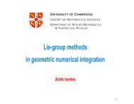
Left: three orbits <strong>of</strong> Kahan’s <strong>discretization</strong> with ɛ = 0.1,<br />
right: one orbit <strong>of</strong> the explicit Euler with ɛ = 0.01.<br />
◮ J.M. Sanz-Serna. An unconventional symplectic integrator<br />
<strong>of</strong> W.Kahan. Applied Numer. Math. 16 (1994) 245–250.<br />
A sort <strong>of</strong> an explanation <strong>of</strong> a non-spiralling behavior: Kahan’s<br />
integrator for the Lotka-Volterra system is symplectic (Poisson).<br />
Yuri B. Suris Kahan-Hirota-Kimura Discretizations
The problem <strong>of</strong> integrable <strong>discretization</strong>. Hamiltonian<br />
approach (Birkhäuser, 2003)<br />
Consider a completely integrable flow<br />
˙x = f (x) = {H, x} (1)<br />
with a Hamilton function H on a Poisson manifold P with a<br />
Poisson bracket {·, ·}. Thus, the flow (1) possesses many<br />
functionally independent integrals Ik(x) in involution.<br />
The problem <strong>of</strong> integrable <strong>discretization</strong>: find a family <strong>of</strong><br />
diffeomorphisms P → P,<br />
x = Φ(x; ɛ), (2)<br />
depending smoothly on a small parameter ɛ > 0, with the<br />
following properties:<br />
Yuri B. Suris Kahan-Hirota-Kimura Discretizations
1. The maps (2) approximate the flow (1):<br />
Φ(x; ɛ) = x + ɛf (x) + O(ɛ 2 ).<br />
2. The maps (2) are Poisson w. r. t. the bracket {·, ·} or some<br />
its deformation {·, ·}ɛ = {·, ·} + O(ɛ).<br />
3. The maps (2) are integrable, i.e. possess the necessary<br />
number <strong>of</strong> independent integrals in involution,<br />
Ik(x; ɛ) = Ik(x) + O(ɛ).<br />
While integrable lattice systems (like Toda or Volterra lattices)<br />
can be discretized in a systematic way (based, e.g., on the<br />
r-matrix structure), there is no systematic way to obtain decent<br />
integrable <strong>discretization</strong>s for integrable systems <strong>of</strong> classical<br />
mechanics.<br />
Yuri B. Suris Kahan-Hirota-Kimura Discretizations
Missing in the book: Hirota-Kimura <strong>discretization</strong>s<br />
◮ R.Hirota, K.Kimura. Discretization <strong>of</strong> the Euler top. J. Phys.<br />
Soc. Japan 69 (2000) 627–630,<br />
◮ K.Kimura, R.Hirota. Discretization <strong>of</strong> the Lagrange top. J.<br />
Phys. Soc. Japan 69 (2000) 3193–3199.<br />
Reasons for this omission: <strong>discretization</strong> <strong>of</strong> the Euler top<br />
seemed to be an isolated curiosity; <strong>discretization</strong> <strong>of</strong> the<br />
Lagrange top seemed to be completely incomprehensible, if not<br />
even wrong.<br />
Renewed interest stimulated by a talk by T. Ratiu at the<br />
Oberwolfach Workshop “Geometric Integration”, March 2006,<br />
who claimed that HK-type <strong>discretization</strong>s for the Clebsch<br />
system and for the Kovalevsky top are also integrable.<br />
Yuri B. Suris Kahan-Hirota-Kimura Discretizations
Hirota-Kimura’s discrete time Euler top<br />
⎧<br />
⎪⎨<br />
⎪⎩<br />
Features:<br />
˙x1 = α1x2x3,<br />
˙x2 = α2x3x1,<br />
˙x3 = α3x1x2,<br />
<br />
⎧<br />
⎪⎨<br />
⎪⎩<br />
x1 − x1 = ɛα1(x2x3 + x2 x3),<br />
x2 − x2 = ɛα2(x3x1 + x3 x1),<br />
x3 − x3 = ɛα3(x1x2 + x1 x2).<br />
◮ Equations are linear w.r.t. x = (x1, x2, x3) T :<br />
A(x, ɛ)x = x,<br />
⎛<br />
1<br />
A(x, ɛ) = ⎝−ɛα2x3<br />
−ɛα1x3<br />
1<br />
⎞<br />
−ɛα1x2<br />
−ɛα2x1⎠<br />
,<br />
−ɛα3x2 −ɛα3x1 1<br />
result in an explicit (rational) map, which is reversible<br />
(therefore birational):<br />
x = f (x, ɛ) = A −1 (x, ɛ)x, f −1 (x, ɛ) = f (x, −ɛ).<br />
Yuri B. Suris Kahan-Hirota-Kimura Discretizations
◮ Explicit formulas rather messy:<br />
⎧<br />
⎪⎨<br />
⎪⎩<br />
x1 = x1 + 2ɛα1x2x3 + ɛ2x1(−α2α3x 2 1 + α3α1x 2 2 + α1α2x 2 3 )<br />
∆(x, ɛ)<br />
x2 = x2 + 2ɛα2x3x1 + ɛ2x2(α2α3x 2 1 − α3α1x 2 2 + α1α2x 2 3 )<br />
,<br />
∆(x, ɛ)<br />
x3 = x3 + 2ɛα3x1x2 + ɛ2x3(α2α3x 2 1 + α3α1x 2 2 − α1α2x 2 3 )<br />
,<br />
∆(x, ɛ)<br />
where ∆(x, ɛ) = det A(x, ɛ)<br />
= 1 − ɛ 2 (α2α3x 2 1 + α3α1x 2 2 + α1α2x 2 3 ) − 2ɛ3 α1α2α3x1x2x3.<br />
(Try to see reversibility directly from these formulas!)<br />
Yuri B. Suris Kahan-Hirota-Kimura Discretizations<br />
,
◮ Two independent integrals:<br />
I1(x, ɛ) = 1 − ɛ2α2α3x 2 1<br />
1 − ɛ2α3α1x 2 , I2(x, ɛ) =<br />
2<br />
1 − ɛ2α3α1x 2 2<br />
1 − ɛ2α1α2x 2 .<br />
3<br />
◮ Invariant volume form:<br />
ω = dx1 ∧ dx2 ∧ dx3<br />
, φ(x) = 1 − ɛ<br />
φ(x)<br />
2 αiαjx 2 k<br />
and bi-Hamiltonian structure found in:<br />
M. Petrera, Yu. Suris. On the Hamiltonian structure <strong>of</strong> the<br />
Hirota-Kimura <strong>discretization</strong> <strong>of</strong> the Euler top. Math. Nachr.,<br />
2010, 283, 1654–1663, arXiv:0707.4382 [math-ph].<br />
Yuri B. Suris Kahan-Hirota-Kimura Discretizations
Hirota-Kimura’s discrete time Lagrange top<br />
Equations <strong>of</strong> motion <strong>of</strong> the Lagrange top:<br />
˙m1 = (α − 1)m2m3 + γp2,<br />
˙m2 = (1 − α)m1m3 − γp1,<br />
˙m3 = 0,<br />
˙p1 = αp2m3 − p3m2,<br />
˙p2 = p3m1 − αp1m3,<br />
˙p3 = p1m2 − p2m1.<br />
It is Hamiltonian w.r.t. Lie-Poisson bracket <strong>of</strong> e(3), has four<br />
functionally independent integrals in involution: two Casimir<br />
functions,<br />
C1 = p 2 1 + p2 2 + p2 3 , C2 = m1p1 + m2p2 + m3p3,<br />
the Hamilton function, and the (trivial) “fourth integral”,<br />
H1 = 1<br />
2 (m2 1 + m2 2 + αm2 3 ) + γp3, H2 = m3.<br />
Yuri B. Suris Kahan-Hirota-Kimura Discretizations
Discretization:<br />
m1 − m1 = ɛ(α − 1)( m2m3 + m2 m3) + ɛγ(p2 + p2),<br />
m2 − m2 = ɛ(1 − α)( m1m3 + m1 m3) − ɛγ(p1 + p1),<br />
m3 − m3 = 0,<br />
p1 − p1 = ɛα(p2 m3 + p2m3) − ɛ(p3 m2 + p3m2),<br />
p2 − p2 = ɛ(p3 m1 + p3m1) − ɛα(p1 m3 + p1m3),<br />
p3 − p3 = ɛ(p1 m2 + p1m2 − p2 m1 − p2m1).<br />
As usual, this gives an explicit birational map ( m, p) = f (m, p, ɛ).<br />
The trivial conserved quantity m3 = const. Quite nontrivial to<br />
find any further conserved quantity!<br />
Yuri B. Suris Kahan-Hirota-Kimura Discretizations
Hirota-Kimura’s “method” for finding integrals<br />
Consider the expression A = m2 1 + m2 2 − Bp3 − Cp2 3 , and<br />
determine A, B, C by requiring that they are conserved<br />
quantities. For this aim, solve the system <strong>of</strong> three equations for<br />
these three unknowns:<br />
⎧<br />
⎪⎨ A + Bp3 + Cp<br />
⎪⎩<br />
2 3 = m 2 1 + m 2 2 ,<br />
A + Bp3 + Cp2 3 = m2 1 + m2 2 ,<br />
A + B p<br />
3 + C p2<br />
3<br />
<br />
= m2 1<br />
<br />
+ m2 2<br />
<br />
with ( m, p) = f (m, p, ɛ) and ( m, p)<br />
= f<br />
<br />
−1 (m, p, ɛ). Then check<br />
that A, B, C = A, B, C(m, p, ɛ) are conserved quantities, indeed.<br />
Proceed similarly to determine the conserved quantities<br />
D, . . . , M from<br />
D = m1p1 + m2p2 − Ep3 − Fp 2 3 , K = p2 1 + p2 2 − Lp3 − Mp 2 3 .<br />
Does this make any sense for you???<br />
Yuri B. Suris Kahan-Hirota-Kimura Discretizations
Nevertheless, Hirota-Kimura’s “method” turns out to be valid in<br />
this case and also for remarkably many other Hirota-Kimura<br />
type <strong>discretization</strong>s.<br />
How should it be interpreted? Solve (symbolically) the system<br />
(A + Bp3 + Cp 2 3 ) ◦ f i (m, p, ɛ) = (m 2 1 + m2 2 ) ◦ f i (m, p, ɛ)<br />
with i = −1, 0, 1. Verify that A = A ◦ f , B = B ◦ f , C = C ◦ f .<br />
Alternatively, solve another copy <strong>of</strong> the above system with<br />
i = 0, 1, 2, and check that the solutions coincide. But then this<br />
system should be satisfied for all i ∈ Z. In other words, for any<br />
(m, p) ∈ R 6 , certain linear combination<br />
A + Bp3 + Cp 2 3 − (m2 1 + m2 2 )<br />
vanishes along the orbit <strong>of</strong> (m, p) under the map f .<br />
This is a very special feature <strong>of</strong> both the map f and the set <strong>of</strong><br />
functions (1, p3, p2 3 , m2 1 + m2 2 ). Also the sets <strong>of</strong> functions<br />
(1, p3, p 2 3 , m1p1 + m2p2), (1, p3, p 2 3 , p2 1 + p2 2 )<br />
have this property. It is formalized in the following definition.<br />
Yuri B. Suris Kahan-Hirota-Kimura Discretizations
Hirota-Kimura bases<br />
Definition. For a given birational map f : R n → R n , a set <strong>of</strong><br />
functions Φ = (ϕ1, . . . , ϕl), linearly independent over R, is<br />
called a HK-basis, if for every x0 ∈ R n there exists a <strong>vector</strong><br />
c = (c1, . . . , cl) = 0 such that<br />
c1ϕ1(f i (x0)) + . . . + clϕl(f i (x0)) = 0 ∀i ∈ Z.<br />
For a given x0 ∈ R n , the set <strong>of</strong> all <strong>vector</strong>s c ∈ R l with this<br />
property will be denoted by KΦ(x0) and called the null-space <strong>of</strong><br />
the basis Φ (at the point x0). This set clearly is a <strong>vector</strong> space.<br />
Note: we cannot claim that h = c1ϕ1 + ... + clϕl is an integral <strong>of</strong><br />
motion, since <strong>vector</strong>s c ∈ KΦ(x0) vary from one initial point x0 to<br />
another.<br />
However: existence <strong>of</strong> a HK-basis Φ with dim KΦ(x0) = d<br />
confines the orbits <strong>of</strong> f to (n − d)-dimensional invariant sets.<br />
Yuri B. Suris Kahan-Hirota-Kimura Discretizations
From HK-bases to integrals<br />
Proposition. If Φ is a HK-basis for a map f , then<br />
KΦ(f (x0)) = KΦ(x0).<br />
Thus, the d-dimensional null-space KΦ(x0) is a Gr(d, l)-valued<br />
integral. Its Plücker coordinates are scalar integrals.<br />
Especially simple is the situation when the null-space <strong>of</strong> a<br />
HK-basis has dimension d = 1.<br />
Corollary. Let Φ be a HK-basis for f with dim KΦ(x0) = 1 for all<br />
x0 ∈ R n . Let KΦ(x0) = [c1(x0) : . . . : cl(x0)] ∈ RP l−1 . Then the<br />
functions cj/ck are integrals <strong>of</strong> motion for f .<br />
In other words, normalizing cl(x0) = 1 (say), we find that all<br />
other cj (j = 1, . . . , l − 1) are integrals <strong>of</strong> motion. It is not clear<br />
whether one can say something general about the number <strong>of</strong><br />
functionally independent integrals among them. It varies in<br />
examples (sometimes just = 1 and sometimes > 1).<br />
Yuri B. Suris Kahan-Hirota-Kimura Discretizations
Hirota-Kimura bases for the discrete Lagrange top<br />
Thus, results by Hirota and Kimura in the Lagrange top case<br />
can be put as follows:<br />
Theorem. The three sets <strong>of</strong> functions,<br />
Φ1 = (m 2 1 + m2 2 , p2 3 , p3, 1),<br />
Φ2 = (m1p1 + m2p2, p 2 3 , p3, 1),<br />
Φ3 = (p 2 1 + p2 2 , p2 3 , p3, 1),<br />
are HK-bases for the discrete time Lagrange top with<br />
one-dimensional null-spaces.<br />
It follows that any orbit lies on a two-dimensional surface in R 6<br />
which is intersection <strong>of</strong> three quadrics and a hyperplane<br />
m3 = const .<br />
Yuri B. Suris Kahan-Hirota-Kimura Discretizations
An impression about the complexity <strong>of</strong> the integrals thus found<br />
can be given by this: KΦ 1 (x) = [c0 : c1 : c2 : −1], with<br />
c0 = m2 1 + m2 2 + 2γp3 + ɛ2c (4)<br />
0 + ɛ4c (6)<br />
0 + ɛ6c (8)<br />
0 + ɛ8c (10)<br />
0<br />
∆1∆2<br />
(and similar expressions for c1, c2), where<br />
coefficients ∆ (q) and c (q)<br />
k<br />
phase variables.<br />
∆1 = 1 + ɛ 2 α(1 − α)m 2 3 − ɛ2 γp3,<br />
∆2 = 1 + ɛ 2 ∆ (2)<br />
2 + ɛ4 ∆ (4)<br />
2 + ɛ6 ∆ (6)<br />
2 ;<br />
are polynomials <strong>of</strong> degree q in the<br />
Yuri B. Suris Kahan-Hirota-Kimura Discretizations<br />
,
A simple integral (unnoticed by Hirota and Kimura) is given by:<br />
Theorem. The set<br />
Γ = ( m1p1 − m1 p1, m2p2 − m2 p2, m3p3 − m3 p3)<br />
is a HK-basis for the discrete time Lagrange top with<br />
one-dimensional null-space KΓ(x) = [1 : 1 : I ],<br />
I = (2α − 1) + ɛ2 (α − 1)(m2 1 + m2 2 ) + ɛ2γ(m1p1 + m2p2)/m3<br />
1 + ɛ2α(1 − α)m2 3 − ɛ2 .<br />
γp3<br />
Another result which was unknown to Hirota and Kimura reads:<br />
Theorem. The discrete time Lagrange top possesses an<br />
invariant volume form:<br />
f ∗ ω = ω, ω = dm1 ∧ dm2 ∧ dm3 ∧ dp1 ∧ dp2 ∧ dp3<br />
.<br />
∆2(m, p)<br />
Yuri B. Suris Kahan-Hirota-Kimura Discretizations
Further examples <strong>of</strong> integrable HK-<strong>discretization</strong>s<br />
Work in progress with A. Pfadler, M. Petrera. An overview given<br />
in arXiv:1008.1040 [nlin.SI] (to appear in Regular and<br />
Chaotic Dyn.). An (incomplete) list <strong>of</strong> examples:<br />
◮ Three-wave interaction system.<br />
◮ Periodic Volterra chain <strong>of</strong> period N = 3, 4:<br />
◮ Dressing chain with N = 3:<br />
˙xk = xk(xk+1 − xk−1), k ∈ Z/NZ<br />
˙xk + ˙xk+1 = x 2 k+1 − x 2 k + αk+1 − αk, k ∈ Z/NZ, N odd.<br />
◮ System <strong>of</strong> two interacting Euler tops.<br />
◮ Kirchh<strong>of</strong> and Clebsch cases <strong>of</strong> the rigid body motion in an<br />
ideal fluid.<br />
Yuri B. Suris Kahan-Hirota-Kimura Discretizations
Clebsch case<br />
Clebsch case <strong>of</strong> the motion <strong>of</strong> a rigid body in an ideal fluid:<br />
˙m1 = (ω3 − ω2)p2p3,<br />
˙m2 = (ω1 − ω3)p3p1,<br />
˙m3 = (ω2 − ω1)p1p2,<br />
˙p1 = m3p2 − m2p3,<br />
˙p2 = m1p3 − m3p1,<br />
˙p3 = m2p1 − m1p2.<br />
It is Hamiltonian w.r.t. Lie-Poisson bracket <strong>of</strong> e(3), has four<br />
functionally independent integrals in involution:<br />
Ii = p 2 i + m2 j<br />
ωk − ωi<br />
and H4 = m1p1 + m2p2 + m3p3.<br />
+ m2 k , (i, j, k) = c.p.(1, 2, 3),<br />
ωj − ωi<br />
Yuri B. Suris Kahan-Hirota-Kimura Discretizations
Hirota-Kimura <strong>discretization</strong> <strong>of</strong> the Clebsch system<br />
Hirota-Kimura-type <strong>discretization</strong> (proposed by T. Ratiu on<br />
Oberwolfach Meeting “Geometric Integration”, March 2006):<br />
m1 − m1 = ɛ(ω3 − ω2)(p2p3 + p2 p3),<br />
m2 − m2 = ɛ(ω1 − ω3)(p3p1 + p3 p1),<br />
m3 − m3 = ɛ(ω2 − ω1)(p1p2 + p1 p2),<br />
p1 − p1 = ɛ( m3p2 + m3 p2) − ɛ( m2p3 + m2 p3),<br />
p2 − p2 = ɛ( m1p3 + m1 p3) − ɛ( m3p1 + m3 p1),<br />
p3 − p3 = ɛ( m2p1 + m2 p1) − ɛ( m1p2 + m1 p2).<br />
What follows is based on: M. Petrera, A. Pfadler, Yu. Suris. On<br />
integrability <strong>of</strong> Hirota-Kimura type <strong>discretization</strong>s. Experimental<br />
study <strong>of</strong> the discrete Clebsch system. Experimental Math.,<br />
2009, 18, 223–247, arXiv:0808.3345 [nlin.SI]<br />
Yuri B. Suris Kahan-Hirota-Kimura Discretizations
A birational map<br />
<br />
m<br />
= f (m, p, ɛ) = M<br />
p<br />
−1 <br />
m<br />
(m, p, ɛ) ,<br />
p<br />
⎛<br />
1 0 0 0 ɛω23p3 ɛω23p2<br />
0 1 0 ɛω31p3 0 ɛω31p1<br />
⎜<br />
M(m, p, ɛ) = ⎜ 0<br />
⎜ 0<br />
⎝−ɛp3<br />
0<br />
ɛp3<br />
0<br />
1<br />
−ɛp2<br />
ɛp1<br />
ɛω12p2<br />
1<br />
ɛm3<br />
ɛω12p1<br />
−ɛm3<br />
1<br />
0<br />
ɛm2<br />
−ɛm1<br />
ɛp2 −ɛp1 0 −ɛm2 ɛm1 1<br />
with ωij = ωi − ωj. The usual reversibility:<br />
f −1 (m, p, ɛ) = f (m, p, −ɛ).<br />
Numerators and denominators <strong>of</strong> components <strong>of</strong> m, p are<br />
polynomials <strong>of</strong> degree 6, the numerators <strong>of</strong> pi consist <strong>of</strong> 31<br />
monomials, the numerators <strong>of</strong> mi consist <strong>of</strong> 41 monomials, the<br />
common denominator consists <strong>of</strong> 28 monomials.<br />
Yuri B. Suris Kahan-Hirota-Kimura Discretizations<br />
⎞<br />
⎟ ,<br />
⎟<br />
⎠
Phase portraits<br />
1<br />
0.5<br />
0<br />
−0.5<br />
−1<br />
1<br />
0.5<br />
0<br />
−0.5<br />
−1<br />
1<br />
0.95<br />
0.9<br />
0.85<br />
0.8<br />
0.75<br />
0.7<br />
0.65<br />
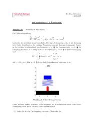
An orbit <strong>of</strong> the discrete Clebsch system with ω1 = 0.1, ω2 = 0.2,<br />
ω3 = 0.3 and ɛ = 1; projections to (m1, m2, m3) and to<br />
(p1, p2, p3); initial point (m0, p0) = (1, 1, 1, 1, 1, 1).<br />
0.5<br />
0.4<br />
0.3<br />
0.2<br />
0.1<br />
0<br />
−0.1<br />
−0.2<br />
−0.3<br />
−0.4<br />
−0.5<br />
0.8<br />
Yuri B. Suris Kahan-Hirota-Kimura Discretizations<br />
0.6<br />
0.4<br />
0.2<br />
0<br />
−0.2<br />
−0.4<br />
−0.6<br />
−0.8<br />
0.5<br />
1<br />
1.5
−10 −8 −6 −4 −2 0 2 4 6 8<br />
0<br />
10<br />
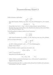
An orbit <strong>of</strong> the discrete Clebsch system with ω1 = 1, ω2 = 0.2,<br />
ω3 = 30 and ɛ = 1; projections to (m1, m2, m3) and to<br />
(p1, p2, p3); initial point (m0, p0) = (1, 1, 1, 1, 1, 1).<br />
−1.5<br />
−1<br />
−0.5<br />
0<br />
0.5<br />
1<br />
1.5<br />
1.5<br />
1<br />
0.5<br />
0<br />
−0.5<br />
−1<br />
−1.5<br />
2.5<br />
Yuri B. Suris Kahan-Hirota-Kimura Discretizations<br />
2<br />
1.5<br />
1<br />
0.5<br />
0<br />
−0.5<br />
−3<br />
−2<br />
−1<br />
0<br />
1<br />
2<br />
3
Results for the discrete Clebsch system<br />
Theorem. a) The set <strong>of</strong> functions<br />
Φ = (p 2 1 , p2 2 , p2 3 , m2 1 , m2 2 , m2 3 , m1p1, m2p2, m3p3, 1)<br />
is a HK-basis for f , with dim KΦ(m, p) = 4. Thus, any orbit <strong>of</strong> f<br />
lies on an intersection <strong>of</strong> four quadrics in R 6 .<br />
b) The following four sets <strong>of</strong> functions are HK-bases for f with<br />
one-dimensional null-spaces:<br />
Φ0 = (p 2 1 , p2 2 , p2 3 , 1),<br />
Φ1 = (p 2 1 , p2 2 , p2 3 , m2 1 , m2 2 , m2 3 , m1p1),<br />
Φ2 = (p 2 1 , p2 2 , p2 3 , m2 1 , m2 2 , m2 3 , m2p2),<br />
Φ3 = (p 2 1 , p2 2 , p2 3 , m2 1 , m2 2 , m2 3 , m3p3).<br />
There holds: KΦ = KΦ 0 ⊕ KΦ 1 ⊕ KΦ 2 ⊕ KΦ 3 .<br />
Yuri B. Suris Kahan-Hirota-Kimura Discretizations
HK-basis Φ0<br />
Theorem. At each point (m, p) ∈ R6 there holds:<br />
<br />
1<br />
KΦ (m, p) =<br />
0 + ɛ 2 ω1 : 1<br />
+ ɛ 2 ω2 : 1<br />
where<br />
J0<br />
J0<br />
+ ɛ<br />
J0<br />
2 ω3 : −1<br />
p<br />
J0(m, p, ɛ) =<br />
2 1 + p2 2 + p2 3<br />
1 − ɛ2 (ω1p2 1 + ω2p2 2 + ω3p2 .<br />
3 )<br />
This function is an integral <strong>of</strong> motion <strong>of</strong> the map f .<br />
This is the only “simple” integral <strong>of</strong> f !<br />
Yuri B. Suris Kahan-Hirota-Kimura Discretizations<br />
<br />
,
HK-bases Φ1, Φ2, Φ3<br />
Theorem. At each point (m, p) ∈ R 6 there holds:<br />
KΦ 1 (m, p) = [α1 : α2 : α3 : α4 : α5 : α6 : −1],<br />
KΦ 2 (m, p) = [β1 : β2 : β3 : β4 : β5 : β6 : −1],<br />
KΦ 3 (m, p) = [γ1 : γ2 : γ3 : γ4 : γ5 : γ6 : −1],<br />
where αj,βj, and γj are rational functions <strong>of</strong> (m, p), even with<br />
respect to ɛ. They are integrals <strong>of</strong> motion <strong>of</strong> the map f . For<br />
j = 1, 2, 3 they are <strong>of</strong> the form<br />
h = h(2) + ɛ 2 h (4) + ɛ 4 h (6) + ɛ 6 h (8) + ɛ 8 h (10) + ɛ 10 h (12)<br />
2ɛ 2 (p 2 1 + p2 2 + p2 3 )∆<br />
∆ = m1p1 + m2p2 + m3p3 + ɛ 2 ∆ (4) + ɛ 4 ∆ (6) + ɛ 6 ∆ (8) ,<br />
where h stands for any <strong>of</strong> the functions αj, βj, γj, j = 1, 2, 3, and<br />
the corresponding h (2q) and ∆ (2q) are homogeneous<br />
polynomials in phase variables <strong>of</strong> degree 2q. For instance,<br />
Yuri B. Suris Kahan-Hirota-Kimura Discretizations<br />
,
HK-bases Φ1, Φ2, Φ3 (continued)<br />
α (2)<br />
1 = H3 − I1, α (2)<br />
2 = −I1, α (2)<br />
3 = −I1,<br />
β (2)<br />
1 = −I2, β (2)<br />
2 = H3 − I2, β (2)<br />
3<br />
= −I2,<br />
γ (2)<br />
1 = −I3, γ (2)<br />
2 = −I3, γ (2)<br />
3 = H3 − I3,<br />
where H3 = p 2 1 + p2 2 + p2 3 . The four integrals J0, α1, β1 and γ1<br />
are functionally independent.<br />
Yuri B. Suris Kahan-Hirota-Kimura Discretizations
Complexity issues<br />
The claims <strong>of</strong> the last two theorems refer to the solutions <strong>of</strong> the<br />
following systems:<br />
(c1p 2 1 + c2p 2 2 + c3p 2 3 ) ◦ f i = 1,<br />
(α1p 2 1 + α2p 2 2 + α3p 2 3 + α4m 2 1 + α5m 2 2 + α6m 2 3 ) ◦ f i = m1p1 ◦ f i ,<br />
(β1p 2 1 + β2p 2 2 + β3p 2 3 + β4m 2 1 + β5m 2 2 + β6m 2 3 ) ◦ f i = m2p2 ◦ f i ,<br />
(γ1p 2 1 + γ2p 2 2 + γ3p 2 3 + γ4m 2 1 + γ5m 2 2 + γ6m 2 3 ) ◦ f i = m3p3 ◦ f i .<br />
The first one has to be solved for one non-symmetric range <strong>of</strong><br />
l − 1 = 3 values <strong>of</strong> i, or for two different such ranges. The last<br />
three systems have to be solved for a non-symmetric range <strong>of</strong><br />
l − 1 = 6 values <strong>of</strong> i. This can be done numerically (in rational<br />
arithmetic) without any difficulties, but becomes (nearly)<br />
impossible for a symbolic computation, due to complexity <strong>of</strong> f 2 .<br />
Yuri B. Suris Kahan-Hirota-Kimura Discretizations
Complexity <strong>of</strong> f 2<br />
Degrees <strong>of</strong> numerators and denominators <strong>of</strong> f 2 :<br />
Denom. <strong>of</strong> f 2<br />
Num. <strong>of</strong> p1 ◦ f 2<br />
Num. <strong>of</strong> p2 ◦ f 2<br />
Num. <strong>of</strong> p3 ◦ f 2<br />
Num. <strong>of</strong> m1 ◦ f 2<br />
Num. <strong>of</strong> m2 ◦ f 2<br />
Num. <strong>of</strong> m3 ◦ f 2<br />
deg<br />
27<br />
degp1 24<br />
degp2 24<br />
degp3 24<br />
degm1 12<br />
degm2 12<br />
degm3 12<br />
27 25 24 24 12 12 12<br />
27 24 25 24 12 12 12<br />
27 24 24 25 12 12 12<br />
33 28 28 28 15 14 14<br />
33 28 28 28 14 15 14<br />
33 28 28 28 14 14 15<br />
The numerator <strong>of</strong> the p1-component <strong>of</strong> f 2 (m, p), as a<br />
polynomial <strong>of</strong> mk, pk, contains 64 056 monomials; as a<br />
polynomial <strong>of</strong> mk, pk, and ωk, it contains 1 647 595 terms.<br />
Need new ideas! The main one: find (observe numerically)<br />
linear relations between the components <strong>of</strong> KΦ(x0), and then<br />
use them to replace the dynamical relations.<br />
Yuri B. Suris Kahan-Hirota-Kimura Discretizations
Example<br />
Plotting solutions (c1, c2, c3) <strong>of</strong> the system<br />
(c1p 2 1 + c2p 2 2 + c3p 2 3 ) ◦ f i = 1, i = 0, 1, 2<br />
with varying initial data, we get:<br />
0<br />
−5<br />
−10<br />
−15<br />
0<br />
−2<br />
−4<br />
−6<br />
−8<br />
Komp. 1,2,3<br />
Straight line two linear relations between (c1, c2, c3)!<br />
−10<br />
−12<br />
−14<br />
−15<br />
Yuri B. Suris Kahan-Hirota-Kimura Discretizations<br />
−10<br />
−5<br />
0
Summary for the Clebsch system<br />
We established the integrability <strong>of</strong> the Hirota-Kimura<br />
<strong>discretization</strong> <strong>of</strong> the Clebsch system, in the sense <strong>of</strong><br />
◮ existence, for every initial point (m, p) ∈ R 6 , <strong>of</strong> a<br />
four-dimensional pencil <strong>of</strong> quadrics containing the orbit <strong>of</strong><br />
this point;<br />
◮ existence <strong>of</strong> four functionally independent integrals <strong>of</strong><br />
motion (conserved quantities).<br />
This remains true also for an arbitrary flow <strong>of</strong> the Clebsch<br />
system (with one “simple” and three very big integrals).<br />
Our pro<strong>of</strong>s are computer assisted. We did not find a general<br />
structure, which would provide us with less computational<br />
pro<strong>of</strong>s and with more insight. In particular, nothing like a Lax<br />
representation has been found. Nothing is known about the<br />
existence <strong>of</strong> an invariant Poisson structure for these maps.<br />
Yuri B. Suris Kahan-Hirota-Kimura Discretizations
Conjecture<br />
The previous discussion seems to support the following<br />
Conjecture. For any algebraically completely integrable system<br />
with a <strong>quadratic</strong> <strong>vector</strong> field, its Hirota-Kimura <strong>discretization</strong><br />
remains algebraically completely integrable<br />
pushed forward in our paper in “Exp. Math.”. However, at<br />
present we have a number <strong>of</strong> apparent counterexamples (it is<br />
extremely difficult to prove non-integrability), including the so<br />
called Zhukovsky-Volterra gyrostat. However, the HK<br />
<strong>discretization</strong> maintains integrability much more <strong>of</strong>ten than a<br />
mere coincidence would allow.<br />
The full story still has to be clarified.<br />
Yuri B. Suris Kahan-Hirota-Kimura Discretizations