Water Management Scenarios and Clams - Jan Thompson, U.S.G.S.

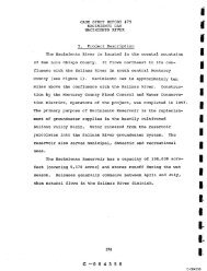
Chlorophyll a (μg/L)
60
50
40
30
20
10
0
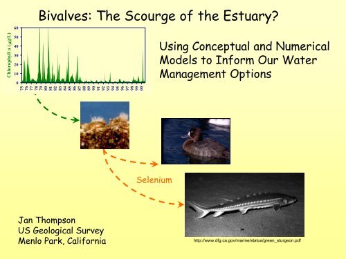
Bivalves: The Scourge of the Estuary?
75
76
77
78
79
80
81
82
83
84
85
86
87
88
89
90
91
92
93
94
95
96
97
98
99
00
Jan Thompson
US Geological Survey
Menlo Park, California
Selenium
Using Conceptual and Numerical
Models to Inform Our Water
Management Options
http://www.dfg.ca.gov/marine/status/green_sturgeon.pdf

My charge
Any good models on the shelf? No
How can we use conceptual models like those
developed in DRERIP? Strengths? Weaknesses?
How do conceptual models differ from numerical
models being developed in CASCADE? Strengths?
Weaknesses?
What’s the future for bivalve models?
Status:
Invaded 1986 and limited laboratory studies
DRERIP conceptual model
STELLA population model – not dynamically linked
Invaded 1940 and more laboratory studies
DRERIP conceptual model
STELLA population model – not dynamically linked

Bivalve models are connected to many submodels
but must be connected to hydrodynamic models
at a minimum to
Distribute gametes and young
Maintain/change water quality
Deliver food to the sedentary animals

Conceptual models such as DRERIP
models are critical for:
Designing numerical models – particularly
valuable in making connections between bivalves
and other factors (physical transport & mixing,
phytoplankton etc)
Highlighting data needs and prioritizing
research needs and dollars
Examining processes which may not be modeled
in the near term

DRERIP: We have developed Corbul and Corbicula Life
Cycle Models, the first step in building conceptual models
Reproductive
Adult
(5mm long)
Recruit
(135 µm long)
17-19 days
Corbula
Pelagic
Veliger
Larvae*
Spawning &
Fertilization
Pelagic
Trochophore
Larvae*
*From Nicolini, MH and DL Penry. 2000. Spawning, fertilization, and larval development of Potamocorbula amurensis (Mollusca: Bivalvia) from San Francisco Bay, California. Pacific Science:
54(4):377-388 NO PERMISSION FOR PUB.
24 hours
Gametogenesis
24 hours

DRERIP sub-models have been connected to each Life
Cycle Model and coded for habitat and critical processes
physical processes dominate
Adult
Transport
Model
Mortality
Model
Reproductive
Adult
(5mm long)
Growth
Model
Recruit
(135 µm long)
Larval
Recruit
Model
benthic habitat
17-19 days
pelagic habitat
Pelagic
Veliger
Larvae*
Mortality
Model
Gametogenesis
physical processes critical
Spawning &
Fertilization
Pelagic
Trochophore
Larvae*
Larval
Transport
Model
Reproduction
Model
*From Nicolini, MH and DL Penry. 2000. Spawning, fertilization, and larval development of Potamocorbula amurensis (Mollusca: Bivalvia) from San Francisco Bay, California. Pacific Science:
54(4):377-388 NO PERMISSION FOR PUB.
24 hours
24 hours

Each DRERIP sub-model includes triggers or forcing
factors and stressors
Food Quantity
Food Quality
Water Quality
Toxics
Adult Health
Water Quality
Adult Health
Water Quality
Gametogenesis
Internal
Fertilization
Release Brood
el.erdc.usace.army
Gametogenesis
Broadcast
Spawning
External
Fertilization
Pelagic
Trochophore
Larvae
Food Quantity
Food Quality
Water Quality
Toxics
Adult Health
Stress/ no food
Water Quality
Water Quality
Transport

DRERIP models help us build numerical models AND tell
us what we know, how well we know it, and what critical
data are lacking
Importance
High
Medium
Low
Understanding
High
Medium
Low
Predictability
High
Medium
Low
Food Quantity
Food Quality
Water Quality
Toxics
Adult Health
Water Quality
Adult Health
Water Quality
Gametogenesis
Internal
Fertilization
Release Brood
el.erdc.usace.army

A similar exercise for Corbula shows different data gaps
and needs
Importance
High
Medium
Low
Understanding
High
Medium
Low
Predictability
High
Medium
Low
Gametogenesis
Broadcast
Spawning
External
Fertilization
Pelagic
Trochophore
Larvae
Food Quantity
Food Quality
Water Quality
Toxics
Adult Health
Stress/ no food
Water Quality
Water Quality
Transport

Salinity
Food
35
30
25
20
15
10
5
0
Year Class 1 Gametogenesis
understanding of controls on a species distribution
0
Spawn
Fertilization
Days
1 2 17-19 80+ Fall
Spring Extended Life Cycle Models further our
Pelagic Larva
Pelagic Swimming Larva
Settled Juvenile
Some times &
places >1/season
Pelagic Infaunal
Reproductively Mature Adult
Year Class 2 Gametogenesis

Temperature
Food
35
30
25
20
15
10
5
0
Year Class 1 Oogenesis
And allow us to contrast controls on different
species
Always
Spring
Spermatogenesis
0
Self -Fertilization
Pediveliger
Days
Fall
5 7 12 17 19
90+
Spermatogenesis
Self -Fertilization
Pediveliger
Spermatogenesis
Stop when ≈26°C
or insufficient food
Epibenthic/Pelagic Infaunal
Juveniles Reproductively Mature
Year Class 2 Oogenesis
Spermatogenesis

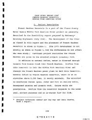
DRERIP can help us discover critical processes
before we are ready to model them. Eg. Eg.
Why do
the clams disappear in winter? Does it matter?
Net Outflow (m 3 /s)
600000
500000
400000
300000
200000
100000
0
Grizzly Bay Corbula
88 89 90 91 92 93 94 95 96 97 98 99 00 01 02 03 04 05 06
Samples courtesy of DWR (D7)
0.7
0.6
0.5
0.4
0.3
0.2
0.1
0.0
Corbula Biomass
(g AFDW/m 2 )

Migratory ducks heavily prey upon
shallow water Corbula Corbula and they are
bio-accumulating bio accumulating Se.
Mortality
Benthic Predation
Pelagic Larvae
Predation
Starvation
Burial
Water Quality Stress
Natural Death - Age
Fish
Resident Birds
Migratory Birds
Invertebrates
Corbula
Mortality
Model
White Sturgeon
Sacramento Splittail
Ducks
Opisthobranchs
Dungeness Crab
physical processes
dominate
physical processes
critical
biological variables

However DRERIP models can’t can t explain the inter-
annual variability in biomass (and thus grazing)
peaks
Net Outflow (m 3 /s)
600000
500000
400000
300000
200000
100000
0
Grizzly Bay Corbula
88 89 90 91 92 93 94 95 96 97 98 99 00 01 02 03 04 05 06
Samples courtesy of DWR (D7)
0.7
0.6
0.5
0.4
0.3
0.2
0.1
0.0
Corbula Biomass
(g AFDW/m 2 )

DRERIP models also can’t can t tell us why Corbicula Corbicula
juveniles occur throughout the Delta but only
grow-up grow up in the central Delta.

To do that we need to look at growth
models and it becomes obvious that we
need more than a conceptual model.
Tissue Growth
Energy for
Growth
Carbon Available
for Assimilation
Growth
(increase in
Carbon)
Shell Growth
Energy for
Reproduction
Energy for
Respiration
Energy for
Excretion
Consumption
Rate
Physiological
Stressors
Food Quality
Filtration Efficiency
Filtration Rate
Water Quality
Food Quantity
Suspended Sediment
Population Size of
Filter Feeders
Current Speed
Behavior
Pumping Rate
Zooplankton
Phytoplankton
Bacteria
DOM
Zooplankton
Phytoplankton
Bacteria
DOM
Corbula
Growth
Model
Water Quality
physical processes
dominate
physical processes
critical
biological variables
Species
Size
Species
Size
Attached/Free?
Size

In Summary, conceptual models such
as DRERIP models do not
Tell us the magnitude of the bivalves ecological
functions (eg. consuming phytoplankton)
Tell us the temporal and spatial variability of
those ecological functions, the causes of which
might be exploited by water management
Tell us if the model is wrong – surprises are when
we learn
Allow us to dynamically link and manipulate
variables

Numerical models within CASCADE
We are using STELLA models until we know
more – adapted to be spatially variable and
responsive to stressors
Will tell us about processes and limits on
populations – I will discuss some today
Allow us to dynamically link and manipulate some
variables
We expect and look forward to surprises

We are simplifying STELLA models to operate with
statistical relationships instead of using energetic
principles.
Standard Stella
Energetic Growth
Model
Statistical Stella
Growth Model
Adapted from Grant and Bacher 1998

Spatial resolution and physical variables known to
dynamically interact with clam functions will be run
sequentially to produce a “look up” table for other
models.
habitat
1
.
.
.
.
.
.
.
20
1 . . . . . 5
phytoplankton
biomass
1 . . . . . 4
temperature
Output: Temporally and spatially
varying growth rate, biomass,
grazing rate for phytoplankton and
contaminant models

Step 1: Initial Conditions: Where are the two species in
space? Corbula recruits settle downstream of X2
(Corbicula juveniles settle upstream of X2!)
X2 at 4.1 # Recruits/0.05m2
physical processes dominate
# Adults/0.05m 2
1000
900
800
700
600
500
400
300
200
100
0
200
180
160
140
120
100
80
60
40
20
0
station is at X2 of 72; as
long as X2 meets or exceeds
that level we get recruits
40 45 50 55 60 65 70 75 80 85 90 95 100
Older year class shows wider
spread which we expect
because they are tolerant of
lower salinities
40 45 50 55 60 65 70 75 80 85 90 95 100

In order to establish some statistical bounds to our
results, we will use an ensemble of salinity and
temperature distributions in time and space to establish
a range of distributions for each scenario
ΔWater Temp / ΔAir Temp
0.65
0.6
0.55
0.5
0.45
0.4
-122.3 -122.2 -122.1 -122 -121.9 -121.8
Longitude
-121.7 -121.6 -121.5 -121.4 -121.3
Grantline Tracy
SJ Antioch
Middle Tracy
SJ Prisoner
Wickland Pier
Sac Martinez
Stockton Burns
Old Tracy
SJ Navy Bridge
Sac Mallard
SJ Mossdale
Sac Rio Vista
Sac Hood
Preliminary data from Wayne Wagner & Mark Stacey

physical processes critical
biological variables
Initial Conditions: Number of recruits is
partially dependent on the biomass of adults
present; there is a physical and biological basis
for this relationship
# Recruits/0.05m 2
1400
1200
1000
800
600
400
200
0
0 0.2 0.4 0.6 0.8
Biomass Adults/0.05m 2

Net Outflow (m 3 /s)
600000
500000
400000
300000
200000
100000
We assign Corbula recruit abundance based on
biomass of adults and antecedent outflow
events – note the grouping of abundances
around 100, 200 and

# Recruits ( ≤2.5 mm/0.05m 2 )
# Recruits ( ≤2.5 mm/0.05m 2 )
80
70
60
50
40
30
20
10
0
350
300
250
200
150
100
50
0
Apr
Jan-98
May
Apr-98
We observe Corbicula recruit abundance at
≈20 recruits/0.05 m2 throughout the year at
monitoring stations
Franks Tract Near Old River
Jun
Jul-98
Jul
Oct-98
Aug
Jan-99
Sep
Apr-99
Oct
Jul-99
Nov
Oct-99
Dec
Jan-00
Jan
Sacramento River Near Rio Vista
No data
Apr-00
Feb
Jul-00
Mar
Oct-00
We are determining if transport
of larvae from non-local sites,
where temperature regimes may
be staggered, accounts for the
near continuous pattern of
recruitment observed in areas like
the central delta where many
sources of water are mixed.
If so changing temperatures
throughout the tributaries and
Delta could alter this population
distribution
physical processes critical

Corbicula’s present and potential biomass
distribution is likely based on food limitation so a
growth relationship is critical to our model
Feb-Dec 1981
Foe & Knight 1985
Corbicula growth is food limited at
20 mg/L chlorophyll a at 15°C and 47
mg/L at 20-24°C. Growth was limited
in the San Joaquin River except for two
months in 1981 so this relationship is
probably as good as is available for this
system
Chlorophyll a
(mg/L)
30
25
20
15
10
5
0
San Joaquin River at Antioch Ship Channel
Jan Feb Mar Apr Ma
y
Jun Jul Aug Sep Oct Nov Dec
physical processes critical

Shell Length
Growth Rate
(mm/d)
We believe that Corbula is also food limited in
this system but we do not have laboratory data
similar to that for Corbicula to verify our beliefs.
0.08
0.07
0.06
0.05
0.04
0.03
0.02
0.01
0
y = 0.0121e 0.6072x
R 2 = 0.9791
Recruits in Grizzly Bay
0 0.5 1 1.5 2 2.5 3
Average Chlorophyll a (mg/L)
Our preliminary analyses of field data confirm food
limitation in bivalves in the shallow water.

Summary
Our skill with both bivalve models is limited by
data
Data gaps and priorities are well summarized by
conceptual models (DRERIP)
Developing relationships for use in the numerical
models is ongoing and is helping us define important
processes and thresholds
Given the best data and models, ecologists are
still struggling with multi-generation, spatially
explicit population models of benthic animals. We
also expect to have problems so we are taking it
slow, linking sub-models one step at a time

Net Outflow (m 3 /s)
Net Outflow (m 3 /s)
600000
500000
400000
300000
200000
100000
0
600000
500000
400000
300000
200000
100000
0
800+
87 88 89 90 91 92 93 94 95 96 97 98 99 00 01 02 03 04 05 06
87 88 89 90 91 92 93 94 95 96 97 98 99 00 01 02 03 04 05 06
500
400
300
200
100
0
0.7
0.6
0.5
0.4
0.3
0.2
0.1
0.0
# Recruits (/0.05m 2 )
Adult Corbula Biomass
(g AFDW/m 2 )