135 - Combustion Institute British Section

Experiments with Progress Variable Approach in the Contest of
Large Eddy Simulation for Combustion
Rajani Kumar Akula*, Amsini Sadiki, Johannes Janicka
Chair of Energy and Powerplant Technology, TU-Darmstadt, Germany
Petersenstr. 30, Darmstadt, Germany-64287.
Tel.: +49 6151 165697, Fax: +49 6151 166555, Email: akula@ekt.tu-darmstadt.de
Abstract
The main aim of the present work is to investigate the influence of the different approaches
(based on the progress variable) on the behaviour of the premixed flame front prediction by using
Large Eddy Simulation. These approaches are thickened flame approach and explicit filter based
progress variable method. To this purpose a configuration providing the bluff body stabilized
flame has been used. As a first step velocity predictions are reported in this work.
Introduction
Large eddy simulations (LES) are now
viewed as a promising tool to address
combustion problems where classical
Reynolds-averaging numerical simulations
(RANS) approaches have proved to lack
precision or where the intrinsically unsteady
nature of the flow makes RANS clearly
inadequate. LES allows a better description
of the turbulence–combustion interactions
because, large structures are explicitly
computed and instantaneous fresh and burnt
gases zones, where turbulence characteristics
are quite different, are clearly identified [1].
But LES of premixed combustion is difficult
due to the thickness of the premixed flame
about 0.1–1 mm and generally smaller than
the LES mesh size. To overcome this
difficulty several approaches have been
developed, such as flame front tracking
techniques (e.g., the G equation [2–4]),
simulating filtered progress variables [5],
and the so called thickened flame approach
(TF-LES). In the later the diffusion and preexponential
factors in the Arrhenuis law
based reaction term are modified so as to
yield an artificially thickened flame [7–10].
However in all the techniques used, a model
is needed to account for the fact that the real
unresolved flame is wrinkled at scales below
the LES resolution, which typically provides
an increased surface area for the flame and
thus an increased reaction rate. This model is
introduced through the flame wrinkling
factor. To measure the influence of these
methods to capture the behaviour of the
premixed flame front, we consider the socalled
VOLVO test case referred as
Validation Rig 1 (VR 1), as detailed
experimental results are available. In this
paper we concentrate on the velocity
predictions for this case. For the simulations
we follow dynamic SGS model. Germano et
al. [11] developed a dynamic SGS model
(DSM) which overcomes some of the
aforementioned drawbacks of the
Smagorinsky model. This model has many
desirable features in that it requires only one
input parameter, i.e., ratio of test filter width
and grid filter. DSM has been successfully
applied to LES of transitional and turbulent
channel flows [11] and both incompressible
and compressible isotropic turbulence [12].
However, the dynamically computed model
coefficient was averaged either in the global
volume of the domain or in a homogeneous
plane. To overcome this problem Meneveau
et al. [12] has proposed a Lagrangian
dynamic model. In this work we have used
this Lagrangian dynamic model.
Numerical Procedure and Modelling
The governing equations are discretised on a
block structured boundary- fitted collocated
grid following the finite-volume approach.
Spatial discretisations are 2nd order with

flux blending technique for the convective
terms. The solution is updated in time using
2nd order accurate implicit Crank-Nicolson
scheme. A SIMPLE type pressure correction
is used for pressure-velocity coupling. The
resulting set of linear equations is solved
iteratively. Details of the method can be
found in the paper by Mengler et al. The
basic governing equations for LES of
premixed combustion are then the favre
filtered continuity, Navier-Stokes equations
and the progress variable
∂ ρ ∂ρu
i + = 0
∂t ∂xi
(1)
∂ρu i ∂
( ∂p
+ ρuu
i j)
=− +
∂t ∂xj ∂xi
∂ ⎡ ⎛∂u2 j ∂ui ∂u
⎞ ⎤
k
⎢ρυ ⎜ + − δij ⎟+ ρTij
⎥
∂xj ⎢ ⎜ ∂xi ∂xj 3 ∂x
⎟
⎣ ⎝ k ⎠ ⎥
⎦
∂ρc
+∇⋅ ( ρuc ) =∇⋅( ρD∇
c)
+
∂t
(2)
⎛ Ea
⎞
Aρ(1 −c) exp ⎜− ⎟
⎝ RT ⎠
filter represented by a tilde in accordance
with the Germano procedure. The purpose of
doing this is to utilize the information
between the grid- and test-scale filters to
determine the characteristics of the SGS
motion. The Smagorinsky coefficient can be
then calculated dynamically using the
following expression 5 :
LM
C = (3)
M M
2
s
ij ij
ij ij
where
M
SS
SS
2 2
ij =−2∆ ij + 2∆ij
Lij = uiu j −uiuj
or
= T
ij −τij
T = uu − u u
ij i j i j
∆ is a test filter width and
S
= ( ) 1/2
S
S
.
2 mn mn
Different dynamic techniques can be applied
to compute Eq. (3). Among these the
Lagrangian dynamic model from Meneveau
[13], is geometry independent and hence will
be used for the complex geometries,
considered for this work.
Tildas () ⋅ refer to Favre-filtered variables,
whereas overbars ( ⋅ ) refer to simple spatial
filtering ( c = ρc/ ρ ).
The effect of the unresolved subgrid scales is
represented by the SGS stress
τ ij = uu i j − uiuj (3)
In the Smagorinsky model, the anisotropic
a
part of the SGS-turbulent stress, τ ij , is related
to the resolved strain-rate tensor S ij by
( ) 1/2
To consider premixed processes, LES for
premixed combustion is done using the
thickened flame formulation (TF-LES). The
basic idea of the thickened flame approach
(see [7, 8]) is to simulate an ‘equivalent
o
flame’ of thickness F δ l (F is thickened
o
factor, δl is original flame thickness) which
has the same reaction rate as the real flame.
The thickening factor F is chosen such that
the flame can be well represented on the
a
2
τ ij =−2( Cs∆ ) 2SmnSmnSij
(4)
o
o
LES mesh. Typically, F / δ l = n ∆ mesh / δ l ,
where n is the number of grid-points (with
where Cs represents the Smagorinsky mesh-spacing ∆ mesh ) one wishes to place
coefficent. To compute this coefficient for
across the flame front (typically n =4–10).
complex geometries we introduce a test scale

For laminar plane unstrained flames, a thick
flame is achieved by increasing the
diffusivity by F and by dividing the preexponential
factor in the Arrhenius law by F
[7, 8]. In terms of a resolved progress
variable c , the balance equation now
becomes
∂ρc
+∇⋅ ( ρuc ) =∇⋅( ρDF∇
c
) +
∂t
(4)
A ⎛ Ea
⎞
ρ(1
−c) exp ⎜− ⎟
F ⎝ RT ⎠
As explained in Ref. [9], the thickened flame
approach has several attractive features: (1)
From a numerical point of view, the
chemical reaction is described in a way
which properly tends to the DNS expressions
when F→1, and whose implementation is
attractive since it has the same form as DNS
(i.e., the same code can be used for LES and
DNS). (2) Because of the use of an
Arrhenius law, various phenomena such as
ignition, flame stabilization, flame/wall
interactions, and so forth can be described, at
least qualitatively.
However, as discussed in Refs. [8] and [9]
the thickening of the flame implies that
flame turbulence interaction is modified
since the Damköhler number Da comparing
turbulent and chemical time scales is
decreased by the factor F when thickening
the flame. Thus, the response of the
thickened flame to the spectrum of eddies
found in turbulent flows will not be the same
as that of the unthickened flame. Moreover,
it obviously cannot be wrinkled at scales
below the resolution limit of the LES. To
account for this a so-called efficiency
function E is introduced for the specific
purpose of increasing the reaction velocity
from the laminar value o
l
s to a larger value
E o
s l [8, 9]. In these references, the
relationship between E and the wrinkling
Ξ ∆ Ξ ∆ to
normalize the results with the possible
additional wrinkling of the thickened flame.
In the present formulation E is set as
o
∆( Fu , ∆ / sl)
′ Ξ by following the work [10].
The resulting evolution equation for the
progress variable or fuel mass fraction then
takes the form:
o o
factor was E = ∆( / sl ) / ∆(
/ Fsl
)
∂ρc
+∇⋅ ( ρuc ) =∇⋅( ρDFΞ∆∇
c
) +
∂t
A
⎛ Ea
⎞
Ξ∆ρ(1 −c) exp ⎜− ⎟
F ⎝ RT ⎠
Results and Discussion
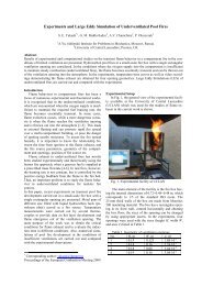
For the present investigation VOLVO
configuration (VR 1) has been considered as
sketched in Fig.1.
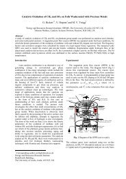
Fig. 1 Bluff body test configuration
It is a bluff body stabilized flame
configuration, and consists of a rectilinear
channel with rectangular cross section,
divided into an inlet section and a
combustion section equipped with a twodimensional
triangular shape flame holder.
The channel is 0.24m width and 0.12m high.
The blockage ratio of the obstacle was 1/3.
The primary intention of this rig is to
investigate phenomena occurring in
afterburners for jet engines.
In the simulations inlet composition assumed
to consist of propane and air, premixed at
equivalence ratio 0.65. For a typical nonreactive
case inlet temperature is 298K,
while for the corresponding reactive case
inlet temperature is 600K. The mass flow
rate into the combustor was 0.60kg/s giving
47500 in the non-reactive case and

Re=24200 in the reactive case. Only the
velocity predictions of reactive case are first
presented in this work. We have used the
120×42×16 grid resolution after the obstacle.
Fig 1 shows the instantaneous velocity
distribution and Fig. 3 shows the mean
velocity distribution. Fig 2 shows the isosurface
velocity plot for velocity equal to 30
m/s. Nevertheless if we include the
combustion phenomena one can expect
smooth velocity field distribution unlike the
present simulation predictions. Due to the
non-availability of the experimental data we
are not able to compare the simulation
results with the experimental data. But
experimental data for the temperature
distribution is available. This data will be
used in the future for the evaluation of the
LES of premixed combustion model. Fig. 1
and Fig. 3 successfully predict the vortexes
after the bluff-body obstacle.
Conclusions
In the present work we have successfully
predicted the velocity distribution for the
bluff body stabilized flame configuration.
Due to the non-availability of the
experimental data we are not able to
compare the simulation results
1)J. Janicka, A. Sadiki., Proc. Comb. Inst: 30
(In Press) (2004)
2)Kerstein, A. R., Ashurst, W., and
Williams, F. A., Phys. Rev. A 37(7):2728–
2731 (1988).
3)Menon, S., and Jou, W. H., Combust. Sci.
Technol. 75:53–72 (1991).
4)Smiljanovski, V., Moser, R. D., and Klein,
R., Combustion Theory and Modelling
1(2):183–215 (1997).
5)Boger, M., Veynante, D., Boughanem, H.,
and Trouve´, A., Proc. Combust. Institute
27:917–926 (1998).
6)Butler, T., and O’Rourke, P., Proc.
Combust. Institute 16:1503–1516 (1977).
7)O’Rourke, P., and Bracco, F. V., J. Comp.
Phys. 33:185–203 (1979).
8)Angelberger, C., Veynante, D.,
Egolfopoulos, F., and Poinsot, T., Annual
Research Briefs 1998, Center for Turbulent
Research, NASA Ames/Stanford University,
Stanford, CA.
9)Colin, O., Ducros, F., Veynante, D., and
Poinsot, T., Phys. Fluids 12(7):1843–1863
(2000).
10)Charlette F., Meneveau C. and Veynante
D., Combustion and Flame 131:159–180
(2002)
11)Germano M., Piomelli U., Moin P., and
Cabot W. H., Phys. Fluids A 3: 1760-1765
(1991)
12)Moin P., Squires K., Cabot W., and Lee
S., Phys. Fluids A 3:2746-2752 (1991)
13)Meneveau C., Lund T. S., and Cabot W.
H., Journal of Fluid Mechanics 319: 353-
385, 1996

Fig.1. Instantaneous velocity vector
distribution
Fig 2. Iso surface (=30 m/sec) velocity
contour
Fig 3.Mean velocity vector distribution