Robust Extended Kalman Filtering in Hybrid Positioning Applications

4th WORKSHOP ON POSITIONING, NAVIGATION AND COMMUNICATION 2007 (WPNC’07), HANNOVER, GERMANY 

Robust Extended Kalman Filtering in Hybrid 

Positioning Applications 

Abstract— The Kalman filter and its extensions has been 

widely studied and applied in positioning, in part because its 

low computational complexity is well suited to small mobile 

devices. While these filters are accurate for problems with 

small nonlinearities and nearly gaussian noise statistics, they 

can perform very badly when these conditions do not prevail. 

In hybrid positioning, large nonlinearities can be caused by the 

geometry and large outliers (blunder measurements) can arise 

due to multipath and non line-of-sight signals. It is therefore of 

interest to find ways to make positioning algorithms based on 

Kalman-type filters more robust. In this paper two methods to 

robustify the Kalman filter are presented. In the first method the 

variances of the measurements are scaled according to weights 

that are calculated for each innovation, thus giving less influence 

to measurements that are regarded as blunder. The second 

method is a bayesian filter that approximates the density of 

the innovation with a non-gaussian density. Weighting functions 

and innovation densities are chosen using Hubers min-max 

approach for the epsilon contaminated normal neighborhood, 

the p-point family, and a heuristic approach. Six robust extended 

Kalman filters together with the classical extended Kalman filter 

(EKF) and the second order extended Kalman filter (EKF2) 

are tested in numerical simulations. The results show that the 

proposed methods outperform EKF and EKF2 in cases where 

there is blunder measurement or considerable linearization errors 

present. 

I. INTRODUCTION 

Algorithms for real time hybrid positioning need to have 

low computational complexity in order to be used in today’s 

mobile devices. Although bayesian filtering provides a theoretically 

complete framework for optimal nonlinear filtering, 

it requires the evaluation of multi-dimensional integrals which 

in general have to be computed using approximate numerical 

techniques such as Monte Carlo. High accuracy can often 

only be achieved with a huge amount of computation time 

and memory. In the linear-gaussian case the integrals can be 

solved analytically and the computation consists only of matrix 

multiplications, sums, etc. The resulting filter, i.e. the Kalman 

filter, has also low memory requirements, because due to the 

gaussianess of the distributions, only the two first moments 

of the distributions need to be stored. Kalman filtering has 

been the subject of extensive study in hybrid positioning 

applications in recent years. Simulations and preliminary test 

results with real data show that the extended Kalman filter 

(EKF) or the second order extended Kalman filter (EKF2) 

might be used in hybrid positioning applications in todays 

mobile devices. 

The Kalman filter is based on the assumption of linear 

1-4244-0871-7/07/$25.00 ©2007 IEEE 

Tommi PERÄLÄ and Robert PICHÉ 

Tampere University of Technology, Finland 

Email: (tommi.perala, robert.piche)@tut.fi 

55 

state and measurement relations and gaussian noise and state 

variables. The noise in the measurements is a combination of 

errors from many different sources and generally does not have 

a gaussian distribution. The performance of the filter may be 

seriously degraded due so-called blunder measurements. This 

kind of corrupted measurements may occur due the physical 

environment e.g. buildings, trees or some geographical obstacles. 

A robust filter should be able to detect the blunder 

measurements and to handle them accordingly. 

One problem in hybrid positioning is that sometimes there 

is hardly enough measurements for a unique position solution 

and discarding a measurement completely might not be an 

option. The motivating question for this paper is practically 

what can one do with the blunder measurements besides 

discarding them. Another problem in hybrid positioning is that 

the measurement functions are non-linear functions of the state 

while the Kalman filter solves a linear filtering problem. Linear 

approximations of the Kalman filter, namely EKF and EKF2 

have been used, but the estimates tend to become biased and 

inconsistent when the linearization errors are large [1]. GPS 

measurements do not have the problem with the non-linearity 

because of the distant location of the satellites. WLAN or 

mobile phone signals however have much smaller range and 

thus the non-linearities can have a significant effect on the 

estimation errors. 

This paper is organized as follows. The next section consists 

of the formulation of the hybrid positioning problem in a 

bayesian framework. The measurement model and the state 

model are described and one approximate solution, namely 

the extended Kalman filter, is given. Section III starts with 

a brief glance at Hubers minimax ideology and two classes 

of densities, the ɛ-contaminated neighbourhood and the ppoint 

family, are defined. Hubers minimax approach is applied 

to these two classes and robust estimators are derived for 

use in robust filter design. A heuristic robust estimator is 

also proposed. Section IV is divided into two distinct parts 

both describing slightly different approaches for robust linear 

filtering. The first approach is to formulate the Kalman filter 

as a deterministic weighted least squares problem and to 

make the filter more robust by proper weighting. The second 

approach is an approximate bayesian filter. Kalman-type filters 

calculate the posterior estimates using the distribution of 

the innovation variable. Approximating the distribution with 

proper non-gaussian distribution should result in more robust 

filter behaviour. Altogether six robust filters are derived. The


results of simulation tests are discussed in section V. 

II. MODEL 

The state of the system at time tk (k =1, 2,...) is modelled 

as a stochastic variable xk. The evolution of the state in time 

is given by a stochastic difference equation 

xk+1 =g k(xk, wk) (1) 

and the initial state x0 is assumed to be normally distributed 

with mean x0 and covariance matrix P0. The measurements 

yk are related to the state by 

yk =hk(xk, vk). (2) 

Here wk describes the noise in the state dynamics and vk 

the noise in the measurements. In this paper the noises are 

assumed to be white zero-mean mutually independent random 

processes, and also independent with the initial state. Let 

y1:k = {yi,i =1,...,k} be the measurements before time 

step tk+1. The measurements used in this work are GPS 

pseudorange measurements and their derivatives, and base 

station range and altitude measurements. Because there is 

unknown clock bias in the satellite measurements, difference 

measurements are used instead. One satellite is chosen as 

reference and all the differences are formed with respect to 

it. Let rk denote the position of the user, rs the position of 

the satellite (basestation) and rs0 the reference satellite. The 

range measurements are 

and the difference measurements 

hk+1(rk+1) =||rs − rk+1|| (3) 

hk+1(rk+1) =||rs − rk+1||−||rs0 − rk+1|| (4) 

The problem now is to solve the conditional probability density 

function (cpdf) of the posterior state, that is the cpdf of 

xk conditioned on y1:k = y1:k. Using the Bayes rule with 

the assumption of white noise sequences the cpdf may be 

formulated as 

p(xk|y1:k) = p(xk|y1:k−1)p(yk|xk) 

(5) 

p(yk|y1:k−1) 

where p(xk|y1:k−1) is the prior density, i.e. the cpdf of xk 

conditioned on y1:k−1 = y1:k−1, p(yk|xk) is the likelihood 

function giving the probability of measurement yk given state 

xk and p(yk|y1:k−1) is the predicted measurement density. 

To derive statistical quantities like mean and covariance from 

cpdf (5) requires integration of numerous multidimensional 

integrals using numerical integration methods. Grid based 

methods and sequential Monte Carlo (particle filter) methods 

have been used succesfully to calculate the posterior estimates. 

They however require a lot of computation and are not suitable 

in real time positioning with todays mobile devices. In the 

next section, one approximate analytic solution, namely the 

extended Kalman filter, is introduced. 

56 

A. Extended Kalman Filter 

The extended Kalman filter is an approximate analytic 

solution to (5) if the noises wk and vk are additive gaussian 

noise sequences. The state and measurement functions are 

linearized according to 

Gk = ∂ g 

k(xk) 

∂xk 

, 

xk=ˆxk 

∂ hk(xk) 

 

 

Hk = 

∂xk xk=ˆx − 

k 

(6) 

where ˆx − 

k and ˆxk are the prior and posterior mean estimates 

at time step tk. The system model becomes 

xk+1 =Gkxk + wk 

yk =Hkxk + vk 

Now the prior density is gaussian with mean and covariance 

given as 

(7) 

(8) 

E(xk|y1:k−1) = ˆx − 

k = Gk ˆxk−1 (9) 

V(xk|y1:k−1) = ˆ P − 

k = Gk ˆ Pk−1G T k +Qk (10) 

where Qk is the covariance of wk. The posterior mean may 

be shown to be 

E(xk|y1:k) =ˆxk =ˆx − 

k + ˆ P − 

k HTk s(yk − Hk ˆx − 

k ) (11) 

where s(yk − Hk ˆx − 

k ) = −∇ ln p(yk|y1:k−1). Denoting the 

covariance of vk with Rk the posterior mean becomes 

ˆxk =ˆx − 

k +Kk(yk − Hk ˆx − 

k 

and the posterior covariance is given by 

ˆPk =(I− KkHk) ˆ P − 

k 

) (12) 

(13) 

where Kk = ˆ P − 

k HT k (Hk ˆ P − 

k HT k +Rk) −1 is the Kalman gain 

matrix. Rk is assumed to be positive definite to make sure that 

the inverse exists. 

III. CLASSES OF DENSITIES 

As seen in the previous section, Kalman filtering is based on 

the assumption of gaussian measurement noise and gaussian 

prior distribution. As argued before, the strict assumption of 

gaussian measurement noise may not be reasonable in hybrid 

positioning applications and therefore some ”more robust” 

densities are presented here. 

Huber [2] proposed a game where Nature choses the distribution 

F ∈ F and the engineer chooses the estimator 

T ∈T, and the asymptotic variance V(T,F) is the pay-off 

to the engineer. The asymptotic variance of an estimator is 

the variance of the estimator when the sample size tends to 

infinity. It can be shown that for certain classes of distributions 

there exists a min-max solution (T0,F0) such that 

min 

T ∈T max 

F ∈F V(T,F)=V(T0,F0) =max 

F ∈F min 

T ∈T V(T,F). 

F0 is called the least favorable distribution of class F and T0 

the min-max robust estimator which is actually the maximum 

likelihood estimator for the least favorable density F0.


A. The ɛ-contaminated normal neighborhood 

Huber [2] considered the case 

contaminated normal neighborhood 

where F is the ɛ- 

Fɛ = {F | F =(1−ɛ)φ + ɛH, 

H continuous symmetrical pdf}, (14) 

where φ is the standard normal probability density and H is a 

continuous symmetrical probability density function. The least 

favorable density for the ɛ-contaminated normal neighborhood 

is 

p 0 

(1−ɛ) 1 

√ − e 2 

ɛ(θ) = 2π θ2, 

|θ|≤ k 

(1−ɛ) 

√ e 

2π 1 

2 k2 (15) 

−k|θ| , |θ|> k 

where the threshold parameter k is given by 

2φ(k) 

ɛ 

− 2Φ(−k) = 

k 1 − ɛ 

(16) 

φ is the standard normal pdf and Φ the standard normal cdf. 

The corresponding min-max robust estimator is based on the 

maximization of the likelihood score of the least favorable 

density, namely 

sH(θ) = ∂ 

∂θ ln p0 

−θ, 

ɛ(θ) = 

−k sign(θ), 

|θ|≤ k 

|θ|> k 

(17) 

Filters using this score function are labelled ”H”. 

B. The p-point family 

Martin and Masreliez [3] assert that if F is the p-point 

family 

−yp 

Fp = {F | F (θ)dθ = p/2 =Φ(−yp), 

−∞ 

F symmetric and continuous at ± yp}, (18) 

where Φ is the standard normal cumulative distribution function, 

then the corresponding least favorable density is given 

by 

p 0 

2 θ K cos ( ), |θ|≤ yp 

2myp 

p(θ) = 

K cos2 ( 1 

2m )e2Kp−1 cos 2 ( 1 

2m )(yp−|θ|) , |θ|> yp 

(19) 

where K =(1−p)(yp(1 + m sin( 1 

m )))−1 and m is given by 

 

2m − p 1+tan 2 

 

1 

1 

2m +tan =0 (20) 

2m 

2m 

The likelihood score of the least favorable density of the ppoint 

family Fp is 

sM(θ) = ∂ 

∂θ ln p0 

1 − myp 

p(θ) = 

tan( θ ), 2myp 

− 

|θ|≤ yp 

1 

C. Estimators without densities 

The min-max robust estimators depend on the shape of 

the least favorable density. However, in more sophisticated 

robust filter design, it might be more appropriate to model the 

score function to correspond to the specific problem instead 

of finding the appropriate contamination classes and the least 

favorable densities. Andrews et. al [4] propose a three-partsredescending 

estimator which is basically a heuristic modification 

of the estimator proposed by Huber. Because redescending 

estimators reject certain measurements a modified version of 

the three-parts-redescending estimator is proposed here. The 

score function is given by 

⎧ 

⎨ θ, |θ|≤ k1 

sD(θ) = k1 sign(θ), k1 < |θ|≤ k2 (22) 

⎩ k1k2 

θ , |θ|> k2 

where the threshold parameters k1 and k2 are chosen to fit the 

problem. In this work k1 is solved as k in (16) and k2 =1.5k1. 

Filters using this score function are labelled ”D”. 

IV. ROBUST KALMAN FILTERING 

In the previous section we have defined some ”robust” 

densities and their corresponding scores. In this section we 

proceed to describe two different ways that these could be 

used to robustify the extended Kalman filter. 

A. Weighted least squares filtering 

The first approach is based on the robust Kalman filtering 

studies of Carosio et. al [5]. The Kalman filter can be shown 

to be equivalent to a deterministic least squares problem 

[6]. The filter is made more robust by replacing the least 

squares score function by the score functions introduced in the 

previous section. By approximating the derivative of the score 

function with a linear approximation the problem is modified 

to a weighted least squares problem, where the weights are 

calculated using the components of the innovation vector and 

a weighting function that corresponds to the selected score 

function. This approach produces filters that give less influence 

to measurements that are classified as blunder. 

The state update equation and the measurement equation of 

the EKF given in (8) may be written as 

 

− 

I 

ˆx 

xk = k 

Gk−1(xk−1 − ˆxk−1)+wk−1 

+ 

Hk yk 

−vk 

(23) 

To make the equations look more simple define 

 

Gk−1(xk−1 − ˆxk−1)+wk−1 

ek = 

(24) 

−vk 

Now 

E(ek) =0, V(ek) =E(eke 

1 tan( myp 2m )sign(θ), 

Filters using this score function are labelled ”M”. 

|θ|> yp 

(21) 

T 

ˆP − 

k )= k 0 

(25) 

0 Rk 

where ˆ P − 

k and Rk are symmetric positive definite and thus 

non-singular. Now define square matrix Mk such that 

M T −1 

ˆP − 

k Mk = k 0 

(26) 

57 

0 Rk


Multiplying (23) by 

Mk and defining 

I 

Nk =Mk , ξk =Mkek, zk =Mk 

Hk 

zk =Nkxk + ξk 

ˆx − 

k 

yk 

 

yields 

(27) 

which is in the form of a standard linear least squares 

regression problem or equivalently 

n 

ˆxk =argmin ((zk)i − (N 

xk 

T k )ixk) 2 

(28) 

i=1 

where (NT k )i is the ith row of Nk. NowE(ξk) =0, 

V(ξk) =E(ξkξT k )=I, and the solution to (28) is given by 

ˆxk =(N T k Nk) −1 N T k zk =ˆx − 

k +Kk(yk − Hk ˆx − 

k 

) (29) 

which will be the posterior mean. The posterior covariance is 

chosen to be 

ˆPk =(N T k Nk) −1 =(I− KkHk) ˆ P − 

k 

(30) 

where Kk = ˆ P − 

k HT k (Hk ˆ P − 

k HT k +Rk) −1 is called the Kalman 

gain matrix. Equations (29) and (30) are of course similar to 

equations (12) and (13). 

Huber [2] introduced a class of estimators, called Mestimators, 

that minimize other functionals than the squares. 

Let ρ(·) denote the functional which will be minimized. Now 

using ρ(·) in (28) in place of (·) 2 gives 

n 

ˆxk =argmin ρ((zk)i − (N 

xk 

T k )ixk) (31) 

i=1 

The minimum is obtained by differentiating the functional to 

be minimized with respect to (xk)j, j=1,...,nx and setting 

these partial derivatives equal to zero. Symbolically this can 

written as nx equations 

n 

(Nk)ijψj((zk)i − (N T k )iˆxk) =0, j =1,...,nx (32) 

i=1 

where ψj =(∇ρ)j and (Nk)ij is the ijth element of matrix 

Nk. The solution of (32) is somewhat difficult to obtain at 

least analytically because the ψ-functions may be non-linear. 

However, (32) can be approximated with a weighted least 

squares problem, namely 

n 

(Nk)ijωk,i((zk)i − (N T k )iˆxk) =0, j =1,...,nx (33) 

i=1 

where the weights ωk,i are given by 

 

ψi((zk)i−(N 

ωk,i = 

T 

k 

)i ˆx− k ) 

(zk)i−(NT k 

)i ˆx− k 

, (zk)i = (NT − 

k )iˆx k 

1, (zk)i =(NT k 

Now the solution of (33) is given by 

)iˆx − 

k 

xk =(N T k ΩkNk) −1 N T k Ωkzk =ˆx − 

k +K∗k(yk − Hk ˆx − 

k 

with covariance 

ˆPk =(I− K ∗ kHk)P ∗ k 

(34) 

) (35) 

(36) 

58 

where K∗ k =P∗ kHT k (R∗ k +HkP∗ kHT k )−1 , 

P∗ k =(ˆ P − 

k )1/2Ω −1 

k−1,1 (ˆ P − 

k )1/2 , R∗ k =R1/2 

k Ω−1 

k−1,2R1/2 k 

 

Ωk,1 0 

Ωk =diag(ωk,1,...,ωk,(nx+ny)) = 

0 Ωk,2 

 

(37) 

where the weights Ωk,1 ∈ R nx×nx and Ωk,2 ∈ R ny×ny . The 

motivation for dividing the weight matrix into two submatrices 

is that the Ωk,1 influences only the state update and Ωk,2 only 

the state correction with measurements. So if robustness is 

desired only in the measurement model one might want to 

define Ωk,1 =I. Depending on the application it might be 

reasonable to use different ψ-function for different components 

in (32). 

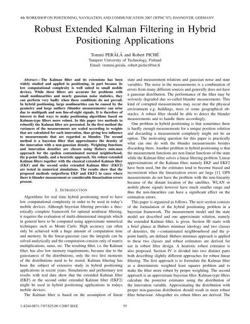
In this paper ψ(·) = −s(·), where the choices for the 

likelihood score s are given in equations (17), (21) and (22). 

Figure 1 shows the ψ-functions and the corresponding weight 

functions. The filters using this method are denoted with prefix 

”WLS”. 

B. Bayesian filtering assuming non-gaussian innovation sequence 

The following method is based on the results of Masreliez 

and Martin [7]. Consider a transformed version of the measurement 

model in (8). 

Tkyk =TkHkxk +Tkvk 

(38) 

The transformation matrix Tk = (Hk ˆ P − 

k HT k +Rk) −1/2 is 

chosen such that TT k Tk =(Hk ˆ P − 

k HT k +Rk) −1 , which is easily 

obtained for example using the singular value decomposition. 

Thus the transformed innovation variable has a standard normal 

density distribution. 

The Kalman filter calculates the posterior state estimates 

using the innovation variable. Under the transformed measurement 

model (38) the posterior mean is given by 

ˆxk =ˆx − 

k + ˆ P − 

k HT k T T k s(nk) (39) 

where the score s(nk) =−∇ ln p(yk|y1:k−1)|yk=nk and 

nk =Tk(yk−Hk ˆx − 

) is the transformed innovation. Masreliez 

k 

and Martin assert that if p(yk|y1:k−1) is the least favorable 

density of either Fɛ or Fp then the posterior mean is given as 

in (39) and the posterior covariance is given by 

ˆPk =(I−KkHk E p(yk|y1:k−1)∇s T 

(yk)|yk=nk ) Pˆ − 

k (40) 

If s = sH or s = sD, then 

E p(yk|y1:k−1)∇s T 

(yk)|yk=nk = 

 

p(yk|y1:k−1)∇s T (yk)|yk=nk dyk =1− 2Φ(k) (41) 

and if s = sM , then 

E p(yk|y1:k−1)∇s T 

(yk)|yk=nk = 

(myp) −2 (1 − p(1 + tan 2 ( 1 

)) (42) 

2m 

The filters using this method are denoted with prefix ”B”


V. TESTING 

The robust methods were implemented in a MATLAB simulation 

test bench for comparison between different filters. The 

simulation test bench was designed to produce dynamic test 

data similar to what could be expected in real-world personal 

positioning scenario. The main difference from the real data is 

that in the simulation the true track and correct measurement 

and motion models are available. The testing process consists 

of first generating a true track of 100 points at one second 

intervals with a velocity-restricted random walk model, then 

generating a set of base station (BS) along the track with 

maximum ranges set so that one to three stations can be heard 

from every point on the track. A GPS constellation is then 

simulated with an elevation mask and shadowing profile set 

so that only a couple of satellites are visible at a time. Finally, 

noisy measurements are generated for each time step from 

the visible satellite ranges and delta-ranges, and base stations 

ranges and altitude measurements. If probability for blunder 

measurement b is greater than zero, then every generated 

measurement fails with a probability of b. 

Several track and measurement sets were generated with different 

measurement sources, measurement noises and blunder 

measurement probabilities. The resulting test bench consists 

of two different sets according to two different choices for 

the blunder measurement probability (0.00 and 0.05). Each 

set has base station and satellite geometries for 9 cases 

representing different difficult positioning situations according 

to the following table 

mean # BS mean # GPS 

Case 1 0.5 0 

Case 2 1.5 0 

Case 3 2.5 0 

Case 4 0.5 2 

Case 5 1.5 2 

Case 6 2.5 2 

Case 7 0 2.5 

Case 8 0 3.5 

Case 9 0 5 

Every case containes 100 tracks, which all have the length of 

100 time steps. 

The test tracks were filtered with the six robust filters of 

this paper, and the mean and covariance of the posterior 

distribution recorded at each time step. The filtered solutions 

were compared to the true track and some statistics derived. 

The filter’s ability to identify blunder measurements was 

also tested and reported. For comparison, the data was also 

processed with EKF and EKF2 [1]. 

A. Results 

The results of the test bench may be seen in tables I and II. 

The quantities calculated are the mean 2D error (MSE) given 

in meters, the bound below which are 95% of the errors, and 

the frequency of inconsistent estimates. A Filter is said to 

be inconsistent if the error estimate is smaller than the actual 

error. For discussion on the consistency of EKF and EKF2 see 

59 

[1]. As expected all the B-filters outperform EKF and EKF2 

in contaminated cases. It is interesting to notice however, 

that when there are GPS measurements available the WLSfilters 

fail compeletely. In basestation only cases the WLSsolvers 

sometimes outperform even the B-filters. The WLS 

filters’ failure seems to be caused by the large innovations that 

sometimes occur with GPS-measurements. The solvers may 

easily give a weight of less than 0.01 for some measurements. 

The filters’ ability to detect the correct corrupted measurement 

was also quite poor. On average the filters identify wrong 

measurement more often than the right measurement, and 

this becomes a serious problem with the WLS-filters, because 

correct measurements get scaled close to zero. All that can 

be said about the blunder detection is, that it is extremely 

hard to tell if a measurement is a blunder measurement by 

measuring the magnitude of the corresponding innovation - 

the prior might also be wrong, but the filter indentifies the 

measurements as blunder. In tables III and IV are listed how 

well the filters detect and identify blunder measurements. The 

actions of the filter may be divided into five categories: 

I Blunder measurements are present and the filter detects 

them correctly. Filter calculates robust estimates. 

II Blunder measurements are present but the filter identifies 

wrong measurement. 

III Blunder measurements are present but the filter does not 

notice it, thus working as EKF. 

IV False alarm. No blunder measurements, but filter calculates 

robust estimates. 

V No blunder measurements and no action. This means that 

the filters, except the filters based on the p-point score, 

work as EKF. 

The frequencies of categories 1-4 are listed in the table 

and the categories are denoted by the corresponding Roman 

numeral. The frequency of category 5 is the frequency of the 

complement of the union of the three first categories. The 

False alarms occur quite often, but they are not very dangerous 

except for WLS-filters with GPS-measurements. If there were 

blunder measurements present, the filters detected them almost 

every time. The most interesting thing however is the huge 

frequency of category 2 in the contaminated case. Because 

the false alarm is the only one from the categories 1-4 which 

can happen in the uncontaminated case, the zero frequencies 

are left out from table III. 

VI. CONCLUSION 

Based on the simulations, the proposed methods seem to 

outperform EKF and EKF2 in contaminated cases and do 

almost as well in normal cases. Therefore, the proposed methods 

should be taken into consideration to be used in mobile 

positioning devices. The approximate bayesian filter is to be 

preferred over the WLS-filter if there are GPS-measurements 

available. WLS-filters might be considered otherwise. The 

score functions should be chosen based on empirical measurement 

data, but without any preliminary knowledge of the 

situation it seems to be safe to use any of the scores proposed 

here. However, the modified Hampel estimator seems to give


best estimates. More sophisticated robust filter should be able 

to indentify certain situations and apply the most convenient 

robust model to them, but this is beyond the scope of this 

paper and left for future study. 

ACKNOWLEDGMENT 

This study was funded by Nokia Corporation. The EKF 

and EKF2 used for reference were implemented by Simo Ali- 

Löytty and the simulation test bench was generated using Niilo 

Sirola’s test bench generator [8]. 

REFERENCES 

[1] S. Ali-Löytty, N. Sirola, and R. Piché, “Consistency of Three Kalman 

Filter Extensions in Hybrid Navigation,” in Proceedings of the European 

Navigation Conference GNSS, July 19-22 2005. 

[2] P. J. Huber, “Robust Estimation of a Location Parameter,” Ann. Math. 

Statis., vol. 35, pp. 73–101, 1964. 

[3] R. D. Martin and C. J. Masreliez, “Robust Estimation via Stochastic 

Approximation,” IEEE Transactions on Information Theory, vol. IT-21, 

no. 3, pp. 263–271, May 1975. 

[4] D. F. Andrews, P. J. Bickel, F. R. Hampel, P. J. Huber, W. H. Rogers, 

andJ.W.Tukey,Robust Estimates of Location: Survey and Advances. 

Princeton University Press, 1972. 

[5] A. Carosio, A. Cina, and M. Piras, “The Robust Statistics Method 

Applied to the Kalman Filter: Theory and Application,” ION GNSS 18th 

International Technical Meeting of the Satellite Division, September 13- 

16 2005. 

[6] A. E. Bryson and Y.-C. Ho, Applied Optimal Control: Optimization, 

Estimation, and Control. Taylor & Francis, 1975. 

[7] C. J. Masreliez and R. D. Martin, “Robust Bayesian Estimation for the 

Linear Model and Robustifying the Kalman Filter,” IEEE Transactions 

on Automatic Control, vol. AC–22, no. 3, pp. 361–371, 1977. 

[8] N. Sirola, S. Ali-Löytty, and R. Piché, “Benchmarking nonlinear filters,” 

in Nonlinear Statistical Signal Processing Workshop NSSPW06, Cambridge, 

September 2006. 

60


−k2 

−k 

−y 

−k1 

ψH(t) 

k 

−k 

ψM(t) 

y 

−y 

ωD(t) 

1 

k 

y 

k1 

k2 

t 

Fig. 1. The ψ- and the ω-functions 

t 

t 

61 

−k2 

−k1 

ψD(t) 

k1 

−k1 

ωH(t) 

1 

−k k 

ωM (t) 

1 

−y y 

k1 

k2 

t 

t 

t


TABLE I 

RESULTS OF THE TESTBENCH WITH BLUNDER PROB. b =0.00 

Case 1 Case 2 Case 3 

b =0% MSE 95% incon MSE 95% incon MSE 95% incon 

EKF 129 490 14.7 40 138 3.8 11 29 0.0 

EKF2 123 453 3.8 45 172 2.2 11 29 0.0 

BHA 138 534 15.3 47 168 4.8 12 30 0.0 

BH 135 510 15.0 43 156 4.5 12 30 0.0 

BM 132 518 14.8 44 152 4.3 12 30 0.0 

WLSHA 144 532 16.0 43 155 4.1 12 31 0.0 

WLSH 132 493 14.9 39 137 3.4 12 30 0.0 

WLSM 133 505 15.3 40 141 3.8 12 30 0.1 


MSE 95% incon MSE 95% incon MSE 95% incon 

EKF 13 33 0.1 9 20 0.0 20 68 0.8 

EKF2 13 33 0.0 9 20 0.0 19 64 0.3 

BHA 13 33 0.1 9 20 0.0 23 76 1.4 

BH 13 34 0.1 9 20 0.0 22 75 1.4 

BM 13 50 0.4 9 20 0.0 21 70 1.2 

WLSHA 13 34 0.1 9 20 0.0 21 71 0.9 

WLSH 13 33 0.1 9 20 0.0 21 70 1.0 

WLSM 13 56 0.2 9 20 0.0 21 70 1.0 


MSE 95% incon MSE 95% incon MSE 95% incon 

EKF 18 41 0.0 19 43 0.0 17 37 0.0 

EKF2 18 41 0.0 19 43 0.0 17 37 0.0 

BHA 19 42 0.0 19 44 0.0 17 38 0.0 

BH 19 42 0.0 19 44 0.0 17 38 0.0 

BM 19 42 0.0 19 44 0.0 17 38 0.0 

WLSHA 19 42 0.0 19 43 0.0 17 37 0.0 

WLSH 19 42 0.0 19 43 0.0 17 37 0.0 

WLSM 19 42 0.0 19 43 0.0 17 38 0.0 

TABLE II 

RESULTS OF THE TESTBENCH WITH BLUNDER PROB. b =0.05 


b =5% MSE 95% incons. MSE 95% incons. MSE 95% incons. 

EKF 351 1466 42.0 168 693 38.6 85 328 35.2 

EKF2 329 1317 37.6 163 667 35.3 84 326 35.0 

BHA 162 656 15.5 89 416 9.7 14 35 0.6 

BH 177 667 18.5 91 433 11.2 15 40 1.1 

BM 193 804 21.1 88 403 12.4 16 42 1.5 

WLSHA 170 725 16.4 90 437 9.0 12 30 0.0 

WLSH 169 667 17.7 83 414 9.3 14 34 0.2 

WLSM 171 653 18.6 79 385 9.5 14 36 0.2 


MSE 95% incons. MSE 95% incons. MSE 95% incons. 

EKF 503 1491 86.5 317 1033 79.2 372 1248 71.6 

EKF2 502 1491 86.5 317 1033 79.2 370 1242 71.1 

BHA 17 42 0.1 12 29 0.5 21 60 0.9 

BH 20 51 0.1 14 36 1.6 32 73 2.6 

BM 21 53 1.6 15 39 2.4 34 82 3.8 

WLSHA 2397 10689 86.0 2150 10283 78.2 4090 19335 72.7 

WLSH 855 1413 84.1 548 1996 75.6 737 2877 68.7 

WLSM 762 2351 84.2 487 1815 75.2 696 2574 68.2 


MSE 95% incons. MSE 95% incons. MSE 95% incons. 

EKF 1020 3065 92.3 989 2705 93.8 949 2548 95.5 

EKF2 1020 3065 92.3 989 2705 93.8 949 2548 95.5 

BHA 25 59 0.3 23 49 0.0 21 45 0.0 

BH 28 68 0.4 26 56 0.3 26 57 1.0 

BM 30 73 0.9 27 60 0.8 28 61 2.1 

WLSHA 7090 25138 90.5 6787 26024 92.5 3839 15123 94.2 

WLSH 2351 7926 90.7 2013 6255 93.0 1734 5530 94.8 

WLSM 2283 7617 90.4 1873 6032 93.1 1615 4936 94.9 

62


TABLE III 

BLUNDER DETECTION WITH BLUNDER PROBABILITY b =0.00 

Case 1 Case 2 Case 3 Case 4 Case 5 Case 6 Case 7 Case 8 Case 9 

b =0% III III III III III III III III III 

BHA 0.21 0.28 0.37 0.45 0.55 0.33 0.30 0.41 0.59 

BH 0.21 0.27 0.37 0.45 0.55 0.33 0.30 0.41 0.59 

BM 0.22 0.29 0.39 0.46 0.56 0.34 0.30 0.41 0.59 

WLSHA 0.38 0.43 0.52 0.58 0.66 0.47 0.46 0.57 0.70 

WLSH 0.37 0.42 0.51 0.58 0.66 0.47 0.46 0.57 0.70 

WLSM 0.37 0.42 0.51 0.58 0.66 0.47 0.47 0.57 0.70 

TABLE IV 

BLUNDER DETECTION WITH BLUNDER PROBABILITY b =0.05 


b =5% I II III IV I II III IV I II III IV 

BHA 0.01 0.03 0.02 0.25 0.02 0.04 0.02 0.30 0.03 0.06 0.03 0.41 

BH 0.01 0.03 0.01 0.27 0.02 0.04 0.02 0.32 0.03 0.06 0.02 0.44 

BM 0.01 0.03 0.01 0.29 0.02 0.04 0.02 0.34 0.03 0.06 0.02 0.45 

WLSHA 0.02 0.02 0.01 0.40 0.03 0.03 0.01 0.42 0.03 0.06 0.02 0.50 

WLSH 0.02 0.02 0.01 0.42 0.03 0.03 0.01 0.44 0.03 0.06 0.02 0.52 

WLSM 0.02 0.02 0.01 0.42 0.03 0.03 0.01 0.44 0.03 0.06 0.02 0.52 


I II III IV I II III IV I II III IV 

BHA 0.07 0.11 0.09 0.45 0.09 0.16 0.09 0.47 0.05 0.08 0.09 0.39 

BH 0.08 0.11 0.09 0.46 0.09 0.17 0.08 0.48 0.05 0.08 0.08 0.41 

BM 0.08 0.11 0.09 0.47 0.09 0.17 0.08 0.49 0.05 0.08 0.08 0.42 

WLSHA 0.22 0.05 0.00 0.70 0.25 0.08 0.01 0.65 0.15 0.04 0.01 0.69 

WLSH 0.22 0.05 0.01 0.69 0.24 0.08 0.01 0.64 0.15 0.05 0.01 0.68 

WLSM 0.22 0.06 0.00 0.70 0.23 0.09 0.01 0.64 0.15 0.05 0.01 0.67 


I II III IV I II III IV I II III IV 

BHA 0.08 0.14 0.03 0.27 0.10 0.19 0.02 0.31 0.16 0.25 0.01 0.37 

BH 0.08 0.14 0.02 0.29 0.11 0.18 0.02 0.33 0.16 0.25 0.01 0.39 

BM 0.08 0.14 0.02 0.30 0.10 0.19 0.02 0.34 0.16 0.25 0.01 0.40 

WLSHA 0.24 0.01 0.00 0.72 0.30 0.01 0.00 0.67 0.41 0.01 0.00 0.57 

WLSH 0.24 0.01 0.00 0.72 0.30 0.01 0.00 0.67 0.41 0.01 0.00 0.57 

WLSM 0.24 0.01 0.00 0.71 0.30 0.01 0.00 0.67 0.41 0.01 0.00 0.57 

63

Robust Extended Kalman Filtering in Hybrid Positioning Applications

Create successful ePaper yourself

Delete template?

Save as template?