A Motion Model for Articulated Vehicles and a Distributed ...

AMotionModelforArticulatedVehiclesanda
Distributed Acceleration Measurement System
Abstract—A motion model is developed for a trailer-truck
combination that fuses the differential equations governing the
motion of the trailer with the dynamics model of the truck. Three
different parametrisations of the vehicle state are proposed. The
resulting model is a stepping stone for a filtering solution for
tracking the position and attitude of articulated vehicles, such
as trailer-trucks, articulated buses or work machines, or even
trains.
Niilo Sirola and Jarkko Rouhe
I. INTRODUCTION
FOR vehicle positioning and tracking, it is often convenient
to model the vehicle as a singular point and compute
its position, velocity, or other quantities of interest. When
building positioning or tracking systems for articulated vehicles,
such as trailer-trucks, articulated buses, work machines or
trains for example, it may be advantageous to model some the
vehicle as a system of connected bodies instead of abstracting
it as a single point. Additionally, in our application the sensors
are not attached to a single rigid body but to different parts
of the vehicle, so that it is necessary to solve for the attitude
of the vehicle in order to fuse the measurements. It would
also be possible to refine the models all the way to tires and
suspension, but this level of detail is not necessary here.
The motion of trailer-trucks, or articulated vehicles in general,
has been studied for the purposes of building automated
vehicle control systems and driver assistance devices [1].
There are some theoretical papers modelling the motion of an
idealized articulated vehicle for e.g. studying jack-knifing [2]
or deriving rules-of-thumb for road design [3]. Often, the goal
of modelling is to build some control system for the vehicle,
such as in [4] or [5].
This study aims at tracking the motion and behaviour of
a trailer-truck by using several accelerometers installed in
different parts of the vehicle. We present a dynamics model
for a trailer-truck in a form that is applicable in nonlinear
filtering using Extended Kalman filter of Particle filters. To our
knowledge there are no articulated vehicle models applicable
to filtering presented in the literature so far.
II. RAW DATA
Test data was collected from a fuel trailer-truck driving its
normal scheduled route in July-August 2009. The trailer-truck
(hereafter referred to as the vehicle) was equipped with four
independent sensor packs, one of which was a gps receiver
N. Sirola was with Department of Mathematics, Tampere University of
Technology, Finland. He is now with Taipale Telematics, PO Box 42, 33901
Tampere, Finland (e-mail: niilo.sirola@taipaletelematics.com)
J. Rouhe is with Taipale Telematics, Finland.
Manuscript received December 1, 2009; revised March 16, 2010.
fixed inside the cab, and the rest three were standalone batterypowered
3D accelerometer packs (Taipale Telematics Sensior),
one fixed rigidly to the side of the truck and two to the trailer.
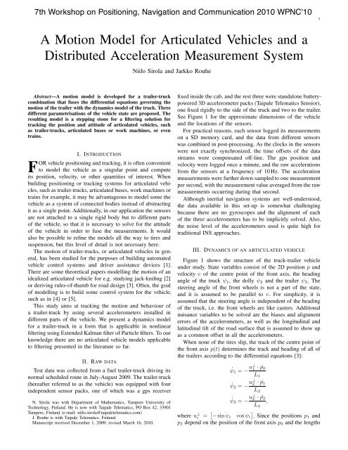
See Figure 1 for the approximate dimensions of the vehicle
and the locations of the sensors.
For practical reasons, each sensor logged its measurements
on a SD memory card, and the data from different sensors
was combined in post-processing. As the clocks in the sensors
were not exactly synchronized, the time offsets of the data
streams were compensated off-line. The gps position and
velocity were logged once a minute, and the raw accelerations
from the sensors at a frequency of 10 Hz. The acceleration
measurements were further down-sampled to one measurement
per second, with the measurement value averaged from the raw
measurements occurring during that second.
Although inertial navigation systems are well-understood,
the data available in this set-up is somewhat challenging
because there are no gyroscopes and the alignment of each
of the three accelerometers has to be implicitly solved. Also,
the noise level of the accelerometers used is quite high for
traditional INS approaches.
III. DYNAMICS OF AN ARTICULATED VEHICLE
Figure 1 shows the structure of the truck-trailer vehicle
under study. State variables consist of the 2D position p and
velocity v of the centre point of the front axis, the heading
angle of the truck ψ1, thedollyψ2 and the trailer ψ3. The
steering angle of the front wheels is not a part of the state,
and it is assumed to be parallel to v. For simplicity, it is
assumed that the steering angle is independent of the heading
of the truck, i.e. the front wheels are like casters. Additional
nuisance variables to be solved are the biases and alignment
errors of the accelerometers, as well as the longitudinal and
latitudinal tilt of the road surface that is assumed to show up
as a common offset in all the accelerometers.
When none of the tires slip, the track of the centre point of
the front axis p(t) determines the track and heading of all of
the trailers according to the differential equations [3]:
˙ψ1 = − u⊥ 1
˙ψ2 = − u⊥ 2
˙ψ3 = − u⊥ 3
L1
L2
· ˙ p0
· ˙ p1
where u ⊥ i = − sin ψi cos ψi
.Sincethepositionsp1 and
p2 depend on the position of the front axis p0 and the lengths
L3
· ˙
p2
,
1

s3
B3
p3
W
u3
ψ3
Fig. 1. The truck, dolly and semitrailer under study, with the locationsofthesensorunits.
L3
and angles of connecting structures, we can write
˙ψ1 = − u⊥ 1
L1
· ˙p0
˙ψ2 = − u⊥ 2 · (˙p0 + B1 ˙ ψ1u ⊥ 1 )
L2
˙ψ3 = − u⊥ 3 · (˙p0 + B1 ˙ ψ1u ⊥ 1 + B2 ˙ ψ2u ⊥ 2 )
This model gives a constraint that the motion of the front axis
of the vehicle and the positions and headings of all the moving
parts have to satisfy. Unfortunately, the relationship is through
asystemofdifferentialequationsthatdonothaveananalytic
solution, so it is not trivial to implement.
There are three different approaches to implement the
constraint:
1) Choose the variables such that they are independent, and
represent the dependent variables as functions of independent
variables. This will however lead to very complicated
measurement models for the sensors mounted
in the trailer.
2) Use the equation as a constraint and enforce it between
iterations. This has the drawback of requiring that ψi
˙
are included as variables, which increases the state
dimension and requires a dynamics model for them as
well.
3) Use the propagation equation directly in the dynamics
model. Then ψi will be variables but their derivatives
need not be. The time propagation step is then done
through solving the differential equation system for one
step. This approach shows most promise for subsequent
filtering applications.
Depending on the parametrisation and the choice of nuisance
parameters, the state dimension is of the order of 20–
30. The resulting filtering problem is very challenging for
nonlinear filters, because of the high state dimension, and
additionally both the dynamics model and measurement model
are very nonlinear and computation-intensive.
L3
.
s2
p2
B2
(1)
ψ2
u2
L2
p1
B1
ψ1
u1
L1
s1
p0
IV. MOTION MODEL
In this work, the state xk and the measurements yk of the
vehicle are assumed to follow the models
xk+1 = fk(xk,wk)
yk = hk(xk)+vk
where the former is called the dynamics model and the latter
the measurement model. Thestochasticnoisetermsvkand wk
are assumed white, zero-mean, and independent of each other
and of the initial state x0. Thispaperconcentratesonfinding
an applicable and tractable form for fk.
In continuous form, the dynamics model can be written as
⎡ ⎤ ⎡ ⎤
p0 ˙p0
⎢ ˙p0 ⎥ ⎢ ¨p0 ⎥
⎢ ⎥ ⎢ ⎥
˙x = ∂
∂t
= f(t, x)
˙p0
⎢ ¨p0 ⎥ ⎢g(t,
x) ⎥
⎢ ⎥ ⎢ ⎥
⎢
⎢ψ1⎥
⎢ ψ1
˙ ⎥
⎥ ⎢ ⎥
⎢ψ2⎥
⎢ ⎥ = ⎢ ψ2
˙ ⎥
⎢ψ3⎥
⎢
⎢ ⎥ ⎢
˙ ⎥ ψ3 ⎥
⎢ φ ⎥ ⎢
⎥ ⎢ 0 ⎥
⎣ θ ⎦ ⎣ 0 ⎦
b 0
where the function g(t, x) is used to inject the steering
behaviour of the truck. One example would be g(t, x) =
(u1 · ˙p0) ˙ ψ1
The time propagation relations can be written as [6]
˙x(t) =f(x(t),t)
˙
P (t) =F [t; x(t)]P (t)+P (t)F T [t; x(t)] + GQG T
where F = ∂
∂x f(x, t). Thetimeupdatestepcanbesolved
from this with numerical differential equation solvers methods.
Let the state vector be
V. MEASUREMENT MODEL
x = p0, ˙p0, ¨p0, ψ1, ψ2, ψ3, ˙
ψ1, ˙
ψ2, ˙
ψ3, φ, θ, b ,
where φ is the rotation of the vehicle around the x axis (roll)
and θ around the y axis (pitch), which depend on the slope
2
(2)

g
g
g
0.2
0.1
0
−0.1
−0.2
0.2
0
−0.2
0.2
0.1
0
−0.1
−0.2
along−track acceleration
12:34 12:35
cross−track acceleration
truck trailer front trailer rear
12:34 12:35
vertical acceleration
12:34 12:35
Fig. 2. Accelerations at the different sensors during three minutes. The vehicle starts from rest at a traffic light, makes atightrightturnandacceleratesto
about 60 km/h. After 12:34 starts a ramp to a motorway that curves to the right.
of the road and are assumed constant in both the truck and
trailer. The state vector additionally contains the biases b of
each accelerometer axis, a total of 9 additional variables in
this case.
The attitude of the first accelerometer is C(ψ1), thus it
measures
a1 = C(ψ1) T (¨s1 + g)+b1.
Note that the sensor logic automatically adds one g to the z
axis measurement to compensate for the normal force when
the sensor is level, i.e. 0=φ = θ. Thishoweveraddsbiasto
measurements whenever the sensor is tilted. Here we used the
shorthand g = 0 0 g T .
Expanding the second derivative of the sensor position for
each sensor(see Appendix 1 for details), the measurement
models for the three sensors are
a1 = C(ψ1) T ¨p0 + ˙
2
ψ1 I2C(ψ1)q1 + g + b1 + v1
a2 = C(ψ3) T ¨p0 + B1 ˙
2
ψ1 I2C(ψ1)u1
+ B2 ˙
2
ψ2 I2C(ψ2)u2 − ˙
2
ψ3 I2C(ψ3)q2 + g + b2 + v2
a3 = C(ψ3) T ¨p0 + B1 ˙
2
ψ1 I2C(ψ1)u1
+ B2 ˙
2
ψ2 I2C(ψ2)u2 − ˙
2
ψ3 I2C(ψ3)q3 + g + b3 + v3.
(3)
The gps position and velocity measurements can be written
simply as
pgps = p0 + v4
vgps =˙p0 + v5.
(4)
Note that the gps receiver has already applied some kind of
smoothing or filter to the position and velocity outputs, so any
additional processing has to be done with care.
Figure 2 shows the accelerations measured at the three
sensors during a short interval of normal driving.
VI. CONCLUSIONS
This paper presents some initial work on building a comprehensive
model for tracking and estimating the attitude of an
articulated truck. The differential equations that form the basis
of the motion model are presented, and measurement equations
for accelerometers fixed into arbitrary positions within the
vehicle combination were derived.
The current problem is very challenging for nonlinear filters,
because the dimension of the state, 26, is fairly high, and both
the dynamics and measurement models are very nonlinear and
computation-intensive. As for the subsequent filter implementation,
the Unscented Kalman Filter (UKF) [7] is a promising
alternative, because it does not require the derivatives of the
models to be computed, and works with a moderate number
of function evaluations compared to particle filters.
ACKNOWLEDGEMENTS
Niilo Sirola was funded by the Academy of Finland.
A. Measurement model
APPENDIX
Each sensor measures the net acceleration at its position in
the sensor coordinates. Each sensor is assumed to be perfectly
3

lined up within the body it is connected to. The acceleration
measurement at ith sensor is
ai = C(ψ) T (¨si + g)+bi, (5)
where C(ψ) =R(ψ, φ, θ) is the rotation matrix, and the roll
and pitch angles φ and θ are assumed constant.
The measurement depends on the accelerations at the sensor
coordinates s1, s2,ands3,whichcanbewrittenintermsofthe
coordinates of the front axis and the angles and lengths in the
system. Referring to Figure 1 and denote the relative position
of a sensor in the coordinates of the part of the vehicle it is
attached to with qi, theabsolutepositionsofthesensorsare
s1 = p0 + C(ψ1)q1
s2 = p0 − C(ψ1)B1u1 − C(ψ2)B2u2 + C(ψ3)q2
s3 = p0 − C(ψ1)B1u1 − C(ψ2)B2u2 + C(ψ3)q3
Then, assuming the angle velocities are constant, that is,
¨ψi =0,weget
¨s1 =¨p0 + ˙
2 ′′
ψ1 C (ψ1)q1
¨s2 =¨p0 − B1 ˙
2 ′′
ψ1 C (ψ1)u1
− B2 ˙
2 ′′
ψ2 C (ψ2)u2 + ˙
2 ′′
ψ3 C (ψ3)q2
¨s3 =¨p0 − B1 ˙
2 ′′
ψ1 C (ψ1)u1
− B2 ˙
2 ′′
ψ2 C (ψ2)u2 + ˙
2 ′′
ψ3 C (ψ3)q3
Note that we can simplify the second derivatives of the
rotation matrices a bit by noting that
⎡
⎤
cos ψ − sin ψ 0
C(ψ) = ⎣sin ψ cos ψ 0⎦
R(0, φ, θ)
0
C
0 1
′′ ⎡
− cos ψ
(ψ) = ⎣− sin ψ
sin ψ
− cos ψ
⎤
0
0⎦
R(0, φ, θ)
0
⎡
1
= − ⎣0 0
1
0 0
⎤
0
0⎦C(ψ)
=−I2C(ψ)
0 0 0
Thus, substituting to Eq. (5), the measurements at each
sensor are
a1 = C(ψ1) T ¨p0 + ˙
2
ψ1 I2C(ψ1)q1 + g + b1
a2 = C(ψ3) T ¨p0 + B1 ˙
2
ψ1 I2C(ψ1)u1
+ B2 ˙
2
ψ2 I2C(ψ2)u2 − ˙
2
ψ3 I2C(ψ3)q2 + g + b2
a3 = C(ψ3) T ¨p0 + B1 ˙
2
ψ1 I2C(ψ1)u1
+ B2 ˙
2
ψ2 I2C(ψ2)u2 − ˙
2
ψ3 I2C(ψ3)q3 + g + b3
These formulae may be simplified further, but it would make
it harder to modify them if the sensor configuration changes.
REFERENCES
[1] C. Chen and M. Tomizuka, “Dynamic modling of articulated vehicles for
automated highway systems,” in Proceedings of the American Control
Conference, Seattle,Washington,June1995,pp.653–657.
[2] T. V. Fossum and G. N. Lewis, “A mathematical model for trailer-truck
jackknifing,” SIAM Review, vol. 23, no. 1, pp. 95–99, 1981. [Online].
Available: http://www.jstor.org/stable/2029841
[3] G. E. Prince and S. P. Dubois, “Mathematical models for motion of the
rear ends of vehicles,” Mathematical and Computer Modelling, vol.49,
no. 9-10, pp. 2049–2060, May 2009.
[4] M. Sampei, T. Tamura, T. Kobayashi, and N. Shibui, “Arbitrary path
tracking control of articulated vehicles using nonlinear control theory,”
IEEE Transactions on Control Systems Technology, vol.3,no.1,pp.125–
131, 1995.
[5] C. Chen and M. Tomizuka, “Modeling and control of articulated vehicles,”
University of California, Berkeley, California PATH Research Report
UCB-ITS-PRR-97-42, 1997.
[6] P. S. Maybeck, Stochastic models, estimation and control, Volume 2.
Academic Press, 1982.
[7] S. Särkkä, “On unscented Kalman filtering for state estimation of
continuous-time nonlinear systems,” IEEE Transactions on Automatic
Control, vol.52,no.9,pp.1631–1641,September2007.
4