1 Analysis of Point (Event) Data II Describing the Spatial ... - Capita
1 Analysis of Point (Event) Data II Describing the Spatial ... - Capita
1 Analysis of Point (Event) Data II Describing the Spatial ... - Capita

Create successful ePaper yourself
Turn your PDF publications into a flip-book with our unique Google optimized e-Paper software.
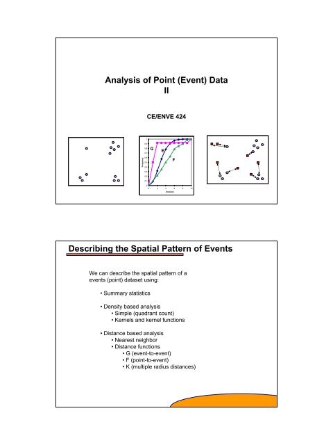
<strong>Analysis</strong> <strong>of</strong> <strong>Point</strong> (<strong>Event</strong>) <strong>Data</strong><br />
<strong>II</strong><br />
Frequency<br />
1<br />
0.9<br />
0.8<br />
0.7<br />
0.6<br />
0.5<br />
CE/ENVE 424<br />
G<br />
E<br />
F<br />
0.4<br />
0.3<br />
0.2<br />
0.1<br />
0<br />
0 2 4 6 8 10<br />
Distance<br />
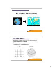
<strong>Describing</strong> <strong>the</strong> <strong>Spatial</strong> Pattern <strong>of</strong> <strong>Event</strong>s<br />
We can describe <strong>the</strong> spatial pattern <strong>of</strong> a<br />
events (point) dataset using:<br />
• Summary statistics<br />
• Density based analysis<br />
• Simple (quadrant count)<br />
• Kernels and kernel functions<br />
• Distance based analysis<br />
• Nearest neighbor<br />
• Distance functions<br />
• G (event-to-event)<br />
• F (point-to-event)<br />
• K (multiple radius distances)
Relating Intensity Patterns<br />
The intensity patterns derived using <strong>the</strong> methods previously discussed provide<br />
a meaningful analysis endpoint, particularly when comparing patterns among<br />
data sets<br />
However, we’re frequently interested in more explicit methods for describing <strong>the</strong><br />
a point spatial pattern<br />
The most common approach is to test against complete spatial<br />
randomness (CSR):<br />
• Is <strong>the</strong> event pattern significantly more clustered than what<br />
would be expected from a random distribution?<br />
• Is <strong>the</strong> event pattern more uniformly spaced than would be<br />
expected from a random distribution?<br />
Complete <strong>Spatial</strong> Randomness<br />
A process is considered random if its intensity (average<br />
number <strong>of</strong> events per unit area) is constant over <strong>the</strong> region<br />
<strong>of</strong> interest.<br />
1) <strong>the</strong> chance <strong>of</strong> a given x,y point existing is equal to <strong>the</strong><br />
chance any o<strong>the</strong>r point existing (uniform probability<br />
distribution)<br />
2) <strong>the</strong> existence <strong>of</strong> a x,y point is independent <strong>of</strong> <strong>the</strong><br />
existence <strong>of</strong> any o<strong>the</strong>r point<br />
These two conditions constitute an independent random<br />
process (IRP) or complete spatial randomness (CSR)
Complete <strong>Spatial</strong> Randomness<br />
CSR is a baseline hypo<strong>the</strong>sis (null hypo<strong>the</strong>sis) against which is assessed<br />
whe<strong>the</strong>r an observed pattern is evenly spaced, clustered, or random.<br />
In testing for CSR, we define a model for CSR. We could simulate a <strong>the</strong><br />
pattern for number <strong>of</strong> events over a region <strong>of</strong> interest using <strong>the</strong> model. We<br />
can <strong>the</strong>n compare <strong>the</strong> spatial distribution <strong>of</strong> <strong>the</strong> modeled patterns with our<br />
observed pattern.<br />
The standard model to use in testing spatial point patterns follow a Poisson<br />
distribution.<br />
The probability <strong>of</strong> observing k events in one unit area in our region is<br />
approximated by:<br />
6<br />
k<br />
λ<br />
λ<br />
Mean = Variance<br />
5<br />
−<br />
P(<br />
k)<br />
=<br />
Quadrant Count<br />
e<br />
k!<br />
n<br />
λ = e ≈ 2.<br />
718<br />
a<br />
So <strong>the</strong> ratio <strong>of</strong><br />
mean/variance can<br />
be used to<br />
determine if <strong>the</strong><br />
pattern is random<br />
Frequency<br />
4<br />
3<br />
2<br />
1<br />
0<br />
1 2 3 4 5 6 7<br />
Bin<br />
Recall from <strong>the</strong> last lecture, a quadrant count is conducted by superimposing a<br />
regular grid over data, counting <strong>the</strong> number <strong>of</strong> events in each grid cell and divide<br />
<strong>the</strong> count by its cell area to get intensity.<br />
47 grid cells<br />
Mean cell count<br />
47<br />
µ = = 1.<br />
175<br />
40<br />
variance<br />
mean<br />
=<br />
Variance:<br />
1 ∑=<br />
n<br />
2<br />
s = µ<br />
n i 1<br />
85.<br />
775<br />
= =<br />
40<br />
2.<br />
1444<br />
1.<br />
175<br />
=<br />
1.<br />
825<br />
( ) 2<br />
k −<br />
2.<br />
1444<br />
A s 2 to µ ratio greater than 1 indicates<br />
clustering
Nearest Neighbor<br />
7<br />
The expected value <strong>of</strong> mean nearest neighbor is: E(<br />
d )<br />
1<br />
9<br />
8<br />
20<br />
4<br />
3<br />
5<br />
2<br />
6<br />
11<br />
10<br />
12<br />
event<br />
nearest<br />
neighbor dmin<br />
1 3 10<br />
2 5 2<br />
3 5 1<br />
4 3 1.5<br />
5 3 1<br />
6 5 1.5<br />
7 8 1<br />
8 7 1<br />
9 7 2<br />
10 11 1<br />
11 10 1<br />
12 10 1.5<br />
G Function<br />
20<br />
The G Function provides a<br />
cumulative frequency<br />
distribution <strong>of</strong> <strong>the</strong> nearest<br />
neighbor event-event distances<br />
7<br />
1<br />
9<br />
8<br />
. [ d ( s ) d]<br />
no min i <<br />
G( d ) =<br />
n<br />
4<br />
3<br />
5<br />
2<br />
6<br />
11<br />
10<br />
12<br />
Frequency<br />
1<br />
0.9<br />
0.8<br />
0.7<br />
0.6<br />
0.5<br />
0.4<br />
0.3<br />
0.2<br />
0.1<br />
d<br />
n<br />
∑<br />
i=<br />
= 1<br />
min<br />
d<br />
24 . 5<br />
= =<br />
12<br />
min<br />
n<br />
( s )<br />
2.<br />
04<br />
i<br />
1<br />
=<br />
2 λ<br />
Calculating <strong>the</strong> ratio <strong>of</strong> our observed mean<br />
nearest neighbor distance and <strong>the</strong> expected<br />
distance provides a measure <strong>of</strong> clustering<br />
E<br />
0<br />
0 2 4 6 8 10<br />
Distance<br />
dmin<br />
R =<br />
1/<br />
2<br />
R =<br />
[ G(<br />
d ) ]<br />
0.<br />
5<br />
λ<br />
2.<br />
04<br />
= 0.<br />
71<br />
12 /( 20X<br />
20)<br />
A ratio less than 1<br />
indicates clustering<br />
CSR Expected G(d):<br />
= 1−<br />
e<br />
−λπd<br />
Distance G(d) Count G(d) Freq. E(G) Freq E(G) Count<br />
0 0 0.000 0.000 0.000<br />
1 6 0.500 0.090 1.079<br />
2 5 0.917 0.314 2.690<br />
3 0 0.917 0.572 3.093<br />
4 0 0.917 0.779 2.482<br />
5 0 0.917 0.905 1.519<br />
6 0 0.917 0.966 0.734<br />
7 0 0.917 0.990 0.285<br />
8 0 0.917 0.998 0.090<br />
9 0 0.917 1.000 0.023<br />
10 1 1.000 1.000 0.005<br />
2
F Function<br />
The F Function provides a<br />
cumulative frequency<br />
distribution <strong>of</strong> <strong>the</strong> nearest<br />
neighbor point-event distances<br />
7<br />
1<br />
9<br />
8<br />
. [ dmin<br />
( p , S ) d ]<br />
no<br />
i <<br />
F( d ) =<br />
m<br />
K Function<br />
n<br />
λ =<br />
a<br />
4<br />
3<br />
5<br />
2<br />
6<br />
11<br />
10<br />
12<br />
Frequency<br />
CSR Expected F(d):<br />
1<br />
0.9<br />
0.8<br />
0.7<br />
0.6<br />
0.5<br />
0.4<br />
0.3<br />
0.2<br />
0.1<br />
E<br />
[ F(<br />
d ) ]<br />
G E<br />
= 1−<br />
e<br />
F<br />
0<br />
0 2 4 6 8 10<br />
Distance<br />
−λπd<br />
The K function uses all distances between events and provides a measure<br />
<strong>of</strong> spatial dependence over a wider range <strong>of</strong> scales.<br />
K(<br />
d)<br />
n<br />
∑<br />
i=<br />
= 1<br />
no<br />
. [ S ∈C(<br />
s , d ) ]<br />
nλ<br />
i<br />
[ K(<br />
d ) ]<br />
E =<br />
λπ 2<br />
d<br />
λ<br />
2<br />
= πd<br />
( d )<br />
d<br />
K<br />
L( d ) = −<br />
π<br />
2
L Function<br />
7<br />
1<br />
9<br />
8<br />
4<br />
3<br />
5<br />
2<br />
6<br />
11<br />
10<br />
12<br />
Distance K(d) L(d) E(K(d)) E(L(d))<br />
0 0.000 0.000 0.000 0<br />
1 16.667 1.303 3.142 0<br />
2 30.556 1.119 12.566 0<br />
3 30.556 0.119 28.274 0<br />
4 30.556 -0.881 50.265 0<br />
5 30.556 -1.881 78.540 0<br />
6 30.556 -2.881 113.097 0<br />
7 30.556 -3.881 153.938 0<br />
8 30.556 -4.881 201.062 0<br />
9 30.556 -5.881 254.469 0<br />
10 33.333 -6.743 314.159 0<br />
Multi Variant <strong>Analysis</strong><br />
An L(d) <strong>of</strong> 0 is expected<br />
An L(d) above <strong>the</strong> “zero line” indicates <strong>the</strong>re are<br />
more events at that separation distance than<br />
expected<br />
An L(d) below <strong>the</strong> “zero line” indicates <strong>the</strong>re are<br />
fewer events at that separation distance than<br />
expected<br />
Sometimes you have multiple data sets and wish to know if <strong>the</strong><br />
spatial patterns among <strong>the</strong>m are similar.<br />
Cross functions are variants on <strong>the</strong> previously discussed<br />
distance-based analysis methods.<br />
2<br />
1<br />
0<br />
0 2 4 6 8 10<br />
-1<br />
For G(d), <strong>the</strong> distance <strong>of</strong> interest is between events in one dataset<br />
and events in ano<strong>the</strong>r dataset<br />
For K(d), counts <strong>the</strong> number <strong>of</strong> events one dataset based on<br />
distances from events in ano<strong>the</strong>r dataset<br />
L(d)<br />
-2<br />
-3<br />
-4<br />
-5<br />
-6<br />
-7<br />
Distance
Incorporating Temporal Dimension<br />
Intensity is defined as <strong>the</strong> number <strong>of</strong> events per unit area in unit time<br />
Are events clustered in space and time?<br />
Distance is a statistical distance in units <strong>of</strong> physical distance X time<br />
distance.<br />
One method for determining whe<strong>the</strong>r <strong>the</strong>re is space-time dependence<br />
is to calculate<br />
1) a K(d,t) for space*time distance<br />
2) a K(d) and K(t) separately<br />
3) K(d) * K(t)<br />
4) K(d,t) – K(d)*K(t)<br />
Examples<br />
Phytopathology Vol. 92, No. 4, 2002 361-377<br />
Background<br />
Florida has been substantially impacted by Asiatic citrus canker, a disease<br />
that can cause defoliation, dieback and fruit drop<br />
Objectives<br />
Does removing healthy citrus trees within a 38 m radius <strong>of</strong> infected trees<br />
curtail fur<strong>the</strong>r spread <strong>of</strong> <strong>the</strong> disease<br />
Methods Used<br />
K function for testing complete spatial randomness (CSR)
American Journal <strong>of</strong> Tropical Medicine and Hygiene Vol. 58, No 3, 1998 287-298<br />
Background<br />
Dengue fever, a viral disease transmitted by mosquitoes, can spread<br />
rapidly and is without a vaccine. Cases tend to be clustered because it is assumed<br />
that female mosquitoes rarely travel fur<strong>the</strong>r than 50-100 m in <strong>the</strong>ir lifetime.<br />
Objectives<br />
What is <strong>the</strong> spatial-temporal pattern <strong>of</strong> <strong>the</strong> diesease<br />
Methods Used<br />
K function for testing complete spatial randomness (CSR)
Projects and Articles<br />
Begin searching for articles to get ideas<br />
Also try to understand <strong>the</strong> availability <strong>of</strong> data<br />
This weekend, <strong>the</strong> class website will be updated with data sources, links<br />
to online journals, references to o<strong>the</strong>r journals<br />
If you come across a good resource, please let me know and I’ll add it to<br />
<strong>the</strong> website