Relativistic Astrophysics and compact objects - Dipartimento di ...
Relativistic Astrophysics and compact objects - Dipartimento di ...
Relativistic Astrophysics and compact objects - Dipartimento di ...

You also want an ePaper? Increase the reach of your titles
YUMPU automatically turns print PDFs into web optimized ePapers that Google loves.
<strong>Relativistic</strong> <strong>Astrophysics</strong> <strong>and</strong> <strong>compact</strong> <strong>objects</strong><br />
Luca Del Zanna<br />
<strong>Dipartimento</strong> <strong>di</strong> Fisica e Astronomia, Università degli Stu<strong>di</strong> <strong>di</strong> Firenze<br />
luca.delzanna@unifi.it<br />
Part of the course Astrofisica delle alte energie,<br />
Laurea Magistrale in Scienze Fisiche e Astrofisiche, Università <strong>di</strong> Firenze
High Energy <strong>Astrophysics</strong><br />
The theory of relativity<br />
Applications to <strong>compact</strong> <strong>objects</strong><br />
What is High Energy <strong>Astrophysics</strong>?<br />
This basic question does not have an easy answer. Surely the subject covers astrophysical<br />
environments where high energies are involved, for instance sources of X-ray or γ-ray<br />
emission. But even ra<strong>di</strong>o emission may be produced by ultra-relativistic electrons. In<br />
general, let us say that it deals with either violent phenomena (e.g. supernova explosions,<br />
relativistic fireballs) or extreme con<strong>di</strong>tions (e.g. neutron stars matter, supermassive black<br />
holes, ultra-relativistic jets, relativistically hot plasmas, magnetar-type magnetic fields).<br />
Typical subjects of High Energy <strong>Astrophysics</strong> include the following:<br />
1 Special <strong>and</strong> General Relativity (high velocities, strong gravitational fields).<br />
2 Compact <strong>objects</strong> (neutron stars <strong>and</strong> black holes).<br />
3 Non-thermal emission (synchrotron, inverse Compton, hadronic processes).<br />
4 Non-thermal particles (acceleration of particles <strong>and</strong> origin of cosmic rays).<br />
In this course we will try to cover all the above subjects, alternating phenomenological<br />
issues <strong>and</strong> basic theory. Notions required: hydrodynamics, electrodynamics, stellar<br />
structure, basic dynamics <strong>and</strong> emission processes in <strong>Astrophysics</strong>, basic plasma physics<br />
<strong>and</strong> MHD. It is meant to be followed at the second year of the Laurea Magistrale.<br />
L. Del Zanna <strong>Relativistic</strong> <strong>Astrophysics</strong> <strong>and</strong> <strong>compact</strong> <strong>objects</strong> 2 / 181
Plan of the course<br />
High Energy <strong>Astrophysics</strong><br />
The theory of relativity<br />
Applications to <strong>compact</strong> <strong>objects</strong><br />
This is the tentative plan of the corse Astrofisica delle alte energie, 6 CFU (48h), <strong>di</strong>vided<br />
officially in 3 CFU (24h) for UNIFI (L. Del Zanna) <strong>and</strong> 3 CFU (24h) for INAF (P. Blasi):<br />
1 Introduction to High Energy <strong>Astrophysics</strong> (2h: L. Del Zanna).<br />
2 Special <strong>and</strong> General Relativity (12h: L. Del Zanna).<br />
3 Applications to <strong>compact</strong> <strong>objects</strong> (10h: L. Del Zanna).<br />
4 Phenomenology of <strong>compact</strong> <strong>objects</strong> (4h: N. Bucciantini - INAF).<br />
5 Non-thermal emission (8h: E. Amato - INAF).<br />
6 Non-thermal particles <strong>and</strong> cosmic rays (12h: P. Blasi - INAF).<br />
Suggested books include the following:<br />
M. Vietri, Astrofisica delle alte energie, Boringhieri.<br />
S. Rosswog & M. Brüggen, Introduction to High-Energy <strong>Astrophysics</strong>, Cambridge.<br />
M. Longair, High-Energy <strong>Astrophysics</strong>, Cambridge.<br />
G. Rybicki & A. Lightman, Ra<strong>di</strong>ative Processes in <strong>Astrophysics</strong>, Wiley.<br />
S. Shapiro & S. Teukolsky, Black Holes, White Dwarfs, <strong>and</strong> Neutron Stars, Wiley.<br />
S. Weinberg, Gravitation <strong>and</strong> Cosmology, Wiley.<br />
B. Shutz, A first course in general relativity, Cambridge.<br />
L. Del Zanna <strong>Relativistic</strong> <strong>Astrophysics</strong> <strong>and</strong> <strong>compact</strong> <strong>objects</strong> 3 / 181
Outline<br />
1 High Energy <strong>Astrophysics</strong><br />
High Energy <strong>Astrophysics</strong><br />
The theory of relativity<br />
Applications to <strong>compact</strong> <strong>objects</strong><br />
2 The theory of relativity<br />
Special Relativity<br />
General Relativity: the Principle of Equivalence<br />
Physics in an external gravitational field<br />
The Einstein field equations<br />
3 Applications to <strong>compact</strong> <strong>objects</strong><br />
Explosive events: SNe <strong>and</strong> GRBs<br />
<strong>Relativistic</strong> stars<br />
Gravitational collapse <strong>and</strong> Black Holes<br />
Electrodynamics of <strong>compact</strong> <strong>objects</strong><br />
L. Del Zanna <strong>Relativistic</strong> <strong>Astrophysics</strong> <strong>and</strong> <strong>compact</strong> <strong>objects</strong> 4 / 181
High Energy <strong>Astrophysics</strong><br />
The theory of relativity<br />
Applications to <strong>compact</strong> <strong>objects</strong><br />
Part I: High Energy <strong>Astrophysics</strong><br />
L. Del Zanna <strong>Relativistic</strong> <strong>Astrophysics</strong> <strong>and</strong> <strong>compact</strong> <strong>objects</strong> 5 / 181
High Energy <strong>Astrophysics</strong><br />
The theory of relativity<br />
Applications to <strong>compact</strong> <strong>objects</strong><br />
History of High Energy <strong>Astrophysics</strong><br />
1911: First balloon flights by Hess, <strong>di</strong>scovery of cosmic rays.<br />
1934: Baade <strong>and</strong> Zwicky pre<strong>di</strong>ct neutron stars from core-collapse in supernovae.<br />
1943: Seyfert catalogued the first class of AGNs.<br />
1956: Ra<strong>di</strong>o synchrotron ra<strong>di</strong>ation first recognized in astronomical sources (M87).<br />
1962: First extra-solar X-ray source (Scorpius X-1) in rocket experiments by Giacconi.<br />
1963: Discovery of quasars (QSOs).<br />
1966: Rees pre<strong>di</strong>cts superluminal motions in AGN jets.<br />
1967: Bell <strong>and</strong> Hewish <strong>di</strong>scover pulsars. VLBI program starts.<br />
1970: First detection of QPOs. Launch of Uhuru (first X-ray de<strong>di</strong>cated satellite).<br />
1973: Publication of GRB observations (top secret from 1967).<br />
1974: In<strong>di</strong>rect proof of gravitational waves from a binary pulsar system.<br />
1982: Discovery of the first millisecond (recycled) pulsar in ra<strong>di</strong>o.<br />
1992: Discovery of microquasars (ra<strong>di</strong>o jets from <strong>compact</strong> binaries).<br />
1997: BeppoSAX <strong>di</strong>scovers the first GRB afterglow.<br />
1998: First gamma-ray giant flare from a SGR. Magnetars.<br />
1999: Launch of Ch<strong>and</strong>ra <strong>and</strong> XMM-Newton X-ray missions.<br />
2003: Modern Cherenkov telescopes (MAGIC, HESS). Double pulsar system found.<br />
2008: Launch of Fermi gamma-ray satellite.<br />
2009: Swift (first de<strong>di</strong>cated GRB misison) <strong>di</strong>scovers a GRB with z=9.4<br />
2010: AGILE <strong>di</strong>scovers gamma flares from the Crab Nebula, confirmed by Fermi.<br />
L. Del Zanna <strong>Relativistic</strong> <strong>Astrophysics</strong> <strong>and</strong> <strong>compact</strong> <strong>objects</strong> 6 / 181
The high-energy sky<br />
High Energy <strong>Astrophysics</strong><br />
The theory of relativity<br />
Applications to <strong>compact</strong> <strong>objects</strong><br />
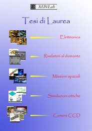
Figure: Brightest sources in the gamma-ray sky are: <strong>compact</strong> binaries, Pulsar Wind Nebulae, blazars.<br />
L. Del Zanna <strong>Relativistic</strong> <strong>Astrophysics</strong> <strong>and</strong> <strong>compact</strong> <strong>objects</strong> 7 / 181
High Energy <strong>Astrophysics</strong><br />
The theory of relativity<br />
Applications to <strong>compact</strong> <strong>objects</strong><br />
The electromagnetic spectrum<br />
Useful physical constants (cgs units):<br />
c = 3.0 10 10 cm s −1<br />
G = 6.7 10 −8 dyne cm 2 g −2<br />
h = 6.6 10 −27 erg s<br />
e = 4.8 10 −10 statcoulomb<br />
me = 9.1 10 −28 g<br />
mp = 1.7 10 −24 g<br />
kB = 1.4 10 −16 erg K −1<br />
σ = 5.7 10 −5 erg s −1 cm −2 K −4<br />
M⊙ = 2.0 10 33 g<br />
R⊙ = 7.0 10 10 cm<br />
L⊙ = 3.8 10 33 erg s −1<br />
1 pc = 3.1 10 18 cm<br />
1 AU = 1.5 10 13 cm<br />
1 yr = 3.2 10 7 s<br />
1 eV = 1.6 10 −12 erg<br />
Figure: The electromagnetic spectrum in <strong>di</strong>fferent<br />
photon energy units. The relations are<br />
E = hν = hc/λ = kB T.<br />
L. Del Zanna <strong>Relativistic</strong> <strong>Astrophysics</strong> <strong>and</strong> <strong>compact</strong> <strong>objects</strong> 8 / 181
High Energy <strong>Astrophysics</strong><br />
The theory of relativity<br />
Applications to <strong>compact</strong> <strong>objects</strong><br />
Supernovae <strong>and</strong> supernova remnants<br />
Supernovae (SNe) are catastrophic explosions of<br />
stars, where the energies involved (Ekin ∼ 10 51 erg)<br />
are about the whole energy ra<strong>di</strong>ated by the<br />
progenitor in its entire life. They are certainly the<br />
high energy events stu<strong>di</strong>ed over the longest time.<br />
Historical (galactic) events were recorded in 1006,<br />
1054, 1181, 1572, 1604, <strong>and</strong> 1680 (1987 in LMC).<br />
Accor<strong>di</strong>ng to SN lightcurves <strong>and</strong> spectra, there are<br />
several types of events. Very important is the class<br />
of type Ia SNe, produced by explosions of white<br />
dwarves in binary systems, where the <strong>di</strong>mming<br />
rate is related to the peak luminosity, thus can be<br />
employed as cosmological st<strong>and</strong>ard c<strong>and</strong>les.<br />
The other classes are characterized by core<br />
collapse: for stars with M > 8 M⊙, once the iron<br />
core has reached the Ch<strong>and</strong>rasekhar mass of<br />
1.44 M⊙, a rapid collapse sets in until a proto<br />
neutron star with ρnuc = 2.6 10 14 g cm −3 <strong>and</strong><br />
T ∼ 10 11 K is formed. Most of the energy is carried<br />
away by neutrinos, then material starts to bounce<br />
back lea<strong>di</strong>ng to the explosion of the outer layers.<br />
Figure: Different lightcurves for type Ia<br />
<strong>and</strong> II SNe <strong>and</strong> the cartoon of<br />
core-collapse for type II SNe.<br />
L. Del Zanna <strong>Relativistic</strong> <strong>Astrophysics</strong> <strong>and</strong> <strong>compact</strong> <strong>objects</strong> 9 / 181
High Energy <strong>Astrophysics</strong><br />
The theory of relativity<br />
Applications to <strong>compact</strong> <strong>objects</strong><br />
A supernova event creates a remnant (SNR) that<br />
may shine for up to 10 5 years, while <strong>di</strong>luting stellar<br />
metal-enriched material in the ISM. The forward<br />
shock of a SNR is also a site for particle<br />
acceleration. In 1934, Baade <strong>and</strong> Zwicky, other<br />
than pre<strong>di</strong>cting the existence of NSs, also<br />
estabilished the supernova para<strong>di</strong>gm: the galactic<br />
cosmic rays (up to 10 15 eV) can be produced using<br />
a small fraction of SN energy.<br />
Galactic cosmic rays have an energy density<br />
uCR ∼ 1 eV cm −3 in a volume Vgal ∼ 200 kpc 3 <strong>and</strong><br />
have a correspon<strong>di</strong>ng escape time of tesc ∼ 10 7 yr.<br />
The rate of production by SNe must be<br />
uCR Vgal/tesc ηESN/tSN,<br />
<strong>and</strong> for ESN ∼ 10 53 erg <strong>and</strong> tSN ∼ 100 yr, an<br />
efficiency of η = 0.05 seems to be enough.<br />
Observations of gamma rays from SNRs due to<br />
hadronic decay would provide the final proof of the<br />
para<strong>di</strong>gm.<br />
Figure: Composite images of the<br />
Tycho <strong>and</strong> Kepler SNRs.<br />
L. Del Zanna <strong>Relativistic</strong> <strong>Astrophysics</strong> <strong>and</strong> <strong>compact</strong> <strong>objects</strong> 10 / 181
High Energy <strong>Astrophysics</strong><br />
The theory of relativity<br />
Applications to <strong>compact</strong> <strong>objects</strong><br />
A special class of SNRs is provided by plerions, or<br />
Pulsar Wind Nebulae (PWNe). Their prototype is the<br />
Crab Nebula (M1, in the Taurus), the SNR of the 1054<br />
supernova observed by the Chinese astronomers.<br />
Other than the usual outer shell, due to the blast wave<br />
interacting with ISM (threaded by optical filaments due<br />
to Rayleigh-Taylor instabilities), the central part is filled<br />
with a hot bubble produced at the termination shock by<br />
the conversion of kinetic energy of the ultrarelativistic<br />
pulsar wind into heat <strong>and</strong> particles. In 2000 the X-ray<br />
Ch<strong>and</strong>ra satellite <strong>di</strong>scovered jets in many PWNe.<br />
PWNe emit non-thermal emission at all wavelengths,<br />
synchrotron ra<strong>di</strong>ation from ra<strong>di</strong>o to gamma<br />
(ultrarelativistic electrons spiralling along magnetic<br />
fields) <strong>and</strong> Inverse Compton (same electrons<br />
interacting with background photons) from GeV to PeV<br />
photon energies. Typical PWN luminosities are<br />
L ∼ 10 38 erg s −1 . Just before the <strong>di</strong>scovery of pulsars,<br />
Franco Pacini pre<strong>di</strong>cted that a young fast rotating<br />
magnetized NS could release via <strong>di</strong>pole ra<strong>di</strong>ation the<br />
right amount of energy to power the Crab Nebula.<br />
Figure: Optical <strong>and</strong> X-ray image<br />
of the Crab Nebula <strong>and</strong> its<br />
multiwavelength spectrum.<br />
L. Del Zanna <strong>Relativistic</strong> <strong>Astrophysics</strong> <strong>and</strong> <strong>compact</strong> <strong>objects</strong> 11 / 181
Pulsars <strong>and</strong> magnetars<br />
High Energy <strong>Astrophysics</strong><br />
The theory of relativity<br />
Applications to <strong>compact</strong> <strong>objects</strong><br />
Pulsars <strong>and</strong> magnetars are the most spectacular<br />
manifestations of NSs, the relic of SN explosions.<br />
Pulsars were <strong>di</strong>scovered in 1967 by Jocelyn Bell, a<br />
PhD student, as sources of extremely perio<strong>di</strong>c<br />
ra<strong>di</strong>o signals. Now we know about 2000 pulsars,<br />
all of them in our Galaxy. If pulsars are collapsed<br />
NSs, we expect a typical ra<strong>di</strong>us<br />
R ∼ (M⊙/ρnuc) 1/3 ∼ 10 km,<br />
<strong>and</strong> from the conservation of angular momentum<br />
<strong>and</strong> magnetic flux<br />
ΩR 2 = const, BR 2 = const,<br />
we derive that a newly born pulsar has P ∼ 1 ms<br />
<strong>and</strong> B ∼ 10 12 G. The perio<strong>di</strong>c signal is due to<br />
some sort of (non-thermal) emission from the<br />
poles of the rotating magnetosphere, making an<br />
angle α with the rotation axis <strong>and</strong> pointing<br />
perio<strong>di</strong>cally towards the Earth.<br />
Figure: Cartoon of a pulsar. The<br />
pulsed ra<strong>di</strong>o emission is produced at<br />
the poles of the magnetosphere.<br />
L. Del Zanna <strong>Relativistic</strong> <strong>Astrophysics</strong> <strong>and</strong> <strong>compact</strong> <strong>objects</strong> 12 / 181
High Energy <strong>Astrophysics</strong><br />
The theory of relativity<br />
Applications to <strong>compact</strong> <strong>objects</strong><br />
Let us now describe the Pacini-Gold model of the<br />
rotating magnetic <strong>di</strong>pole in vacuum. If z is the<br />
rotation axis, the magnetic moment is<br />
m = (BpR 3 /2)(sin α cos ωt, sin α sin ωt, cos α),<br />
<strong>and</strong> the ra<strong>di</strong>ated EM energy in time is<br />
˙E = −(2/3c 3 )| ¨ m| 2 = −B 2 p R6 ω 4 sin 2 α/6c 3 ,<br />
that must be compensated by rotational energy<br />
losses<br />
˙Erot = Iω ˙ω ⇒ ˙ω = −Kω 3 .<br />
Imme<strong>di</strong>ate observable quantities are the period<br />
P = 2π/ω <strong>and</strong> its slowdown rate ˙P. Thanks to this<br />
simple model, a pulsar in the P − ˙P <strong>di</strong>agram has a<br />
ready estimate for the following quantities<br />
˙E ∼ ˙P/P 3 <br />
, Bp sin α ∼ P ˙P, τ ∼ P/ ˙P.<br />
Millisecond pulsars with low magnetic fields are<br />
believed to be recycled old <strong>objects</strong>, spun up by<br />
accretion in a binary system.<br />
Figure: The P − ˙P <strong>di</strong>agram for pulsars.<br />
Only the blue region allows the ra<strong>di</strong>o<br />
emission to operate.<br />
L. Del Zanna <strong>Relativistic</strong> <strong>Astrophysics</strong> <strong>and</strong> <strong>compact</strong> <strong>objects</strong> 13 / 181
High Energy <strong>Astrophysics</strong><br />
The theory of relativity<br />
Applications to <strong>compact</strong> <strong>objects</strong><br />
We know that NSs with a B ∼ 10 12 G magnetic<br />
field are born quite naturally in core-collapse<br />
supernovae. What happens if in the hot proto NS<br />
dynamo sets in <strong>and</strong> B is further amplified? For an<br />
initial period of 1 ms we expect B ∼ 10 15 G, so that<br />
the corona of such magnetar would contain an<br />
energy<br />
Emag ∼ (B 2 /8π)(4π/3)R 3 ∼ 10 48 erg.<br />
Giant flares associated to magnetic field<br />
reconnection events may be observed as<br />
gamma-ray bursts.<br />
We believe that Soft Gamma Repeaters (SGRs,<br />
<strong>and</strong> the lower energy class of Anomalous X-ray<br />
Pulsars, AXPs) may be the proof: sudden releases<br />
of gamma rays of 10 46 erg in a second or less<br />
(more than for SNe!), followed by oscillations<br />
related to the NS rotation. Such high magnetic<br />
fields are confirmed by the measure of rapid<br />
spin-down rates, lea<strong>di</strong>ng to rather long periods<br />
(P ∼ 5 − 8 s).<br />
Figure: A cartoon of a magnetar <strong>and</strong><br />
the lightcurve of a SGR giant flare.<br />
L. Del Zanna <strong>Relativistic</strong> <strong>Astrophysics</strong> <strong>and</strong> <strong>compact</strong> <strong>objects</strong> 14 / 181
Compact binary systems<br />
High Energy <strong>Astrophysics</strong><br />
The theory of relativity<br />
Applications to <strong>compact</strong> <strong>objects</strong><br />
About half of all stars are found in binary (or<br />
multiple) systems, when at least one of the<br />
members is a <strong>compact</strong> object (NS or BH) we call<br />
them <strong>compact</strong> binary systems of X-ray binaries.<br />
When a young, O/B-type, luminous (L > L⊙) <strong>and</strong><br />
massive star (M > 10M⊙) is the donor companion,<br />
a strong stellar wind is present <strong>and</strong> the accretion is<br />
due to the transonic Bon<strong>di</strong>-Hoyle mechanism,<br />
mo<strong>di</strong>fied by relative rotation (HMXB systems).<br />
These systems often show rather regular X-ray<br />
pulsations.<br />
When an evolved, low-mass star that has<br />
exp<strong>and</strong>ed to fill its Roche lobe is the donor star,<br />
accretion occurs via an accretion <strong>di</strong>sk (LMXB<br />
systems). From the emitted ra<strong>di</strong>ation we can infer<br />
the presence of coronal <strong>di</strong>sk winds, transient hot<br />
spots, <strong>and</strong> of quasi-perio<strong>di</strong>c oscillations (QPOs),<br />
related to the dynamics of the <strong>di</strong>sk <strong>and</strong> of the<br />
accretion. These systems are a necessary<br />
evolution step towards millisecond pulsars (spun<br />
up by accretion) <strong>and</strong> binary pulsars.<br />
Figure: Doppler broadened lines due<br />
to winds from an accreting torus <strong>and</strong><br />
high-mass <strong>and</strong> low-mass X-ray binary<br />
systems.<br />
L. Del Zanna <strong>Relativistic</strong> <strong>Astrophysics</strong> <strong>and</strong> <strong>compact</strong> <strong>objects</strong> 15 / 181
High Energy <strong>Astrophysics</strong><br />
The theory of relativity<br />
Applications to <strong>compact</strong> <strong>objects</strong><br />
Binary NS-NS systems (at least one of them must<br />
be a pulsar in order to be detected!) are unique<br />
laboratories for testing General Relativity (GR).<br />
The famous Hulse-Taylor system shows an orbital<br />
decay due to emission of gravitational waves<br />
(GWs), to date only this type of in<strong>di</strong>rect proof is<br />
available. Moreover, post-Newtonian parameters<br />
such as periastron advance, gravitational redshift<br />
<strong>and</strong> time <strong>di</strong>lation, change in orbital period <strong>and</strong><br />
Shapiro delay can be measured <strong>and</strong> used to infer<br />
the single NS masses.<br />
In 2003/4 the first double pulsar system was<br />
<strong>di</strong>scovered, with an orbital period of just 2.4 h! GR<br />
effects are enhanced <strong>and</strong> the relative motions<br />
allow us to even probe the one pulsar’s<br />
magnetosphere: in this fantastic astrophysical<br />
laboratory it has been proved that plasma is<br />
trapped in the closed magnetic field <strong>di</strong>pole within<br />
the light cylinder.<br />
Figure: Emission of GWs in the<br />
Hulse-Taylor binary <strong>and</strong> General<br />
Relativity effects measured in the<br />
double pulsar system.<br />
L. Del Zanna <strong>Relativistic</strong> <strong>Astrophysics</strong> <strong>and</strong> <strong>compact</strong> <strong>objects</strong> 16 / 181
Gamma Ray Bursts<br />
High Energy <strong>Astrophysics</strong><br />
The theory of relativity<br />
Applications to <strong>compact</strong> <strong>objects</strong><br />
Gamma Ray Bursts (GRBs) were <strong>di</strong>scovered in<br />
1967 by the USA Vela satellites, looking for<br />
gamma emission due to nuclear experiments.<br />
However, only in 1973 the <strong>di</strong>scovery was made<br />
public: a cold war gift to Astronomy!<br />
Lightcurves of GRBs are very irregular, duration<br />
varies from 10 −2 to 10 3 seconds. Variability occurs<br />
on τ ∼ 1 ms scales, then the typical size of the<br />
source must be, to preserve coherency of the<br />
signal<br />
R < c τ 300 km,<br />
comparable to NS or stellar mass BH ra<strong>di</strong>i. Until<br />
the 80s there was a general consensus that the<br />
bursters were NSs in our Galaxy.<br />
From the count <strong>di</strong>stribution in duration a clear<br />
<strong>di</strong>stinction between short GRBs (less than 2 s) <strong>and</strong><br />
long GRBs (more than 2 s) can be made. Spectra<br />
are also <strong>di</strong>fferent, those of short GRBs are harder<br />
(larger fraction of high-energy photons).<br />
Figure: Lightcurves from several<br />
GRBs <strong>and</strong> <strong>di</strong>stribution in duration.<br />
L. Del Zanna <strong>Relativistic</strong> <strong>Astrophysics</strong> <strong>and</strong> <strong>compact</strong> <strong>objects</strong> 17 / 181
High Energy <strong>Astrophysics</strong><br />
The theory of relativity<br />
Applications to <strong>compact</strong> <strong>objects</strong><br />
During the 90s we had the proof that GRBs are<br />
actually <strong>di</strong>stant events originated in other galaxies.<br />
BATSE found a perfectly isotropic <strong>di</strong>stribution in<br />
the sky, <strong>and</strong> in 1997 the Italian-Dutch BeppoSAX<br />
mission measured the first X-ray afterglow<br />
associated with a GRB, apparently related to a<br />
faint galaxy. Later also ra<strong>di</strong>o <strong>and</strong> optical afterglows<br />
were found, <strong>and</strong> nowadays Swift currently<br />
measures spectral lines cosmological redshifts<br />
(the record is z = 9.4, observed in 2010). The rate<br />
is one GRB every 10 7 years per galaxy.<br />
Of course this created a problem: some GRBs<br />
have been observed with astonishing isotropized<br />
energies of Eiso = 4.5 10 54 erg, even more than<br />
M⊙c 2 = 1.8 10 54 erg. Only if we assume that the<br />
observed ra<strong>di</strong>ation comes from a jet of half<br />
aperture θjet pointing towards us we can save the<br />
situation, since<br />
Etrue<br />
Eiso<br />
= ∆Ω<br />
4π<br />
= 2 · 2π<br />
4π<br />
θjet<br />
0<br />
sin θdθ θ2<br />
jet<br />
2 ,<br />
lea<strong>di</strong>ng to reduction factors of about 100.<br />
Figure: Proofs of the extragalactic<br />
origin of GRBs: BATSE <strong>and</strong> the first<br />
afterglow by BeppoSAX.<br />
L. Del Zanna <strong>Relativistic</strong> <strong>Astrophysics</strong> <strong>and</strong> <strong>compact</strong> <strong>objects</strong> 18 / 181
High Energy <strong>Astrophysics</strong><br />
The theory of relativity<br />
Applications to <strong>compact</strong> <strong>objects</strong><br />
What is the origin of GRBs? Soon after their <strong>di</strong>scovery it<br />
was pre<strong>di</strong>cted a connection with the death of massive stars<br />
<strong>and</strong> supernova events. The smoking gun was in 2003,<br />
when a supernova occurred 6 days later in the same<br />
position of a bright GRB, confirming a similar event<br />
observed by AGILE in 1998. The most plausible model for<br />
long GRBs is that of a collapsar: a massive iron core<br />
(M > 10M⊙) of a rapidly rotating Wolf-Rayet star may<br />
collapse into a Kerr BH accreting material from a torus.<br />
Polar relativistic jets are believed to be collimated by<br />
magnetic fields <strong>and</strong> later escape the stellar progenitor.<br />
Short GRBs have been observed by Swift from 2004 to be<br />
associated to elliptical galaxies (no young massive stars,<br />
many stellar relics). In a close binary NS-NS system, after<br />
a long inspiral phase, the final merging produces a Kerr BH<br />
surrounded by a T = 10 10 K hot <strong>di</strong>sk, <strong>and</strong> jets are<br />
expected to form as in the previous case.<br />
In both cases, the available gravitational bin<strong>di</strong>ng energy<br />
seems to be more than enough:<br />
E GM2<br />
R<br />
3 1053<br />
M<br />
M⊙<br />
2 −1 R<br />
erg.<br />
10 km<br />
Figure: Mainstream models for<br />
GRBs: collapsar for long GRBs<br />
<strong>and</strong> binary NS-NS merger for<br />
short GRBs.<br />
L. Del Zanna <strong>Relativistic</strong> <strong>Astrophysics</strong> <strong>and</strong> <strong>compact</strong> <strong>objects</strong> 19 / 181
High Energy <strong>Astrophysics</strong><br />
The theory of relativity<br />
Applications to <strong>compact</strong> <strong>objects</strong><br />
We have seen that Γ > 100 relativistic jets must<br />
form in small polar angles θjet < 10 ◦ . We shall see<br />
that ra<strong>di</strong>ation from a moving source is beamed<br />
within an angle θ ∼ 1/Γ, this leads to observable<br />
change of slopes in lightcurves as the jet slows<br />
down (achromatic breaks).<br />
The model for a sudden release of relativistic<br />
energy with<br />
η = E/Mc 2 = e/ρc 2 ≫ 1,<br />
<strong>and</strong> of its propagation is said fireball. The GRB<br />
gamma prompt emission is assumed to be<br />
non-thermal ra<strong>di</strong>ation produced in colli<strong>di</strong>ng shock<br />
fronts within the jet. The X-ray <strong>and</strong> optical<br />
afterglow occurs after interaction with ISM.<br />
Viewing angle effects may also explain lower<br />
energy events (X-Ray Rich GRBs <strong>and</strong> X-Ray<br />
Flashes), since relativistic beaming <strong>and</strong> Doppler<br />
effects (enhancing E <strong>and</strong> ν, respectively) are<br />
reduced for jets observed off-axis. We shall<br />
<strong>di</strong>scuss these effects later in the course.<br />
Figure: The fireball model <strong>and</strong><br />
relativistic effects for lower energy<br />
events.<br />
L. Del Zanna <strong>Relativistic</strong> <strong>Astrophysics</strong> <strong>and</strong> <strong>compact</strong> <strong>objects</strong> 20 / 181
Active Galactic Nuclei<br />
High Energy <strong>Astrophysics</strong><br />
The theory of relativity<br />
Applications to <strong>compact</strong> <strong>objects</strong><br />
Active Galactic Nuclei (AGNs) are the central part<br />
(less than 10 ly) of active galaxies, about 3% of the<br />
known galaxies. They were <strong>di</strong>scovered <strong>and</strong><br />
recognized as extragalactic sources between the<br />
50s <strong>and</strong> 60s. Huge zoology: ra<strong>di</strong>o galaxies,<br />
quasars (QSOs), Seyfert, BL Lac, Markarian,<br />
blazars...<br />
The main characteristics (not necessarily all<br />
present in all classes) of active galaxies hosting<br />
AGNs are:<br />
<strong>compact</strong> size, luminous center,<br />
spectra with strong emission lines,<br />
strong Doppler-broadened emission lines,<br />
strong ultraviolet emission from center,<br />
strong non-thermal emission,<br />
jets <strong>and</strong> double ra<strong>di</strong>o lobes,<br />
short timescale variability at all wavelengths.<br />
Figure: Composite image of<br />
Centaurus A.<br />
L. Del Zanna <strong>Relativistic</strong> <strong>Astrophysics</strong> <strong>and</strong> <strong>compact</strong> <strong>objects</strong> 21 / 181
High Energy <strong>Astrophysics</strong><br />
The theory of relativity<br />
Applications to <strong>compact</strong> <strong>objects</strong><br />
Typical bolometric luminosities for quasars are<br />
L ∼ 10 46 erg s −1 ,<br />
at least 100 times st<strong>and</strong>ard galaxies,<br />
concentrated in a very <strong>compact</strong> region. Time<br />
variability is observed in some AGNs to be as<br />
small as τ ∼ 1h, thus the source size must be,<br />
to preserve coherence of the signal<br />
R < cτ 3.5 10 −5 pc,<br />
which is about the size of our Solar System!<br />
Figure: VLBA observations of<br />
Keplerian motions in an AGN <strong>di</strong>sk.<br />
Accretion from a <strong>di</strong>sk onto a supermassive black hole (SMBH) is the answer. Consider<br />
matter ∆M = ˙M∆t falling ra<strong>di</strong>ally from infinity <strong>and</strong> converting its kinetic energy into heat<br />
<strong>and</strong> ra<strong>di</strong>ation when it stops at a ra<strong>di</strong>us R. The available power is<br />
L = 1 ˙Mv 2<br />
2 ff = GM ˙M/R = ξ ˙Mc 2 ,<br />
where ξ is the efficiency. For a SMBH with M ∼ 10 8 M⊙ the Schwarzschild ra<strong>di</strong>us is<br />
Rs = 2GM/c 2 10 −5 pc,<br />
<strong>and</strong> ξ = 1/2. For comparison, nuclear fusion (<strong>di</strong>rect conversion of rest mass to energy) in<br />
the Sun leads to ξ = 0.007. The observed luminosity can be reached with ˙M ∼ 1 M⊙ yr −1 .<br />
L. Del Zanna <strong>Relativistic</strong> <strong>Astrophysics</strong> <strong>and</strong> <strong>compact</strong> <strong>objects</strong> 22 / 181
High Energy <strong>Astrophysics</strong><br />
The theory of relativity<br />
Applications to <strong>compact</strong> <strong>objects</strong><br />
Another clear in<strong>di</strong>cation that accretion onto a<br />
supermassive central object is what powers AGNs<br />
comes from the observation that AGN luminosities are<br />
always smaller than the so-called Ed<strong>di</strong>ngton limit<br />
LEdd = 4πGMmpc<br />
10<br />
σT<br />
46<br />
<br />
M<br />
108 <br />
erg s<br />
M⊙<br />
−1 ,<br />
where σT = 6.65 10 −25 cm 2 is the Thomson cross<br />
section for electrons <strong>and</strong> where the mass of the SMBH<br />
is inferred either from the bulge luminosity or from its<br />
virial velocity <strong>di</strong>spersion.<br />
The Ed<strong>di</strong>ngton limit is due to the back reaction of the<br />
ra<strong>di</strong>ation produced by the extremely hot accreting gas.<br />
In a fully ionized plasma, protons <strong>and</strong> electrons are<br />
bound to move together, then the limit is found by<br />
equating the gravitational <strong>and</strong> ra<strong>di</strong>ation forces<br />
F = GMmp<br />
r 2<br />
L/c<br />
= σT ,<br />
4πr2 where gravity on electrons <strong>and</strong> ra<strong>di</strong>ation pressure on<br />
protons (σ ∝ m −2 ) have been neglected.<br />
Figure: Hubble image of a torus<br />
in a galactic center; <strong>di</strong>stribution of<br />
AGNs in the L − MBH plane.<br />
L. Del Zanna <strong>Relativistic</strong> <strong>Astrophysics</strong> <strong>and</strong> <strong>compact</strong> <strong>objects</strong> 23 / 181
High Energy <strong>Astrophysics</strong><br />
The theory of relativity<br />
Applications to <strong>compact</strong> <strong>objects</strong><br />
We have seen that a SMBH accreting mass from a<br />
torus is a good c<strong>and</strong>idate to explain AGN<br />
energetics. Other observational features like<br />
emission lines <strong>and</strong> can be explained within a<br />
unified model by changing some parameters (most<br />
notably the viewing angle).<br />
One important open question is, how are the polar<br />
jets accelerated to ultrarelativistic speeds? Two of<br />
the most successful mechanisms involve the<br />
presence of the magnetic field:<br />
Magnetocentrifugal due to <strong>di</strong>sk’s field,<br />
Bl<strong>and</strong>ford-Znajek due to extraction of energy<br />
from the rotating BH’s ergosphere.<br />
Jets must be relativistic because we observe<br />
apparent superluminal velocities in the plane of the<br />
sky from blobs in jets with Vjet c almost pointing<br />
towards us (blazars). We are going to see that<br />
vapp ≤ Γjetc, ⇒ Γjet ≥ vapp/c,<br />
<strong>and</strong>, for instance, in 3C 373 we find<br />
vapp 10c ⇒ Γjet ≥ 10 ⇒ Vjet/c = (1−1/Γ 2<br />
jet )1/2 ≥ 99%!<br />
Figure: The jet of M87 with features in<br />
apparent superluminal motion.<br />
L. Del Zanna <strong>Relativistic</strong> <strong>Astrophysics</strong> <strong>and</strong> <strong>compact</strong> <strong>objects</strong> 24 / 181
High Energy <strong>Astrophysics</strong><br />
The theory of relativity<br />
Applications to <strong>compact</strong> <strong>objects</strong><br />
The demonstration does not involve relativity, but<br />
only geometry under the assumption of a finite<br />
light propagation speed. The apparent velocity in<br />
the plane of the sky is<br />
vapp =<br />
Vτ sin θ<br />
τ − Vτ cos θ/c =<br />
V sin θ<br />
1 − (V/c) cos θ ,<br />
where the first denominator is the arrival time of<br />
photons emitted in an interval τ. For a given speed<br />
V of the jet, vapp is a function of the observing<br />
angle θ. This function has a maximum for<br />
where<br />
cos θc = V/c, sin θc = Γ −1 ,<br />
vapp(θc) =<br />
V/Γ<br />
= ΓV,<br />
1 − (V/c) 2<br />
thus for V c the maximum observed speed is<br />
basically vapp ≤ Γc, as used in the previous slide.<br />
Thus, special relativity is not violated. On the<br />
contrary, we have a clear demonstration of the<br />
presence of relativistic velocities.<br />
Figure: Explanation of superluminal<br />
motions of relativistic jets. Below: the<br />
function vapp(θ)/c for <strong>di</strong>fferent values<br />
of V (or Γ).<br />
L. Del Zanna <strong>Relativistic</strong> <strong>Astrophysics</strong> <strong>and</strong> <strong>compact</strong> <strong>objects</strong> 25 / 181
High Energy <strong>Astrophysics</strong><br />
The theory of relativity<br />
Applications to <strong>compact</strong> <strong>objects</strong><br />
Special Relativity<br />
General Relativity: the Principle of Equivalence<br />
Physics in an external gravitational field<br />
The Einstein field equations<br />
Part II: the theory of relativity<br />
L. Del Zanna <strong>Relativistic</strong> <strong>Astrophysics</strong> <strong>and</strong> <strong>compact</strong> <strong>objects</strong> 26 / 181
High Energy <strong>Astrophysics</strong><br />
The theory of relativity<br />
Applications to <strong>compact</strong> <strong>objects</strong><br />
Special Relativity<br />
General Relativity: the Principle of Equivalence<br />
Physics in an external gravitational field<br />
The Einstein field equations<br />
Special Relativity<br />
L. Del Zanna <strong>Relativistic</strong> <strong>Astrophysics</strong> <strong>and</strong> <strong>compact</strong> <strong>objects</strong> 27 / 181
High Energy <strong>Astrophysics</strong><br />
The theory of relativity<br />
Applications to <strong>compact</strong> <strong>objects</strong><br />
Special Relativity: introduction<br />
Special Relativity<br />
General Relativity: the Principle of Equivalence<br />
Physics in an external gravitational field<br />
The Einstein field equations<br />
The laws of Newtonian mechanics are invariant in any inertial system (where a body not<br />
subject to forces moves with uniform velocity), this is known as the Galilean principle of<br />
relativity. Given a transformation from an inertial system (t, x) to another one (t ′ , x ′ )<br />
moving at constant speed v<br />
t ′ = t, x ′ = x − vt, (1.1)<br />
velocities <strong>and</strong> accelerations transform as u ′ = u − v ⇒ a ′ = a, so there is no way to detect<br />
a <strong>di</strong>fference in any force obeying F = ma.<br />
This is not true for Maxwell’s equations, containing the speed of light c. For example, the<br />
equation for electromagnetic waves<br />
[−(1/c 2 )∂ 2 t + ∇2 ]f(t, x) = 0, (1.2)<br />
is not invariant, since substituting ∇ = ∇ ′ , ∂t = ∂t ′ − v · ∇′ we get something quite <strong>di</strong>fferent.<br />
Thus, at the end of the 19 th century people were convinced that the light propagates in a<br />
privileged system (that of ether). In 1887 Michelson <strong>and</strong> Morley demonstrated that, within<br />
5 km s −1 , the velocity of light <strong>di</strong>d not change during Earth’s orbital motion. However, in 1892<br />
Lorentz proposed that bo<strong>di</strong>es contract like l = l0(1 − v 2 /c 2 ) 1/2 in the <strong>di</strong>rection of motion<br />
respect to ether, explaining the negative result, <strong>and</strong> later, with Poincaré, proposed the<br />
famous Lorentz transformations for <strong>di</strong>stribution of moving charges, that leave Maxwell’s<br />
equations invariant <strong>and</strong> pre<strong>di</strong>ct the contraction. The <strong>di</strong>scovery of the electron seemed to<br />
support these ad hoc hypotheses for a while, until experiments of light refraction in moving<br />
liquids led to a complete rejection of the ether option.<br />
L. Del Zanna <strong>Relativistic</strong> <strong>Astrophysics</strong> <strong>and</strong> <strong>compact</strong> <strong>objects</strong> 28 / 181
High Energy <strong>Astrophysics</strong><br />
The theory of relativity<br />
Applications to <strong>compact</strong> <strong>objects</strong><br />
Special Relativity<br />
General Relativity: the Principle of Equivalence<br />
Physics in an external gravitational field<br />
The Einstein field equations<br />
The Principle of Relativity <strong>and</strong> Lorentz transformations<br />
In 1905 Albert Einstein (1879 - 1955) proposed a ra<strong>di</strong>cal solution: by exten<strong>di</strong>ng Galilean<br />
relativity <strong>and</strong> assuming the vali<strong>di</strong>ty of Maxwell’s equations, he mo<strong>di</strong>fied Newton’s laws <strong>and</strong><br />
the concepts of absolute time <strong>and</strong> space. The postulates of Special Relativity are:<br />
1 Principle of Relativity. The laws of nature are the same in any inertial system.<br />
2 The speed of light is also the same in any inertial system, independently of the relative<br />
motion between the source <strong>and</strong> the observer.<br />
Here special means that we are assuming the existence of global inertial frames, where<br />
bo<strong>di</strong>es not subject to forces maintain their status of motion with uniform velocity. In General<br />
Relativity this will be true just locally. From now on c = 1 <strong>and</strong> t → ct will be a <strong>di</strong>stance.<br />
Galilean transformations are replaced by Lorentz transformations<br />
where<br />
t ′ = γ(t − v · x), x ′ = γ(x − vt), x ′ ⊥ = x⊥, (1.3)<br />
γ := (1 − v 2 ) −1/2 , (1.4)<br />
is the Lorentz factor. Notice that time <strong>and</strong> space are now mixed up (in the <strong>di</strong>rection parallel<br />
to v), this is the only way to have a constant speed of light <strong>and</strong> invariance of Maxwell’s<br />
equations. The inverse relations are found by swapping (t, x) with (t ′ , x ′ ) <strong>and</strong> the sign of v.<br />
These transformations can be further generalized to translations in time <strong>and</strong> to rotations<br />
(the Poincaré group).<br />
L. Del Zanna <strong>Relativistic</strong> <strong>Astrophysics</strong> <strong>and</strong> <strong>compact</strong> <strong>objects</strong> 29 / 181
High Energy <strong>Astrophysics</strong><br />
The theory of relativity<br />
Applications to <strong>compact</strong> <strong>objects</strong><br />
Special Relativity<br />
General Relativity: the Principle of Equivalence<br />
Physics in an external gravitational field<br />
The Einstein field equations<br />
Basic kinematic consequences of Lorentz transformations<br />
The imme<strong>di</strong>ate consequences of Lorentz transformations are ra<strong>di</strong>cal changes in the<br />
concepts of simultaneity of events, measures of lengths <strong>and</strong> time intervals.<br />
Loss of simultaneity. Consider light emitted isotropically from a point B along x ′ ,<br />
reaching points A <strong>and</strong> C along the same axis with x ′ A < x′ B < x′ C <strong>and</strong><br />
x ′ C − x′ B = x′ B − x′ A = ∆l0, where for simplicity we assume v x x ′ . For the observer<br />
in B in the primed system the photons will reach A <strong>and</strong> C simultaneously, since the<br />
speed of light is unchanged by the motion. For an observer still in B at the moment of<br />
emission but steady in the unprimed system the photons will reach A first, thus the<br />
concept of simultaneity is relative.<br />
Contraction of length. In the same example, the <strong>di</strong>stance observed in the steady frame<br />
is, accor<strong>di</strong>ng to (1.3),<br />
xB − xA = v(tB − tA ) + γ −1 (x ′ B − x′ A ), tA = tB ⇒ ∆l = γ −1 ∆l0 ≤ ∆l0 , (1.5)<br />
where he index 0 in<strong>di</strong>cates the proper length in the rest frame.<br />
Time <strong>di</strong>lation. Similarly, consider an event occurring at the same place in the primed<br />
system, for instance the creation (1) <strong>and</strong> decay (2) of a particle. We find<br />
t2 − t1 = γ[t ′ 2 − t′ 1 + v(x′ 2 − x′ 1 )], x′ 2 = x′ 1 ⇒ ∆t = γ∆t0 ≥ ∆t0 , (1.6)<br />
where the index 0 in<strong>di</strong>cates the proper time in the rest frame. Particles moving at high<br />
Lorentz factors are actually seen to live much longer than steady particles.<br />
L. Del Zanna <strong>Relativistic</strong> <strong>Astrophysics</strong> <strong>and</strong> <strong>compact</strong> <strong>objects</strong> 30 / 181
High Energy <strong>Astrophysics</strong><br />
The theory of relativity<br />
Applications to <strong>compact</strong> <strong>objects</strong><br />
Transformation of velocities <strong>and</strong> aberration<br />
Special Relativity<br />
General Relativity: the Principle of Equivalence<br />
Physics in an external gravitational field<br />
The Einstein field equations<br />
Consider a point with velocity u ′ := dx ′ /dt ′ in the moving frame <strong>and</strong> u := dx/dt in the<br />
observer frame. From the <strong>di</strong>fferentials of the inverse of the relations (1.3) we find<br />
dt = γ(dt ′ + vdx ′ ), dx = γ(dx ′ + vdt ′ ), dy = dy ′ , dz = dz ′ , (1.7)<br />
hence the velocity measured in the laboratory frame is<br />
u =<br />
u ′ + v<br />
1 + v · u ′ , u⊥<br />
u<br />
=<br />
′ ⊥<br />
γ(1 + v · u ′ )<br />
For parallel velocities u1 (= v) <strong>and</strong> u2 (= u ′ ) the composition rule is<br />
. (1.8)<br />
u = u1 + u2<br />
, (1.9)<br />
1 + u1u2<br />
<strong>and</strong> from (1 − u1)(1 − u2) > 0 it is easy to see that u < 1, as expected.<br />
When instead u ′ makes an angle θ ′ 0 with v, we find the formula for relativistic aberration<br />
tan θ = |u⊥|<br />
|u| =<br />
u ′ sin θ ′<br />
γ(u ′ cos θ ′ + v)<br />
, (1.10)<br />
where u ′ = |u ′ |, <strong>and</strong> the azimuthal angle φ remains unchanged. If light is emitted in the<br />
moving system, we have u ′ = 1 in the above formula.<br />
L. Del Zanna <strong>Relativistic</strong> <strong>Astrophysics</strong> <strong>and</strong> <strong>compact</strong> <strong>objects</strong> 31 / 181
High Energy <strong>Astrophysics</strong><br />
The theory of relativity<br />
Applications to <strong>compact</strong> <strong>objects</strong><br />
<strong>Relativistic</strong> beaming <strong>and</strong> relativistic Doppler effect<br />
Special Relativity<br />
General Relativity: the Principle of Equivalence<br />
Physics in an external gravitational field<br />
The Einstein field equations<br />
Consider then a photon with θ ′ = π/2, in the laboratory frame we observe<br />
tan θ = 1/(γv) ⇒ sin θ = 1/γ , (1.11)<br />
<strong>and</strong> for γ ≫ 1 we have θ ∼ 1/γ ≪ 1. Thus, light emitted isotropically in the comoving frame<br />
is observed to be almost entirely collimated along v. This is known as relativistic beaming<br />
<strong>and</strong> it can make a source much brighter compared to isotropic emission.<br />
Consider now light emitted from a source moving at speed v, covering a <strong>di</strong>stance s = vτ<br />
making an angle θ with the line of sight, in the laboratory frame. The classical Doppler<br />
effects (for a limited speed of light!) pre<strong>di</strong>cts a <strong>di</strong>fference in arrival times<br />
∆tA = τ − s cos θ = τ(1 − v cos θ).<br />
If τ = γ/ν0 corresponds to a period of the emitted ra<strong>di</strong>ation, inclu<strong>di</strong>ng relativistic time<br />
<strong>di</strong>lation, the observed frequency will be ν = ∆t−1, that is<br />
A<br />
ν = Dν0, D := [γ(1 − v cos θ)] −1 , (1.12)<br />
where D is called Doppler boosting factor, <strong>and</strong> we may have D ≫ 1.<br />
L. Del Zanna <strong>Relativistic</strong> <strong>Astrophysics</strong> <strong>and</strong> <strong>compact</strong> <strong>objects</strong> 32 / 181
Spacetime intervals<br />
High Energy <strong>Astrophysics</strong><br />
The theory of relativity<br />
Applications to <strong>compact</strong> <strong>objects</strong><br />
Special Relativity<br />
General Relativity: the Principle of Equivalence<br />
Physics in an external gravitational field<br />
The Einstein field equations<br />
In 1908 Minkowski put SR in geometrical terms. The second postulate is the same of<br />
saying that the interval between two spacetime events<br />
∆s 2 := −∆t 2 + ∆x 2 , (1.13)<br />
is invariant under Lorentz transformations. Spacelike separations with ∆s 2 > 0 would<br />
require faster than light signals <strong>and</strong> are causally <strong>di</strong>sconnected, null separations with<br />
∆s 2 = 0 characterize light propagation (<strong>and</strong> it is the equation for the separation surface in<br />
the figure, known as light cone), timelike separations with ∆s 2 < 0 are either in the causal<br />
past or future.<br />
In this latter case it is always possible to define an inertial frame where the two events occur<br />
at the same place (rest frame) <strong>and</strong> the quantity<br />
<br />
∆τ := −∆s2 = γ −1 ∆t (1.14)<br />
is called proper time.<br />
L. Del Zanna <strong>Relativistic</strong> <strong>Astrophysics</strong> <strong>and</strong> <strong>compact</strong> <strong>objects</strong> 33 / 181
High Energy <strong>Astrophysics</strong><br />
The theory of relativity<br />
Applications to <strong>compact</strong> <strong>objects</strong><br />
The Minkowski spacetime <strong>and</strong> the Lorentz group<br />
Special Relativity<br />
General Relativity: the Principle of Equivalence<br />
Physics in an external gravitational field<br />
The Einstein field equations<br />
In general, any (linear) Lorentz transformation between inertial systems x µ := (t, x) <strong>and</strong><br />
x µ′<br />
:= (t ′ , x ′ ), can be written by using the 4 × 4 Jacobian as<br />
x µ′<br />
= Λ µ′<br />
µ x µ , (1.15)<br />
where from now on Greek in<strong>di</strong>ces will in<strong>di</strong>cate spacetime 4-vectors 0123, with x0 ≡ t, <strong>and</strong><br />
we shall make use of Einstein’s summation convention on repeated in<strong>di</strong>ces. In the case of a<br />
simple translation of the primed system along x, the Jacobian is<br />
Λ µ′<br />
µ =<br />
⎛<br />
⎜⎝<br />
γ −γv 0 0<br />
−γv γ 0 0<br />
0 0 1 0<br />
0 0 0 1<br />
The interval definition may be rewritten in <strong>di</strong>fferential form as<br />
⎞<br />
. (1.16)<br />
⎟⎠<br />
ds 2 := ηµνdx µ dx ν , (1.17)<br />
where we define the Minkowski metric tensor as the <strong>di</strong>agonal 4 × 4 array<br />
ηµν := <strong>di</strong>ag{−1, +1, +1, +1} . (1.18)<br />
Note that we shall adopt throughout the signature (−1, +1, +1, +1).<br />
L. Del Zanna <strong>Relativistic</strong> <strong>Astrophysics</strong> <strong>and</strong> <strong>compact</strong> <strong>objects</strong> 34 / 181
High Energy <strong>Astrophysics</strong><br />
The theory of relativity<br />
Applications to <strong>compact</strong> <strong>objects</strong><br />
Special Relativity<br />
General Relativity: the Principle of Equivalence<br />
Physics in an external gravitational field<br />
The Einstein field equations<br />
The 4D space generated by this metric is called Minkowski spacetime M4. The Minkowski<br />
tensor is isotropic, that is invariant in any inertial frame of M4, then det(η) = −1 <strong>and</strong><br />
η −1 ≡ η. Lorentz transformations leave ds ′2 unchanged if <strong>and</strong> only if<br />
Λ µ′<br />
µ Λ ν′<br />
ν ηµ ′ ν ′ = ηµν, (1.19)<br />
where ηµ ′ ν ′ is the same Minkowski tensor defined above, as can be easily checked<br />
ds ′2 = ηµ ′ ν ′ dxµ′ dx ν′<br />
= ηµ ′ ν ′Λµ′ µ dx µ Λ ν′<br />
ν dxν = ηµνdx µ dx ν = ds 2 .<br />
It is instructive to verify that Lorentz transformations in (1.16) satisfy (1.19).<br />
Let us now demonstrate that Lorentz transformations form a group in M4 with respect to<br />
matrix multiplication. In matrix form, the con<strong>di</strong>tion (1.19) becomes<br />
Λ T ηΛ = η . (1.20)<br />
Since det(Λ) 2 = 1, there is always the inverse transformation Λ −1 , given by<br />
This is still a Lorentz transformation, as it satisfies<br />
Λ −1 = ηΛ T η. (1.21)<br />
(Λ −1 ) T ηΛ −1 = (ηΛη)η(ηΛ T η) = η(ΛηΛ T )η = η.<br />
Moreover, if Λ1 <strong>and</strong> Λ2 are Lorentz transformations, then also Λ = Λ2Λ1<br />
Λ T ηΛ = (Λ2Λ1) T η(Λ2Λ1) = Λ T<br />
1 (ΛT<br />
2 ηΛ2)Λ1 = Λ T<br />
1 ηΛ1 = η,<br />
hence these two properties ensure that we have a group.<br />
L. Del Zanna <strong>Relativistic</strong> <strong>Astrophysics</strong> <strong>and</strong> <strong>compact</strong> <strong>objects</strong> 35 / 181
Basics of tensor calculus<br />
High Energy <strong>Astrophysics</strong><br />
The theory of relativity<br />
Applications to <strong>compact</strong> <strong>objects</strong><br />
Special Relativity<br />
General Relativity: the Principle of Equivalence<br />
Physics in an external gravitational field<br />
The Einstein field equations<br />
We now make a mathematical <strong>di</strong>gression, needed to write invariant equations accor<strong>di</strong>ng to<br />
the Principle of Relativity. Given a vector A(x 1 , x 2 ) defined on a surface, not necessarily a<br />
plane, <strong>and</strong> the coor<strong>di</strong>nate basis (e1, e2), this can be decomposed in two ways<br />
A = A 1 e1 + A 2 e2; A1 = A · e1, A2 = A · e2 (A = A1e 1 + A2e 2 ),<br />
where upper (lower) in<strong>di</strong>ces characterize contravariant (covariant) components.<br />
It is possible to switch from one representation to another through the metric tensor <strong>and</strong> its<br />
inverse, defined as (in any number of <strong>di</strong>mensions)<br />
gµν := eµ · eν, g µν gνρ = δ µ ρ, (g µν := e µ · e ν , eµ · e ν = δ ν µ) (1.22)<br />
where δ µ ν is the Kronecker symbol. Imme<strong>di</strong>ate consequences for any vector A = A µ eµ are<br />
Aµ = gµνA ν ; A µ = g µν Aν; A · B = gµνA µ B ν = g µν AµBν = AµB µ . (1.23)<br />
L. Del Zanna <strong>Relativistic</strong> <strong>Astrophysics</strong> <strong>and</strong> <strong>compact</strong> <strong>objects</strong> 36 / 181
High Energy <strong>Astrophysics</strong><br />
The theory of relativity<br />
Applications to <strong>compact</strong> <strong>objects</strong><br />
Special Relativity<br />
General Relativity: the Principle of Equivalence<br />
Physics in an external gravitational field<br />
The Einstein field equations<br />
Consider now a change of coor<strong>di</strong>nate basis, that we write in the form<br />
eµ = eµ ′ Mµ′ µ , (1.24)<br />
where M is the (linear) transformation matrix. Any vector A is an object existing<br />
independently on the particular basis chosen, hence<br />
A = A µ eµ = A µ′ eµ ′ = A µ eµ ′ Mµ′ µ ⇒ A µ′<br />
= M µ′<br />
µ A µ , (1.25)<br />
which is the rule of transformation for contravariant components. Consider now the scalar<br />
product of any two vectors A <strong>and</strong> B, which in turn must be invariant, we have<br />
A · B = A µ Bµ = A µ′<br />
Bµ ′ = Mµ′ µ A µ µ<br />
Bµ ′ ⇒ Bµ ′ = M<br />
µ ′ Bµ, (1.26)<br />
that is covariant vector components transform with (M −1 ) T .<br />
In the Minkowski spacetime M4 we have M µ′<br />
µ = Λ µ′<br />
µ <strong>and</strong> gµν = ηµν. A 4-vector of M4 is any<br />
object V µ that under a Lorentz transformation changes accor<strong>di</strong>ng to V µ′ = Λ µ′<br />
µ V µ , precisely<br />
as the coor<strong>di</strong>nates in (1.15). Note that the simple form of (1.18) provides the properties<br />
V µ = (V 0 , V), Vµ = (V0, V) ⇒ V0 = −V 0 . (1.27)<br />
AµB µ = ηµνA µ B ν = −A 0 B 0 + A · B, (1.28)<br />
where from now on the vector symbols will in<strong>di</strong>cate spatial 3-vectors alone.<br />
L. Del Zanna <strong>Relativistic</strong> <strong>Astrophysics</strong> <strong>and</strong> <strong>compact</strong> <strong>objects</strong> 37 / 181
High Energy <strong>Astrophysics</strong><br />
The theory of relativity<br />
Applications to <strong>compact</strong> <strong>objects</strong><br />
Special Relativity<br />
General Relativity: the Principle of Equivalence<br />
Physics in an external gravitational field<br />
The Einstein field equations<br />
Let us now provide more general definitions, valid in any <strong>di</strong>fferentiable manifold (<strong>and</strong> thus in<br />
GR as well). Let x → x ′ be a general coor<strong>di</strong>nate transformation with non-singular Jacobian<br />
Λ µ′<br />
µ := ∂xµ′<br />
µ′<br />
≡ ∂µx<br />
µ<br />
∂x<br />
, (1.29)<br />
which only for the linear Lorentz transformation coincides with (1.15), with inverse matrix<br />
Λ µ<br />
µ ′ := ∂xµ<br />
∂x µ′ ≡ ∂µ ′ x µ , Λ µ<br />
µ ′ Λ µ′<br />
ν = δ µ ν . (1.30)<br />
A contravariant vector has components V µ transforming as the <strong>di</strong>fferential <strong>di</strong>splacement<br />
dx µ′<br />
= Λ µ′<br />
µ dx µ ⇒ V µ′<br />
= Λ µ′<br />
µ V µ , (1.31)<br />
whereas a covariant vector Vµ transforms as the components of a gra<strong>di</strong>ent of a function<br />
µ<br />
∂µ ′φ = Λ µ ′ µ<br />
∂µφ ⇒ Vµ ′ = Λ µ ′ Vµ. (1.32)<br />
For any mixed tensor, say T µν<br />
λ , we have transformation rules such as<br />
T µ′ ν ′<br />
λ ′ = Λ µ′<br />
µ Λ ν′<br />
ν Λ λ<br />
λ<br />
µν<br />
′ T λ .<br />
Analogies with the previous case are apparent if we let eµ ≡ µ<br />
∂µ, for which eµ ′ = Λ µ ′eµ.<br />
In particular gµν is a fully covariant tensor, while the Kronecker symbol δ µ ν is a mixed tensor<br />
(both of rank 2).<br />
L. Del Zanna <strong>Relativistic</strong> <strong>Astrophysics</strong> <strong>and</strong> <strong>compact</strong> <strong>objects</strong> 38 / 181
High Energy <strong>Astrophysics</strong><br />
The theory of relativity<br />
Applications to <strong>compact</strong> <strong>objects</strong><br />
Special Relativity<br />
General Relativity: the Principle of Equivalence<br />
Physics in an external gravitational field<br />
The Einstein field equations<br />
The next step towards writing invariant equations is how to combine <strong>di</strong>fferent tensors. This<br />
is accomplished through a few simple algebraic operations, here we just provide one<br />
example for each <strong>and</strong> we leave the demonstration of their invariance to the reader.<br />
1 Linear combinations:<br />
2 Direct products:<br />
3 Contractions:<br />
T µ ν := aA µ ν + bB µ ν. (1.33)<br />
µ λ<br />
T ν := A µ νB λ . (1.34)<br />
T µν µ λν<br />
:= T λ . (1.35)<br />
The operation of lowering or raising the in<strong>di</strong>ces falls in these categories, since it involves<br />
contraction of in<strong>di</strong>ces with the metric tensor gµν or its inverse g µν .<br />
An important consequence of these rules is, for example, that the line element<br />
is effectively an invariant (a scalar):<br />
ds 2 := gµνdx µ dx ν , (1.36)<br />
ds ′2 = gµ ′ ν ′ dxµ′ dx ν′<br />
= Λ µ<br />
µ ′Λ ν µ′<br />
ν ′ gµνdx dx ν′<br />
= gµνdx µ dx ν = ds 2 ,<br />
as already found in Minkowskian spacetime where gµν = ηµν, <strong>and</strong> equivalently the scalar<br />
= AµB µ .<br />
product of any two vectors Aµ ′ Bµ′<br />
L. Del Zanna <strong>Relativistic</strong> <strong>Astrophysics</strong> <strong>and</strong> <strong>compact</strong> <strong>objects</strong> 39 / 181
High Energy <strong>Astrophysics</strong><br />
The theory of relativity<br />
Applications to <strong>compact</strong> <strong>objects</strong><br />
Special Relativity<br />
General Relativity: the Principle of Equivalence<br />
Physics in an external gravitational field<br />
The Einstein field equations<br />
Not all quantities appearing in relativity are scalars, vectors, or tensors. An important class<br />
is that of tensor densities. The first example, a scalar density, is the determinant of the<br />
metric tensor (negative for Lorentzian spacetimes, in particular −1 for gµν = ηµν)<br />
g := det(gµν), (1.37)<br />
for which in the transormation rule appears the determinant of the Jacobian<br />
g ′ = Λ −2 g, Λ := det(Λ µ′<br />
µ ) ≡ [det(Λ µ<br />
µ ′ )] −1 ≡ (Λ ′ ) −1 .<br />
A tensor density is similar. In particular, a tensor density of weight w transforms as a tensor<br />
but with an extra factor Λ w . Now, since Λ w = |g| w/2 /|g ′ | w/2 , any tensor density of weight w<br />
multiplied by |g| w/2 is a tensor. One famous example is the volume element dx 4 , for which<br />
d 4 x ′ = Λd 4 x ⇒ |g ′ | 1/2 d 4 x ′ = |g| 1/2 d 4 x, (1.38)<br />
so that |g| 1/2 d 4 x is an invariant volume element. Another case is the Levi-Civita tensor<br />
density ɛµνρσ, which has weight w = −1. Moreover, we may demostrate that<br />
ɛµνρσ = gɛ µνρσ , so that we retrieve tensors by defining<br />
|g| −1/2 ɛµνρσ = −|g| 1/2 ɛ µνρσ = [µνρσ], (1.39)<br />
where [µνρσ] is the completely antisymmetric symbol, which is +1 for any even<br />
permutation of [0123], −1 for any odd permutation of the reference sequence, 0 if any<br />
in<strong>di</strong>ces are repeated.<br />
L. Del Zanna <strong>Relativistic</strong> <strong>Astrophysics</strong> <strong>and</strong> <strong>compact</strong> <strong>objects</strong> 40 / 181
High Energy <strong>Astrophysics</strong><br />
The theory of relativity<br />
Applications to <strong>compact</strong> <strong>objects</strong><br />
Special Relativity<br />
General Relativity: the Principle of Equivalence<br />
Physics in an external gravitational field<br />
The Einstein field equations<br />
The derivative of vectors <strong>and</strong> tensors not necessarily provides another tensor. For example,<br />
for a contravariant vector V µ′ = Λ µ′<br />
µ V µ , we find<br />
ν′<br />
∂µ ′ V = Λ µ<br />
µ ′ ∂µ(Λ ν′<br />
ν V ν ) = Λ µ<br />
µ ′ Λ ν′<br />
ν ∂µV ν + Λ µ<br />
µ ′ ∂µ∂νx ν′<br />
V ν ,<br />
<strong>and</strong> only for linear transformations such as the Lorentz ones the second term vanishes<br />
leaving us with a transformation for a rank 2 mixed tensor. Then consider tensors defined<br />
only along a curve x µ (τ), where τ is any scalar parameter (e.g. the proper time). For<br />
instance, the usual contravariant vector V µ transforms as<br />
V µ′<br />
(τ) = Λ µ′<br />
µ (τ)V µ µ′ dV<br />
(τ) ⇒<br />
dτ<br />
dV<br />
= Λµ′ µ<br />
µ<br />
µ′ µ dxν<br />
+ ∂µ∂νx V<br />
dτ dτ ,<br />
<strong>and</strong> again only for linear transformations the second term vanishes so that we find a<br />
tensorial transformation rule. Hence, in Minkowski spacetime, partial derivatives of<br />
4-vectors <strong>and</strong> tensors are therefore tensors.<br />
We are finally ready to make physics. If we manage to write down (<strong>di</strong>fferential) equations<br />
which are valid in a particular inertial frame (for example the rest frame of a particle), <strong>and</strong><br />
these are written in covariant (tensorial) form, the Principle of Relativity insures that these<br />
will be valid in any inertial frame, since Lorentz transformations leave these equations<br />
invariant in the Minkowski spacetime M4.<br />
L. Del Zanna <strong>Relativistic</strong> <strong>Astrophysics</strong> <strong>and</strong> <strong>compact</strong> <strong>objects</strong> 41 / 181
Particle mechanics<br />
High Energy <strong>Astrophysics</strong><br />
The theory of relativity<br />
Applications to <strong>compact</strong> <strong>objects</strong><br />
Special Relativity<br />
General Relativity: the Principle of Equivalence<br />
Physics in an external gravitational field<br />
The Einstein field equations<br />
Consider a particle moving in M4 within its light-cone on a trajectory (world-line)<br />
x µ := x µ (τ) = (t, x), (1.40)<br />
where the proper time τ (the time measured in the system comoving with the particle) has<br />
been here preferred as curve parameter to s. Our goal is to generalize the Newtonian<br />
definitions v = dx/dt, <strong>and</strong> a = d 2 a/dt 2 by using 4-vectors of M4. Let us start with<br />
ds 2 = −dt 2 + dx 2 = −[1 − (dx/dt) 2 ]dt 2 = −(1 − v 2 )dt 2 ⇒ dτ =<br />
<br />
−ds 2 = γ −1 dt,<br />
where t is the time measured in the laboratory system, the appropriate definition for the<br />
4-velocity of the particle is<br />
u µ := dxµ<br />
dτ<br />
= (γ, γv) , (1.41)<br />
since it is a covariant expression whose spatial part reduces to the classical definition when<br />
v ≪ 1 ⇒ γ → 1. The 4-acceleration contains contributions along v <strong>and</strong> a in its spatial part<br />
a µ := d2x µ duµ<br />
≡<br />
dτ2 dτ = ( γ4 (v · a), γ 4 (v · a)v + γ 2a) , (1.42)<br />
<strong>and</strong> it is easy to demonstrate the two constraints (from the definitions of ds 2 <strong>and</strong> u µ ):<br />
uµu µ = −1, uµa µ = 0. (1.43)<br />
L. Del Zanna <strong>Relativistic</strong> <strong>Astrophysics</strong> <strong>and</strong> <strong>compact</strong> <strong>objects</strong> 42 / 181
High Energy <strong>Astrophysics</strong><br />
The theory of relativity<br />
Applications to <strong>compact</strong> <strong>objects</strong><br />
Special Relativity<br />
General Relativity: the Principle of Equivalence<br />
Physics in an external gravitational field<br />
The Einstein field equations<br />
Let m be the rest mass of the particle. The natural SR generalization of Newton’s second<br />
law of dynamics is<br />
F µ = ma µ ≡ m duµ<br />
dτ<br />
≡ dpµ<br />
dτ<br />
, (1.44)<br />
where F µ is the relativistic 4-force acting on the particle <strong>and</strong> p µ is the energy-momentum<br />
4-vector, defined as<br />
For small velocities we find the limits<br />
p µ := mu µ ≡ (E, p) = (mγ, mγv) . (1.45)<br />
E := mγ m + 1<br />
2 mv2 + . . . , p := mγv mv + . . . ,<br />
<strong>and</strong> the first relation provides, for v = 0, the famous formula E = mc2 , a result totally<br />
unpre<strong>di</strong>ctable from Newtonian mechanics. If we eliminate v, we find the relation<br />
<br />
m2 + p2 , (1.46)<br />
pµp µ = −m 2 ⇒ E =<br />
<strong>and</strong> it is clear that p µ is, as u µ , a time-like vector. Notice that this expression is valid for<br />
massless particles like photons <strong>and</strong> neutrinos as well, or in any case where the kinetic<br />
energy is very large even with respect to the rest-mass energy. In this limit we have<br />
|p| ≫ m ⇒ E = |p|.<br />
The use of energy-momentum conservation is of paramount importance for the scattering<br />
of high-energy particles. In the case of photons (E = |p| = hν), it is straightforward to<br />
re-derive the relativistic Doppler effect from covariant considerations.<br />
L. Del Zanna <strong>Relativistic</strong> <strong>Astrophysics</strong> <strong>and</strong> <strong>compact</strong> <strong>objects</strong> 43 / 181
High Energy <strong>Astrophysics</strong><br />
The theory of relativity<br />
Applications to <strong>compact</strong> <strong>objects</strong><br />
Special Relativity<br />
General Relativity: the Principle of Equivalence<br />
Physics in an external gravitational field<br />
The Einstein field equations<br />
When there is no external force F µ we recover the Newtonian first law of dynamics, that in<br />
SR translates into the conservation of u µ (or p µ ). Let us now see how to define the<br />
relativistic 4-force. If we want to maintain the form of Newton’s law F = dp/dt, the spatial<br />
part must be written as γF to satisfy (1.44), thus<br />
F µ := (γ(v · F), γF) , (1.47)<br />
where F 0 has been derived from the con<strong>di</strong>tion F µ uµ = 0. Equation (1.44) leads to<br />
now containing two components, <strong>and</strong> to<br />
F = dp<br />
dt = mγa + mγ3 (v · a)v, (1.48)<br />
v · F = dE<br />
dt = mγ3 (v · a) (1.49)<br />
which is the generalization of the classical theorem of kinetic energy. Finally, the 4-force<br />
transforms as a 4-vector, so by applying (1.16)<br />
F = F ′ , F⊥ = γ −1F ′ ⊥, (1.50)<br />
where F ′ is the spatial force measured in the particle’s rest system.<br />
L. Del Zanna <strong>Relativistic</strong> <strong>Astrophysics</strong> <strong>and</strong> <strong>compact</strong> <strong>objects</strong> 44 / 181
High Energy <strong>Astrophysics</strong><br />
The theory of relativity<br />
Applications to <strong>compact</strong> <strong>objects</strong><br />
The energy-momentum tensor for particles<br />
Special Relativity<br />
General Relativity: the Principle of Equivalence<br />
Physics in an external gravitational field<br />
The Einstein field equations<br />
Consider a system of particles, labeled by n, with energy-momentum p µ<br />
n(t). The density of<br />
the total p µ <strong>and</strong> its current are defined as<br />
<br />
p µ<br />
n(t)δ 3 [x − xn(t)], T µi :=<br />
<br />
p µ<br />
T µ0 :=<br />
n(t) dxi n(t)<br />
δ<br />
dt<br />
3 [x − xn(t)],<br />
<strong>and</strong> they may be united in the symmetric energy-momentum tensor<br />
T µν <br />
:= p µ<br />
n(t) dxν n(t)<br />
δ<br />
dt<br />
3 <br />
[x − xn(t)] =<br />
<br />
dτp µ<br />
n(t) dxν n(t)<br />
dτ<br />
δ 4 [x − xn(τ)] , (1.51)<br />
where the symmetry is apparent from the definition of p µ . The second expression is clearly<br />
a tensor, <strong>and</strong> it has been derived multiplying by δ(t ′ − t) <strong>and</strong> integrating in t ′ = τ. If we<br />
define the density of 4-force<br />
G µ µ<br />
dp<br />
:=<br />
n(t)<br />
δ<br />
dt<br />
3 <br />
[x − xn(t)] =<br />
<br />
dτ dpµ n(t)<br />
dτ<br />
it is possible to derive the following conservation law<br />
∂iT µi = −<br />
<br />
p µ<br />
n(t) dxi n(t)<br />
dt<br />
or, in a fully covariant form<br />
∂<br />
∂x i n<br />
δ 3 [x − xn(t)] = −<br />
δ 4 [x − xn(τ)], (1.52)<br />
<br />
p µ<br />
n(t)∂t δ 3 [x − xn(t)] = −∂t T µ0 + G µ ,<br />
∂µT µν = G ν , (1.53)<br />
<strong>and</strong> the energy-momentum tensor is conserved when there are no external forces.<br />
L. Del Zanna <strong>Relativistic</strong> <strong>Astrophysics</strong> <strong>and</strong> <strong>compact</strong> <strong>objects</strong> 45 / 181
High Energy <strong>Astrophysics</strong><br />
The theory of relativity<br />
Applications to <strong>compact</strong> <strong>objects</strong><br />
Review of Maxwell equations<br />
Special Relativity<br />
General Relativity: the Principle of Equivalence<br />
Physics in an external gravitational field<br />
The Einstein field equations<br />
The Maxwell equations for the electromagnetic field are (in Gaussian units with c = 1):<br />
⎧<br />
⎪⎨<br />
⎪⎩ ∇ · E = 4πρ<br />
∇ × B − ∂t E = 4πj<br />
,<br />
⎧<br />
⎪⎨<br />
⎪⎩ ∇ · B = 0<br />
∇ × E + ∂t B = 0<br />
, (1.54)<br />
where the first set contains the equations with sources (charge density <strong>and</strong> current) <strong>and</strong> the<br />
second one the sourceless equations. The sources must obey the conservation of charge<br />
∂t ρ + ∇ ·j = 0. (1.55)<br />
Another way to write the equations is to use the scalar <strong>and</strong> vector potentials, defined by<br />
for which we have the gauge invariance<br />
E = −∇φ − ∂t A, B = ∇ × A, (1.56)<br />
φ → φ − ∂t ψ, A → A + ∇ψ, (1.57)<br />
that is, the above transformations leave Maxwell’s equations unchanged. If we choose ψ<br />
such as to satisfy the Lorentz gauge<br />
∂t φ + ∇ · A = 0, (1.58)<br />
then the Maxwell equations reduce to the couple of wave equations<br />
φ = −4πρ, A = −4πj, (1.59)<br />
where := −∂ 2 t + ∇2 <strong>and</strong> the general solution may be expressed in terms of retarded<br />
potentials.<br />
L. Del Zanna <strong>Relativistic</strong> <strong>Astrophysics</strong> <strong>and</strong> <strong>compact</strong> <strong>objects</strong> 46 / 181
High Energy <strong>Astrophysics</strong><br />
The theory of relativity<br />
Applications to <strong>compact</strong> <strong>objects</strong><br />
Covariant form of electrodynamics<br />
Special Relativity<br />
General Relativity: the Principle of Equivalence<br />
Physics in an external gravitational field<br />
The Einstein field equations<br />
We know that Maxwell’s equations are invariant under Lorentz transformations, however<br />
this fact must be made apparent. Let us start by noticing that the charge density ρ must<br />
behave as the time component of a 4-vector, since ρd 3 x must be an invariant charge dq.<br />
This suggests the definition of a 4-current with the associated conservation con<strong>di</strong>tion<br />
J µ := (ρ,j), ∂µJ µ = 0 , (1.60)<br />
which are both covariant. It is easy to verify that the 4-current is the source of the covariant<br />
wave equation for a 4-potential<br />
A µ := (φ, A), Aµ = −4πJ µ = 0 (∂µA µ = 0) , (1.61)<br />
where now = η µν ∂µ∂ν = ∂µ∂ µ <strong>and</strong> within brackets we have the covariant form of the<br />
Lorentz gauge.<br />
We now need a tensorial representation for E <strong>and</strong> B, which must descend from the<br />
derivation of the 4-potential. Notice that the antisymmetric tensor<br />
Fµν := ∂µAν − ∂νAµ , (1.62)<br />
is a good c<strong>and</strong>idate, since it contains 6 independent components, exactly as the<br />
electromagnetic fields. These definitions lead to the covariant form of Maxwell equations:<br />
∂µF µν = −4πJ ν , ∂λFµν + ∂µFνλ + ∂νFλµ = 0 . (1.63)<br />
L. Del Zanna <strong>Relativistic</strong> <strong>Astrophysics</strong> <strong>and</strong> <strong>compact</strong> <strong>objects</strong> 47 / 181
High Energy <strong>Astrophysics</strong><br />
The theory of relativity<br />
Applications to <strong>compact</strong> <strong>objects</strong><br />
Special Relativity<br />
General Relativity: the Principle of Equivalence<br />
Physics in an external gravitational field<br />
The Einstein field equations<br />
The (fully covariant) expression of the electromagnetic (or Faraday) tensor is<br />
⎛<br />
0 −Ex −Ey −Ez<br />
⎞<br />
Ex 0 Bz −By<br />
Fµν =<br />
⎜⎝<br />
Ey −Bz 0 Bx<br />
Ez By −Bx 0<br />
, (1.64)<br />
⎟⎠<br />
where µ in<strong>di</strong>cates rows <strong>and</strong> ν columns. The above form can be verified from (1.62), e.g.<br />
F0i = ∂t Ai + ∂iφ = −Ei, Fij = ∂iAj − ∂jAi = [ijk]Bk ,<br />
where [ijk] is the 3D completely antisymmetric symbol (+1 for any even number of<br />
permutations of [123], −1 for an odd number, zero if two in<strong>di</strong>ces are repeated).<br />
From the Lorentz transformation of the Faraday tensor<br />
F µ′ ν ′<br />
= Λ µ′<br />
µ Λ ν′<br />
ν Fµν = Λ µ′<br />
µ F µν (Λ T ) ν′<br />
ν ⇒ F ′ = ΛFΛ T<br />
we find the transformation rules for the electromagnetic fields<br />
(1.65)<br />
E ′ = E + γ(E⊥ + v × B), B ′ = B + γ(B⊥ − v × E). (1.66)<br />
Finally, the relativistic Lorentz 4-force for a charge q in an electromagnetic field is<br />
since<br />
dp<br />
dt = F = q(E + v × B),<br />
dp µ<br />
dτ = Fµ = qF µν uν , (1.67)<br />
dE<br />
dt = v · F = qv · E. (1.68)<br />
L. Del Zanna <strong>Relativistic</strong> <strong>Astrophysics</strong> <strong>and</strong> <strong>compact</strong> <strong>objects</strong> 48 / 181
High Energy <strong>Astrophysics</strong><br />
The theory of relativity<br />
Applications to <strong>compact</strong> <strong>objects</strong><br />
Special Relativity<br />
General Relativity: the Principle of Equivalence<br />
Physics in an external gravitational field<br />
The Einstein field equations<br />
The energy-momentum tensor for the electromagnetic field<br />
If the system of particles is made by charges in an external electromagnetic field, then<br />
dp µ<br />
dτ = qnF µ dx<br />
ν<br />
ν<br />
dτ ⇒ Gµ = F µ <br />
ν<br />
<br />
dx<br />
dτqn<br />
ν<br />
dτ = Fµ νJ ν<br />
(1.69)<br />
where the 4-current has been here re-defined in terms of the contribution of the single<br />
particles. The energy-momentum tensor is not conserved <strong>and</strong> we have<br />
∂µT µν<br />
m = F νλ Jλ, (1.70)<br />
where the subscript m st<strong>and</strong>s for matter. In order to retrieve a true conservation law, let us<br />
define the energy-momentum tensor for the electromagnetic field<br />
T µν<br />
em = 1<br />
4π (FµλF ν 1<br />
λ − 4 ηµνFλκF λκ ) . (1.71)<br />
Splitting into temporal <strong>and</strong> spatial components we find the energy density, Poynting vector,<br />
<strong>and</strong> Maxwell stress tensor for the electromagnetic field<br />
4πT 00<br />
em = 1<br />
2 (E2 + B 2 ), 4πT 0i<br />
em = (E × B)i, 4πT ij<br />
em = 1<br />
2 (E2 + B 2 )δij − EiEj − BiBj,<br />
reshuffling in<strong>di</strong>ces in order to use Maxwell equations we find<br />
4π∂µT µν<br />
em = F ν λ ∂µF µλ + Fµλ∂ µ F νλ − 1<br />
2 Fλκ∂ ν F λκ = −4πF ν λ Jλ − 1<br />
2 Fλκ(∂ ν F λκ + ∂ λ F κν + ∂ κ F νλ ),<br />
so that only the total energy-momentum tensor is conserved<br />
∂µT µν<br />
em = −F νλ Jλ ⇒ ∂µ(T µν<br />
m + T µν<br />
em) = 0. (1.72)<br />
L. Del Zanna <strong>Relativistic</strong> <strong>Astrophysics</strong> <strong>and</strong> <strong>compact</strong> <strong>objects</strong> 49 / 181
High Energy <strong>Astrophysics</strong><br />
The theory of relativity<br />
Applications to <strong>compact</strong> <strong>objects</strong><br />
The energy-momentum tensor for hydrodynamics<br />
Special Relativity<br />
General Relativity: the Principle of Equivalence<br />
Physics in an external gravitational field<br />
The Einstein field equations<br />
In many astrophysical applications, due to extreme rarefaction, the gas or plasma can be<br />
treated as a perfect fluid, following the laws of hydrodynamics (<strong>and</strong> magnetohydrodynamics,<br />
MHD). Due to its importance this subject will be treated separately later, here we just<br />
provide the definition of the fluid energy-momentum tensor.<br />
Let us start with the definition for a fluid at rest, in which<br />
˜T µν<br />
fl<br />
= <strong>di</strong>ag(e, p, p, p),<br />
where e is the proper energy density (here ρ = nm will be the rest mass density for a fluid<br />
of equal particles with rest mass m <strong>and</strong> number density n) <strong>and</strong> p the (isotropic) pressure.<br />
Under a Lorentz transformation to the laboratory (inertial) frame<br />
x µ = Λ µ<br />
λ ˜xλ ⇒ T µν<br />
= Λµ<br />
fl λΛν ˜T<br />
λκ<br />
κ fl<br />
we find, for a velocity v of the fluid in the laboratory frame<br />
T 00<br />
fl = γ2 (e + pv 2 ), T i0<br />
fl = γ2 (e + p)vi, T ij<br />
fl = γ2 (e + p)vivj + pδij.<br />
If we use the fluid 4-velocity u µ = (γ, γv), the covariant expression is<br />
T µν<br />
fl = (e + p)uµ u ν + pη µν , (1.73)<br />
which reduces correctly to ˜T µν<br />
fl when uµ = (1, 0). Since the expression is valid in an inertial<br />
frame <strong>and</strong> it is written in tensorial form, covariance insures that it is valid in every inertial<br />
frame.<br />
L. Del Zanna <strong>Relativistic</strong> <strong>Astrophysics</strong> <strong>and</strong> <strong>compact</strong> <strong>objects</strong> 50 / 181
High Energy <strong>Astrophysics</strong><br />
The theory of relativity<br />
Applications to <strong>compact</strong> <strong>objects</strong><br />
The equations of relativistic hydrodynamics<br />
Special Relativity<br />
General Relativity: the Principle of Equivalence<br />
Physics in an external gravitational field<br />
The Einstein field equations<br />
A similar approach can be used for the matter density. In the rest frame we may define a<br />
4-current of matter (ρ, 0) that after the usual Lorentz transformation becomes<br />
ρu µ = (ργ, ργv). (1.74)<br />
Since in our case m is just a constant, <strong>and</strong> the number of particles must be conserved, we<br />
generalize the continuity equation of hydrodynamics as<br />
to be combined to the conservation of energy <strong>and</strong> momentum<br />
where we have supposed that there are no external forces.<br />
∂µ(ρu µ ) = 0 , (1.75)<br />
∂µ[(e + p)u µ u ν + pη µν ] = 0 , (1.76)<br />
The momentum <strong>and</strong> energy equations are retrieved if we multiply the above equation with<br />
the projection operator Pµν onto the 3-space orthogonal to u µ<br />
Pµν := ηµν + uµuν, (1.77)<br />
<strong>and</strong> then along u µ . Recalling that uµu µ = −1 ⇒ uµ∂νu µ = 0, we find<br />
(e + p)u ν ∂νuµ + ∂µp + uµu ν ∂νp = 0, (1.78)<br />
u µ ∂µe + (e + p)∂µu µ = 0, (1.79)<br />
<strong>and</strong> the system is closed once we know an equation of state (EoS) linking p <strong>and</strong> e.<br />
L. Del Zanna <strong>Relativistic</strong> <strong>Astrophysics</strong> <strong>and</strong> <strong>compact</strong> <strong>objects</strong> 51 / 181
High Energy <strong>Astrophysics</strong><br />
The theory of relativity<br />
Applications to <strong>compact</strong> <strong>objects</strong><br />
Special Relativity<br />
General Relativity: the Principle of Equivalence<br />
Physics in an external gravitational field<br />
The Einstein field equations<br />
Suppose that the EoS is written as p = p(e, s), where s is the specific entropy, that is<br />
entropy per unit mass (ρs is the entropy per unit volume). It could be demonstrated that the<br />
system of relativistic fluid equations is hyperbolic, <strong>and</strong> that the sound speed is<br />
c : s = (∂p/∂e)s, (1.80)<br />
where in general e = ρ(1 + ε), with ε the specific internal energy. For a perfect fluid the<br />
laws of thermodynamics lead to (ρ −1 = V/M, ε = U/M, s = S/M)<br />
dU = TdS − pdV ⇒ dε = Tds − pd(1/ρ), (1.81)<br />
which combined to (1.75) <strong>and</strong> (1.79) gives the ad<strong>di</strong>tional conservation law<br />
valid wherever there is no <strong>di</strong>ssipation (e.g. not at shocks).<br />
u µ ∂µs = 0 ⇒ ∂µ(ρsu µ ) = 0, (1.82)<br />
As far as the EoS is concerned, often we will adopt the ideal gas γ-law<br />
p = K(s)ρ γ = (γ − 1)ρε = (γ − 1)(e − ρ) ⇒ c 2 s = (∂ρp)s/(∂ρe)s = γp/(e + p), (1.83)<br />
with the a<strong>di</strong>abatic index is γ = 5/3 for a classical gas <strong>and</strong> γ = 4/3 when ra<strong>di</strong>ation<br />
dominates (ρε = aT 4 , p = aT 4 /3). If ra<strong>di</strong>ation is even ultra-relativistic, ε ≫ 1, the EoS is of<br />
barotropic type p = p(e) = e/3, <strong>and</strong> cs = 1/ √ 3. The energy equation becomes<br />
∂µ(e 3/4 u µ ) = 0 ⇒ p = e/3 ∝ ρ 4/3 . (1.84)<br />
Degenerate matter with T → 0, like in the interiors of a NS, may be modeled by barotropic<br />
relations too or by polytropic γ-laws with constant K (<strong>and</strong> γ loses the meaning of the<br />
specific heats ratio).<br />
L. Del Zanna <strong>Relativistic</strong> <strong>Astrophysics</strong> <strong>and</strong> <strong>compact</strong> <strong>objects</strong> 52 / 181
High Energy <strong>Astrophysics</strong><br />
The theory of relativity<br />
Applications to <strong>compact</strong> <strong>objects</strong><br />
Special Relativity<br />
General Relativity: the Principle of Equivalence<br />
Physics in an external gravitational field<br />
The Einstein field equations<br />
General Relativity:<br />
the Principle of Equivalence<br />
L. Del Zanna <strong>Relativistic</strong> <strong>Astrophysics</strong> <strong>and</strong> <strong>compact</strong> <strong>objects</strong> 53 / 181
High Energy <strong>Astrophysics</strong><br />
The theory of relativity<br />
Applications to <strong>compact</strong> <strong>objects</strong><br />
General Relativity: introduction<br />
Special Relativity<br />
General Relativity: the Principle of Equivalence<br />
Physics in an external gravitational field<br />
The Einstein field equations<br />
The two main characters acting in High Energy <strong>Astrophysics</strong> are certainly neutron stars<br />
(NSs) <strong>and</strong> black holes (BHs). Their are the prototypes of <strong>compact</strong> <strong>objects</strong>, that is<br />
astrophysical bo<strong>di</strong>es where the mass M is concentrated within a small ra<strong>di</strong>us r, such that<br />
the density is very high <strong>and</strong> the <strong>compact</strong>ness parameter<br />
|φ| GM<br />
=<br />
c2 rc2 is not much <strong>di</strong>fferent (less) than unity. This number is ≈ 10 −6 for the Sun, ≈ 10 −4 for a white<br />
dwarf, ≈ 0.1 for a NS <strong>and</strong> 0.5 for a BH (using the Schwarzschild ra<strong>di</strong>us rs = 2GM/c 2 ).<br />
Under these circumstances, the theory of gravitation of Newton must be replaced by the<br />
General Relativity (GR) theory of Albert Einstein, published in complete form in 1916, for<br />
which gravity is no longer a force in classical sense but rather a manifestation of the<br />
curvature of spacetime. A massive object produce a <strong>di</strong>stortion of spacetime around it, <strong>and</strong><br />
in turn this <strong>di</strong>stortion controls the movement of physical <strong>objects</strong>.<br />
GR is essentially based on the theory of <strong>di</strong>fferential curved manifolds by Riemann, <strong>and</strong> most<br />
textbooks first <strong>di</strong>scuss <strong>di</strong>fferential geometry <strong>and</strong> tensor analysis. Here we mainly follow the<br />
book Gravitation <strong>and</strong> cosmology by S. Weinberg (Wiley, 1972), more focused on physics<br />
rather than mathematics. Other books: Misner, Thorn, Wheeler; Shutz; Wald; Straumann.<br />
L. Del Zanna <strong>Relativistic</strong> <strong>Astrophysics</strong> <strong>and</strong> <strong>compact</strong> <strong>objects</strong> 54 / 181
High Energy <strong>Astrophysics</strong><br />
The theory of relativity<br />
Applications to <strong>compact</strong> <strong>objects</strong><br />
Special Relativity<br />
General Relativity: the Principle of Equivalence<br />
Physics in an external gravitational field<br />
The Einstein field equations<br />
The reasons why a new theory was needed after the results of SR were clear: first of all,<br />
Newton’s law is based on an action at a <strong>di</strong>stance <strong>and</strong> on an instantaneous propagation of<br />
information to every point in space. This is something that Einstein had just successfully<br />
exorcised from other aspects of physics, <strong>and</strong> clearly Newtonian gravity had to be revised as<br />
well. Moreover, being the energy <strong>and</strong> mass equivalent in SR, gravitational energy must be a<br />
source for gravity itself, so unlike Newton’s laws GR is expected to be a nonlinear theory.<br />
The three buil<strong>di</strong>ng blocks that led Einstein to GR were:<br />
1 the Principle of Relativity,<br />
2 the equivalence of gravitational <strong>and</strong> inertial masses,<br />
3 Mach’s principle.<br />
The first one was to be generalized to generic systems where the laws of nature would have<br />
to take the same form (general covariance), implying the tensorial language of the theory.<br />
The second led to the Principle of Equivalence for which gravity can be locally canceled in<br />
freely falling Minkowskian systems, suggesting the analogy with curved manifolds, where at<br />
any point an Euclidean geometry can be defined locally, as first suggested by Gauss.<br />
The third stated that the local inertial properties of physical <strong>objects</strong> must be determined by<br />
the total <strong>di</strong>stribution of matter in the universe, that suggested that the geometry of<br />
spacetime could be determined by the overall <strong>di</strong>stribution of mass (<strong>and</strong> energy).<br />
L. Del Zanna <strong>Relativistic</strong> <strong>Astrophysics</strong> <strong>and</strong> <strong>compact</strong> <strong>objects</strong> 55 / 181
High Energy <strong>Astrophysics</strong><br />
The theory of relativity<br />
Applications to <strong>compact</strong> <strong>objects</strong><br />
Special Relativity<br />
General Relativity: the Principle of Equivalence<br />
Physics in an external gravitational field<br />
The Einstein field equations<br />
The equivalence of gravitational <strong>and</strong> inertial masses<br />
Galileo Galilei (1564-1642) was the first to realize that bo<strong>di</strong>es fall at a rate independent of<br />
their mass, making experiments with inclined planes <strong>and</strong> pendulums to reduce friction.<br />
Isaac Newton (1642-1727) was aware that these conclusions might be only approximately<br />
true <strong>and</strong> that the inertial mass appearing in his law of dynamics could be slightly <strong>di</strong>fferent<br />
than the gravitational mass in his law of gravitation. If this were the case, we should write<br />
the two laws as<br />
F = mia, F = mgg, (2.1)<br />
where g is a field depen<strong>di</strong>ng on position <strong>and</strong> other (gravitational) masses. The acceleration<br />
at a given point would be<br />
a = (mg/mi)g, (2.2)<br />
that could vary for bo<strong>di</strong>es of <strong>di</strong>fferent mg/mi ratio, for example when changing the<br />
composition. In particular, pendulums of equal length would have periods T ∼ (mg/mi) −1/2 ,<br />
but <strong>di</strong>fferences were never found <strong>and</strong> Newton concluded that mg ≡ mi ≡ m.<br />
In 1889 Rol<strong>and</strong> von Eötvös used a torsion pendulum, subject to an appreciable centripetal<br />
acceleration due to Earth’s rotation, to show that the ratio mg/mi does not change for<br />
<strong>di</strong>fferent bo<strong>di</strong>es <strong>and</strong> substances by more than one part in 10 9 .<br />
L. Del Zanna <strong>Relativistic</strong> <strong>Astrophysics</strong> <strong>and</strong> <strong>compact</strong> <strong>objects</strong> 56 / 181
High Energy <strong>Astrophysics</strong><br />
The theory of relativity<br />
Applications to <strong>compact</strong> <strong>objects</strong><br />
The Principle of Equivalence<br />
Special Relativity<br />
General Relativity: the Principle of Equivalence<br />
Physics in an external gravitational field<br />
The Einstein field equations<br />
Einstein was much impressed by these experimental evidences, lea<strong>di</strong>ng in 1907 to his<br />
Principle of Equivalence of gravitation <strong>and</strong> inertia, the first step towards the buil<strong>di</strong>ng of his<br />
relativistic theory of gravity.<br />
In the famous though experiment of the freely falling elevator, Einstein deduced that in such<br />
system there is no way to detect the presence of an external static <strong>and</strong> homogeneous<br />
gravitational field g. Consider a set of (non-relativistic) particles interacting with a force<br />
F(xn − xm) (e.g. electrostatic or gravitational). The equations of motion are<br />
d<br />
mn<br />
2xn dt2 = mng + Σmn F(xn − xm).<br />
However, let us perform the non-Galilean transformation<br />
x ′ = x − 1<br />
2 gt2 , t ′ = t,<br />
then the equation of motion in the freely falling system becomes<br />
d<br />
mn<br />
2x ′ n<br />
dt ′2 = Σmn F(x ′ n − x ′ m),<br />
where the field g has been canceled by inertial forces, as a <strong>di</strong>rect consequence of the<br />
identity between gravitational <strong>and</strong> inertial masses. The laws of mechanics for the<br />
accelerated observer using x ′ are exactly the same as those in an inertial system where<br />
there is no gravity g, as experienced by astronauts orbiting around the Earth.<br />
L. Del Zanna <strong>Relativistic</strong> <strong>Astrophysics</strong> <strong>and</strong> <strong>compact</strong> <strong>objects</strong> 57 / 181
High Energy <strong>Astrophysics</strong><br />
The theory of relativity<br />
Applications to <strong>compact</strong> <strong>objects</strong><br />
Special Relativity<br />
General Relativity: the Principle of Equivalence<br />
Physics in an external gravitational field<br />
The Einstein field equations<br />
However, this is not the end of the story. Had g depended on x or t, we would not have<br />
been able to cancel gravity out. For example, the Earth is in free fall around the Sun, <strong>and</strong> for<br />
the most part we on Earth do not feel the Sun attraction. However, the slight inhomogeneity<br />
in this field (about 1 part in 6000 from noon to midnight) is enough to raise impressive tides<br />
in the oceans.<br />
Therefore Einstein formulated his Principle of Equivalence (EP) in this form: at every<br />
spacetime point in an arbitrary gravitational field it is possible to choose a locally inertial (or<br />
freely falling) coor<strong>di</strong>nate system such that, within a sufficiently small region of the point in<br />
question, the laws of nature take the same form as in unaccelerated Cartesian coor<strong>di</strong>nate<br />
systems in the absence of gravitation.<br />
Obviously, for a relativistic new theory of gravitation we need to use SR. The laws of nature<br />
hol<strong>di</strong>ng in the local inertial frame must be those of SR, invariant under Lorentz<br />
transformations, what the EP suggests to us is that we can include the effects of gravitation<br />
by transforming the laws of nature from a Cartesian inertial system to another (accelerated,<br />
curvilinear) coor<strong>di</strong>nate system.<br />
We will later see that EP can be restated in the Principle of General Covariance, which<br />
extends that of SR: if a physical law is invariant under a general coor<strong>di</strong>nate transformation<br />
<strong>and</strong> it is valid in the absence of gravity, then it holds in any coor<strong>di</strong>nate system, with an<br />
arbitrary gravity field.<br />
L. Del Zanna <strong>Relativistic</strong> <strong>Astrophysics</strong> <strong>and</strong> <strong>compact</strong> <strong>objects</strong> 58 / 181
Gravitational forces<br />
High Energy <strong>Astrophysics</strong><br />
The theory of relativity<br />
Applications to <strong>compact</strong> <strong>objects</strong><br />
Special Relativity<br />
General Relativity: the Principle of Equivalence<br />
Physics in an external gravitational field<br />
The Einstein field equations<br />
Consider a particle moving freely under the influence of purely gravitational forces.<br />
Accor<strong>di</strong>ng to the Principle of Equivalence, there is a freely falling, locally inertial coor<strong>di</strong>nate<br />
system ξ α for which the equation of motion is that of SR in the case of no forces applied<br />
d 2 ξ α<br />
dτ2 = 0, (2.3)<br />
where the proper time τ (<strong>and</strong> the line element) is defined as in SR<br />
dτ 2 = −ds 2 = −ηαβdξ α dξ β . (2.4)<br />
For sake of clarity here we use in<strong>di</strong>ces α, β, . . . for the local inertial system governed by ηαβ.<br />
In any another coor<strong>di</strong>nate system x µ (that of the laboratory, or even an accelerated one of<br />
our choice), (2.3) becomes<br />
<br />
d d<br />
dτ dτ ξα (x µ <br />
) = d<br />
<br />
∂ξα dτ ∂x µ<br />
If we now multiply by ∂x λ /∂ξ α <strong>and</strong> recall that<br />
dx µ <br />
=<br />
dτ<br />
∂ξα<br />
∂x µ<br />
d2x µ<br />
dτ2 + ∂2ξα ∂x µ ∂xν dx µ dx<br />
dτ<br />
ν<br />
= 0.<br />
dτ<br />
∂ξα ∂x µ<br />
∂xλ ∂ξα = δλ µ, (2.5)<br />
we end up with the equation of motion for a particle subject to purely gravitational forces<br />
d2x λ<br />
dτ2 + Γλ dx<br />
µν<br />
µ dx<br />
dτ<br />
ν<br />
= 0 , (2.6)<br />
dτ<br />
L. Del Zanna <strong>Relativistic</strong> <strong>Astrophysics</strong> <strong>and</strong> <strong>compact</strong> <strong>objects</strong> 59 / 181
High Energy <strong>Astrophysics</strong><br />
The theory of relativity<br />
Applications to <strong>compact</strong> <strong>objects</strong><br />
where Γλ µν is the affine connection, defined by<br />
Γ λ µν := ∂xλ<br />
∂ξ α<br />
Special Relativity<br />
General Relativity: the Principle of Equivalence<br />
Physics in an external gravitational field<br />
The Einstein field equations<br />
∂ 2 ξ α<br />
∂x µ ∂x ν . (2.7)<br />
The above quantity is clearly symmetric exchanging µ <strong>and</strong> ν. Notice that the affine<br />
connection vanishes when ξ α (x µ ) is linear, that is if also x µ is another inertial system<br />
connected to ξ α by a Lorentz transformation. Thus, the effects of gravity arise when second<br />
derivatives of the transformation do not vanish.<br />
The proper time can also be rewritten in the general coor<strong>di</strong>nate system as<br />
where the general metric tensor is defined as<br />
dτ 2 ≡ −ds 2 := −gµνdx µ dx ν , (2.8)<br />
∂ξ<br />
gµν := ηαβ<br />
α<br />
∂x µ<br />
∂ξβ . (2.9)<br />
∂xν It may be proved that the values of gµν <strong>and</strong> Γλ µν at a given point X in the arbitrary system xµ<br />
provide enough information to determine, up to a Lorentz transformation, the locally inertial<br />
coor<strong>di</strong>nates ξα in the neighborhood of X.<br />
L. Del Zanna <strong>Relativistic</strong> <strong>Astrophysics</strong> <strong>and</strong> <strong>compact</strong> <strong>objects</strong> 60 / 181
High Energy <strong>Astrophysics</strong><br />
The theory of relativity<br />
Applications to <strong>compact</strong> <strong>objects</strong><br />
Light <strong>and</strong> massless particles<br />
Special Relativity<br />
General Relativity: the Principle of Equivalence<br />
Physics in an external gravitational field<br />
The Einstein field equations<br />
For massless particles like photons dτ cannot be used in the equation of motion since the<br />
right h<strong>and</strong> side of (2.4) vanishes. However, let us introduce the parameter σ ≡ ξ 0 <strong>and</strong> recall<br />
that, in the absence of external forces, SR pre<strong>di</strong>cts that E <strong>and</strong> p = Ev are conserved, that is<br />
dE<br />
= 0,<br />
dσ<br />
dp dv<br />
= E<br />
dσ dσ<br />
d2ξ<br />
= E = 0.<br />
dσ2 Since also d 2 ξ 0 /dσ 2 = 0 clearly holds, the equation of motion for light in the inertial frame<br />
is written in a covariant way as d 2 ξ α /dσ 2 = 0. The situation is now identical to the previous<br />
case, so the general equation of motion for light in a gravitational field is<br />
d2x λ<br />
dσ2 + Γλ dx<br />
µν<br />
µ dx<br />
dσ<br />
ν<br />
dx<br />
= 0, gµν<br />
dσ µ dx<br />
dσ<br />
ν<br />
= 0. (2.10)<br />
dσ<br />
Basically, both τ <strong>and</strong> σ just serve as parameters along the trajectory. The second relation<br />
provides a sort of initial con<strong>di</strong>tion for massless particles, <strong>and</strong> it also gives the time dt taken<br />
for light to travel a <strong>di</strong>stance dx<br />
g00dt 2 + 2g0idtdx i + gijdx i dx j = 0 ⇒ dt = {−g0idx i − [(g0ig0j − g00gij)dx i dx j ] 1/2 }/g00,<br />
whereas for finite <strong>di</strong>stances we just need to integrate along the path.<br />
L. Del Zanna <strong>Relativistic</strong> <strong>Astrophysics</strong> <strong>and</strong> <strong>compact</strong> <strong>objects</strong> 61 / 181
High Energy <strong>Astrophysics</strong><br />
The theory of relativity<br />
Applications to <strong>compact</strong> <strong>objects</strong><br />
Special Relativity<br />
General Relativity: the Principle of Equivalence<br />
Physics in an external gravitational field<br />
The Einstein field equations<br />
Relation between the metric tensor <strong>and</strong> the affine connections<br />
We have seen in (2.3) that the motion of particles in a gravitational field is determined by<br />
the affine connections (2.7), while the proper time <strong>and</strong> the metric properties are based on<br />
the metric tensor (2.9). Here we will see how to write the affine connections in terms of<br />
spatial derivatives of the metric tensor in the system x µ alone, which will then become a<br />
sort of gravitational potentials.<br />
Let us start by the definition (2.9) <strong>and</strong> derive it along x κ :<br />
gµν = ∂µξ α ∂νξ β ηαβ, ⇒ ∂κgµν = ∂κ∂µξ α ∂νξ β ηαβ + ∂µξ α ∂ν∂κξ β ηαβ,<br />
where, for sake of simplicity, here we use the <strong>compact</strong> notation<br />
∂µ := ∂<br />
.<br />
∂x µ<br />
Now, the definition of the affine connections can be rewritten by inverting the jacobian <strong>and</strong><br />
recalling the property (2.5) to give<br />
∂µ∂νξ α = Γ λ µν∂λξ α ,<br />
that plugged in the above relation together with (2.9) yields<br />
Consider now the combination<br />
∂κgµν = Γ λ κµ gλν + Γ λ κν gλµ. (2.11)<br />
∂µgνκ + ∂νgµκ − ∂κgµν = Γ λ µκ gλν + Γ λ µν gλκ + Γ λ νµ gλκ + Γ λ νκ gλµ − Γ λ κµ gλν − Γ λ κν gλµ.<br />
L. Del Zanna <strong>Relativistic</strong> <strong>Astrophysics</strong> <strong>and</strong> <strong>compact</strong> <strong>objects</strong> 62 / 181
High Energy <strong>Astrophysics</strong><br />
The theory of relativity<br />
Applications to <strong>compact</strong> <strong>objects</strong><br />
Special Relativity<br />
General Relativity: the Principle of Equivalence<br />
Physics in an external gravitational field<br />
The Einstein field equations<br />
Due to the symmetry properties of Γ λ µν <strong>and</strong> gµν, four terms cancel out <strong>and</strong> the remaining two<br />
are identical. If we then define g λκ to be the inverse of gλκ, the result is<br />
Γ λ µν = 1<br />
2 gλκ (∂µgνκ + ∂νgµκ − ∂κgµν) . (2.12)<br />
The right h<strong>and</strong> side is known as Christoffel symbol. The inverse of the metric tensor is<br />
defined as<br />
g µν αβ ∂xµ<br />
:= η<br />
∂ξα ∂xν ,<br />
∂ξβ (2.13)<br />
as can be easily verified as follows<br />
g µν αβ ∂xµ<br />
gνλ = η<br />
∂ξα ∂xν ∂ξ<br />
ηγδ<br />
∂ξβ γ<br />
∂xν ∂ξδ ∂xµ ∂ξ<br />
= ηαβ ηβδ<br />
∂xλ ∂ξα δ<br />
∂xµ<br />
=<br />
∂xλ ∂ξα ∂ξα = δµ<br />
∂xλ λ .<br />
An important consequence that could be easily proved is that<br />
dx<br />
gµν<br />
µ dx<br />
dτ<br />
ν<br />
= −C, (2.14)<br />
dτ<br />
where C is a constant of the motion, that is if we derive the above relation along τ we get<br />
zero. Hence, once the initial con<strong>di</strong>tion (2.8) has been chosen, we have C = 1 along the<br />
whole path. For massless particles C = 0 <strong>and</strong> another parameter σ must replace τ.<br />
L. Del Zanna <strong>Relativistic</strong> <strong>Astrophysics</strong> <strong>and</strong> <strong>compact</strong> <strong>objects</strong> 63 / 181
Geodesics<br />
High Energy <strong>Astrophysics</strong><br />
The theory of relativity<br />
Applications to <strong>compact</strong> <strong>objects</strong><br />
Special Relativity<br />
General Relativity: the Principle of Equivalence<br />
Physics in an external gravitational field<br />
The Einstein field equations<br />
An ad<strong>di</strong>tional consequence is that we may formulate a variational principle for free falling<br />
particles. Define an arbitrary σ to parametrize the path <strong>and</strong> calculate the total proper time<br />
to move from spacetime points A <strong>and</strong> B as<br />
B dτ<br />
TAB = dσ =<br />
A dσ<br />
B<br />
A<br />
<br />
−gµν<br />
dx µ<br />
dσ<br />
dxν 1/2 dσ. (2.15)<br />
dσ<br />
Now, vary the path from x λ (σ) to x λ (σ) + δx λ (σ), keeping fixed the endpoints, that is<br />
δx λ (σA ) = δx λ (σB) = 0. The change in TAB is<br />
A<br />
B<br />
δTAB =<br />
A<br />
− 1<br />
<br />
dx<br />
−gµν<br />
2<br />
µ<br />
dσ<br />
dxν −1/2 <br />
λ dxµ dx<br />
∂λgµν δx<br />
dσ<br />
dσ<br />
ν dδ x<br />
+ 2gλν<br />
dσ λ<br />
dσ<br />
A<br />
dxν <br />
dσ.<br />
dσ<br />
The first factor is just dσ/dτ, thus we may eliminate σ in favor of τ everywhere. Then we<br />
integrate the second term by parts, neglecting the endpoints contribution. This gives<br />
B <br />
(− 1<br />
2 ∂λgµν + ∂µgλν) dxµ dx<br />
dτ<br />
ν<br />
dτ + d2x ν<br />
dτ gλν<br />
<br />
δx λ B <br />
dτ = Γ κ dx<br />
µν<br />
µ dx<br />
dτ<br />
ν<br />
dτ + d2x κ <br />
gλκδx<br />
dτ<br />
λ dτ.<br />
where (2.12) has been used. Thanks to (2.6) we have<br />
thus free particles (<strong>and</strong> photons) follow geodesics in spacetime.<br />
δTAB = 0, (2.16)<br />
L. Del Zanna <strong>Relativistic</strong> <strong>Astrophysics</strong> <strong>and</strong> <strong>compact</strong> <strong>objects</strong> 64 / 181
The Newtonian limit<br />
High Energy <strong>Astrophysics</strong><br />
The theory of relativity<br />
Applications to <strong>compact</strong> <strong>objects</strong><br />
Special Relativity<br />
General Relativity: the Principle of Equivalence<br />
Physics in an external gravitational field<br />
The Einstein field equations<br />
Consider now the Newtonian limit for small (<strong>and</strong> static) gravitational fields <strong>and</strong> for slowly<br />
moving particles (dx i /dt ≪ 1 ⇒ dx i /dτ ≪ dt/dτ). The equation of motion (2.3) becomes<br />
d2x µ 2 dt<br />
+ Γµ = 0, Γ<br />
dτ2 00 dτ<br />
µ 1 = − 00 2 gµν∂νg00. (2.17)<br />
Suppose a quasi-Minkowskian metric such that<br />
gµν = ηµν + hµν, |hµν| ≪ 1. (2.18)<br />
To first order only the term η µν ∂νh00 survives, <strong>and</strong> its time component vanishes leaving us<br />
with dt/dτ = const. The final equation for the spatial component is<br />
d2x i<br />
1 =<br />
dτ2 2 ηij 2 dt<br />
∂jh00<br />
dτ<br />
⇒ d2x 1 =<br />
dt2 2 ∇h00 , (2.19)<br />
so we have recovered the Newtonian limit if h00 = −2φ + const. Using the Newtonian<br />
potential outside a spherically symmetric object at a <strong>di</strong>stance r <strong>and</strong> assuming that also h00<br />
vanishes at infinity, we may write the <strong>di</strong>storted time-time component of the metric as<br />
g00 = −(1 + 2φ) = −(1 − 2GM/r),<br />
<strong>and</strong>, since G → G/c 2 = 7.41 × 10 −29 cm/g, φ it is usually negligible (for example on the<br />
Sun’s surface φ = −2.12 × 10 −6 ).<br />
L. Del Zanna <strong>Relativistic</strong> <strong>Astrophysics</strong> <strong>and</strong> <strong>compact</strong> <strong>objects</strong> 65 / 181
High Energy <strong>Astrophysics</strong><br />
The theory of relativity<br />
Applications to <strong>compact</strong> <strong>objects</strong><br />
Time <strong>di</strong>lation <strong>and</strong> gravitational redshift<br />
Special Relativity<br />
General Relativity: the Principle of Equivalence<br />
Physics in an external gravitational field<br />
The Einstein field equations<br />
Consider a clock in an arbitrary gravitational field. The EP tells us that its spacetime rate<br />
∆τ is unaffected by gravity if we observe it in the locally flat free falling system. Then,<br />
combining (2.4) <strong>and</strong> (2.8) we write<br />
dτ = (−ηαβdξ α dξ β ) 1/2 = (−gµνdx µ dx ν ) 1/2 .<br />
The time interval between ticks measured in x µ will be<br />
dt<br />
dτ =<br />
<br />
dx<br />
−gµν<br />
µ dx<br />
dt<br />
ν −1/2 (−g00)<br />
dt<br />
−1/2 (1 + 2φ) −1/2 1 − φ,<br />
where the same Newtonian limit as in the last section (low gravity <strong>and</strong> small velocity) has<br />
been assumed. Suppose now a photon is emitted by an atomic transition at point x2 <strong>and</strong><br />
then observed at x1, the light frequency ratio will be<br />
ν2<br />
ν1<br />
= dt1<br />
=<br />
dt2<br />
[−g00(x2)] 1/2<br />
[−g00(x1)] 1/2 1 − φ(x1) + φ(x2). (2.20)<br />
The observed gravitational redshift for a spherical object of mass M emitting the proton at a<br />
<strong>di</strong>stance R, supposing |φ(x2)| ≫ |φ(x1)|, is thus<br />
∆ν/ν = φ = −GM/R , (2.21)<br />
where ∆ν/ν := ν2/ν1 − 1. Unfortunately, Doppler shifts due to thermal <strong>and</strong> convective<br />
motions on the Sun’s surface give a larger contribution. The definitive proof of this GR effect<br />
was given by Pound <strong>and</strong> Rebka in a laboratory experiment in 1960. Nowadays gravitational<br />
redshift is important for GPS <strong>and</strong> it has been measured in atomic lines from X-ray binaries.<br />
L. Del Zanna <strong>Relativistic</strong> <strong>Astrophysics</strong> <strong>and</strong> <strong>compact</strong> <strong>objects</strong> 66 / 181
High Energy <strong>Astrophysics</strong><br />
The theory of relativity<br />
Applications to <strong>compact</strong> <strong>objects</strong><br />
Special Relativity<br />
General Relativity: the Principle of Equivalence<br />
Physics in an external gravitational field<br />
The Einstein field equations<br />
Physics in an external gravitational field<br />
L. Del Zanna <strong>Relativistic</strong> <strong>Astrophysics</strong> <strong>and</strong> <strong>compact</strong> <strong>objects</strong> 67 / 181
High Energy <strong>Astrophysics</strong><br />
The theory of relativity<br />
Applications to <strong>compact</strong> <strong>objects</strong><br />
The Principle of General Covariance<br />
Special Relativity<br />
General Relativity: the Principle of Equivalence<br />
Physics in an external gravitational field<br />
The Einstein field equations<br />
We have already mentioned that EP establishes a deep analogy between non-Euclidean<br />
geometry <strong>and</strong> the theory of gravitation. Here we will make use largely of the language<br />
common to both, that of tensor analysis.<br />
Thanks to EP we have learned how to write down physical laws in GR: the law valid in SR is<br />
extended by performing a coor<strong>di</strong>nate transformation. We could apply this approach to<br />
mechanics, electrodynamics <strong>and</strong> even gravitation itself. However, a much more simple,<br />
elegant yet powerful method is that based on an alternative version of EP: the Principle of<br />
General Covariance.<br />
It states that a physical equation holds in a general gravitational field if:<br />
1 The equation holds in the absence of gravitation; that is, it agrees with SR when<br />
gµν ≡ ηµν <strong>and</strong> Γ λ µν = 0.<br />
2 The equation is generally covariant; that is, it preserves its form under a general<br />
coor<strong>di</strong>nate transformation x → x ′ .<br />
This is very similar to the Principle of Relativity, though the geometrical structure of<br />
spacetime will no longer be that of Minkowski but that of Riemannian curved manifolds. In<br />
particular, it will be impossible to find, in the presence of gravity, a global transformation<br />
such that gµν ≡ ηµν everywhere.<br />
L. Del Zanna <strong>Relativistic</strong> <strong>Astrophysics</strong> <strong>and</strong> <strong>compact</strong> <strong>objects</strong> 68 / 181
High Energy <strong>Astrophysics</strong><br />
The theory of relativity<br />
Applications to <strong>compact</strong> <strong>objects</strong><br />
Transformation of affine connections<br />
Special Relativity<br />
General Relativity: the Principle of Equivalence<br />
Physics in an external gravitational field<br />
The Einstein field equations<br />
The general definitions of contravariant <strong>and</strong> covariant vectors, tensors <strong>and</strong> tensor densities<br />
have been already provided in the SR section <strong>and</strong> will not be repeated here. Now we are<br />
going to demonstrate that affine connections do not transform as tensors. Let us start by<br />
transforming (2.7) expressed in the x ′ system<br />
Γ λ′<br />
µ ′ ∂xλ′<br />
ν ′ =<br />
∂ξα ∂µ ′ ∂ν ′ ξα = Λ λ′<br />
λ<br />
then, making use of the definition of δλ κ , we find<br />
∂xλ µ<br />
(Λ<br />
∂ξα µ ′ Λ ν<br />
ν ′ ∂µ∂νξ α + ∂κξ α ∂µ ′ ∂ν ′ xκ )<br />
Γ λ′<br />
µ ′ µ<br />
ν ′ = Λλ′<br />
λ Λ µ ′ Λ ν<br />
ν ′Γλ µν + Λ λ′<br />
λ ∂µ ′ ∂ν ′ xλ = Λ λ′ µ<br />
λ Λ µ ′ Λ ν<br />
ν ′Γλ µν − Λ µ<br />
µ ′ Λ ν λ′<br />
ν ′∂µ∂νx , (3.1)<br />
where only the first term in both relations preserve covariance. The second expression may<br />
be derived by exp<strong>and</strong>ing 0 = ∂µ ′(δλ′<br />
ν ′ ) = ∂µ ′ (Λλ′ λ Λ λ<br />
ν ′ ).<br />
As a first application of the Principle of General Covariance, let us prove again (2.6). It is<br />
clearly valid in SR, we need to prove that transforms as a contravariant vector. We have<br />
d2x λ′<br />
= Λλ′<br />
dτ2 λ<br />
d2x λ<br />
λ′ dxµ<br />
+∂µ∂νx<br />
dτ2 dτ<br />
thus we obtain the desired result<br />
dxν , Γλ′<br />
dτ µ ′ ν ′<br />
dx µ′ dx<br />
dτ<br />
ν′<br />
= Λλ′<br />
λ dτ Γλ dx<br />
µν<br />
µ<br />
dτ<br />
d2x λ′<br />
+ Γλ′<br />
dτ2 µ ′ ν ′<br />
dx µ′ dx<br />
dτ<br />
ν′<br />
= Λλ′<br />
λ dτ<br />
d 2 x λ<br />
dτ 2 + Γλ µν<br />
dx µ<br />
dτ<br />
dxν λ′ dxµ dx<br />
−∂µ∂νx<br />
dτ dτ<br />
ν<br />
dτ .<br />
dxν <br />
. (3.2)<br />
dτ<br />
L. Del Zanna <strong>Relativistic</strong> <strong>Astrophysics</strong> <strong>and</strong> <strong>compact</strong> <strong>objects</strong> 69 / 181
Covariant <strong>di</strong>fferentiation<br />
High Energy <strong>Astrophysics</strong><br />
The theory of relativity<br />
Applications to <strong>compact</strong> <strong>objects</strong><br />
Special Relativity<br />
General Relativity: the Principle of Equivalence<br />
Physics in an external gravitational field<br />
The Einstein field equations<br />
Contrary to what happens in SR (flat metric), in GR (curved manifolds) the st<strong>and</strong>ard<br />
derivative of a vector or tensor is not a tensor. As already anticipated<br />
ν′<br />
∂µ ′ V = Λ µ<br />
µ ′ ∂µ(Λ ν′<br />
ν V ν ) = Λ µ<br />
µ ′ Λ ν′<br />
ν ∂µV ν + Λ µ<br />
µ ′ ∂µ∂νx ν′<br />
V ν ,<br />
<strong>and</strong>, using the transformation rule for the affine connection (3.1), we can write<br />
ν′<br />
∂µ ′ V + Γ ν′<br />
µ ′ λ′<br />
λ ′ V = Λ µ′<br />
µ Λ ν<br />
ν ′ (∂µV ν + Γ ν µλV λ ), (3.3)<br />
which is clearly a covariant transformation rule for mixed tensors. Then we define the<br />
covariant derivative of a contravariant vector as<br />
A similar rule may be defined for covariant vectors, that is<br />
∇µV ν := ∂µV ν + Γ ν µλ V λ . (3.4)<br />
∇µVν := ∂µVν − Γ λ µν Vλ , (3.5)<br />
<strong>and</strong> in general, for any mixed tensor, the covariant derivative is defined as<br />
∇µT ν ρσ = ∂µT ν ρσ + Γ ν µλT λ ρσ − Γ λ µρT ν λσ − Γλ µσT ν ρλ . (3.6)<br />
For tensor densities: ∇µD = |g| −w/2 ∇µ(|g| w/2 D), so an extra term w<br />
2 ∂µln|g| D will appear.<br />
L. Del Zanna <strong>Relativistic</strong> <strong>Astrophysics</strong> <strong>and</strong> <strong>compact</strong> <strong>objects</strong> 70 / 181
High Energy <strong>Astrophysics</strong><br />
The theory of relativity<br />
Applications to <strong>compact</strong> <strong>objects</strong><br />
Special Relativity<br />
General Relativity: the Principle of Equivalence<br />
Physics in an external gravitational field<br />
The Einstein field equations<br />
The combination of covariant <strong>di</strong>fferentiation with the algebraic operations previously<br />
described gives similar results to or<strong>di</strong>nary <strong>di</strong>fferentiation:<br />
1 Linear combinations:<br />
2 Direct products (Leibnitz rule):<br />
∇κ(aA µ ν + bB µ ν) = a∇κA µ ν + b∇κB µ ν. (3.7)<br />
∇κ(A µ νB λ ) = ∇κA µ ν B λ + A µ ν ∇κB λ . (3.8)<br />
3 Contractions:<br />
µ λν µ λν<br />
∇κT λ = ∂κT λ + Γµ ρ λν<br />
κρT<br />
λ + Γν µ λρ<br />
κρT λ . (3.9)<br />
We also notice that the covariant derivative of the metric tensor<br />
∇λgµν = ∂λgµν − Γ κ λµ gκν − Γ κ λν gκµ<br />
is zero, because of (2.11) <strong>and</strong> for general covariance, since it vanishes in locally inertial<br />
coor<strong>di</strong>nates where spatial derivatives of the metric tensor <strong>and</strong> affine connections are all<br />
zero <strong>and</strong> the above relation is a tensor. In general we have<br />
∇λgµν = ∇λg µν = ∇λδ µ ν = 0, (3.10)<br />
thus the operations of raising/lowering in<strong>di</strong>ces commute with covariant <strong>di</strong>fferentiation.<br />
We see now how it will be easy to extend the laws of physics of SR to the presence of a<br />
gravitational field (at least on a local scale) by applying the Principle of General Covariance:<br />
it is enough to replace ηµν with gµν <strong>and</strong> all st<strong>and</strong>ard derivatives with covariant derivatives.<br />
L. Del Zanna <strong>Relativistic</strong> <strong>Astrophysics</strong> <strong>and</strong> <strong>compact</strong> <strong>objects</strong> 71 / 181
High Energy <strong>Astrophysics</strong><br />
The theory of relativity<br />
Applications to <strong>compact</strong> <strong>objects</strong><br />
Example: 2D polar coor<strong>di</strong>nates<br />
Special Relativity<br />
General Relativity: the Principle of Equivalence<br />
Physics in an external gravitational field<br />
The Einstein field equations<br />
Let us take a short break. To illustrate the meaning of affine connections <strong>and</strong> covariant<br />
derivatives, consider the 2D flat space. The position of a point can be determined by either<br />
Cartesian coor<strong>di</strong>nates ξ α = (x, y) or by polar coor<strong>di</strong>nates x µ = (r, θ), with x = r cos θ <strong>and</strong><br />
y = r sin θ. The line element in the curvilinear system is<br />
ds 2 = dr 2 + r 2 dθ 2 ⇒ grr = g rr = 1, gθθ = (g θθ ) −1 = r 2 , grθ = g rθ = 0,<br />
<strong>and</strong> the non-vanishing Christoffel symbols are<br />
Γ r<br />
θθ = −grr ∂r gθθ = −r, Γ θ rθ = gθθ ∂r gθθ = r −1 .<br />
Consider, for simplicity, a uniform vector field, for example aligned with x, hence<br />
V x = Vx = A, V y = Vy = 0. In polar coor<strong>di</strong>nates the contravariant components are<br />
V r = ∂r ∂x<br />
A = grr<br />
∂x<br />
∂r A = A cos θ, V θ = ∂θ<br />
∂x<br />
A = gθθ ∂x<br />
∂θ A = −Ar−1 sin θ,<br />
which are clearly space dependent with non-vanishing derivatives. How do we recover the<br />
invariant property that V µ is a uniform field? Let us calculate the covariant derivatives:<br />
∇r V r = 0, ∇θV r = ∂θV r +Γ r<br />
θθ V θ = 0, ∇r V θ = ∂r V θ +Γ θ rθ V θ = 0, ∇θV θ = ∂θV θ +Γ θ rθ V r = 0.<br />
Thus, covariant <strong>di</strong>fferentiation takes into account that the system of coor<strong>di</strong>nates itself is<br />
variable <strong>and</strong> compensates the changes in the components. We have checked in this simple<br />
case the tensorial property that when a covariant derivative is zero in the Cartesian system<br />
ξ α , it must be zero in any curvilinear system x µ .<br />
L. Del Zanna <strong>Relativistic</strong> <strong>Astrophysics</strong> <strong>and</strong> <strong>compact</strong> <strong>objects</strong> 72 / 181
High Energy <strong>Astrophysics</strong><br />
The theory of relativity<br />
Applications to <strong>compact</strong> <strong>objects</strong><br />
Gra<strong>di</strong>ent, curl, <strong>and</strong> <strong>di</strong>vergence<br />
Special Relativity<br />
General Relativity: the Principle of Equivalence<br />
Physics in an external gravitational field<br />
The Einstein field equations<br />
There are some special cases where the covariant derivative takes a particularly simple<br />
form. Simplest of all is, of course, the derivative of a scalar, which is just the or<strong>di</strong>nary<br />
gra<strong>di</strong>ent<br />
∇µS = ∂µS. (3.11)<br />
Another simple case is the covariant curl, since for a covariant vector the terms with the<br />
affine connection vanish <strong>and</strong> we are left with the or<strong>di</strong>nary curl<br />
∇µVν − ∇νVµ = ∂µVν − ∂νVµ. (3.12)<br />
Consider then the covariant <strong>di</strong>vergence of a contravariant vector<br />
it is possible to demonstrate that<br />
so that<br />
∇µV µ = ∂µV µ + Γ µ<br />
µλ V λ = ∂µV µ + 1<br />
2 gµν ∂λgµν V λ ,<br />
Γ µ 1<br />
µλ = 2 gµν∂λgµν = 1<br />
2 ∂λln|g| = |g| −1/2∂λ|g| 1/2 , (3.13)<br />
∇µV µ = |g| −1/2 ∂µ(|g| 1/2 V µ ). (3.14)<br />
One imme<strong>di</strong>ate consequence is a covariant form of Gauss’s theorem: if V µ vanishes at<br />
infinity then <br />
∇µV µ |g| 1/2 d 4 x = 0. (3.15)<br />
L. Del Zanna <strong>Relativistic</strong> <strong>Astrophysics</strong> <strong>and</strong> <strong>compact</strong> <strong>objects</strong> 73 / 181
High Energy <strong>Astrophysics</strong><br />
The theory of relativity<br />
Applications to <strong>compact</strong> <strong>objects</strong><br />
Special Relativity<br />
General Relativity: the Principle of Equivalence<br />
Physics in an external gravitational field<br />
The Einstein field equations<br />
For a rank 2 tensor completely contravariant tensor, the <strong>di</strong>vergence is<br />
while for a mixed rank 2 tensor is<br />
∇µT µν = |g| −1/2 ∂µ(|g| 1/2 T µν ) + Γ ν µλ T µλ , (3.16)<br />
∇µT µ ν = |g| −1/2 ∂µ(|g| 1/2 T µ ν ) − Γ µ<br />
νλ T λ µ . (3.17)<br />
Let us see some special cases. If T µν = −T νµ is antisymmetric, the first relation gives<br />
∇µT µν = |g| −1/2 ∂µ(|g| 1/2 T µν ), T µν antisymmetric, (3.18)<br />
while if T µν = T νµ is symmetric, we may write<br />
∇µT µ ν = |g| −1/2 ∂µ(|g| 1/2 T µ ν) − 1<br />
2 T λµ ∂νgλµ, T µν symmetric, (3.19)<br />
relations that will be useful when <strong>di</strong>scussing hydrodynamics.<br />
For a completely covariant rank 2 tensor we write the covariant derivative<br />
so that, cycling the in<strong>di</strong>ces<br />
∇λTµν = ∂λTµν − Γ κ µλ Tκν − Γ κ νλ Tκµ,<br />
∇λTµν + ∇µTνλ + ∇νTλµ = ∂λTµν + ∂µTνλ + ∂νTλµ, T µν antisymmetric, (3.20)<br />
which will be used for electrodynamics.<br />
L. Del Zanna <strong>Relativistic</strong> <strong>Astrophysics</strong> <strong>and</strong> <strong>compact</strong> <strong>objects</strong> 74 / 181
High Energy <strong>Astrophysics</strong><br />
The theory of relativity<br />
Applications to <strong>compact</strong> <strong>objects</strong><br />
Vector analysis in orthogonal coor<strong>di</strong>nates<br />
Special Relativity<br />
General Relativity: the Principle of Equivalence<br />
Physics in an external gravitational field<br />
The Einstein field equations<br />
Let us consider 3D space <strong>and</strong> a system of orthogonal coor<strong>di</strong>nates, such that<br />
gij = <strong>di</strong>ag(h 2<br />
1<br />
, h2<br />
2 , h2<br />
3 ), gij = <strong>di</strong>ag(h −2<br />
1 , h−2<br />
2 , h−2<br />
3 ).<br />
The usual orthonormal components are Vˆ1 = h1V 1 = v1/h1, <strong>and</strong> similarly for the other<br />
components, so that the scalar product between two vectors takes the usual form<br />
The gra<strong>di</strong>ent of a scalar becomes<br />
V · U = gijV i U j = Vˆ1<br />
Uˆ1 + Vˆ2<br />
Uˆ2 + Vˆ3<br />
Uˆ3 .<br />
(∇S)i = ∂iS ⇒ ∇S = ( h −1<br />
1 ∂1S, h −1<br />
2 ∂2S, h −1<br />
3 ∂3S, )<br />
The contravariant curl may be written as<br />
(∇ × V) i = ɛ ijk ∇jVk = |g| −1/2 [ijk]∂jVk ⇒ (∇ × V)ˆ1 = (h2h3) −1 [∂2(h3Vˆ3 ) − ∂3(h2Vˆ2 )],<br />
<strong>and</strong> similarly for the other components. The <strong>di</strong>vergence of a vector becomes<br />
∇ · V = (h1h2h3) −1 [∂1(h2h3Vˆ1 ) + ∂2(h1h3Vˆ2 ) + ∂3(h1h2Vˆ3 )].<br />
Finally, the Laplacian of a scalar S is the <strong>di</strong>vergence of its gra<strong>di</strong>ent, hence<br />
∇ 2 S = (h1h2h3) −1 [∂1(h2h3/h1∂1 Vˆ1 ) + ∂2(h1h3/h2∂2 Vˆ2 ) + ∂3(h1h2/h3∂3 Vˆ3 )].<br />
Other relations of vector analysis could be demonstrated. The reader may check the usual<br />
formulae of vector analysis for spherical or cylindrical coor<strong>di</strong>nate systems.<br />
L. Del Zanna <strong>Relativistic</strong> <strong>Astrophysics</strong> <strong>and</strong> <strong>compact</strong> <strong>objects</strong> 75 / 181
High Energy <strong>Astrophysics</strong><br />
The theory of relativity<br />
Applications to <strong>compact</strong> <strong>objects</strong><br />
Covariant <strong>di</strong>fferentiation along a curve<br />
Special Relativity<br />
General Relativity: the Principle of Equivalence<br />
Physics in an external gravitational field<br />
The Einstein field equations<br />
So far we have considered tensor fields defined over all spacetime. However, we may have<br />
tensors defined only along a curve x λ (τ), like the momentum of a particle, <strong>and</strong> we need to<br />
define covariant <strong>di</strong>fferentiation along this curve. A vector V λ transforms as<br />
V λ′<br />
(τ) = Λ λ′<br />
λ (τ)V λ λ′ dV dV<br />
⇒ = Λλ′<br />
λ dτ λ<br />
λ′ dxµ<br />
+ ∂µ∂νx<br />
dτ dτ V ν ,<br />
<strong>and</strong> thanks to (3.1) we see that if we define the covariant derivative as<br />
DV λ<br />
Dτ<br />
dV λ<br />
:=<br />
dτ + Γλ dx<br />
µν<br />
µ<br />
dτ V ν . (3.21)<br />
The definition for a covariant vector <strong>and</strong> for mixed tensors is similar:<br />
DVλ<br />
Dτ<br />
dVλ<br />
:=<br />
dτ − Γν dx<br />
λµ<br />
µ<br />
dτ Vν , DT µ ν<br />
Dτ := dT µ ν dx<br />
+ Γµ<br />
dτ λκ<br />
λ<br />
dτ T κ ν − Γ κ dx<br />
λν<br />
λ<br />
dτ T µ κ. (3.22)<br />
Notice that, provided the tensor is a field defined everywhere, we may always define<br />
DV µ<br />
Dτ<br />
dxλ<br />
≡<br />
dτ ∇λV µ , DVµ dxλ<br />
≡<br />
Dτ dτ ∇λVµ, DT µ ν dxλ<br />
≡<br />
Dτ dτ ∇λT µ ν. (3.23)<br />
Finally, when in a locally inertial system the derivative vanishes, this will be true along x λ (τ):<br />
DV λ dV λ<br />
= 0 ⇒<br />
Dτ dτ = −Γλ dx<br />
µν<br />
µ<br />
dτ V ν . (3.24)<br />
A vector define as above is said to be defined by parallel transport.<br />
L. Del Zanna <strong>Relativistic</strong> <strong>Astrophysics</strong> <strong>and</strong> <strong>compact</strong> <strong>objects</strong> 76 / 181
High Energy <strong>Astrophysics</strong><br />
The theory of relativity<br />
Applications to <strong>compact</strong> <strong>objects</strong><br />
Special Relativity<br />
General Relativity: the Principle of Equivalence<br />
Physics in an external gravitational field<br />
The Einstein field equations<br />
Particle mechanics in an external gravitational field<br />
We now return to physics <strong>and</strong> extend the laws valid in SR by applying the Principle of<br />
General Covariance, basically replacing st<strong>and</strong>ard derivatives by covariant ones. The new<br />
equations will be valid in an arbitrary gravitational field, at least on a local scale.<br />
The four-velocity of a particle is constant in SR if not under the influence of any force<br />
duα dτ = 0, uα := dξα<br />
.<br />
dτ<br />
(3.25)<br />
If we now define in GR<br />
u µ := ∂xµ<br />
∂ξα uα ⇒ u µ = dxµ<br />
,<br />
dτ<br />
(3.26)<br />
we find again the equation of motion (2.6) obtained with EP as<br />
Du λ<br />
Dτ<br />
= 0 ⇒ duλ<br />
dτ + Γλ µν uµ u ν = 0, (3.27)<br />
which is basically the rule for parallel transport of u λ along the curve with tangent vector<br />
u λ ≡ dx λ /dτ itself. As in SR, we retrieve the normalizing con<strong>di</strong>tion<br />
dτ 2 = −gµνdx µ dx ν = −gµνu µ u ν dτ 2 ⇒ uµu µ = −1. (3.28)<br />
When a non-gravitational force F λ is applied to a particle of mass m, (3.27) becomes<br />
m Duλ<br />
Dτ = Fλ ⇒ m duλ<br />
dτ = Fλ − m Γ λ µν uµ u ν , (3.29)<br />
where it is clear that the second term plays the role of a gravitational force.<br />
L. Del Zanna <strong>Relativistic</strong> <strong>Astrophysics</strong> <strong>and</strong> <strong>compact</strong> <strong>objects</strong> 77 / 181
High Energy <strong>Astrophysics</strong><br />
The theory of relativity<br />
Applications to <strong>compact</strong> <strong>objects</strong><br />
Electrodynamics in an external gravitational field<br />
Maxwell equations in the absence of gravitational fields were<br />
where the 4-current is<br />
Special Relativity<br />
General Relativity: the Principle of Equivalence<br />
Physics in an external gravitational field<br />
The Einstein field equations<br />
∂αF αβ = −4πJ β , ∂αFβγ + ∂βFγα + ∂γFαβ = 0, (3.30)<br />
J α := (ρ,j), ∂αJ α = 0 (3.31)<br />
If we define, like in the previous case, quantities in a general coor<strong>di</strong>nate system as<br />
F µν = ∂xµ<br />
∂ξα ∂xν ∂ξβ Fαβ , J µ = ∂xµ<br />
∂ξα Jα , (3.32)<br />
<strong>and</strong> use gµν to raise <strong>and</strong> lower the in<strong>di</strong>ces (e.g. Fµν = gµρgνσF ρσ ), following the recipe of<br />
general covariance, the equations in GR are those in SR with the substitutions ∂α → ∇µ:<br />
∇µF µν = −4πJ ν ⇒ |g| −1/2 ∂µ(|g| 1/2 F µν ) = −4πJ ν , (3.33)<br />
∇λFµν + ∇µFνλ + ∇νFλµ = 0 ⇒ ∂λFµν + ∂µFνλ + ∂νFλµ = 0 , (3.34)<br />
<strong>and</strong> the four-current now satisfies<br />
∇µJ µ = 0 ⇒ |g| −1/2 ∂µ(|g| 1/2 J µ ) = 0. (3.35)<br />
Note that we have used the specific relations for the covariant derivative of symmetric <strong>and</strong><br />
antisymmetric tensors. Finally, the electromagnetic (Lorentz) force acting on a charge q is<br />
F µ = qF µν uν. (3.36)<br />
L. Del Zanna <strong>Relativistic</strong> <strong>Astrophysics</strong> <strong>and</strong> <strong>compact</strong> <strong>objects</strong> 78 / 181
High Energy <strong>Astrophysics</strong><br />
The theory of relativity<br />
Applications to <strong>compact</strong> <strong>objects</strong><br />
Special Relativity<br />
General Relativity: the Principle of Equivalence<br />
Physics in an external gravitational field<br />
The Einstein field equations<br />
Energy-momentum tensor in an external gravitational field<br />
The density <strong>and</strong> current of energy <strong>and</strong> momentum were united in SR into a symmetric<br />
tensor T αβ , satisfying<br />
∂αT αβ = G β , (3.37)<br />
where G β is the density of the external force F α . The generalization to GR is<br />
∇µT µν = G ν ⇒ |g| −1/2 ∂µ(|g| 1/2 T µν ) = G ν − Γ ν λµ T λµ , (3.38)<br />
where the second part on the right h<strong>and</strong> side is the density of gravitational force. Notice<br />
that, even when G ν = 0, the above equation does not lead in general to conservation of<br />
quantities like energy, momentum or angular momentum, due to the exchange of energy<br />
<strong>and</strong> momentum between matter <strong>and</strong> gravitation. However, using (3.19) we can write<br />
|g| −1/2 ∂µ(|g| 1/2 T µ ν) = Gν + 1<br />
2 T λµ ∂νgλµ, (3.39)<br />
<strong>and</strong> we see that under particular symmetries, that is if there is an index ν for which<br />
∂νgλµ = 0 (<strong>and</strong> supposing Gν = 0), we retrieve a real conservation law.<br />
For a system of particles the energy-momentum tensor is, exten<strong>di</strong>ng the expression in SR<br />
T µν <br />
−1/2<br />
= |g| mn<br />
n<br />
µ<br />
dx n<br />
dτ dxν nδ 4 (x − xn), (3.40)<br />
while for the electromagnetic field we have<br />
T µν<br />
em = 1<br />
4π (FµλF ν 1<br />
λ + 4 gµνFλκF λκ ) , (3.41)<br />
simply reducing to the correspon<strong>di</strong>ng formula in SR if g µν → η µν L. Del Zanna <strong>Relativistic</strong> <strong>Astrophysics</strong>. <strong>and</strong> <strong>compact</strong> <strong>objects</strong> 79 / 181
High Energy <strong>Astrophysics</strong><br />
The theory of relativity<br />
Applications to <strong>compact</strong> <strong>objects</strong><br />
Hydrodynamics in an external gravitational field<br />
Special Relativity<br />
General Relativity: the Principle of Equivalence<br />
Physics in an external gravitational field<br />
The Einstein field equations<br />
Le laws for hydrodynamics are also easy to obtain. If u µ = dx µ /dτ is the local 4-velocity for<br />
a comoving fluid element <strong>and</strong> ρ = nm is the rest mass density (we assume a fluid of equal<br />
particles with rest mass m <strong>and</strong> number density n), the covariant continuity equation is<br />
∇µ(ρu µ ) = 0 ⇒ |g| −1/2 ∂µ(|g| 1/2 ρu µ ) = 0 . (3.42)<br />
The energy-momentum tensor of the (ideal) fluid is<br />
T µν<br />
fl = (e + p)uµ u ν + pg µν , (3.43)<br />
simply reducing to the correspon<strong>di</strong>ng formula in SR if g µν → η µν <strong>and</strong> obeying the<br />
conservation law (3.38). The energy density e <strong>and</strong> the fluid pressure p are those defined in<br />
the locally inertial comoving frame, <strong>and</strong> are therefore scalars. The momentum <strong>and</strong> energy<br />
equations are retrieved if we multiply (3.38) with the projection operator Pµν onto the<br />
3-space orthogonal to u µ<br />
<strong>and</strong> along u µ . Recalling that uµu µ = −1 ⇒ uµ∇νu µ = 0, we find<br />
Pµν := gµν + uµuν, (3.44)<br />
(e + p)u ν ∇νuµ + ∇µp + uµu ν ∇νp = 0, (3.45)<br />
u µ ∇µe + (e + p)∇µu µ = 0, (3.46)<br />
<strong>and</strong> the system is closed once we know an equation of state (EoS) linking p <strong>and</strong> e.<br />
L. Del Zanna <strong>Relativistic</strong> <strong>Astrophysics</strong> <strong>and</strong> <strong>compact</strong> <strong>objects</strong> 80 / 181
High Energy <strong>Astrophysics</strong><br />
The theory of relativity<br />
Applications to <strong>compact</strong> <strong>objects</strong><br />
Example: barotropic equilibrium<br />
Special Relativity<br />
General Relativity: the Principle of Equivalence<br />
Physics in an external gravitational field<br />
The Einstein field equations<br />
As a simple application let us solve the equations for a case of a fluid in hydrostatic<br />
equilibrium in the presence of a static gravitational field. Thus we assume<br />
u i ≡ 0, ∂0 ≡ 0 ⇒ u µ ∂µ ≡ 0, ∇µu µ ≡ 0,<br />
so the energy equation is trivially satisfied. From the normalizing con<strong>di</strong>tion for the 4-velocity<br />
we find<br />
gµνu µ u ν = −1 ⇒ u 0 = (−g00) −1/2 ,<br />
<strong>and</strong> by plugging into the Euler equation (3.45) written for u µ<br />
(e + p)Γ µ<br />
00 u0 u 0 + g µν ∇νp = 0 ⇒ g µν [(e + p) 1<br />
2 ∂ν(−g00)(−g00) −1 + ∂νp] = 0.<br />
The spatial part inside square brackets gives the hydrostatic equation<br />
∇p = −(e + p)∇ ln(−g00) 1/2 , (3.47)<br />
solvable for a barotropic EoS p = p(e). For example, in the ultrarelativistic limit<br />
p = e/3 ⇒ e ∝ (−g00) −2 .<br />
In the Newtonian limit e → ρ ≫ p <strong>and</strong> g00 → −(1 + 2φ), so that the hydrostatic equation<br />
(3.47) reduces to Stevino’s law<br />
∇p = −ρ∇φ.<br />
L. Del Zanna <strong>Relativistic</strong> <strong>Astrophysics</strong> <strong>and</strong> <strong>compact</strong> <strong>objects</strong> 81 / 181
High Energy <strong>Astrophysics</strong><br />
The theory of relativity<br />
Applications to <strong>compact</strong> <strong>objects</strong><br />
Special Relativity<br />
General Relativity: the Principle of Equivalence<br />
Physics in an external gravitational field<br />
The Einstein field equations<br />
The Einstein field equations<br />
L. Del Zanna <strong>Relativistic</strong> <strong>Astrophysics</strong> <strong>and</strong> <strong>compact</strong> <strong>objects</strong> 82 / 181
The curvature tensor<br />
High Energy <strong>Astrophysics</strong><br />
The theory of relativity<br />
Applications to <strong>compact</strong> <strong>objects</strong><br />
Special Relativity<br />
General Relativity: the Principle of Equivalence<br />
Physics in an external gravitational field<br />
The Einstein field equations<br />
We are now going to work out the gravitational field equations by applying the Principle of<br />
Equivalence to gravitation itself, that is we need a tensorial relation involving the metric<br />
tensor (<strong>and</strong> its derivatives) <strong>and</strong> the <strong>di</strong>stribution of matter <strong>and</strong> energy.<br />
Here we treat the problem from a mathematical point of view (as originally done by Gauss<br />
<strong>and</strong> Riemann): what is the kind of tensor required? Since first derivatives may be made to<br />
vanish at any point by changing the system of coor<strong>di</strong>nates, we need second derivatives.<br />
From the transformation rule for Γλ µν we have<br />
Γ µ′<br />
ν ′ σ ′ = Λ µ′<br />
µ Λ ν ν ′Λσσ ′ Γµ νσ − Λ ν ν ′ Λσ µ′<br />
σ ′ ∂ν∂σx ⇒ ∂ν∂σx µ′<br />
= Λ µ′<br />
µ Γ µ νσ − Λ ν′<br />
ν Λ σ′<br />
σ Γ µ′<br />
ν ′ σ ′ .<br />
If we derive the second expression by ∂ρ, use it again for terms like ∂ρΛ µ′<br />
µ ≡ ∂ρ∂µx µ′ , then<br />
subtract the final result with ρ <strong>and</strong> σ interchanged, after lengthy calculations we arrive at<br />
0 = Λ µ′<br />
µ (∂ρΓ µ νσ−∂σΓ µ νρ+Γ µ<br />
λρΓλνσ−Γ µ<br />
λσΓλνρ)−Λ ν′<br />
ν Λ ρ′<br />
ρ Λ σ′<br />
σ (∂ρ ′ Γµ′<br />
ν ′ σ ′ −∂σ ′Γµ′<br />
ν ′ ρ ′ +Γ µ′<br />
λ ′ ρ ′ Γ λ′<br />
ν ′ σ ′−Γµ′ λ ′ σ ′ Γ λ′<br />
ν ′ ρ ′ ),<br />
thus we have obtained a tensorial transformation rule<br />
where the Riemann curvature tensor is<br />
R µ′<br />
ν ′ ρ ′ σ ′ = Λ µ′<br />
µ Λ ν ν ′ Λρ<br />
ρ ′ Λ σ σ ′ Rµ νρσ<br />
(4.1)<br />
R µ νρσ := ∂ρΓ µ νσ − ∂σΓ µ νρ + Γ µ<br />
λρ Γλ νσ − Γ µ<br />
λσ Γλ νρ , (4.2)<br />
<strong>and</strong> no other tensor can be built from the metric tensor <strong>and</strong> its first <strong>and</strong> second derivatives.<br />
L. Del Zanna <strong>Relativistic</strong> <strong>Astrophysics</strong> <strong>and</strong> <strong>compact</strong> <strong>objects</strong> 83 / 181
High Energy <strong>Astrophysics</strong><br />
The theory of relativity<br />
Applications to <strong>compact</strong> <strong>objects</strong><br />
Algebraic properties of the curvature tensor<br />
Let us start from the fully covariant form of the Riemann tensor<br />
Special Relativity<br />
General Relativity: the Principle of Equivalence<br />
Physics in an external gravitational field<br />
The Einstein field equations<br />
Rµνρσ ≡ gµκR κ νρσ = gµκ∂ρΓ κ νσ − gµκ∂σΓ κ νρ + gµκ(Γ κ λρ Γλ νσ − Γ κ λσ Γλ νρ). (4.3)<br />
The derivatives of the affine connection can be transformed using<br />
∂ρδ η µ = 0 ⇒ gµκ∂ρg κη = −g κη ∂ρgµκ = −g κη (Γ λ ρµ gλκ + Γ λ ρκ gλµ),<br />
where the last equality comes from (2.11). The first term in (4.3) is then<br />
gµκ∂ρΓ κ νσ = 1<br />
2 ∂ρ(∂νgµσ + ∂σgµν − ∂µgνσ) − Γ κ νσ(Γ λ ρµ gλκ + Γ λ ρκ gλµ),<br />
<strong>and</strong> the second term is the same if we swap ρ <strong>and</strong> σ. We finally obtain<br />
Rµνρσ = 1<br />
2 (∂ρ∂νgµσ − ∂ρ∂µgνσ + ∂σ∂µgνρ − ∂σ∂νgµρ) + gλκ(Γ λ µσΓ κ νρ − Γ λ µρΓ κ νσ). (4.4)<br />
From the above relation we easily demonstrate the three algebraic properties below.<br />
1 Symmetry relation:<br />
2 Antisymmetry relation:<br />
3 Cyclic relation:<br />
Rµνρσ = Rρσµν. (4.5)<br />
Rµνρσ = −Rνµρσ = −Rµνσρ = +Rνµσρ. (4.6)<br />
Rµνρσ + Rµρσν + Rµσνρ = 0. (4.7)<br />
L. Del Zanna <strong>Relativistic</strong> <strong>Astrophysics</strong> <strong>and</strong> <strong>compact</strong> <strong>objects</strong> 84 / 181
High Energy <strong>Astrophysics</strong><br />
The theory of relativity<br />
Applications to <strong>compact</strong> <strong>objects</strong><br />
Contractions of the curvature tensor<br />
Special Relativity<br />
General Relativity: the Principle of Equivalence<br />
Physics in an external gravitational field<br />
The Einstein field equations<br />
The symmetries of the Riemann tensor imply that, in n <strong>di</strong>mensions, only n 2 (n 2 − 1)/12 out<br />
of n 4 components are actually independent: for n = 4 we go down from 256 to just 20!<br />
Let us now see the contractions of the Riemann tensor. We define the Ricci tensor as<br />
Rµν := R λ µλν , (4.8)<br />
which is symmetric (1) with 10 independent components <strong>and</strong> it is the only independent rank<br />
2 contraction, since (2) implies that the contraction of any other two in<strong>di</strong>ces leads to either<br />
±Rµν or to zero. Then, we define the scalar curvature as<br />
R := R µ µ , (4.9)<br />
<strong>and</strong> again (2) implies that other contractions leads to either ±R or zero. Notice that (3) gives<br />
|g| −1/2 ɛ µνρσ Rµνρσ = 0,<br />
so there is no other way to build a scalar from the Riemann tensor. These three tensors will<br />
be the only buil<strong>di</strong>ng blocks for the theory.<br />
In 4D, the vanishing of the Riemann tensor is a necessary <strong>and</strong> sufficient con<strong>di</strong>tion to<br />
exclude gravity, that is one cannot define a global transformation x µ → ξ α to flat space.<br />
Notice that Rµν = 0 (or R = 0) is not enough to exclude gravity, since the remaining 10<br />
components of the Riemann tensor could be <strong>di</strong>fferent from zero. In 3D both the Riemann<br />
<strong>and</strong> the Ricci tensors have 6 independent components, so Rµν is enough to describe the<br />
curvature. In 2D we just need to define the scalar R.<br />
L. Del Zanna <strong>Relativistic</strong> <strong>Astrophysics</strong> <strong>and</strong> <strong>compact</strong> <strong>objects</strong> 85 / 181
Example: the 2-sphere<br />
High Energy <strong>Astrophysics</strong><br />
The theory of relativity<br />
Applications to <strong>compact</strong> <strong>objects</strong><br />
Special Relativity<br />
General Relativity: the Principle of Equivalence<br />
Physics in an external gravitational field<br />
The Einstein field equations<br />
In order to illustrate the concept of curvature, let us calculate it for the 2-sphere, that is the<br />
surface of an or<strong>di</strong>nary sphere. If a is the ra<strong>di</strong>us, the (<strong>di</strong>agonal) metric is<br />
where x 1 = θ, x 2 = φ, <strong>and</strong><br />
ds 2 = gµνdx µ dx ν = a 2 (dθ 2 + sin 2 θ dφ 2 ),<br />
gθθ = (g θθ ) −1 = a 2 , gθφ = g θφ = 0, gφφ = (g φφ ) −1 = a 2 sin 2 θ.<br />
The next step is to calculate the six possible Christoffel symbols, using the procedure<br />
Γκµν := 1<br />
2 (∂µgνκ + ∂νgµκ − ∂κgµν), Γ λ µν = g λκ Γκµν.<br />
The only non vanishing symbols are<br />
Γθφφ = − 1<br />
2 ∂θgφφ = −a 2 sin θ cos θ ⇒ Γ θ φφ = gθθ Γθφφ = − sin θ cos θ,<br />
Γφθφ = 1<br />
2 ∂θgφφ = a 2 sin θ cos θ ⇒ Γ φ<br />
θφ = gφφ Γφθφ = cot θ.<br />
We know that in 2D the scalar curvature is enough, so we need just one non vanishing<br />
component of the Riemann tensor, for example<br />
R θ φθφ = ∂θΓ θ φφ − Γθ φφ Γφ<br />
θφ = sin2 θ − cos 2 θ + sin θ cos θ cot θ = sin 2 θ,<br />
thus the Ricci tensor <strong>and</strong> scalar curvature are<br />
R θ θ<br />
= Rφ<br />
φ = Rθφ<br />
θφ = gφφR θ φθφ = 1/a2 ⇒ R = R θ θ + Rφ<br />
φ = 2/a2 ,<br />
<strong>di</strong>fferent from zero, as expected. It is instructive to verify that the curvature vanishes for the<br />
flat metric ds 2 = dr 2 + r 2 dθ 2 (polar coor<strong>di</strong>nates).<br />
L. Del Zanna <strong>Relativistic</strong> <strong>Astrophysics</strong> <strong>and</strong> <strong>compact</strong> <strong>objects</strong> 86 / 181
High Energy <strong>Astrophysics</strong><br />
The theory of relativity<br />
Applications to <strong>compact</strong> <strong>objects</strong><br />
Round trips by parallel transport<br />
Special Relativity<br />
General Relativity: the Principle of Equivalence<br />
Physics in an external gravitational field<br />
The Einstein field equations<br />
What are the <strong>di</strong>fferences between a flat spacetime, even with curvilinear coor<strong>di</strong>nates <strong>and</strong><br />
non-vanishing affine connections, <strong>and</strong> a spacetime curved by gravity?<br />
The first consequence of curvature is that if we parallel transport a vector V µ on a closed<br />
circuit C, the <strong>di</strong>fference between the initial <strong>and</strong> final states<br />
∆V µ <br />
:= − Γ<br />
C<br />
µ νρV ν dx ρ<br />
is <strong>di</strong>fferent from zero. Using a sort of Stoke’s theorem it is possible to demonstrate that over<br />
an infinitesimal circuit the change is<br />
δV µ = R µ νρσV ν dx ρ dx σ , (4.10)<br />
thus, by summing all these infinitesimal areal contributions, ∆V µ vanishes if <strong>and</strong> only if we<br />
are in flat space. Similarly, parallel transport from one point to another is independent of the<br />
path if <strong>and</strong> only if we are in flat space.<br />
L. Del Zanna <strong>Relativistic</strong> <strong>Astrophysics</strong> <strong>and</strong> <strong>compact</strong> <strong>objects</strong> 87 / 181
Geodesic deviation<br />
High Energy <strong>Astrophysics</strong><br />
The theory of relativity<br />
Applications to <strong>compact</strong> <strong>objects</strong><br />
Special Relativity<br />
General Relativity: the Principle of Equivalence<br />
Physics in an external gravitational field<br />
The Einstein field equations<br />
The presence of curvature can be detected also by observing two nearby freely falling<br />
particles that travel with trajectories x µ (τ) <strong>and</strong> x µ (τ) + δx µ (τ). Their equations of motion<br />
are, respectively<br />
d2x µ<br />
+ Γµ<br />
dτ2 νλ (xµ ) dxν dx<br />
dτ<br />
λ<br />
= 0,<br />
dτ<br />
d2 dτ2 (xµ + δx µ ) + Γ µ<br />
νλ (xµ + δx µ ) d<br />
dτ (xν + δx ν ) d<br />
dτ (xλ + δx λ ) = 0,<br />
<strong>and</strong> evaluating the <strong>di</strong>fference to first order in δx µ gives<br />
d2 dτ2 δxµ + ∂ρΓ µ dxν dx<br />
νλδxρ dτ<br />
λ dx<br />
+ 2Γµ<br />
dτ νλ<br />
ν dδx<br />
dτ<br />
λ<br />
= 0.<br />
dτ<br />
If we now calculate the acceleration of the separation as D 2 δx µ /Dτ 2 , using the above<br />
relation to eliminate d 2 δx µ /dτ 2 , after some calculation we can obtain<br />
D2 Dτ2 δxµ = R µ ν dxρ dx<br />
νρσδx<br />
dτ<br />
σ<br />
dτ<br />
. (4.11)<br />
Hence, although a freely falling particle appears to be at rest, curvature (<strong>and</strong> gravity)<br />
reveals itself when the separation between the two geodesics is not constant. This is<br />
basically a tidal effect, which is not in contrast with EP, that arises when the system in<br />
consideration is not so small with respect to the characteristic length scale of the<br />
gravitational field. Obviously, this is the physical analogue of violation of the fifth Euclidean<br />
postulate on a Riemannian curved manifold.<br />
L. Del Zanna <strong>Relativistic</strong> <strong>Astrophysics</strong> <strong>and</strong> <strong>compact</strong> <strong>objects</strong> 88 / 181
High Energy <strong>Astrophysics</strong><br />
The theory of relativity<br />
Applications to <strong>compact</strong> <strong>objects</strong><br />
Commutation of covariant derivatives<br />
Special Relativity<br />
General Relativity: the Principle of Equivalence<br />
Physics in an external gravitational field<br />
The Einstein field equations<br />
Another important consequence of curvature is that covariant derivatives commute if <strong>and</strong><br />
only if we are in flat space. Let us first calculate<br />
∇ρ∇σV µ ≡ ∇ρ(∇σV µ ) = ∂ρ(∇σV µ ) − Γ λ ρσ∇λV µ + Γ µ λ<br />
ρλ∇σV = ∂ρ∂σV µ + ∂ρΓ µ σνV ν + Γ µ σν∂ρV ν − Γ λ ρσ∂λV µ − Γ λ ρσΓ µ<br />
λν V ν + Γ µ<br />
ρλ ∂σV λ + Γ µ<br />
ρλ Γλ σν V ν ,<br />
<strong>and</strong> then the same relations with ρ <strong>and</strong> σ exchanged. Only the terms proportional to V ν<br />
survive, <strong>and</strong> using (4.2) we find<br />
∇ρ∇σV µ − ∇σ∇ρV µ = R µ νρσV ν . (4.12)<br />
Similar relations hold for covariant vectors <strong>and</strong> for tensors. For instance, given the mixed<br />
rank 2 tensor T µ ν we have<br />
∇ρ∇σT µ ν − ∇σ∇ρT µ ν = R µ<br />
λρσT λ ν − R λ µ<br />
νρσT λ . (4.13)<br />
We have thus demonstrated that covariant derivatives of tensors commute if <strong>and</strong> only if<br />
R µ νρσ = 0, that is in a flat spacetime.<br />
Notice the analogy with electrodynamics, for which the fact that<br />
∂µAν − ∂νAµ 0<br />
implies the presence of an electromagnetic field Fµν, here when covariant derivatives do not<br />
commute we are in the presence of a gravitational field.<br />
L. Del Zanna <strong>Relativistic</strong> <strong>Astrophysics</strong> <strong>and</strong> <strong>compact</strong> <strong>objects</strong> 89 / 181
The Bianchi identity<br />
High Energy <strong>Astrophysics</strong><br />
The theory of relativity<br />
Applications to <strong>compact</strong> <strong>objects</strong><br />
Special Relativity<br />
General Relativity: the Principle of Equivalence<br />
Physics in an external gravitational field<br />
The Einstein field equations<br />
In ad<strong>di</strong>tion to the algebraic properties, the Riemann tensor satisfies an important <strong>di</strong>fferential<br />
relation, known as the Bianchi identity:<br />
∇λR µ νρσ + ∇ρR µ<br />
µ<br />
νσλ + ∇σR νλρ = 0 . (4.14)<br />
This expression is fully covariant <strong>and</strong> it is easy to show that it holds in a locally inertial<br />
system, where the affine connections vanish (but not their derivatives), <strong>and</strong> where the<br />
covariant derivative reduces to the st<strong>and</strong>ard one. Hence<br />
<strong>and</strong> a cyclic ad<strong>di</strong>tion leads to the identity.<br />
∇λR µ νρσ = ∂λ∂ρΓ µ νσ − ∂λ∂σΓ µ νρ,<br />
A very important consequence of the Bianchi identity is obtained by contracting (4.14)<br />
twice, first µ <strong>and</strong> ρ <strong>and</strong> then ν <strong>and</strong> σ:<br />
∇λRνσ + ∇µR µ<br />
νσλ − ∇σRνλ = 0 ⇒ ∇λR − ∇µR µ<br />
λ − ∇νR ν µ 1<br />
λ = 0 ⇒ ∇µ(R λ − 2 δµ<br />
λ<br />
from which we obtain the contracted Bianchi identity in the more familiar form<br />
R) = 0,<br />
∇µ(R µν − 1<br />
2 gµν R) = 0 . (4.15)<br />
Because of the property of having zero <strong>di</strong>vergence, the tensor above will play a crucial role<br />
in the field equations for GR, as we shall see soon.<br />
L. Del Zanna <strong>Relativistic</strong> <strong>Astrophysics</strong> <strong>and</strong> <strong>compact</strong> <strong>objects</strong> 90 / 181
High Energy <strong>Astrophysics</strong><br />
The theory of relativity<br />
Applications to <strong>compact</strong> <strong>objects</strong><br />
Derivation of the Einstein field equations<br />
Special Relativity<br />
General Relativity: the Principle of Equivalence<br />
Physics in an external gravitational field<br />
The Einstein field equations<br />
We are finally ready to introduce the long awaited Einstein equations for the gravitational<br />
field. We expect these equations to be nonlinear, contrary to Maxwell’s equations, since we<br />
have seen that also gravity carries energy <strong>and</strong> momentum, thus will be a source for itself.<br />
We start from the Newtonian Poisson’s law for the potential φ<br />
∇ 2 φ = 4πGρ,<br />
where ∇ 2 = δ ij ∂i∂j is the usual Laplacian in 3D space. Since we know that in the Newtonian<br />
limit g00 −(1 + 2φ) <strong>and</strong> T00 ρ (p ≪ e ρ), an obvious guess would be<br />
∇ 2 (−g00) = G00 = 8πGT00 ⇒ Gµν = 8πGTµν. (4.16)<br />
We then require that Gµν is a rank 2 symmetric tensor containing the second derivatives of<br />
gµν, thus based on contractions of R µ<br />
νλρ . The most general choice is<br />
Gµν = c1Rµν + c2gµνR,<br />
with c1 <strong>and</strong> c2 constants. The first aid comes from the contracted Bianchi identity (4.15):<br />
∇µR µ ν = 1<br />
2 ∇νR.<br />
The relation (4.16) tells us that, like Tµν, Gµν must be a (symmetric) <strong>di</strong>vergence-free tensor,<br />
<strong>and</strong> the above equation leads to either R = const or to c2 = −c1/2. The first possibility is<br />
excluded because the trace G µ µ = (c1 + 4c2)R = 8πGT µ µ would be a constant, <strong>and</strong> this is<br />
not the case for a general <strong>di</strong>stribution of relativistic matter. Hence we end up with:<br />
Gµν = c1(Rµν − 1<br />
2 gµνR).<br />
L. Del Zanna <strong>Relativistic</strong> <strong>Astrophysics</strong> <strong>and</strong> <strong>compact</strong> <strong>objects</strong> 91 / 181
High Energy <strong>Astrophysics</strong><br />
The theory of relativity<br />
Applications to <strong>compact</strong> <strong>objects</strong><br />
Special Relativity<br />
General Relativity: the Principle of Equivalence<br />
Physics in an external gravitational field<br />
The Einstein field equations<br />
The value of c1 is derived from the Newtonian limit, for which we know from (4.16) that<br />
G00 ∇ 2 (−g00). In this limit <strong>and</strong> for gµν → ηµν we have |Tij| ≪ |T00| ⇒ |Rij| ≪ |R00|, then<br />
Moreover<br />
Rij 1<br />
2 ηijR, Rii 3<br />
2 R.<br />
R η µν Rµν Rii − R00 3<br />
2 R − R00 ⇒ R 2R00 ⇒ G00 2c1R00.<br />
We must now calculate R00 from the linearized version of the Riemann tensor, that is from<br />
(4.3) without the ΓΓ terms. We need<br />
R00 η µν Rµ0ν0 = η ij Ri0j0 − R0000.<br />
When the field is static time derivatives vanish, thus R0000 = 0 <strong>and</strong><br />
Ri0j0 = − 1<br />
2 ∂i∂jg00 ⇒ R00 = − 1<br />
2 ∇2 g00 ⇒ G00 c1∇ 2 (−g00),<br />
so that (4.16) can be only satisfied with c1 = 1.<br />
The final form for Einstein’s field equations (without the cosmological constant) is then<br />
Rµν − 1<br />
2 gµνR = 8πGTµν , (4.17)<br />
where the constant is actually 8πG/c 4 , thus only strong concentrations of mass <strong>and</strong> energy<br />
may deform spacetime. An alternative form is sometimes useful. Taking the trace, recalling<br />
that g µ µ ≡ δ µ µ = 4, <strong>and</strong> defining T := T µ µ, we can also write<br />
Rµν = 8πG(Tµν − 1<br />
2 gµνT). (4.18)<br />
L. Del Zanna <strong>Relativistic</strong> <strong>Astrophysics</strong> <strong>and</strong> <strong>compact</strong> <strong>objects</strong> 92 / 181
High Energy <strong>Astrophysics</strong><br />
The theory of relativity<br />
Applications to <strong>compact</strong> <strong>objects</strong><br />
Gauge con<strong>di</strong>tions on the choice of coor<strong>di</strong>nates<br />
Special Relativity<br />
General Relativity: the Principle of Equivalence<br />
Physics in an external gravitational field<br />
The Einstein field equations<br />
The knowledge of the Einstein tensor Gµν from (4.17) is unfortunately not enough to<br />
determine uniquely gµν <strong>and</strong> thus the coor<strong>di</strong>nate system. Due to the Bianchi identity (4.14)<br />
Gµν = Rµν − 1<br />
2 gµνR, ∇µG µ ν = 0, (4.19)<br />
hence (4.17) does not provide 10 independent equations, but actually only 10 − 4 = 6,<br />
leaving us with 4 degrees of freedom in the 10 unknowns gµν. Hence, we have a gauge<br />
invariance on the choice of the coor<strong>di</strong>nate system.<br />
Notice that this gauge ambiguity in the choice of the coor<strong>di</strong>nates is similar to the situation in<br />
electrodynamics (in SR), where the Maxwell equations for the vector potential are<br />
Aµ − ∂µ(∂νA ν ) = −4πJµ,<br />
clearly invariant under the gauge transformation Aµ → Aµ + ∂µχ, where χ is an arbitrary<br />
scalar function, <strong>and</strong> := η µν ∂µ∂ν is the d’Alambertian operator. These are 4 equations, but<br />
the continuity equation implies a con<strong>di</strong>tion of a vanishing <strong>di</strong>vergence, this is why we have<br />
gauge freedom. The choice usually adopted in SR is the Lorentzian gauge, in which<br />
∂µA µ = 0 ⇒ Aµ = −4πJµ.<br />
If initially the vector potential is such that ∂µA µ 0, one needs to solve<br />
χ = −∂µA µ ,<br />
<strong>and</strong> ad<strong>di</strong>ng the gra<strong>di</strong>ent of the solution χ we retrieve the Lorentzian gauge.<br />
L. Del Zanna <strong>Relativistic</strong> <strong>Astrophysics</strong> <strong>and</strong> <strong>compact</strong> <strong>objects</strong> 93 / 181
Harmonic coor<strong>di</strong>nates<br />
High Energy <strong>Astrophysics</strong><br />
The theory of relativity<br />
Applications to <strong>compact</strong> <strong>objects</strong><br />
Special Relativity<br />
General Relativity: the Principle of Equivalence<br />
Physics in an external gravitational field<br />
The Einstein field equations<br />
A particularly convenient choice for the GR metric is that in the harmonic gauge con<strong>di</strong>tion<br />
Γ λ := g µν Γ λ µν = 0. (4.20)<br />
Notice that for a given a system x µ where Γλ 0, it is always possible to find a system x µ′<br />
where Γλ′ = 0, since from (3.1) we find the following set of equations for x µ′ :<br />
Γ λ′<br />
= Γ λ′<br />
µ ′ ν ′ gµ′ ν ′<br />
= Λ λ′<br />
λ Γλ − g µν ∂µ∂νx λ′<br />
= 0 ⇒ g µν ∂µ∂νx λ′<br />
= Λ λ′<br />
λ Γλ .<br />
Given its nature, there is no way to put the harmonic con<strong>di</strong>tion in a covariant form, however<br />
Γ λ = 1<br />
2 gµν g λκ (∂µgνκ+∂νgµκ−∂κgµν) = −g µν gνκ∂µg λκ −g λκ |g| −1/2 ∂κ|g| 1/2 = −|g| −1/2 ∂κ(|g| 1/2 g λκ ),<br />
so that the gauge con<strong>di</strong>tion becomes<br />
Γ λ = −|g| −1/2 ∂κ(|g| 1/2 g λκ ) = 0 . (4.21)<br />
A scalar function φ is said to be harmonic when (note that in GR has a covariant<br />
definition)<br />
φ := g µν ∇µ∇νφ = ∇µ(g µν ∇νφ) = |g| −1/2 ∂µ(|g| 1/2 g µν ∂νφ) = 0,<br />
so when φ = xλ we have ∂νx λ = δλ ν , <strong>and</strong> therefore<br />
x λ = |g| −1/2 ∂µ(|g| 1/2 g µλ ) = −Γ λ .<br />
We can finally appreciate the meaning of the name. Harmonic coor<strong>di</strong>nates simply satisfy<br />
x λ = 0 . (4.22)<br />
L. Del Zanna <strong>Relativistic</strong> <strong>Astrophysics</strong> <strong>and</strong> <strong>compact</strong> <strong>objects</strong> 94 / 181
High Energy <strong>Astrophysics</strong><br />
The theory of relativity<br />
Applications to <strong>compact</strong> <strong>objects</strong><br />
Weak fields <strong>and</strong> linearized field equations<br />
Special Relativity<br />
General Relativity: the Principle of Equivalence<br />
Physics in an external gravitational field<br />
The Einstein field equations<br />
Since corrections to Newton’s theory are usually very small, it is important to consider the<br />
weak field limit of GR, that is the linearized theory that arises when the field equations are<br />
worked out under a first order expansion of a nearly-Minkowskian metric. This approach will<br />
also lead to the pre<strong>di</strong>ction of gravitational ra<strong>di</strong>ation. Let us then define<br />
gµν = ηµν + hµν, |hµν| ≪ 1 , (4.23)<br />
where hµν is our perturbation. The Minkowski metric ηµν will be used to raise or lower the<br />
in<strong>di</strong>ces of tensors as a background metric (to first order). In this approximation, the<br />
Christoffel symbols are<br />
Γ λ µν = 1<br />
2 ηλκ (∂µhνκ + ∂νhµκ − ∂κhµν), (4.24)<br />
lea<strong>di</strong>ng to the linearized Riemann tensor<br />
Rµνρσ = ηµλ(∂ρΓ λ νσ − ∂σΓ λ νρ) = 1<br />
2 (∂ρ∂νhµσ + ∂σ∂µhνρ − ∂σ∂νhµρ − ∂ρ∂µhνσ), (4.25)<br />
with contractions<br />
<strong>and</strong><br />
Rµν = R λ µλν<br />
where h := h µ µ, ∂ µ = η µν ∂ν, <strong>and</strong> = ∂ µ ∂µ.<br />
= 1<br />
2 (∂µ∂λh λ ν + ∂ν∂λh λ µ − ∂µ∂νh − hµν), (4.26)<br />
R = R µ µ = ∂ µ ∂ ν hµν − h, (4.27)<br />
L. Del Zanna <strong>Relativistic</strong> <strong>Astrophysics</strong> <strong>and</strong> <strong>compact</strong> <strong>objects</strong> 95 / 181
High Energy <strong>Astrophysics</strong><br />
The theory of relativity<br />
Applications to <strong>compact</strong> <strong>objects</strong><br />
Special Relativity<br />
General Relativity: the Principle of Equivalence<br />
Physics in an external gravitational field<br />
The Einstein field equations<br />
It is now convenient to impose the con<strong>di</strong>tion for harmonic coor<strong>di</strong>nates<br />
Γ λ ≡ g µν Γ λ µν = 1<br />
2 ηµν η λκ (∂µhνκ + ∂νhµκ − ∂κhµν) = ∂ µ h λ<br />
µ − ∂ λ h = 0 ⇒ ∂µh µ ν = 1<br />
2 ∂νh.<br />
The Einstein tensor simplifies greatly, lea<strong>di</strong>ng to the linearized field equations<br />
Gµν = Rµν − 1<br />
2 ηµνR = − 1<br />
2 (hµν − 1<br />
2 ηµνh) = 8πGTµν. (4.28)<br />
Finally, it is convenient to introduce the trace reversed field tensor<br />
¯hµν := hµν − 1<br />
2 ηµνh (∂µ ¯h µ ν = 0), (4.29)<br />
for which ¯h = −h, <strong>and</strong> the linearized field equations are simply<br />
¯hµν = −16πGTµν . (4.30)<br />
It is interesting to examine the Newtonian limit. As <strong>di</strong>scussed earlier, the dominant term in<br />
the energy-momentum tensor is T00 = ρ, so that also ¯h00 will be the lea<strong>di</strong>ng term, satisfying<br />
∇ 2¯h00 = −16πGρ.<br />
Comparing with Newton’s field equation we must have ¯h00 = −4φ ⇒ ¯h = ¯h 0 = 4φ, thus<br />
0<br />
inverting (4.29) we find the first order metric for weak fields<br />
ds 2 = −(1 + 2φ)dt 2 + (1 − 2φ)(dx 2 + dy 2 + dz 2 ), (4.31)<br />
which is a step forward compared to the result g00 = −(1 + 2φ) derived from the Principle<br />
of Equivalence.<br />
L. Del Zanna <strong>Relativistic</strong> <strong>Astrophysics</strong> <strong>and</strong> <strong>compact</strong> <strong>objects</strong> 96 / 181
Gravitational waves<br />
High Energy <strong>Astrophysics</strong><br />
The theory of relativity<br />
Applications to <strong>compact</strong> <strong>objects</strong><br />
Special Relativity<br />
General Relativity: the Principle of Equivalence<br />
Physics in an external gravitational field<br />
The Einstein field equations<br />
The most important consequence of the weak field equation (4.30) is the pre<strong>di</strong>ction of<br />
gravitational ra<strong>di</strong>ation. In void we have<br />
¯hµν ≡ (−∂ 2 t + ∇2 )¯hµν = 0, (4.32)<br />
which is a set of 10 wave equations for gravitational waves (GWs) propagating at the speed<br />
of light (c = 1). The simplest solution is that for plane waves<br />
¯hµν = Aµν exp(ikλx λ ) , (4.33)<br />
with Aµν the amplitude tensor <strong>and</strong> k µ := (ω, k) the wave 4-vector. These satisfy<br />
kµk µ = k · k − ω 2 = 0, Aµνk µ = 0, (4.34)<br />
the first is the <strong>di</strong>spersion relation, <strong>and</strong> since kµ is null it just tells us again that GWs<br />
propagate at the light speed, the second comes from the harmonic gauge in (4.29), that for<br />
GWs is also called Lorentz gauge in analogy with electromagnetic waves.<br />
We have 10 − 4 = 6 independent components, but for weak fields we are free to impose<br />
extra 4 con<strong>di</strong>tions, e.g. that Aµν is a transverse-traceless (TT) tensor, for which<br />
Aµνu ν , A µ µ = 0, (4.35)<br />
where u ν is any arbitrary 4-velocity (i.e. a time-like unit vector). Choosing a Lorentz frame<br />
where u µ = (1, 0, 0, 0) <strong>and</strong> propagation along z, the only non-vanishing components are<br />
A11 = −A22 = A + , A12 = A21 = A × . (4.36)<br />
L. Del Zanna <strong>Relativistic</strong> <strong>Astrophysics</strong> <strong>and</strong> <strong>compact</strong> <strong>objects</strong> 97 / 181
High Energy <strong>Astrophysics</strong><br />
The theory of relativity<br />
Applications to <strong>compact</strong> <strong>objects</strong><br />
Special Relativity<br />
General Relativity: the Principle of Equivalence<br />
Physics in an external gravitational field<br />
The Einstein field equations<br />
What is the effect of GWs <strong>and</strong> how can they be detected? Let us start by looking at the<br />
geodesic equation for the metric mo<strong>di</strong>fied by a plane wave, in the TT gauge where<br />
¯hµν = hµν. Assuming that the particle is initially at rest, then<br />
(du µ /dτ)t=0 = −Γ µ 1 = − 00 2 ηµν (2 ˙h0ν − ∂νh00),<br />
where the dot in<strong>di</strong>cates time derivativation. But in TT h00 = h0µ = 0, hence the trajectory is<br />
unchanged. This a gauge effect, since in TT we have attached our coor<strong>di</strong>nates to freely<br />
falling particles, recall that coor<strong>di</strong>nates are just labels.<br />
More important are the tidal effects, since a GW changes the local curvature of spacetime.<br />
Consider the relation for geodesic acceleration (4.11) of two nearby particles initially at rest<br />
with separation vector ξ µ = (0, ξx , ξy , 0): a µ := D2ξ µ /Dτ2 = R µ<br />
ν00ξν . The required terms in<br />
the linearized Riemann tensor (4.25) are:<br />
R x<br />
x00 = −Rx0x0 = 1 ¨h TT<br />
2 xx , Rx y00 = −Rx0y0 = 1 ¨h TT<br />
2 xy , R y<br />
y00 = −Ry0y0 = 1 ¨h TT<br />
2 yy ,<br />
thus the equations are<br />
ax = 1 TT<br />
2 (¨h xx ξx + ¨h TT<br />
xy ξy ) = − 1<br />
2 ω2 (A + ξx + A × ξy ) exp[i(kz − ωt)],<br />
ay = 1 TT<br />
2 (¨h xy ξx + ¨h TT<br />
yy ξy ) = − 1<br />
2 ω2 (A × ξx − A + ξy ) exp[i(kz − ωt)],<br />
<strong>and</strong> it is apparent, for example inspecting the accelerations on an initially circular ring of<br />
matter, that GWs have two independent transverse (in the x − y plane) polarizations, the<br />
plus + (A + 0, A × = 0) <strong>and</strong> the cross × (A × 0, A + = 0).<br />
(4.37)<br />
L. Del Zanna <strong>Relativistic</strong> <strong>Astrophysics</strong> <strong>and</strong> <strong>compact</strong> <strong>objects</strong> 98 / 181
High Energy <strong>Astrophysics</strong><br />
The theory of relativity<br />
Applications to <strong>compact</strong> <strong>objects</strong><br />
Special Relativity<br />
General Relativity: the Principle of Equivalence<br />
Physics in an external gravitational field<br />
The Einstein field equations<br />
Figure: Effects of + <strong>and</strong> × polarized GWs on a ring of freely falling particles.<br />
Here we will not describe how the generation of GWs work. We just provide the so-called<br />
quadrupole formula for the emitted power of a rotating axisymmetric object, valid for<br />
ω ≪ L −1 , with L characteristic length-scale of the source:<br />
P(2Ω) = 32GΩ6I2 e2 5c5 . (4.38)<br />
Here the emission peaks at twice the rotational frequency Ω, I := I11 + I22 <strong>and</strong><br />
e := (I11 − I22)/I , with the <strong>di</strong>rections 1 <strong>and</strong> 2 characterizing the two principal axes. For a<br />
spherical object e = 0 so there is no emission, whereas for the orbit of a mass m at<br />
<strong>di</strong>stance r we can set e = 1 <strong>and</strong> I = mr 2 , which starts to be substantial for close binaries.<br />
Projects like VIRGO, LIGO, GEO600, TAMA struggle with technical <strong>di</strong>fficulties to detect<br />
GWs <strong>di</strong>rectly for the first time. A binary NS-NS or BH-BH merger in the Virgo cluster should<br />
produce an amplitude of 10 −21 (the amplitude decreases with <strong>di</strong>stance as r −1 ), theoretically<br />
these instruments should be able to detect the signal through laser interferometry.<br />
L. Del Zanna <strong>Relativistic</strong> <strong>Astrophysics</strong> <strong>and</strong> <strong>compact</strong> <strong>objects</strong> 99 / 181
High Energy <strong>Astrophysics</strong><br />
The theory of relativity<br />
Applications to <strong>compact</strong> <strong>objects</strong><br />
Special Relativity<br />
General Relativity: the Principle of Equivalence<br />
Physics in an external gravitational field<br />
The Einstein field equations<br />
The Schwarzschild solution <strong>and</strong> classic tests of General Relativity<br />
There are four classic tests of General Relativity:<br />
1 The gravitational redshift of spectral lines.<br />
2 The deflection of light by the Sun.<br />
3 The precession of the perihelia of the orbits of the inner planets.<br />
4 The radar echo delay (Shapiro delay).<br />
The first one only tests the Principle of Equivalence, <strong>and</strong> it has been already <strong>di</strong>scussed,<br />
here we will focus on the other three, after introducing the metric for a static <strong>and</strong> isotropic<br />
spacetime, derived by Schwarzschild as early as in 1916.<br />
The most general form of such a metric can only depend on r := (x · x) 1/2 <strong>and</strong> contain<br />
rotationally invariant <strong>di</strong>fferential terms like x · dx <strong>and</strong> dx · dx:<br />
ds 2 = −F(r)dt 2 + 2E(r)dtx · dx + D(r)(x · dx) 2 + C(r)dx 2 .<br />
It is convenient to introduce spherical coor<strong>di</strong>nates, for which<br />
<strong>and</strong> the line element becomes<br />
x 1 = r sin θ cos φ, x 2 = r sin θ sin φ, x 3 = r cos θ,<br />
ds 2 = −F(r)dt 2 + 2rE(r)dtdr + r 2 D(r)dr 2 + C(r)(dr 2 + r 2 dΩ 2 ), (4.39)<br />
where the angular part has been expressed through dΩ 2 := dθ 2 + sin 2 θdφ 2 . By re-defining<br />
t <strong>and</strong> r, after some calculations it is possible to arrive to the so-called st<strong>and</strong>ard form<br />
ds 2 = −B(r)dt 2 + A(r)dr 2 + r 2 dΩ 2 , (4.40)<br />
<strong>and</strong> we must now derive the r dependence in the unknown functions A <strong>and</strong> B.<br />
L. Del Zanna <strong>Relativistic</strong> <strong>Astrophysics</strong> <strong>and</strong> <strong>compact</strong> <strong>objects</strong> 100 / 181
High Energy <strong>Astrophysics</strong><br />
The theory of relativity<br />
Applications to <strong>compact</strong> <strong>objects</strong><br />
Special Relativity<br />
General Relativity: the Principle of Equivalence<br />
Physics in an external gravitational field<br />
The Einstein field equations<br />
We now look for a solution of Einstein’s equations in empty space outside a spherical object<br />
of mass M. The field equations are simply<br />
where we recall the definitions<br />
Rµν = 0 , (4.41)<br />
Rµν = ∂λΓ λ µν − ∂νΓ λ µλ + Γκ µνΓ λ κλ − Γκ µλ Γλ νκ, Γ λ µν = 1<br />
2 gλκ (∂µgνκ + ∂νgµκ − ∂κgµν).<br />
The metric is <strong>di</strong>agonal with<br />
gtt = 1/g tt = −B, grr = 1/g rr = A, gθθ = 1/g θθ = r 2 , gφφ = 1/g φφ = r 2 sin 2 θ<br />
(the determinant is g = −ABr 4 sin 2 θ), the non-vanishing Christoffel symbols are<br />
Γ t tr = B′ /2B, Γ r rr = A ′ /2A, Γ r<br />
θθ = −r/A, Γr φφ = −r sin2 θ/A, Γ r tt = B′ /2A,<br />
Γ θ φφ = − sin θ cos θ, Γθ rθ = 1/r, Γφ<br />
rφ = 1/r, Γφ<br />
θφ = cot θ,<br />
<strong>and</strong> the non-vanishing (<strong>di</strong>agonal) components of the Ricci tensor are<br />
Rtt = B′<br />
<br />
B′ A ′ <br />
B′<br />
− + +<br />
rA 4A A B<br />
B′′<br />
2A ,<br />
A ′ <br />
B′ A ′ <br />
B′<br />
Rrr = + + −<br />
rA 4B A B<br />
B′′<br />
2B ,<br />
Rθθ = Rφφ/ sin 2 θ = 1 − 1<br />
<br />
r A ′ <br />
B′<br />
+ − .<br />
A 2A A B<br />
L. Del Zanna <strong>Relativistic</strong> <strong>Astrophysics</strong> <strong>and</strong> <strong>compact</strong> <strong>objects</strong> 101 / 181
High Energy <strong>Astrophysics</strong><br />
The theory of relativity<br />
Applications to <strong>compact</strong> <strong>objects</strong><br />
Special Relativity<br />
General Relativity: the Principle of Equivalence<br />
Physics in an external gravitational field<br />
The Einstein field equations<br />
All these components must be set equal to zero, as in (4.41). Notice that<br />
<br />
Rrr Rtt 1 A ′<br />
B′<br />
+ = +<br />
A B 2A A B<br />
<br />
= 0 ⇒ A(r)B(r) = const,<br />
<strong>and</strong> since the asymptotic limit is that of spherical coor<strong>di</strong>nates with A(r) → 1 <strong>and</strong> B(r) → 1,<br />
we have A(r) = 1/B(r). Substituting in the Einstein equations<br />
Rθθ = 1 − B − rB ′ , Rrr = −B ′ /(rB) − B ′′ /(2B) = R ′ θθ /(2rB)<br />
hence we end up with a <strong>di</strong>fferential equation for B(r) by imposing<br />
Rθθ = 0 ⇒ [rB(r)] ′ = 1 ⇒ B(r) = 1 − 2GM/r,<br />
where the proportionality constant has been chosen to match the Newtonian limit<br />
gtt = −B(r) = −(1 + 2φ), with φ = −GM/r. The Schwarzschild metric in st<strong>and</strong>ard form is<br />
ds 2 = −(1 − 2GM/r)dt 2 + (1 − 2GM/r) −1 dr 2 + r 2 dΩ 2 . (4.42)<br />
Notice that the metric is singular for r → 0 <strong>and</strong> for the Schwarzschild ra<strong>di</strong>us rs := 2GM,<br />
which however, even for neutron stars, is well hidden inside the object of mass M, <strong>and</strong> this<br />
solution is only valid outside the object. It remains present also in the so-called isotropic<br />
coor<strong>di</strong>nates, a solution alternative to the form (4.40) with A factorizing all spatial metric<br />
terms<br />
ds 2 = −<br />
2 1 − MG/2ρ<br />
dt<br />
1 + MG/2ρ<br />
2 + (1 + GM/2ρ) 4 (dρ 2 + ρ 2 dΩ 2 ); r = ρ(1 + GM/2ρ) 2 ,<br />
but it can be transformed away by mixing t <strong>and</strong> r terms.<br />
L. Del Zanna <strong>Relativistic</strong> <strong>Astrophysics</strong> <strong>and</strong> <strong>compact</strong> <strong>objects</strong> 102 / 181
High Energy <strong>Astrophysics</strong><br />
The theory of relativity<br />
Applications to <strong>compact</strong> <strong>objects</strong><br />
Geodesics in a Schwarzschild spacetime<br />
Let us now rewrite the Schwarzschild metric (4.42) for θ = π/2<br />
Special Relativity<br />
General Relativity: the Principle of Equivalence<br />
Physics in an external gravitational field<br />
The Einstein field equations<br />
ds 2 = −B(r)dt 2 + A(r)dr 2 + r 2 dφ 2 ; B(r) = A(r) −1 = 1 − 2GM/r, (4.43)<br />
<strong>and</strong> solve in the equatorial plane the equation of motion<br />
d2x λ<br />
dσ2 + Γλ µν<br />
dx µ dx<br />
dσ<br />
ν<br />
= 0, (4.44)<br />
dσ<br />
with σ ≡ τ for a material body or another parameter for massless particles like photons. The<br />
three <strong>di</strong>fferential equations arising from the above formula are<br />
¨t + B′<br />
B ˙r A ′<br />
˙t = 0, ¨r +<br />
2A ˙r2 − r<br />
A ˙φ 2 + B′<br />
2A ˙t 2 = 0,<br />
¨φ + 2<br />
r ˙r ˙φ = 0,<br />
where the dot in<strong>di</strong>cates derivation with respect to σ. The first relation, using ˙B = B ′ ˙r,<br />
implies B˙t = const, <strong>and</strong> we normalize σ by choosing ˙t = B −1 . The last two expressions<br />
define two integrals of motions, namely the specific energy E <strong>and</strong> angular momentum L<br />
A ˙r 2 + L 2 /r 2 + 1/B = −E, r 2 ˙φ = L. (4.45)<br />
The proper time is now derived from the line element, <strong>and</strong> we find dτ2 = Edσ2 , with E > 0<br />
for material particles <strong>and</strong> E = 0 for photons. The parameter σ may be eliminated to get<br />
2 A dr<br />
+<br />
dt<br />
L 2<br />
r<br />
= −E,<br />
2 dφ<br />
= L, (4.46)<br />
B dt<br />
B 2<br />
1<br />
−<br />
r2 B<br />
<strong>and</strong> by letting A → 1, B → 1 + 2φ we recover the known Newtonian limit.<br />
L. Del Zanna <strong>Relativistic</strong> <strong>Astrophysics</strong> <strong>and</strong> <strong>compact</strong> <strong>objects</strong> 103 / 181
High Energy <strong>Astrophysics</strong><br />
The theory of relativity<br />
Applications to <strong>compact</strong> <strong>objects</strong><br />
Deflection of light by the Sun<br />
Special Relativity<br />
General Relativity: the Principle of Equivalence<br />
Physics in an external gravitational field<br />
The Einstein field equations<br />
Figure: The deflection of light in Sun’s gravitational field.<br />
Consider now the deflection of light (E = 0) in the ecliptic plane (θ = π/2) due to the<br />
gravitational field of the Sun. This is expressed as<br />
∆φ = 2|φ(r0) − φ∞| − π, (4.47)<br />
where r0 is the minimum <strong>di</strong>stance, for which dr/dφ = 0. It it is convenient to eliminate both<br />
σ <strong>and</strong> t from the motion equations, thus<br />
A<br />
r4 2 dr<br />
+<br />
dφ<br />
1 1<br />
−<br />
r2 L 2B = 0 ⇒ φ(r) − φ∞<br />
⎡<br />
∞ ⎤<br />
2 −1/2<br />
r B(r)<br />
dr<br />
= ⎢⎣<br />
− 1⎥⎦<br />
r r0 B(r0) rB1/2 , (4.48)<br />
(r)<br />
where in the second relation we have also used A = B−1 <strong>and</strong> eliminated L through<br />
r2 0 = L 2B(r0). Using elliptic integrals, recalling that B(r) = 1 − 2GM/r <strong>and</strong> leaving only first<br />
order terms in GM/r, we find ∆φ 4GM/r0. For the Sun the pre<strong>di</strong>ction is<br />
∆φ = (R⊙/r0)θ⊙, θ⊙ := 4GM⊙/c 2 R⊙ 1.75 ′′ , (4.49)<br />
confirmed at solar eclipses. More spectacular is the gravitational lensing of <strong>di</strong>stant galaxies.<br />
L. Del Zanna <strong>Relativistic</strong> <strong>Astrophysics</strong> <strong>and</strong> <strong>compact</strong> <strong>objects</strong> 104 / 181
High Energy <strong>Astrophysics</strong><br />
The theory of relativity<br />
Applications to <strong>compact</strong> <strong>objects</strong><br />
Precession of perihelia of inner planets<br />
Special Relativity<br />
General Relativity: the Principle of Equivalence<br />
Physics in an external gravitational field<br />
The Einstein field equations<br />
Figure: The precession of perihelia of inner planets.<br />
Using similar arguments, but this time for bounded orbits of planets (E > 0), let us calculate<br />
the precession of perihelia. If r± are the ra<strong>di</strong>i where dr/dφ vanishes, we may write<br />
1<br />
r2 1<br />
−<br />
± L 2 E<br />
= −<br />
B(r±) L 2 ⇒ E = r2 + /B(r+) − r2 −/B(r−)<br />
r2 + − r2 , L<br />
−<br />
2 = 1/B(r+) − 1/B(r−)<br />
1/r2 + − 1/r2 . (4.50)<br />
−<br />
The integral to be solved is now<br />
⎡<br />
r r<br />
φ(r) − φ(r−) = ⎢⎣<br />
2 − (B−1 (r) − B−1 (r−)) − r2 + (B−1 (r) − B−1 (r+))<br />
r2 + r2 − (B−1 (r+) − B−1 −<br />
(r−))<br />
1<br />
r2 ⎤−1/2<br />
dr<br />
⎥⎦<br />
r2B 1/2 (r) ,<br />
r−<br />
<strong>and</strong> to first order, the precession of Mercury, the closest planet to the Sun, is<br />
∆φ = 2|φ(r+) − φ(r−)| − 2π (3πM⊙G/c 2 )(1/r+ + 1/r−) 43.03 ′′ /century. (4.51)<br />
In 1943, based on observations dating back to 1765, the measured value was as close as<br />
43.11 ± 0.45 ′′ /century. This was considered the final proof for the vali<strong>di</strong>ty of Einstein’s GR.<br />
L. Del Zanna <strong>Relativistic</strong> <strong>Astrophysics</strong> <strong>and</strong> <strong>compact</strong> <strong>objects</strong> 105 / 181
Shapiro delay<br />
High Energy <strong>Astrophysics</strong><br />
The theory of relativity<br />
Applications to <strong>compact</strong> <strong>objects</strong><br />
Special Relativity<br />
General Relativity: the Principle of Equivalence<br />
Physics in an external gravitational field<br />
The Einstein field equations<br />
Figure: Shapiro delay (radar echo from inner planets <strong>and</strong> delay in pulsar timing).<br />
The first three tests were originally proposed by Einstein himself, later Shapiro proposed a<br />
test on timing: the delay in radar echoes reflected by an inner planet. If r0 is the ra<strong>di</strong>us<br />
where the light ray (E = 0) is closest to the Sun (dr/dt = 0), then r 2<br />
0 = L 2 B(r0) <strong>and</strong><br />
A<br />
B 2<br />
dr<br />
dt<br />
2<br />
+<br />
<br />
r0<br />
2 1 1<br />
−<br />
r B(r0) B = 0 ⇒ t(r, r0) =<br />
r<br />
r0<br />
<br />
r0<br />
2 −1/2<br />
B(r) dr<br />
1 −<br />
. (4.52)<br />
r B(r0) B(r)<br />
The total time is found by summing tE(rE, r0) (Earth-Sun), tp(rp, r0) (Sun-planet),<br />
multiplying by two <strong>and</strong> making the usual expansion. The maximum delay (compared to<br />
straight line propagation) is when the planet is in superior conjunction (the Sun between E<br />
<strong>and</strong> p, r0 R⊙):<br />
(∆t)max (4GM⊙/c 3 )[1 + ln(4rPrE/R 2 ⊙)], (4.53)<br />
<strong>and</strong> for Mercury we find 240 µs. The Shapiro delay is also observed in pulsar binaries.<br />
L. Del Zanna <strong>Relativistic</strong> <strong>Astrophysics</strong> <strong>and</strong> <strong>compact</strong> <strong>objects</strong> 106 / 181
High Energy <strong>Astrophysics</strong><br />
The theory of relativity<br />
Applications to <strong>compact</strong> <strong>objects</strong><br />
Explosive events: SNe <strong>and</strong> GRBs<br />
<strong>Relativistic</strong> stars<br />
Gravitational collapse <strong>and</strong> Black Holes<br />
Electrodynamics of <strong>compact</strong> <strong>objects</strong><br />
Part III: applications to <strong>compact</strong> <strong>objects</strong><br />
L. Del Zanna <strong>Relativistic</strong> <strong>Astrophysics</strong> <strong>and</strong> <strong>compact</strong> <strong>objects</strong> 107 / 181
High Energy <strong>Astrophysics</strong><br />
The theory of relativity<br />
Applications to <strong>compact</strong> <strong>objects</strong><br />
Explosive events: SNe <strong>and</strong> GRBs<br />
<strong>Relativistic</strong> stars<br />
Gravitational collapse <strong>and</strong> Black Holes<br />
Electrodynamics of <strong>compact</strong> <strong>objects</strong><br />
Explosive events: SNe <strong>and</strong> GRBs<br />
L. Del Zanna <strong>Relativistic</strong> <strong>Astrophysics</strong> <strong>and</strong> <strong>compact</strong> <strong>objects</strong> 108 / 181
Introduction<br />
High Energy <strong>Astrophysics</strong><br />
The theory of relativity<br />
Applications to <strong>compact</strong> <strong>objects</strong><br />
Explosive events: SNe <strong>and</strong> GRBs<br />
<strong>Relativistic</strong> stars<br />
Gravitational collapse <strong>and</strong> Black Holes<br />
Electrodynamics of <strong>compact</strong> <strong>objects</strong><br />
We start the part of the course on astrophysical applications with the hydrodynamics of<br />
spherical explosions. We will briefly review the case of the expansion of the Supernova<br />
ejected material (the SNR), which can be treated by the non-relativistic equations, <strong>and</strong> then<br />
we shall move to the case of GRBs, where the shells of material are expected to propagate<br />
with Γ ∼ 100, thus Special Ralativity will be used. SNe <strong>and</strong> GRBs are not <strong>di</strong>rectly related to<br />
<strong>compact</strong> <strong>objects</strong>, but are a manifestation of an extremely high-energy event that has<br />
produced a <strong>compact</strong> object (NS or BH in a collapse of a massive stellar core).<br />
In the description of these explosive events we will also need to make use of the physics of<br />
shock waves. Shocks, especially those of SNRs, are crucial for the acceleration of<br />
high-energy particles, like the electrons giving rise to the non-thermal emission, for example<br />
in PWNe, or of the more massive particles observed in cosmic rays (protons, nuclei).<br />
Shocks <strong>and</strong> <strong>di</strong>scontinuities are produced naturally in the rarefied astrophysical<br />
environments, where the fluid is very often made of ionized gas (plasma), highly<br />
compressible (contrary to liquids). Such plasmas are generally non-collisional, due to the<br />
extreme low densities (n ∼ 1 cm −3 in the ISM), thus long-range plasma interactions will<br />
replace <strong>di</strong>rect collisions in non-ideal effects like viscosity, needed at shocks. Typical<br />
expansion velocities of a SN shock are V 10 4 km s −1 , to be compared to a sound speed<br />
cs 10 km s −1 in the ISM where T 10 4 K. In the initial phase we thus have a Mach<br />
number M = V/cs 10 3 ≫ 1, what is usually called a hypersonic motion.<br />
L. Del Zanna <strong>Relativistic</strong> <strong>Astrophysics</strong> <strong>and</strong> <strong>compact</strong> <strong>objects</strong> 109 / 181
High Energy <strong>Astrophysics</strong><br />
The theory of relativity<br />
Applications to <strong>compact</strong> <strong>objects</strong><br />
The equations of classical hydrodynamics<br />
Explosive events: SNe <strong>and</strong> GRBs<br />
<strong>Relativistic</strong> stars<br />
Gravitational collapse <strong>and</strong> Black Holes<br />
Electrodynamics of <strong>compact</strong> <strong>objects</strong><br />
For non-relativistic velocities, an ideal fluid can be described by the set of equations:<br />
∂t ρ + ∇ · (ρv) = 0 , (1.1)<br />
ρ(∂t + v · ∇)v = −∇p − ρ∇φ , (1.2)<br />
(∂t + v · ∇)s = 0 , (1.3)<br />
where ρ is the gas (or plasma) mass density, v is the bulk flow velocity, p is the thermal<br />
pressure, s is the specific entropy (entropy per unit mass), <strong>and</strong> φ is the external gravitational<br />
potential (if present). These are, respectively, the continuity equation (conservation of<br />
mass), the Euler equation (conservation of momentum), <strong>and</strong> the energy equation, which in<br />
the absence of <strong>di</strong>ssipation is equivalent to the con<strong>di</strong>tion for an a<strong>di</strong>abatic flow. By combining<br />
(1.1) <strong>and</strong> (1.3), we find<br />
∂t (ρs) + ∇ · (ρsv) = 0, (1.4)<br />
that is a continuity equation for the entropy per unit volume. Very often in the energy<br />
equation we should include heating <strong>and</strong> cooling terms. However, if fluid motions occurs<br />
over fast enough times, the a<strong>di</strong>abatic approximation may be still a good one.<br />
The set of hydrodynamical equations is not closed until an equation of state (EoS) is<br />
imposed, for example in the form p = p(ρ, s).<br />
L. Del Zanna <strong>Relativistic</strong> <strong>Astrophysics</strong> <strong>and</strong> <strong>compact</strong> <strong>objects</strong> 110 / 181
The Bernoulli equation<br />
High Energy <strong>Astrophysics</strong><br />
The theory of relativity<br />
Applications to <strong>compact</strong> <strong>objects</strong><br />
Explosive events: SNe <strong>and</strong> GRBs<br />
<strong>Relativistic</strong> stars<br />
Gravitational collapse <strong>and</strong> Black Holes<br />
Electrodynamics of <strong>compact</strong> <strong>objects</strong><br />
Recall the laws of thermodynamics for reversible transformations<br />
dU = TdS − pdV, dH = TdS + Vdp (H := U + pV), (1.5)<br />
or, <strong>di</strong>vi<strong>di</strong>ng for the mass M of a macroscopic volume V of fluid<br />
dε = Tds − pd(1/ρ), dh = Tds + dp/ρ (h := ε + p/ρ), (1.6)<br />
where ρ = M/V, ε = U/M, s = S/M, h = H/M. Then, for a<strong>di</strong>abatic motions we may<br />
rewrite the Euler equation as<br />
s = const ⇒ dh = dp/ρ ⇒ (∂t + v · ∇)v = −∇(h + φ). (1.7)<br />
The above relation is very useful in case of a stationary (<strong>and</strong> a<strong>di</strong>abatic) flow. Recalling the<br />
vectorial relation<br />
(v · ∇)v = ∇( 1<br />
2 v2 ) − v × (∇ × v), (1.8)<br />
it is straightforward to derive the Bernoulli equation<br />
v · ∇( 1<br />
2 v2 + h + φ) = 0 ⇒ 1<br />
2 v2 + h + φ = const , (1.9)<br />
where the constant refers to each streamline. The constant will be the same even across<br />
streamlines if <strong>and</strong> only if the flow is irrotational (i.e. vanishing vorticity: ω = ∇ × v ≡ 0).<br />
L. Del Zanna <strong>Relativistic</strong> <strong>Astrophysics</strong> <strong>and</strong> <strong>compact</strong> <strong>objects</strong> 111 / 181
Sound waves<br />
High Energy <strong>Astrophysics</strong><br />
The theory of relativity<br />
Applications to <strong>compact</strong> <strong>objects</strong><br />
Explosive events: SNe <strong>and</strong> GRBs<br />
<strong>Relativistic</strong> stars<br />
Gravitational collapse <strong>and</strong> Black Holes<br />
Electrodynamics of <strong>compact</strong> <strong>objects</strong><br />
Consider small perturbations around a static equilibrium of the fluid<br />
ρ = ρ0 + δρ, v = δv, p = p0 + δp,<br />
<strong>and</strong> linearize the hydrodynamical equations by neglecting all second order terms. It is easy<br />
to verify that all perturbations satisfy the wave equation<br />
[∂ 2 t − c2 s ∇ 2 ]f(x, t) = 0 ⇒ f(x, t) = A exp[i(k · x − ωt)], (1.10)<br />
where A ≪ 1 <strong>and</strong> the wave vector <strong>and</strong> pulsation satisfy the <strong>di</strong>spersion relation<br />
ω 2 = c 2 s k 2 . (1.11)<br />
The characteristic velocity is the sound speed, defined as<br />
c 2 <br />
∂p<br />
s := = γ<br />
∂ρ s<br />
p<br />
, (1.12)<br />
ρ<br />
where the second relation holds for an ideal gas EoS, with γ := cp/cV the ratio of specific<br />
heats. Usual forms of the ideal gas EoS <strong>and</strong> related properties are<br />
p = (kB/m)ρT, p = (γ − 1)ρɛ, s = cV ln(p/ρ γ ), cp − cV = (kB/m), (1.13)<br />
where m = M/N = ρ/n is the particle mass.<br />
L. Del Zanna <strong>Relativistic</strong> <strong>Astrophysics</strong> <strong>and</strong> <strong>compact</strong> <strong>objects</strong> 112 / 181
High Energy <strong>Astrophysics</strong><br />
The theory of relativity<br />
Applications to <strong>compact</strong> <strong>objects</strong><br />
Explosive events: SNe <strong>and</strong> GRBs<br />
<strong>Relativistic</strong> stars<br />
Gravitational collapse <strong>and</strong> Black Holes<br />
Electrodynamics of <strong>compact</strong> <strong>objects</strong><br />
Conservative form of the hydrodynamical equations<br />
The continuity equation (1.1) expresses, in <strong>di</strong>fferential form, the conservation of mass. For a<br />
generic quantity u the conservation law is<br />
∂t u + ∇ · f = 0 ⇒ d<br />
<br />
u dV = − f · ndS,<br />
dt V<br />
∂V<br />
where f = f(u) is the flux of u <strong>and</strong> we have applied the Gauss theorem. Basically, the<br />
integral of u over a control volume V increases in time because of the incoming flux across<br />
the boundaries S = ∂V. Since we expect that also momentum <strong>and</strong> energy are to be<br />
conserved, we can make it apparent.<br />
Neglecting external forces for simplicity, let us now add (1.2) to (1.1) multiplied by v. Using<br />
∇ · (A B) = (A · ∇)B + (∇ · A)B,<br />
we find the equation for the momentum conservation<br />
∂t (ρv) + ∇ · (ρvv + pI) = 0 , (1.14)<br />
where I is the identity tensor with components δij. The flux of the momentum component i<br />
along the <strong>di</strong>rection j is thus given by the Reynolds stress tensor<br />
which is clearly symmetric.<br />
Rij := ρvivj + pδij, (1.15)<br />
L. Del Zanna <strong>Relativistic</strong> <strong>Astrophysics</strong> <strong>and</strong> <strong>compact</strong> <strong>objects</strong> 113 / 181
High Energy <strong>Astrophysics</strong><br />
The theory of relativity<br />
Applications to <strong>compact</strong> <strong>objects</strong><br />
Explosive events: SNe <strong>and</strong> GRBs<br />
<strong>Relativistic</strong> stars<br />
Gravitational collapse <strong>and</strong> Black Holes<br />
Electrodynamics of <strong>compact</strong> <strong>objects</strong><br />
The derivation of the conservation of energy is more elaborate. The contribution of the<br />
kinetic energy is obtained by multiplying (1.2) by v. The left h<strong>and</strong> side member is<br />
ρv · (∂t + v · ∇)v = ∂t ( 1<br />
2 ρv2 ) − 1<br />
2 v2 ∂t ρ + ρv · [∇( 1<br />
2 v2 ) − v × (∇ × v)],<br />
where the last term vanishes. Using the continuity equation we end up with<br />
For an a<strong>di</strong>abatic flow (Tds = 0) we have<br />
hence<br />
dε = −p d(1/ρ) ⇒ ρ dε<br />
dt<br />
∂t (ρ 1<br />
2 v2 ) + ∇ · (ρv 1<br />
2 v2 ) = −(v · ∇)p.<br />
p dρ d<br />
1 dρ<br />
= ⇒ (ρε) = (ρε + p) = −(ρε + p)(∇ · v),<br />
ρ dt dt ρ dt<br />
∂t (ρ ε) + ∇ · (ρv ε) = −(∇ · v)p,<br />
The energy equation in conservative form is then obtained summing the two contributions<br />
∂t [ρ( 1<br />
2 v2 + ε)] + ∇ · [ρv ( 1<br />
2 v2 + h)] = 0 , (1.16)<br />
in which the thermal contribution to the flux is ερv + pv = hρv, with h replacing ε due to the<br />
work of pressure forces.<br />
L. Del Zanna <strong>Relativistic</strong> <strong>Astrophysics</strong> <strong>and</strong> <strong>compact</strong> <strong>objects</strong> 114 / 181
High Energy <strong>Astrophysics</strong><br />
The theory of relativity<br />
Applications to <strong>compact</strong> <strong>objects</strong><br />
Discontinuity surfaces <strong>and</strong> shocks<br />
Explosive events: SNe <strong>and</strong> GRBs<br />
<strong>Relativistic</strong> stars<br />
Gravitational collapse <strong>and</strong> Black Holes<br />
Electrodynamics of <strong>compact</strong> <strong>objects</strong><br />
Hydrodynamics has the peculiarity to admit <strong>di</strong>scontinuous solutions. Obviously, only the<br />
integral form of the equations can be used across <strong>di</strong>scontinuity surfaces. Consider a<br />
stationary <strong>and</strong> planar <strong>di</strong>scontinuity surface along x. For a generic conservation law<br />
xs +η<br />
dJ<br />
dJ<br />
= 0 ⇒ [J] :=<br />
dx xs −η dx dx ≡ J2 − J1 = 0,<br />
where J is the conserved flux <strong>and</strong> J1 = J(xs − η), J2 = J(xs + η), the quantities just before<br />
<strong>and</strong> after the <strong>di</strong>scontinuity at x = xs. If the surface moves, we consider a reference frame<br />
centered on xs.<br />
Applying the above rule to the hydrodynamics equations we have the following relations:<br />
mass flux conservation<br />
momentum flux conservation<br />
energy flux conservation<br />
[ρvx] = 0, (1.17)<br />
[ρv 2 x + p] = 0, [ρvxvy] = 0, [ρvxvz] = 0, (1.18)<br />
which must be solved to find the jumps in ρ, p, <strong>and</strong> v.<br />
[ρvx( 1<br />
2 v2 + h)] = 0, (1.19)<br />
L. Del Zanna <strong>Relativistic</strong> <strong>Astrophysics</strong> <strong>and</strong> <strong>compact</strong> <strong>objects</strong> 115 / 181
High Energy <strong>Astrophysics</strong><br />
The theory of relativity<br />
Applications to <strong>compact</strong> <strong>objects</strong><br />
Explosive events: SNe <strong>and</strong> GRBs<br />
<strong>Relativistic</strong> stars<br />
Gravitational collapse <strong>and</strong> Black Holes<br />
Electrodynamics of <strong>compact</strong> <strong>objects</strong><br />
Two classes of solutions exist: contact <strong>di</strong>scontinuities <strong>and</strong> shocks. In the first case there is<br />
no flow across the surface (v1x = v2x = 0), then all relations are automatically satisfied by<br />
any jumps [ρ] 0, [vy] 0, [vz] 0, the only con<strong>di</strong>tion is the continuity of pressure [p] = 0.<br />
In the case of shocks, v1x 0, v2x 0, then we are left with<br />
[ρvx] = 0, [ρv 2 x + p] = 0, [ 1<br />
2 v2 + h] = 0, (1.20)<br />
<strong>and</strong> [vy] = [vz] = 0. Given the continuity in the transverse velocity, we can choose a<br />
reference frame in order to have vy = vz = 0. If we label with 1 the unshocked (upstream)<br />
me<strong>di</strong>um, then v1 = Vs if the shock moves with speed Vs in the laboratory frame. After<br />
some calculations, the Rankine-Hugoniot (RH) jump con<strong>di</strong>tions are<br />
ρ2<br />
ρ1<br />
p2<br />
p1<br />
T2<br />
T1<br />
M 2<br />
2<br />
= v1<br />
=<br />
v2<br />
(γ + 1)M2<br />
= 2γM2<br />
1<br />
γ + 1<br />
= [2γM2<br />
1<br />
1<br />
(γ − 1)M 2<br />
1<br />
= 2 + (γ − 1)M2<br />
1<br />
2γM 2<br />
1<br />
+ 2 , (1.21)<br />
γ − 1<br />
− , (1.22)<br />
γ + 1<br />
− (γ − 1)][(γ − 1)M2<br />
1<br />
(γ + 1) 2 M 2<br />
1<br />
+ 2]<br />
, (1.23)<br />
− (γ − 1) , (1.24)<br />
where we have supposed an ideal gas law, for which h = c 2 s /(γ − 1), <strong>and</strong> M = v/cs is the<br />
Mach number. Downstream quantities are functions of the shock Mach number M1 alone.<br />
L. Del Zanna <strong>Relativistic</strong> <strong>Astrophysics</strong> <strong>and</strong> <strong>compact</strong> <strong>objects</strong> 116 / 181
High Energy <strong>Astrophysics</strong><br />
The theory of relativity<br />
Applications to <strong>compact</strong> <strong>objects</strong><br />
Explosive events: SNe <strong>and</strong> GRBs<br />
<strong>Relativistic</strong> stars<br />
Gravitational collapse <strong>and</strong> Black Holes<br />
Electrodynamics of <strong>compact</strong> <strong>objects</strong><br />
Shocks naturally arise in fluid mechanics due to the non-linearity of the equations. Any finite<br />
<strong>di</strong>sturbance, even a linear sound wave, after some time will steepen into a shock. The RH<br />
relations for shocks have two solutions, one for M1 < 1 <strong>and</strong> one for M1 > 1 (for M1 = 1<br />
there is no transformation). It may be demonstrated that the specific entropy is also<br />
<strong>di</strong>scontinuous (hence viscosity or other non-ideal effects intervene) <strong>and</strong> we have<br />
s2 > s1 if <strong>and</strong> only if M1 > 1, (1.25)<br />
that is entropy (<strong>di</strong>sorder) is produced post-shock if <strong>and</strong> only if the shock is supersonic. The<br />
second law of thermodynamics ensures that the solution of the RH relations with M1 > 1 is<br />
the only physically valid one, because otherwise T2 < T1 <strong>and</strong> v2 > v1, that is work would be<br />
produced out of heat, without any other consequence. On the contrary, shocks basically<br />
convert ordered kinetic energy (v2 < v1) into <strong>di</strong>sordered motions (heating), as T2/T1 can be<br />
quite large as M1 increases.<br />
In the case of Supernova explosions the shock is said to be hypersonic, that is M1 ≫ 1. In<br />
this limit the RH relations become<br />
ρ2 =<br />
γ + 1<br />
γ − 1 ρ1,<br />
2 2ρ1v1 p2 =<br />
γ + 1 , T2 =<br />
2(γ − 1)(m/kB)v 2<br />
(γ + 1) 2<br />
1<br />
, M 2<br />
2<br />
γ − 1<br />
= , (1.26)<br />
2γ<br />
where m is the average mass of particles. For γ = 5/3 we have a maximum density jump<br />
ρ2 = 4ρ1. Notice that the downstream pressure <strong>and</strong> temperature are unbounded.<br />
L. Del Zanna <strong>Relativistic</strong> <strong>Astrophysics</strong> <strong>and</strong> <strong>compact</strong> <strong>objects</strong> 117 / 181
High Energy <strong>Astrophysics</strong><br />
The theory of relativity<br />
Applications to <strong>compact</strong> <strong>objects</strong><br />
Self-similar flows: the Sedov-Taylor solution<br />
Explosive events: SNe <strong>and</strong> GRBs<br />
<strong>Relativistic</strong> stars<br />
Gravitational collapse <strong>and</strong> Black Holes<br />
Electrodynamics of <strong>compact</strong> <strong>objects</strong><br />
Consider a sudden explosion releasing an energy E within a small volume, that we consider<br />
negligible, at r = 0 <strong>and</strong> t = 0. If the external me<strong>di</strong>um is homogeneous <strong>and</strong> static (density<br />
ρ0 <strong>and</strong> temperature T0 → 0, we suppose a cold gas con<strong>di</strong>tion), the motion of the shock<br />
front, with position Rs(t) <strong>and</strong> velocity Vs(t), will be ra<strong>di</strong>ally symmetric <strong>and</strong> can be found by<br />
self-similarity arguments using the only data at our <strong>di</strong>sposal E <strong>and</strong> ρ0:<br />
<br />
Rs(t) = β Et2<br />
1<br />
5<br />
∝ t<br />
ρ0<br />
2/5 , Vs(t) ≡ dRs 2Rs<br />
=<br />
dt 5t ∝ t−3/5 , (1.27)<br />
where β is a non-<strong>di</strong>mensional quantity that will be derived later on. The form of Rs has been<br />
found by purely <strong>di</strong>mensional arguments, without solving any equation.<br />
Right after the passage of the (strong) shock, the fluid quantities at r = R− s are provided by<br />
the RH relations (1.26) with ρ1 = ρ0 <strong>and</strong> v1 = −Vs, since we must now reintroduce the<br />
shock motion as the jump con<strong>di</strong>tions had been derived in the shock frame<br />
ρ(R − s ) = ρ2 =<br />
γ + 1<br />
γ − 1 ρ0, v(R − s ) = Vs + v2 = 2Vs<br />
γ + 1 , p(R− s ) = p2 = 2ρ0V 2 s<br />
, (1.28)<br />
γ + 1<br />
so basically Vs + v2 is the relative velocity of the shocked fluid compared to the (static)<br />
background.<br />
L. Del Zanna <strong>Relativistic</strong> <strong>Astrophysics</strong> <strong>and</strong> <strong>compact</strong> <strong>objects</strong> 118 / 181
High Energy <strong>Astrophysics</strong><br />
The theory of relativity<br />
Applications to <strong>compact</strong> <strong>objects</strong><br />
Explosive events: SNe <strong>and</strong> GRBs<br />
<strong>Relativistic</strong> stars<br />
Gravitational collapse <strong>and</strong> Black Holes<br />
Electrodynamics of <strong>compact</strong> <strong>objects</strong><br />
We are now ready to solve for the post-shock flow. Let us introduce the non-<strong>di</strong>mensional<br />
<strong>di</strong>stance to the front<br />
ξ = r<br />
<br />
ρ0<br />
= r<br />
Rs(t) β Et2 1<br />
5<br />
(1.29)<br />
<strong>and</strong> normalize all fluid quantities against their values right past the shock at R − s<br />
ρ(r, t) =<br />
γ + 1<br />
γ − 1 ρ0R(ξ), v(r, t) = 2Vs<br />
γ + 1 V(ξ), p(r, t) = 2ρ0V 2 s<br />
P(ξ). (1.30)<br />
γ + 1<br />
We can now integrate the fluid equations (in spherical symmetry) backwards from ξ = 1 to<br />
ξ → 0 with initial con<strong>di</strong>tions R(1) = V(1) = P(1) = 1. The equations are<br />
−ξ ˙R + 2 <br />
˙RV + R ˙V<br />
γ + 1<br />
+ 4 RV<br />
= 0,<br />
γ + 1 ξ<br />
−2ξ ˙V − 3V + 4V ˙V γ − 1 2 ˙P<br />
= −<br />
γ + 1 γ + 1 R ,<br />
−3 − ˙Pξ<br />
P<br />
2 V ˙P ˙R 2γ ˙R<br />
+ + γξ − V = 0, (1.31)<br />
γ + 1 P R γ + 1 R<br />
where the dot in<strong>di</strong>cates derivation in ξ. This set of first order ODEs can be easily integrated<br />
with a simple Runge-Kutta method, available in any numerical package.<br />
L. Del Zanna <strong>Relativistic</strong> <strong>Astrophysics</strong> <strong>and</strong> <strong>compact</strong> <strong>objects</strong> 119 / 181
High Energy <strong>Astrophysics</strong><br />
The theory of relativity<br />
Applications to <strong>compact</strong> <strong>objects</strong><br />
Explosive events: SNe <strong>and</strong> GRBs<br />
<strong>Relativistic</strong> stars<br />
Gravitational collapse <strong>and</strong> Black Holes<br />
Electrodynamics of <strong>compact</strong> <strong>objects</strong><br />
Figure: The self-similar Sedov-Taylor solution for γ = 5/3.<br />
Notice that once we know the post-shock quantities <strong>and</strong> we rescale the ra<strong>di</strong>us with the<br />
moving Rs(t), the self-similarity insures that the spatial profiles of the normalized quantities<br />
will not depend on time explicitly. As we can see, most of the mass is concentrated very<br />
near the front, while the interior is filled with hot <strong>and</strong> light gas, provi<strong>di</strong>ng the pressure forces<br />
needed to make the shock propagate.<br />
Finally, the value of β can now be calculated by integrating the energy density ρ( 1<br />
2 v2 + ε)<br />
over the whole volume occupied by the shock gas<br />
E =<br />
Rs<br />
0<br />
1<br />
2 ρv2 + p<br />
γ − 1<br />
<br />
4πr 2 dr ⇒ 1 = β<br />
γ2 16π<br />
− 1 25<br />
1<br />
that for γ = 5/3, appropriate for a monoatomic gas, provides β 2.02.<br />
0<br />
[R(ξ)V 2 (ξ) + P(ξ)]ξ 2 dξ,<br />
L. Del Zanna <strong>Relativistic</strong> <strong>Astrophysics</strong> <strong>and</strong> <strong>compact</strong> <strong>objects</strong> 120 / 181
High Energy <strong>Astrophysics</strong><br />
The theory of relativity<br />
Applications to <strong>compact</strong> <strong>objects</strong><br />
The phases of SNR expansion<br />
Explosive events: SNe <strong>and</strong> GRBs<br />
<strong>Relativistic</strong> stars<br />
Gravitational collapse <strong>and</strong> Black Holes<br />
Electrodynamics of <strong>compact</strong> <strong>objects</strong><br />
We recall that type II (but most probably also Ib <strong>and</strong> Ic) SN events are caused by the<br />
collapse of the iron core of a massive star. When a proto NS is formed, the external<br />
collapsing matter bounces back <strong>and</strong> a shock wave is suddenly launched. Initially, the<br />
motion of the shock front will be ballistic, where the velocity of the ejecta is constant <strong>and</strong><br />
provided by<br />
E = 1<br />
2 MejV 2 s ,<br />
<strong>and</strong> for E = 10 52 erg <strong>and</strong> Mej = 10 M⊙ we have Vs = 10 4 km s −1 . This free expansion<br />
phase will end when the collected material (ISM at density ρ0 10 −24 g cm −3 ) has a mass<br />
4π<br />
3 ρ0R 3 s = Mej,<br />
that is for Rs 5 pc <strong>and</strong> an age of τ 500 yr. The Crab Nebula is still in free expansion, in<br />
spite of its age of τ 1000 yr, due to the slow expansion velocity Vs < 1000 km s −1 .<br />
The second phase is characterized by a slow down, due to the increasing mass, <strong>and</strong> by<br />
a<strong>di</strong>abaticity: for temperatures above 10 6 K the cooling time is very long, thus total energy is<br />
conserved <strong>and</strong> we may apply the Sedov solution for a self-similar a<strong>di</strong>abatic flow. For this<br />
model to be applicable we must also wait until the reverse shock propagating backwards<br />
due to the slowing down has reached the origin <strong>and</strong> bounced several times, until all the<br />
ejected gas has been heated accor<strong>di</strong>ng to the Sedov profiles.<br />
L. Del Zanna <strong>Relativistic</strong> <strong>Astrophysics</strong> <strong>and</strong> <strong>compact</strong> <strong>objects</strong> 121 / 181
High Energy <strong>Astrophysics</strong><br />
The theory of relativity<br />
Applications to <strong>compact</strong> <strong>objects</strong><br />
Explosive events: SNe <strong>and</strong> GRBs<br />
<strong>Relativistic</strong> stars<br />
Gravitational collapse <strong>and</strong> Black Holes<br />
Electrodynamics of <strong>compact</strong> <strong>objects</strong><br />
Figure: The four phases of a SNR expansion: Rs ∝ t, Rs ∝ t 2/5 , Rs ∝ t 1/4 , Rs ∼ const.<br />
The post-shock temperature decreases rather rapidly as the shock slows down<br />
T(R − s ) ∝ V 2 s ∝ t −6/5 ,<br />
when the threshold of T 10 6 K ions start to recombine <strong>and</strong> energy is ra<strong>di</strong>ated away<br />
efficiently (ra<strong>di</strong>ative cooling in forbidden lines). Energy cannot be conserved any longer,<br />
while we may still impose the conservation of momentum, which gives<br />
4π<br />
3 ρ0R 3 s Vs = const ⇒ Rs ∝ t 1/4 , Vs ∝ t −3/4 .<br />
This phase is said of the snowplow, because material is collected post-shock in a very<br />
narrow layer. Finally, when the local ISM sound speed is reached, we have no longer a<br />
shock front <strong>and</strong> there is mixing with the ambient me<strong>di</strong>um at Rs ∼ const.<br />
L. Del Zanna <strong>Relativistic</strong> <strong>Astrophysics</strong> <strong>and</strong> <strong>compact</strong> <strong>objects</strong> 122 / 181
<strong>Relativistic</strong> shocks<br />
High Energy <strong>Astrophysics</strong><br />
The theory of relativity<br />
Applications to <strong>compact</strong> <strong>objects</strong><br />
Explosive events: SNe <strong>and</strong> GRBs<br />
<strong>Relativistic</strong> stars<br />
Gravitational collapse <strong>and</strong> Black Holes<br />
Electrodynamics of <strong>compact</strong> <strong>objects</strong><br />
The treatment of the expansion of GRB shells <strong>and</strong> jets moving at Γ ∼ 100 (here we use the<br />
capital letter to avoid confusion with the a<strong>di</strong>abatic index) requires the use of the equations<br />
for (special) relativistic hydrodynamics<br />
∂µ(ρu µ ) = 0, ∂µ[(e + p)u µ u ν + pη µν ] = 0, (1.32)<br />
where ∂µ = (∂t , ∇) <strong>and</strong> u µ = (Γ, Γv). These may be also written in a more familiar way as<br />
∂t (ρΓ) + ∇ · (ρΓv) = 0, (1.33)<br />
∂t [(e + p)Γ 2 v] + ∇ · [(e + p)Γ 2 vv + pI] = 0, (1.34)<br />
∂t [(e + p)Γ 2 − p] + ∇ · [(e + p)Γ 2 v] = 0. (1.35)<br />
Notice that the conservative equations for classical hydrodynamics are easily retrieved in<br />
the limit v ≪ 1 ⇒ Γ → 1 <strong>and</strong> p ≪ e = ρ(1 + ε) ρ. The only non-trivial relation is the<br />
energy equation, since we must subtract the continuity equation <strong>and</strong> approximate<br />
(e + p)Γ 2 − ρΓ ρΓ[(1 + ε + p/ρ)(1 + 1<br />
2 v2 ) − 1] 1<br />
2 ρv2 + ρε + p.<br />
We remind that as for classical hydrodynamics, also in SR we have a conservation law for<br />
the entropy in the absence of <strong>di</strong>ssipative terms<br />
u µ ∂µs = 0, ∂t (ρsΓ) + ∇ · (ρsΓv) = 0, (1.36)<br />
entropy will increase at shocks, where ordered bulk flow motion is converted into heat <strong>and</strong><br />
microscopic <strong>di</strong>sordered motion.<br />
L. Del Zanna <strong>Relativistic</strong> <strong>Astrophysics</strong> <strong>and</strong> <strong>compact</strong> <strong>objects</strong> 123 / 181
High Energy <strong>Astrophysics</strong><br />
The theory of relativity<br />
Applications to <strong>compact</strong> <strong>objects</strong><br />
Explosive events: SNe <strong>and</strong> GRBs<br />
<strong>Relativistic</strong> stars<br />
Gravitational collapse <strong>and</strong> Black Holes<br />
Electrodynamics of <strong>compact</strong> <strong>objects</strong><br />
Let x be the <strong>di</strong>rection normal to a planar shock front <strong>and</strong> suppose for simplicity that the flow<br />
occurs along x. For a stationary situation, the Taub shock con<strong>di</strong>tions are found by imposing<br />
the conservation of fluxes at the two sides of the shock written in the comoving system of<br />
the front, namely<br />
[ρΓvx] = 0, [(e + p)Γ 2 v 2 x + p] = 0, [(e + p)Γ 2 vx] = 0. (1.37)<br />
We are interested in strong shock con<strong>di</strong>tions, for which Γ1 ≫ 1, the ISM is a cold me<strong>di</strong>um<br />
with p1 = 0 <strong>and</strong> e1 = ρ1, <strong>and</strong> the shocked gas becomes relativistically hot with p2 = e2/3<br />
<strong>and</strong> cs 2 = 1/ √ 3 (cs ≡ dp/de). In this case the Taub con<strong>di</strong>tions are easily solved<br />
v2 = 1/3, Γ 2<br />
2 = 9/8, Γ2s = Γ 2<br />
1 /2, ρ2 = √ 8ρ1Γ1, p2 = (2/3)ρ1Γ 2<br />
1 , (1.38)<br />
where Γs is the shock Lorentz factor, correspon<strong>di</strong>ng to the shock speed obtained by the<br />
relativistic composition rule vs = (v1 − v2)/(1 − v1v2). Notice that the downstream Mach<br />
number is M2 = v2/cs 2 = 1/ √ 3 < 1, as expected.<br />
L. Del Zanna <strong>Relativistic</strong> <strong>Astrophysics</strong> <strong>and</strong> <strong>compact</strong> <strong>objects</strong> 124 / 181
High Energy <strong>Astrophysics</strong><br />
The theory of relativity<br />
Applications to <strong>compact</strong> <strong>objects</strong><br />
Explosive events: SNe <strong>and</strong> GRBs<br />
<strong>Relativistic</strong> stars<br />
Gravitational collapse <strong>and</strong> Black Holes<br />
Electrodynamics of <strong>compact</strong> <strong>objects</strong><br />
<strong>Relativistic</strong> self-similar flows: the Bl<strong>and</strong>ford-McKee solution<br />
Consider a sudden release of a confined relativistically hot material (a fireball) with<br />
η = E/M = e/ρ ≫ 1,<br />
producing the propagation of a spherical relativistic blast wave front with position Rs(t) <strong>and</strong><br />
Lorentz factor Γs(t) from the origin r = 0 at t = 0, <strong>and</strong> restrict to the ultra-relativistic<br />
con<strong>di</strong>tions (1.84)<br />
p = e/3 ≫ ρ ⇒ p ∝ ρ 4/3 .<br />
The total energy density in the fixed laboratory frame is T 00 = (e + p)Γ 2 − p, then the<br />
energy contained within a spherical shell at Rs is<br />
E <br />
Rs<br />
0<br />
16π pΓ 2 r 2 dr ∝ Γ 2 s R3 s . (1.39)<br />
If we suppose that the flow is initially a<strong>di</strong>abatic, as for the Sedov solution, then E is<br />
conserved, Γ 2 s R3 s Γ 2 s t3 ∼ const <strong>and</strong><br />
Γs(t) ∼ t −3/2 ⇒ Rs(t) t [1 − 1/(8Γ 2 s)], (1.40)<br />
where the second relation has been obtained integrating Vs 1 − 1/(2Γ 2 s) in time. We have<br />
thus derived how a fireball decelerates a<strong>di</strong>abatically while exp<strong>and</strong>ing in the ISM without<br />
solving any equation, as for the Sedov solution. The exact expression will be only available<br />
after the full set of relativistic equations for the shocked fluid has been solved. As for the<br />
non-relativistic case, a self-similar flow will be considered.<br />
L. Del Zanna <strong>Relativistic</strong> <strong>Astrophysics</strong> <strong>and</strong> <strong>compact</strong> <strong>objects</strong> 125 / 181
High Energy <strong>Astrophysics</strong><br />
The theory of relativity<br />
Applications to <strong>compact</strong> <strong>objects</strong><br />
Explosive events: SNe <strong>and</strong> GRBs<br />
<strong>Relativistic</strong> stars<br />
Gravitational collapse <strong>and</strong> Black Holes<br />
Electrodynamics of <strong>compact</strong> <strong>objects</strong><br />
We must now look for a self-similarity variable appropriate for ultra-relativistic shells. By<br />
inspecting the Taub con<strong>di</strong>tions, we see that ρ2 ∼ Γs. However, due to the contraction of<br />
lengths, in the laboratory frame the density would rather go as ρ ′ 2 = Γ2ρ2 ∼ Γ2 s , so the<br />
swept-up material is collected within a narrow shell of width ∼ Rs/Γ2 s . An appropriate new<br />
coor<strong>di</strong>nate to describe the post-shock flow is thus (Bl<strong>and</strong>ford & McKee, 1976)<br />
or even more conveniently<br />
ξ := (Rs − r)/(Rs/Γ 2 s) = (1 − r/Rs)Γ 2 s, (1.41)<br />
χ := 1 + 8ξ = 1 + 8(1 − r/Rs)Γ 2 s, (1.42)<br />
which is 1 at the shock position <strong>and</strong> increases towards the origin (note that we are zooming<br />
into the narrow shell of shocked material). If we switch from the variables r <strong>and</strong> t to χ <strong>and</strong><br />
Γ2 s in the (a<strong>di</strong>abatic) relativistic fluid equations in spherical symmetry in the Γ ≫ 1 we find<br />
Γ 2 = 1<br />
2 Γ2 s χ −1 , ρ = √ 8Γsρ1 χ −5/4 , p = 2<br />
3 Γ2 s ρ1 χ −17/12 ,<br />
where the Taub relations (1.38) have been employed to normalize the functions at χ = 1.<br />
Substitution in the expression for E allows us to recover the constant of proportionality:<br />
<br />
17 E<br />
Γs(t) =<br />
8π ρ1c 5 . (1.43)<br />
t3 Notice that thanks to the hypothesis Γ ≫ 1 we have managed to obtain algebraic equations<br />
for solutions in simple power-law form. These solutions can be further generalized to a<br />
continuous energy injection from the central engine <strong>and</strong> to propagation in stratified me<strong>di</strong>a.<br />
L. Del Zanna <strong>Relativistic</strong> <strong>Astrophysics</strong> <strong>and</strong> <strong>compact</strong> <strong>objects</strong> 126 / 181
High Energy <strong>Astrophysics</strong><br />
The theory of relativity<br />
Applications to <strong>compact</strong> <strong>objects</strong><br />
The phases of the expansion of a GRB<br />
Explosive events: SNe <strong>and</strong> GRBs<br />
<strong>Relativistic</strong> stars<br />
Gravitational collapse <strong>and</strong> Black Holes<br />
Electrodynamics of <strong>compact</strong> <strong>objects</strong><br />
Let us now try to model all the phases of the expansion of a GRB shell. Conservation of<br />
mass, energy <strong>and</strong> momentum or a relativistically hot gas with p = ρε/3 ∝ ρ 4/3 says that<br />
R 2 ρΓ ∼ const, R 2 p 3/4 Γ ∼ const, R 2 (ρ + 4p)Γ 2 ∼ const,<br />
<strong>and</strong> two initial phases after the fireball release can be <strong>di</strong>stinguished:<br />
free acceleration. As long as p ≫ ρ (η = e/ρ ≫ 1) the internal pressure forces<br />
accelerate the shell accor<strong>di</strong>ng to<br />
Γ ∝ R, ρ ∝ R −3 , p ∝ R −4 . (1.44)<br />
coasting. After the ra<strong>di</strong>us RL = ηR(t = 0) we start to have p ≪ ρ, so the solution is<br />
with a constant shell speed<br />
Γ = const, ρ ∝ R −2 , p ∝ R −8/3 . (1.45)<br />
While propagating into the ISM, the GRB shell is collecting material <strong>and</strong> deceleration is<br />
supposed to start. This phase corresponds to the X-ray afterglow. The con<strong>di</strong>tion is that the<br />
incoming swept-up momentum ΓM is comparable to the mass of the ejecta, locally at rest<br />
Mej. For large Γ, M ∼ Mej/Γ much earlier than the classical con<strong>di</strong>tion M ∼ Mej for SNRs.<br />
L. Del Zanna <strong>Relativistic</strong> <strong>Astrophysics</strong> <strong>and</strong> <strong>compact</strong> <strong>objects</strong> 127 / 181
High Energy <strong>Astrophysics</strong><br />
The theory of relativity<br />
Applications to <strong>compact</strong> <strong>objects</strong><br />
Explosive events: SNe <strong>and</strong> GRBs<br />
<strong>Relativistic</strong> stars<br />
Gravitational collapse <strong>and</strong> Black Holes<br />
Electrodynamics of <strong>compact</strong> <strong>objects</strong><br />
Figure: The four phases of a GRB expansion: Γs ∝ R, Γs ∼ const, Γs ∝ R −3/2 , <strong>and</strong> the final Sedov stage.<br />
The last two phases of a GRB shell (a<strong>di</strong>abatic) expansion are then<br />
relativistic self-similar deceleration. This is the afterglow phase described analytically<br />
by the Bl<strong>and</strong>ford-McKee model, for which<br />
Γ ∝ R −3/2 , ρ ∝ R −3/2 , p ∝ R −3 . (1.46)<br />
Sedov-Taylor deceleration. The flow is sub-relativistic <strong>and</strong> decelerates as V ∝ t −3/4 ,<br />
until mixing with ISM when the velocity becomes sub-sonic.<br />
L. Del Zanna <strong>Relativistic</strong> <strong>Astrophysics</strong> <strong>and</strong> <strong>compact</strong> <strong>objects</strong> 128 / 181
High Energy <strong>Astrophysics</strong><br />
The theory of relativity<br />
Applications to <strong>compact</strong> <strong>objects</strong><br />
Explosive events: SNe <strong>and</strong> GRBs<br />
<strong>Relativistic</strong> stars<br />
Gravitational collapse <strong>and</strong> Black Holes<br />
Electrodynamics of <strong>compact</strong> <strong>objects</strong><br />
<strong>Relativistic</strong> stars<br />
L. Del Zanna <strong>Relativistic</strong> <strong>Astrophysics</strong> <strong>and</strong> <strong>compact</strong> <strong>objects</strong> 129 / 181
Introduction<br />
High Energy <strong>Astrophysics</strong><br />
The theory of relativity<br />
Applications to <strong>compact</strong> <strong>objects</strong><br />
Explosive events: SNe <strong>and</strong> GRBs<br />
<strong>Relativistic</strong> stars<br />
Gravitational collapse <strong>and</strong> Black Holes<br />
Electrodynamics of <strong>compact</strong> <strong>objects</strong><br />
For relativistic stars we mean stars where Newtonian dynamics is not sufficient to account<br />
for their global structure <strong>and</strong> properties. The prototypes are certainly Neutron Stars (NSs),<br />
but they can be generalized to various types of degenerate matter EoSs, up to the limit of<br />
quark stars (or strange stars), where hadrons are deconfined in a quark-gluon plasma<br />
(QGP) state under the effect of the strong gravity, rather than of high temperature.<br />
Observations of double NS systems, pulsars, <strong>and</strong> X-ray binaries lead to NS masses<br />
M ∼ 1.3 − 1.5 M⊙ <strong>and</strong> ra<strong>di</strong>i R ∼ 10 − 12 km, with matter above the nuclear density<br />
n ∼ 2.8 10 14 g cm −3 . The <strong>compact</strong>ness parameter is thus about<br />
ξ := |φ|/c 2 = GM/(c 2 R) ∼ 20%,<br />
<strong>and</strong> GR effects should be taken into account for realistic modeling. More complex is the the<br />
problem of which EoS to employ: astrophysical observations are used to constrain nuclear<br />
physics models! <strong>Relativistic</strong> stars are considered to be cold, in the sense that their thermal<br />
internal energy is much smaller than the Fermi energy due to a degenerate neutron gas:<br />
E ∼ kT < 1 MeV ∼ 10 10 K ≪ EF ∼ 30 MeV.<br />
For such degenerate relativistic stars we often consider a barotropic EoS of the kind<br />
p = p(n), e = e(n) ⇒ p = p(e), (2.1)<br />
<strong>and</strong> for simple applications even a polytropic EoS (here ρ = nm)<br />
may be accurate enough if K <strong>and</strong> γ are carefully chosen.<br />
p = Kρ γ , (2.2)<br />
L. Del Zanna <strong>Relativistic</strong> <strong>Astrophysics</strong> <strong>and</strong> <strong>compact</strong> <strong>objects</strong> 130 / 181
High Energy <strong>Astrophysics</strong><br />
The theory of relativity<br />
Applications to <strong>compact</strong> <strong>objects</strong><br />
Structure equations for a static, spherical star<br />
Explosive events: SNe <strong>and</strong> GRBs<br />
<strong>Relativistic</strong> stars<br />
Gravitational collapse <strong>and</strong> Black Holes<br />
Electrodynamics of <strong>compact</strong> <strong>objects</strong><br />
Let us now assume the simplest case of a static (non-rotating) <strong>and</strong> spherically symmetric<br />
relativistic star with a given cold gas EoS. The appropriate choice for the GR metric is again<br />
that assumed for Schwarzschild solution, <strong>and</strong> we are free to adopt its st<strong>and</strong>ard form (4.40)<br />
ds 2 = −B(r)dt 2 + A(r)dr 2 + r 2 dΩ 2 , (2.3)<br />
where as usual dΩ 2 := dθ 2 + sin 2 θdφ 2 for an isotropic space. We must now derive the r<br />
dependence in the unknown functions A <strong>and</strong> B, precisely as we <strong>di</strong>d for Schwarzschild<br />
solution, with the <strong>di</strong>fference that we are no longer in void. The Einstein field equations to<br />
solve are<br />
Rµν = 8πG(Tµν − 1<br />
2 gµνT) , (2.4)<br />
where as usual T := T µ µ is the trace of the energy-momentum tensor.<br />
For a static fluid we have u i = 0, <strong>and</strong> since the metric is <strong>di</strong>agonal we may also write<br />
ur = uθ = uφ = 0.<br />
The normalizing con<strong>di</strong>tion for the 4-velocity says that<br />
so we are left with<br />
g µν uµuν = −1 ⇒ ut = −(−g tt ) −1/2 = −(−gtt ) 1/2 = −B 1/2 ,<br />
Ttt = eB, Trr = pA, Tθθ = p r 2 , Tφφ = p r 2 sin 2 θ,<br />
<strong>and</strong> the trace is T = Ttt /gtt + Trr /grr + Tθθ/gθθ + Tφφ/gφφ = 3p − e.<br />
L. Del Zanna <strong>Relativistic</strong> <strong>Astrophysics</strong> <strong>and</strong> <strong>compact</strong> <strong>objects</strong> 131 / 181
High Energy <strong>Astrophysics</strong><br />
The theory of relativity<br />
Applications to <strong>compact</strong> <strong>objects</strong><br />
Explosive events: SNe <strong>and</strong> GRBs<br />
<strong>Relativistic</strong> stars<br />
Gravitational collapse <strong>and</strong> Black Holes<br />
Electrodynamics of <strong>compact</strong> <strong>objects</strong><br />
The non-vanishing (<strong>di</strong>agonal) components of the Ricci tensor have been already calculated<br />
for the Schwarzschild solution, thus the system of <strong>di</strong>fferential equations is the following:<br />
Rtt = B′<br />
<br />
B′ A ′ <br />
B′<br />
− + +<br />
rA 4A A B<br />
B′′<br />
= 4πG(e + 3p)B,<br />
2A<br />
A ′ <br />
B′ A ′ <br />
B′<br />
Rrr = + + −<br />
rA 4B A B<br />
B′′<br />
= 4πG(e − p)A,<br />
2B<br />
Rθθ = 1 − 1<br />
<br />
r A ′ <br />
B′<br />
+ − = 4πG(e − p)r<br />
A 2A A B<br />
2 ,<br />
where the equation along φ is useless since Rφφ = Rθθ sin 2 θ <strong>and</strong> also Tφφ = Tθθ sin 2 θ. An<br />
equation for A(r) alone is easily obtained combining the equations above<br />
Rrr<br />
2A<br />
Rθθ Rtt<br />
+ +<br />
r2 2B<br />
= A ′<br />
rA<br />
1 1<br />
+ −<br />
2 r2 r2A <br />
r ′<br />
= 8πGe ⇒ = 1 − 8πGer<br />
A<br />
2 ,<br />
<strong>and</strong> the solution with finite A(0) is very similar to the correspon<strong>di</strong>ng one in void<br />
<br />
A(r) = 1 − 2Gm(r)<br />
−1 , m(r) :=<br />
r<br />
r<br />
e(r<br />
0<br />
′ )4πr ′2 dr ′ . (2.5)<br />
Notice that we recover the Newtonian result, where also a function m(r) of the total mass<br />
contained within a ra<strong>di</strong>us r was defined, though here the mass function takes into account<br />
any form of internal energy.<br />
L. Del Zanna <strong>Relativistic</strong> <strong>Astrophysics</strong> <strong>and</strong> <strong>compact</strong> <strong>objects</strong> 132 / 181
High Energy <strong>Astrophysics</strong><br />
The theory of relativity<br />
Applications to <strong>compact</strong> <strong>objects</strong><br />
Explosive events: SNe <strong>and</strong> GRBs<br />
<strong>Relativistic</strong> stars<br />
Gravitational collapse <strong>and</strong> Black Holes<br />
Electrodynamics of <strong>compact</strong> <strong>objects</strong><br />
Let us now use the equation for hydrostatic equilibrium (3.47), which yields<br />
∇p = −(e + p)∇ ln(−gtt ) 1/2 ⇒ B ′ /B = −2p ′ /(e + p). (2.6)<br />
Together with (2.5), the above relation between B <strong>and</strong> p can be put in the Einstein equation<br />
for Rθθ to provide an expression for p ′ . It is convenient to use B = −gtt = exp(2φ), hence<br />
the final set of first order ODEs for GR stellar structure is<br />
dp Gme<br />
= −<br />
dr r2 <br />
1 + p<br />
<br />
1 +<br />
e<br />
4πr3 <br />
p<br />
1 −<br />
m<br />
2Gm<br />
−1 , (2.7)<br />
r<br />
dm<br />
dr = 4πr2e, (2.8)<br />
<br />
dφ<br />
1 +<br />
dr 4πr3 <br />
p<br />
1 −<br />
m<br />
2Gm<br />
−1 , (2.9)<br />
r<br />
= Gm<br />
r 2<br />
known as the TOV equations, derived in 1939 by Tolman, Oppenheimer, <strong>and</strong> Volkoff. Given<br />
a barotropic EoS p = p(e), the equations are integrated from r = 0, where m(0) = 0 <strong>and</strong><br />
p(0) = p(ec), up to the stellar surface ra<strong>di</strong>us r = R, where p(R) = 0. Then we have that<br />
ec alone is enough to provide the global solution for stellar structure, in analogy with<br />
polytropic stars like white dwarfs where p = p(ρ) <strong>and</strong> ρc determine the solution.<br />
Compared to the Newtonian case (p ≪ e ρ, 2Gm/r ≪ 1), TOV also accounts for:<br />
1 the pressure is an ad<strong>di</strong>tional source for gravity,<br />
2 since gravity also acts on p, the inertia ρ is replaced by e + p,<br />
3 gravity increases faster than r −2 for a decreasing r, by a factor (1 − 2Gm/r) −1 .<br />
L. Del Zanna <strong>Relativistic</strong> <strong>Astrophysics</strong> <strong>and</strong> <strong>compact</strong> <strong>objects</strong> 133 / 181
High Energy <strong>Astrophysics</strong><br />
The theory of relativity<br />
Applications to <strong>compact</strong> <strong>objects</strong><br />
Gravitational mass <strong>and</strong> exterior solution<br />
Explosive events: SNe <strong>and</strong> GRBs<br />
<strong>Relativistic</strong> stars<br />
Gravitational collapse <strong>and</strong> Black Holes<br />
Electrodynamics of <strong>compact</strong> <strong>objects</strong><br />
Notice that one of the Einstein equations have not been used, this is because of the Bianchi<br />
identity implying that G µν is <strong>di</strong>vergenceless, which leads to the equation of momentum<br />
conservation, that is the equation for hydrostatic equilibrium used above.<br />
At this stage, we also must specify the concept of mass further. We define gravitational<br />
mass of our relativistic star the quantity M used above<br />
R<br />
M := m(R) ≡ e(r)4πr<br />
0<br />
2 dr. (2.10)<br />
This mass is the same encountered for the Schwarzschild solution, the one producing the<br />
gravitational field in void. This is true also for the field of relativistic stars beyond r = R,<br />
where e → 0 <strong>and</strong> p → 0, since<br />
dφ<br />
dr<br />
= GM<br />
r 2<br />
<br />
1 − 2GM<br />
−1 r<br />
(r > R),<br />
<strong>and</strong> imposing asymptotic flatness for r → ∞ we recover the Schwarzschild solution<br />
φ(r) = 1<br />
2 ln<br />
<br />
1 − 2GM<br />
r<br />
<br />
⇒ B(r) = A(r) −1 = 1 − 2GM<br />
r<br />
(r > R), (2.11)<br />
for a point source of mass M located at r = 0. This is a consequence of a more general<br />
Birkhoff’s theorem of GR: the unique (stable) solution in void ouside a spherically symmetric<br />
<strong>di</strong>stribution of matter is Schwarzschild’s spacetime. This is true even for a non-stationary<br />
configuration, for example a pulsating star.<br />
L. Del Zanna <strong>Relativistic</strong> <strong>Astrophysics</strong> <strong>and</strong> <strong>compact</strong> <strong>objects</strong> 134 / 181
High Energy <strong>Astrophysics</strong><br />
The theory of relativity<br />
Applications to <strong>compact</strong> <strong>objects</strong><br />
Baryonic mass <strong>and</strong> bin<strong>di</strong>ng energy<br />
Explosive events: SNe <strong>and</strong> GRBs<br />
<strong>Relativistic</strong> stars<br />
Gravitational collapse <strong>and</strong> Black Holes<br />
Electrodynamics of <strong>compact</strong> <strong>objects</strong><br />
The definition of the gravitational mass M as the total mass-energy contained inside the star<br />
for r ≤ R is not as straightforward as it may look like. Notice that the proper volume of a<br />
spherical shell of width dr is actually not simply 4πr 2 dr, but rather<br />
dV := (AB) 1/2 4πr 2 dr,<br />
hence it is clear that the expression for the gravitational mass also contains the contribution<br />
of the (negative) gravitational potential energy, which will decrease the actual value of M.<br />
Even more informative is to compare the gravitational mass with the baryonic mass, that<br />
arising from the conservation law<br />
∇µ(ρu µ ) ≡ mn∇µ(nu µ ) = 0, (2.12)<br />
where ρ = nmn <strong>and</strong> mn = 1.66 10 −24 g is the rest-mass of a nucleon. For a static fluid<br />
gtt (u t ) 2 = −1 ⇒ u t = B −1/2 , thus the baryonic mass is defined as<br />
M0 := mnN, N :=<br />
R<br />
nu<br />
0<br />
t R<br />
dV =<br />
0<br />
n(r)<br />
<br />
1 − Gm(r)<br />
r<br />
−1/2<br />
4πr 2 dr, (2.13)<br />
where N is the total number of nucleons in the star, thus the baryonic mass is simply the<br />
total contribution by non-interacting baryons at infinity. The <strong>di</strong>fference<br />
E := M − M0 = M − mnN, (2.14)<br />
is the internal bin<strong>di</strong>ng energy of the star, <strong>and</strong> we must have E < 0 for gravity to win against<br />
thermal pressure <strong>and</strong> insure stability. For neutron stars typically we find |E| 0.2M⊙c 2 .<br />
L. Del Zanna <strong>Relativistic</strong> <strong>Astrophysics</strong> <strong>and</strong> <strong>compact</strong> <strong>objects</strong> 135 / 181
High Energy <strong>Astrophysics</strong><br />
The theory of relativity<br />
Applications to <strong>compact</strong> <strong>objects</strong><br />
If we now recall that the thermal energy density is<br />
the bin<strong>di</strong>ng energy can be written as<br />
where<br />
R<br />
T :=<br />
0<br />
<br />
ρɛ 1 − 2Gm<br />
−1/2 4πr<br />
r<br />
2 dr, V :=<br />
Explosive events: SNe <strong>and</strong> GRBs<br />
<strong>Relativistic</strong> stars<br />
Gravitational collapse <strong>and</strong> Black Holes<br />
Electrodynamics of <strong>compact</strong> <strong>objects</strong><br />
ρɛ = e − ρ = e − mnn, (2.15)<br />
E = T + V, (2.16)<br />
R<br />
e<br />
0<br />
⎡ <br />
⎢⎣ 1 − 1 − 2Gm<br />
⎤⎥⎦<br />
−1/2<br />
r<br />
4πr2dr, (2.17)<br />
that are the thermal <strong>and</strong> gravitational energies, recognized by their Newtonian limits<br />
R<br />
T ρɛ 4πr<br />
0<br />
2 dr,<br />
R <br />
V −<br />
0<br />
Gmρ<br />
<br />
4πr<br />
r<br />
2 dr. (2.18)<br />
It may be demonstrated that generalizations of the virial theorem can be defined in GR as<br />
well, even in the rotating case.<br />
We have learned that the knowledge of ec is enough to build a stellar model. It may be<br />
proved that the turning points <strong>di</strong>scriminating stable <strong>and</strong> unstable equilibria to ra<strong>di</strong>al<br />
perturbations are derived from<br />
dE dN<br />
= 0, = 0, (2.19)<br />
dec dec<br />
<strong>and</strong> that the stability branches for NS equilibria are those for which<br />
dM<br />
> 0,<br />
dec<br />
dM<br />
< 0. (2.20)<br />
dR<br />
L. Del Zanna <strong>Relativistic</strong> <strong>Astrophysics</strong> <strong>and</strong> <strong>compact</strong> <strong>objects</strong> 136 / 181
High Energy <strong>Astrophysics</strong><br />
The theory of relativity<br />
Applications to <strong>compact</strong> <strong>objects</strong><br />
<strong>Relativistic</strong> stars with constant energy density<br />
Explosive events: SNe <strong>and</strong> GRBs<br />
<strong>Relativistic</strong> stars<br />
Gravitational collapse <strong>and</strong> Black Holes<br />
Electrodynamics of <strong>compact</strong> <strong>objects</strong><br />
A simple analytical solution can be found even in GR for spherical non-rotating stars in the<br />
incompressible limit, that is stars with uniform energy density<br />
e = const ⇒ m = (4π/3)r 3 e = M(r/R) 3 , (2.21)<br />
correspon<strong>di</strong>ng to ρ = const in the Newtonian limit. The TOV equation for the pressure<br />
becomes<br />
p ′ [(e + p)(e/3 + p)] −1 = 4πGr[1 − 8πGr 2 e/3] −1 ,<br />
which can be integrated from r = R, where p = 0, inwards. This gives<br />
e + p<br />
e + 3p =<br />
−1/2<br />
2 1 − 8πGr e/3<br />
,<br />
1 − 8πGR 2 e/3<br />
<strong>and</strong> finally the pressure is, replacing e for M using (2.21)<br />
p(r) = 3M<br />
4πR 3<br />
(1 − 2GMr 2 /R 3 ) 1/2 − (1 − 2GM/R) 1/2<br />
3(1 − 2GM/R) 1/2 − (1 − 2GMr2 /R3 . (2.22)<br />
) 1/2<br />
The metric functions A(r) <strong>and</strong> B(r) can be calculated similarly<br />
<br />
A(r) = 1 − 2GMr2<br />
R3 −1<br />
, B(r) = 1<br />
⎡<br />
⎢⎣<br />
4<br />
3<br />
<br />
1 − 2GM<br />
1/2 <br />
− 1 −<br />
R<br />
2GMr2<br />
R3 1/2⎤⎥⎦ 2<br />
,<br />
where these solutions are valid inside the star <strong>and</strong> match Schwarzschild’s solution for<br />
r = R, valid outside the star in void accor<strong>di</strong>ng to Birkhoff’s theorem.<br />
L. Del Zanna <strong>Relativistic</strong> <strong>Astrophysics</strong> <strong>and</strong> <strong>compact</strong> <strong>objects</strong> 137 / 181
High Energy <strong>Astrophysics</strong><br />
The theory of relativity<br />
Applications to <strong>compact</strong> <strong>objects</strong><br />
Explosive events: SNe <strong>and</strong> GRBs<br />
<strong>Relativistic</strong> stars<br />
Gravitational collapse <strong>and</strong> Black Holes<br />
Electrodynamics of <strong>compact</strong> <strong>objects</strong><br />
Such stars are certainly non-physical, <strong>and</strong> the main interest is that it is possible to find an<br />
analytical solution. However, we can derive some general results. Notice that the pressure<br />
may become infinite for<br />
r 2 ∞ := 9R 2 − 4R 3 /(GM), (2.23)<br />
thus, in order to avoid this unphysical situation, the star must have<br />
ξ := GM/R < 4/9 ⇒ rs := 2GM < (8/9)R. (2.24)<br />
It is quite interesting that this result is actually quite general: it is possible to demonstrate<br />
that any spherically symmetric non-rotating star with e(r) ≤ 0 from 0 to R has the above<br />
con<strong>di</strong>tion as an upper limit for its <strong>compact</strong>ness. Similarly, we could demonstrate that the<br />
stable stars with the smallest central pressure are those with uniform density, so p(0) from<br />
(2.22) is an upper limit (again valid for GM/R < 4/9).<br />
Notice that this con<strong>di</strong>tion rea<strong>di</strong>ly translates into an upper limit for the gravitational redshift at<br />
the star’s surface. If a photon is emitted at re = R <strong>and</strong> observed at infinity ro = ∞ where<br />
gravitation is negligible, then<br />
νe<br />
νo<br />
= [−g00(re)] 1/2<br />
[−g00(ro)] 1/2 = B(R)1/2 =<br />
so that the highest redshift observable for ξ < 4/9 is<br />
<br />
1 − 2GM<br />
1/2 , (2.25)<br />
R<br />
z := ∆λ/λ = λe/λo − 1 = νo/νe − 1 = (1 − 2GM/R) −1/2 − 1 < 2. (2.26)<br />
Redshift from atomic transitions of accreting materials onto a NS in a binary system has<br />
been really measured, with values correspon<strong>di</strong>ng to z ∼ ξ ∼ 20%, well below the limit.<br />
L. Del Zanna <strong>Relativistic</strong> <strong>Astrophysics</strong> <strong>and</strong> <strong>compact</strong> <strong>objects</strong> 138 / 181
Neutron stars<br />
High Energy <strong>Astrophysics</strong><br />
The theory of relativity<br />
Applications to <strong>compact</strong> <strong>objects</strong><br />
Explosive events: SNe <strong>and</strong> GRBs<br />
<strong>Relativistic</strong> stars<br />
Gravitational collapse <strong>and</strong> Black Holes<br />
Electrodynamics of <strong>compact</strong> <strong>objects</strong><br />
Figure: The complex inner structure of a neutron star.<br />
The detailed microphysics in the interior of a NS is one of the most challenging questions in<br />
<strong>Astrophysics</strong>. The first TOV model in 1939 supposed a star made up by degenerate cold<br />
non-interacting neutrons, produced by reactions like<br />
p + e → n + νe,<br />
where neutrinos are free to escape (actually enough protons <strong>and</strong> electrons must remain so<br />
that the Pauli principle prevents neutron beta decay).<br />
L. Del Zanna <strong>Relativistic</strong> <strong>Astrophysics</strong> <strong>and</strong> <strong>compact</strong> <strong>objects</strong> 139 / 181
High Energy <strong>Astrophysics</strong><br />
The theory of relativity<br />
Applications to <strong>compact</strong> <strong>objects</strong><br />
Explosive events: SNe <strong>and</strong> GRBs<br />
<strong>Relativistic</strong> stars<br />
Gravitational collapse <strong>and</strong> Black Holes<br />
Electrodynamics of <strong>compact</strong> <strong>objects</strong><br />
We recall that for a Fermi gas in the T → 0 limit, the number density is<br />
n = 8π<br />
h3 kF<br />
0<br />
k 2 dk = 8π 3<br />
k<br />
3h3 F ⇒ kF =<br />
1/3 3 3h n<br />
, (2.27)<br />
8π<br />
where kF is the Fermi momentum. Energy density <strong>and</strong> degenerate pressure are provided<br />
by the expressions<br />
e = 8π<br />
h3 kF<br />
(k<br />
0<br />
2 + m 2 n) 1/2 k 2 dk, p = 8π<br />
3h3 kF<br />
k<br />
0<br />
2 (k 2 + m 2 n) −1/2 k 2 dk, (2.28)<br />
then it is clear that the final EoS will be of the barotropic type<br />
e = e(n), p = p(n) ⇒ p = p(e), (2.29)<br />
as anticipated <strong>and</strong> used in the TOV system. In particular, in the non-relativistic case<br />
kF ≪ mn we find a polytropic p ∼ n5/3 , while in the ultra-relativistic case p ∼ n4/3 .<br />
Moreover, when kF ≫ mn we find<br />
p = e 8π<br />
=<br />
3 3h3 kF<br />
0<br />
k 3 dk = 2π 4<br />
k<br />
3h3 F , (2.30)<br />
<strong>and</strong> we retrieve the EoS expected for ultra-relativistic particles. Amazingly, when plugged<br />
into the TOV equations we can find an exact solution (approximately valid in the core region)<br />
which is <strong>di</strong>verging for r → 0 but still integrable with m(r) → 0.<br />
p(r) = (56πGr 2 ) −1 , (2.31)<br />
L. Del Zanna <strong>Relativistic</strong> <strong>Astrophysics</strong> <strong>and</strong> <strong>compact</strong> <strong>objects</strong> 140 / 181
High Energy <strong>Astrophysics</strong><br />
The theory of relativity<br />
Applications to <strong>compact</strong> <strong>objects</strong><br />
Explosive events: SNe <strong>and</strong> GRBs<br />
<strong>Relativistic</strong> stars<br />
Gravitational collapse <strong>and</strong> Black Holes<br />
Electrodynamics of <strong>compact</strong> <strong>objects</strong><br />
Figure: Stability branches for white dwarfs <strong>and</strong> neutron stars.<br />
Without assuming any particular limit, the TOV equations may be still integrated provided a<br />
central value ec. The mass M of a degenerate gas neutron star reaches a maximum for<br />
Mmax = 0.7M⊙, Rmax = 9.6 km,<br />
correspon<strong>di</strong>ng to a surface redshift <strong>and</strong> <strong>compact</strong>ness parameter z ∼ ξ ∼ 0.13.<br />
If electrons <strong>and</strong> protons are included, the results are not that <strong>di</strong>fferent. What really makes a<br />
<strong>di</strong>fference is to include nuclear forces, lea<strong>di</strong>ng to very <strong>di</strong>fferent EoS <strong>and</strong> to a range of limiting<br />
masses from 0.37M⊙ to 2.4M⊙. Moreover, crystalline crust, superfluid interior, powerful<br />
magnetic field, <strong>and</strong> rapid rotation should be included for any realistic model of NS structure.<br />
L. Del Zanna <strong>Relativistic</strong> <strong>Astrophysics</strong> <strong>and</strong> <strong>compact</strong> <strong>objects</strong> 141 / 181
High Energy <strong>Astrophysics</strong><br />
The theory of relativity<br />
Applications to <strong>compact</strong> <strong>objects</strong><br />
Neutron stars <strong>and</strong> numerical relativity<br />
Explosive events: SNe <strong>and</strong> GRBs<br />
<strong>Relativistic</strong> stars<br />
Gravitational collapse <strong>and</strong> Black Holes<br />
Electrodynamics of <strong>compact</strong> <strong>objects</strong><br />
Figure: Simulation of a merger of magnetized NSs setting the stage for a short GRB (Rezzolla 2011).<br />
Complex EoS, magnetic field, rotation, <strong>and</strong> especially a fully multi-D case <strong>and</strong> time<br />
dependence (e.g. pulsations of a newly formed proto-NS) are certainly impossible to treat<br />
analytically <strong>and</strong> nowadays numerical simulations have reached very high st<strong>and</strong>ards.<br />
Numerical relativity relies on the solution of the combined Einstein equations <strong>and</strong><br />
conservation laws for hydrodynamics (or MHD) in a curved spacetime. In order to do so, the<br />
so-called 3 + 1 formalism is employed, where time is singled out to follow evolution at the<br />
price of losing the elegance of the covariant form. Simulations are also helpful in provi<strong>di</strong>ng<br />
templates of GW emission for a wide variety of physical situations.<br />
L. Del Zanna <strong>Relativistic</strong> <strong>Astrophysics</strong> <strong>and</strong> <strong>compact</strong> <strong>objects</strong> 142 / 181
High Energy <strong>Astrophysics</strong><br />
The theory of relativity<br />
Applications to <strong>compact</strong> <strong>objects</strong><br />
Explosive events: SNe <strong>and</strong> GRBs<br />
<strong>Relativistic</strong> stars<br />
Gravitational collapse <strong>and</strong> Black Holes<br />
Electrodynamics of <strong>compact</strong> <strong>objects</strong><br />
Gravitational collapse <strong>and</strong> Black Holes<br />
L. Del Zanna <strong>Relativistic</strong> <strong>Astrophysics</strong> <strong>and</strong> <strong>compact</strong> <strong>objects</strong> 143 / 181
Introduction<br />
High Energy <strong>Astrophysics</strong><br />
The theory of relativity<br />
Applications to <strong>compact</strong> <strong>objects</strong><br />
Explosive events: SNe <strong>and</strong> GRBs<br />
<strong>Relativistic</strong> stars<br />
Gravitational collapse <strong>and</strong> Black Holes<br />
Electrodynamics of <strong>compact</strong> <strong>objects</strong><br />
We have seen that after the core collapse of a massive star, a neutron star is expected to<br />
form, with an equilibrium between gravity <strong>and</strong> degenerate (neutron) gas pressure. This<br />
equilibrium configurations are stable up to a certain mass, depen<strong>di</strong>ng on the details of the<br />
EoS (unknown). The TOV limit is 0.7 M⊙, more realistically Mmax ∼ 2 − 3 M⊙. Above this<br />
limit, unless some new exotic equilibrium is reached (strange or quark stars), gravity wins<br />
<strong>and</strong> collapse is expected to proceed until a singularity with ρ → ∞ is reached, or at least up<br />
to the quantum limit of the Planck density<br />
ρP := c5<br />
G 3 = 5.1 × 1093 g cm −3 .<br />
We are going to see that before this stage is reached, General Relativity pre<strong>di</strong>cts that an<br />
event horizon will form, hi<strong>di</strong>ng the singularity (<strong>and</strong> the related unknown physics) from the<br />
exterior world, where GR continues to hold.<br />
Amazingly, the most general solution for a stationary black hole is known analytically (the<br />
Kerr-Newman geometry). It depends on only three (observable!) parameters: mass M,<br />
angular momentum J, <strong>and</strong> charge Q (often neglected), thus all other information about the<br />
initial state <strong>and</strong> about the detailed physics involved is ra<strong>di</strong>ated away during collapse in the<br />
form of EM or GR waves. This situation is often summarized by Wheeler’s aphorism a black<br />
hole has no hair.<br />
L. Del Zanna <strong>Relativistic</strong> <strong>Astrophysics</strong> <strong>and</strong> <strong>compact</strong> <strong>objects</strong> 144 / 181
Birkhoff’s theorem<br />
High Energy <strong>Astrophysics</strong><br />
The theory of relativity<br />
Applications to <strong>compact</strong> <strong>objects</strong><br />
Explosive events: SNe <strong>and</strong> GRBs<br />
<strong>Relativistic</strong> stars<br />
Gravitational collapse <strong>and</strong> Black Holes<br />
Electrodynamics of <strong>compact</strong> <strong>objects</strong><br />
Let us now investigate the physics of gravitational collapse, following the pioneering<br />
approach by Oppenheimer <strong>and</strong> Snyder (1939), who considered the evolution of a<br />
homogeneous sphere of (pressureless) gas in GR.<br />
Adopting the assumption of a spherically symmetric spacetime, as already done for<br />
Schwarzschild’s metric, the line element can be written in the most general form as<br />
ds 2 = −F(r, t)dt 2 + 2rE(r, t)dtdr + r 2 D(r, t)dr 2 + C(r, t)(dr 2 + r 2 dΩ 2 ), (3.1)<br />
where the angular part has been expressed through dΩ 2 := dθ 2 + sin 2 θdφ 2 , as usual. By<br />
re-defining t <strong>and</strong> r, the analogous of the metric element in st<strong>and</strong>ard form is then<br />
ds 2 = −B(r, t)dt 2 + A(r, t)dr 2 + r 2 dΩ 2 , (3.2)<br />
where the unknown functions A <strong>and</strong> B now depend on time as well.<br />
After the Ricci tensor terms are calculated, it is possible to see that only ad<strong>di</strong>tional terms<br />
proportional to ˙A <strong>and</strong> Ä appear. In particular, Rtr ∝ ˙A, so that in void A = A(r) <strong>and</strong> the<br />
Einstein equations reduce to those in the static case.<br />
This proves Birkhoff’s theorem, for which a spherically symmetric gravitational field always<br />
produces the static Schwarzschild solution outside the <strong>compact</strong> object, even in the time<br />
dependent case. As a consequence, no gravitational ra<strong>di</strong>ation will be emitted during a<br />
spherically symmetric collapse.<br />
L. Del Zanna <strong>Relativistic</strong> <strong>Astrophysics</strong> <strong>and</strong> <strong>compact</strong> <strong>objects</strong> 145 / 181
High Energy <strong>Astrophysics</strong><br />
The theory of relativity<br />
Applications to <strong>compact</strong> <strong>objects</strong><br />
Evolution equations in comoving coor<strong>di</strong>nates<br />
Explosive events: SNe <strong>and</strong> GRBs<br />
<strong>Relativistic</strong> stars<br />
Gravitational collapse <strong>and</strong> Black Holes<br />
Electrodynamics of <strong>compact</strong> <strong>objects</strong><br />
Instead of using the metric in st<strong>and</strong>ard form, gravitational collapse is best followed by<br />
introducing comoving coor<strong>di</strong>nates, attached to an imaginary set of freely-falling particles. If<br />
clocks are in free-fall, then the proper time interval between two points (x, t) <strong>and</strong> (x, t + dt)<br />
of a particle’s trajectory is<br />
dτ 2 = −gµνdx µ dx ν = −gtt dt 2 ,<br />
<strong>and</strong> dt = dτ ⇒ gtt = −1, thus F(r, t) = 1. Moreover, the particle’s trajectory x = const <strong>and</strong><br />
t = τ satisfies<br />
0 = d2x i<br />
dτ2 + Γi dx<br />
µν<br />
µ dx<br />
dτ<br />
ν<br />
dτ = Γi tt = gij∂t gtj,<br />
then ∂t gtj = 0, <strong>and</strong> for our isotropic metric gtr = 2rE(r), gtθ = gtφ = 0. This term can be<br />
set to zero if we redefine the coor<strong>di</strong>nates as t ′ = t − 2 rE(r)dr, r ′ = r, so that<br />
g ′ ∂t<br />
tr = gtr<br />
∂t ′<br />
∂r<br />
+ gtt<br />
∂r ′<br />
∂t<br />
∂t ′<br />
∂t<br />
∂r ′ = gtr − ∂t<br />
= 0.<br />
∂r ′<br />
Dropping the primes <strong>and</strong> replacing C, D with U, V, the metric in comoving coor<strong>di</strong>nates can<br />
be finally expressed in the so-called Gaussian normal form as<br />
ds 2 = −dt 2 + U(r, t)dr 2 + V(r, t)dΩ 2 , (3.3)<br />
with the new unknowns U, V are to be determined by solving Einstein’s equations.<br />
L. Del Zanna <strong>Relativistic</strong> <strong>Astrophysics</strong> <strong>and</strong> <strong>compact</strong> <strong>objects</strong> 146 / 181
High Energy <strong>Astrophysics</strong><br />
The theory of relativity<br />
Applications to <strong>compact</strong> <strong>objects</strong><br />
The non-vanishing (<strong>di</strong>agonal) metric coefficients are<br />
Explosive events: SNe <strong>and</strong> GRBs<br />
<strong>Relativistic</strong> stars<br />
Gravitational collapse <strong>and</strong> Black Holes<br />
Electrodynamics of <strong>compact</strong> <strong>objects</strong><br />
grr = 1/g rr = U, gθθ = 1/g θθ = V, gφφ = 1/g φφ = V sin 2 θ, gtt = 1/g tt = −1,<br />
with determinant g = −UV 2 sin 2 θ. The Einstein equations for a perfect fluid are<br />
Rµν = 8πG(Tµν − 1<br />
2 gµνT); Tµν = (e + p)uµuν + pgµν , (3.4)<br />
where, in comoving coor<strong>di</strong>nates, the fluid 4-velocity is<br />
u r = ur = u θ = uθ = u φ = uφ = 0, u t = 1, ut = −1.<br />
The stress tensor terms are T r r = T θ φ t<br />
θ = T φ = p, Tt = −e, <strong>and</strong> the trace is then<br />
T = T λ λ = 3p − e. After some lengthy algebra the relevant equations are (Rφφ = Rθθ sin 2 θ):<br />
V ′′ ′2 V<br />
Rrr = − +<br />
V 2V 2 + U′ V ′<br />
2UV<br />
Ü ˙U 2<br />
+ −<br />
2 4U + ˙U ˙V<br />
= 4πG(e − p)U,<br />
2V<br />
V ′′<br />
Rθθ = 1 −<br />
2U + V ′ U ′ ¨V<br />
+<br />
4U2 2 + ˙V ˙U<br />
= 4πG(e − p)V,<br />
4U<br />
Rtt = − Ü ¨V ˙U 2 ˙V 2<br />
− + + = 4πG(e + 3p),<br />
2U V 4U2 2V 2<br />
˙V ′<br />
Rtr = −<br />
V + V ′ ˙V ˙UV ′<br />
+ = 0,<br />
2V 2 2UV<br />
where the dot in<strong>di</strong>cates a time derivative <strong>and</strong> the prime a ra<strong>di</strong>al derivative.<br />
L. Del Zanna <strong>Relativistic</strong> <strong>Astrophysics</strong> <strong>and</strong> <strong>compact</strong> <strong>objects</strong> 147 / 181
High Energy <strong>Astrophysics</strong><br />
The theory of relativity<br />
Applications to <strong>compact</strong> <strong>objects</strong><br />
Explosive events: SNe <strong>and</strong> GRBs<br />
<strong>Relativistic</strong> stars<br />
Gravitational collapse <strong>and</strong> Black Holes<br />
Electrodynamics of <strong>compact</strong> <strong>objects</strong><br />
Suppose now our perfect fluid is homogeneous, thus energy, density, <strong>and</strong> pressure<br />
depends on time alone. Then it is convenient to seek a separable solution for our unknown<br />
functions U <strong>and</strong> V. A convenient choice satisfying Rtr = 0 is<br />
U(r, t) := R 2 (t)f(r), V(r, t) := R 2 (t)r 2 . (3.5)<br />
The first Einstein equation, <strong>di</strong>vided by U, becomes<br />
[r 2 f(r)] −1 f ′ (r) + R(t)¨R(t) + 2 ˙R 2 (t) = 4πGR 2 (t)[e(t) − p(t)],<br />
<strong>and</strong> only if the ra<strong>di</strong>al term is a constant the equation will be satisfied. The solution is<br />
f(r) = (1 − kr 2 ) −1 , (3.6)<br />
<strong>and</strong> the second Einstein equation is also satisfied. The final form of the metric is then<br />
ds 2 = −dt 2 + R 2 2 dr<br />
(t)<br />
1 − kr2 + r2dΩ 2<br />
<br />
, (3.7)<br />
which is the famous Robertson-Walker metric for an isotropic <strong>and</strong> homogeneous universe,<br />
derived in 1935-36. The remaining Einstein equations are the Friedmann equations<br />
¨R = − 4πG<br />
3 (e + 3p)R, ˙R 2 + k = 8πG<br />
3 eR2 , (3.8)<br />
provi<strong>di</strong>ng a first set of equations for the coupled evolution of metric <strong>and</strong> matter.<br />
L. Del Zanna <strong>Relativistic</strong> <strong>Astrophysics</strong> <strong>and</strong> <strong>compact</strong> <strong>objects</strong> 148 / 181
High Energy <strong>Astrophysics</strong><br />
The theory of relativity<br />
Applications to <strong>compact</strong> <strong>objects</strong><br />
Explosive events: SNe <strong>and</strong> GRBs<br />
<strong>Relativistic</strong> stars<br />
Gravitational collapse <strong>and</strong> Black Holes<br />
Electrodynamics of <strong>compact</strong> <strong>objects</strong><br />
Homogeneous <strong>and</strong> isotropic collapse of a dust sphere<br />
We are now ready to specify the evolution to the homogeneous <strong>and</strong> isotropic collapse of a<br />
dust sphere, as in the original work of 1939. The last equation is the energy conservation<br />
for a perfect fluid, that is<br />
u µ ∇µe + (e + p)∇µu µ = 0 ⇒ ˙e + (e + p)3 ˙R/R = 0, (3.9)<br />
which in the case of a pressurless fluid (or dust), when p ≪ ρ <strong>and</strong> e → ρ coincides with<br />
mass conservation. If we normalize with R(0) = 1, the density increases in time like<br />
ρ(t) = ρ(0)R(t) −3 . (3.10)<br />
Moreover, if at t = 0 we have ˙R(0) = 0, the Friedmann equations provide<br />
˙R 2 (t) = k[R −1 (t) − 1], k = (8πG/3)ρ(0), (3.11)<br />
for which a parametrized solution is that of a cycloid:<br />
R = (1 + cos ψ)/2, t = (2 √ k) −1 (ψ + sin ψ). (3.12)<br />
Note that R(t) vanishes when ψ = π, <strong>and</strong> hence when t = T, where<br />
T = π<br />
2 √ 1/2 π 3<br />
= =<br />
k 2 8πGρ(0)<br />
π<br />
⎛<br />
r<br />
⎜⎝<br />
2<br />
3 ⎞1/2<br />
0<br />
⎟⎠ ,<br />
2GM<br />
M := 4π<br />
3 ρ(0)r3 0 . (3.13)<br />
Thus, a uniform dust sphere of initial ra<strong>di</strong>us r0 <strong>and</strong> mass M will collapse from rest to a state<br />
of infinite rest mass <strong>and</strong> energy density in the (proper) finite time T.<br />
L. Del Zanna <strong>Relativistic</strong> <strong>Astrophysics</strong> <strong>and</strong> <strong>compact</strong> <strong>objects</strong> 149 / 181
High Energy <strong>Astrophysics</strong><br />
The theory of relativity<br />
Applications to <strong>compact</strong> <strong>objects</strong><br />
Formation of a Schwarzschild black hole<br />
Explosive events: SNe <strong>and</strong> GRBs<br />
<strong>Relativistic</strong> stars<br />
Gravitational collapse <strong>and</strong> Black Holes<br />
Electrodynamics of <strong>compact</strong> <strong>objects</strong><br />
We have learned that a singularity is expected to form in a finite time T as the result of<br />
gravitational collapse. However, we know from Birkhoff’s theorem that outside the<br />
collapsing body the metric must match the Schwarzschild solution (4.42) (here G = c = 1)<br />
ds 2 = −(1 − 2M/r)dt 2 + (1 − 2M/r) −1 dr 2 + r 2 dΩ 2 , (3.14)<br />
where rR(t) → r <strong>and</strong> gtt −1. Before the singularity is reached, the star will entirely fall<br />
within the event horizon characterized by the Schwarzschild ra<strong>di</strong>us rS := 2M where the<br />
coor<strong>di</strong>nate system is singular. Notice that in the natural units adopted, time, space, <strong>and</strong><br />
mass have all the same unit of measure, for example mass.<br />
In particular, note that light cones (ds2 = 0) of events occurring for constant θ <strong>and</strong> φ have<br />
an increasingly steeper slope<br />
dt/dr = ±(1 − rS/r) −1<br />
(3.15)<br />
as r approaches rS, so that an event occurring near the event horizon will take an<br />
asymptotically infinite time to reach a <strong>di</strong>stant observer.<br />
Therefore, also the finite proper time T for gravitational collapse will appear infinite from<br />
outside, <strong>and</strong> in general no signals, not even light, can escape from the interior of the event<br />
horizon: a black hole has formed. By inspecting the curvature tensor we could see that only<br />
r = 0 is a true singularity, the one at r = rS can be removed by changing coor<strong>di</strong>nates (e.g.<br />
Kruskal), thus any infalling body will not notice anything special when crossing the horizon,<br />
but the above statements concerning a <strong>di</strong>stant observer remain true.<br />
L. Del Zanna <strong>Relativistic</strong> <strong>Astrophysics</strong> <strong>and</strong> <strong>compact</strong> <strong>objects</strong> 150 / 181
High Energy <strong>Astrophysics</strong><br />
The theory of relativity<br />
Applications to <strong>compact</strong> <strong>objects</strong><br />
Orbits around a Schwarzschild black hole<br />
Explosive events: SNe <strong>and</strong> GRBs<br />
<strong>Relativistic</strong> stars<br />
Gravitational collapse <strong>and</strong> Black Holes<br />
Electrodynamics of <strong>compact</strong> <strong>objects</strong><br />
Consider now the problem of fin<strong>di</strong>ng the orbits of a test particle around a Schwarzschild<br />
black hole (in the equatorial plane θ = π/2). One way to do that is to derive the Christoffel<br />
symbols <strong>and</strong> work out the equations of motions (see the section on classical tests of GR),<br />
or to look for geodesics. Using the Lagrangian L, here we seek the minima of<br />
B B √<br />
TAB := dτ = −2L dσ; 2L := gµν ˙x<br />
A<br />
A<br />
µ ˙x ν , (3.16)<br />
where the dot in<strong>di</strong>cates a σ derivative. This implies the solution of the Lagrange equations<br />
<br />
d ∂L<br />
dσ ∂ ˙x µ<br />
<br />
− ∂L<br />
= 0, (3.17)<br />
∂x µ<br />
for x µ = (t, r, θ, φ). Invariance in t <strong>and</strong> φ leads to the definition of two constant of motions<br />
E := −∂L/∂˙t = −gtt ˙t = (1 − 2M/r)˙t, L := ∂L/∂ ˙φ = gφφ ˙φ = r 2 ˙φ. (3.18)<br />
For a material particle, σ ≡ τ, ˙x µ ≡ u µ , E = −ut is the specific energy of the particle at<br />
infinity <strong>and</strong> L = uφ is its specific angular momentum. Putting these constants into the<br />
definition 2L ≡ uµu µ = −1 we find the equation<br />
(1 − 2M/r) −1 E 2 − (1 − 2M/r) −1 ˙r 2 − L 2 /r 2 = 1, (3.19)<br />
or, rearranging the terms <strong>and</strong> introducing the effective potential<br />
˙r 2 + V 2<br />
eff (r) = E2 , V 2<br />
eff (r) := (1 − 2M/r)(1 + L 2 /r 2 ) . (3.20)<br />
L. Del Zanna <strong>Relativistic</strong> <strong>Astrophysics</strong> <strong>and</strong> <strong>compact</strong> <strong>objects</strong> 151 / 181
High Energy <strong>Astrophysics</strong><br />
The theory of relativity<br />
Applications to <strong>compact</strong> <strong>objects</strong><br />
Explosive events: SNe <strong>and</strong> GRBs<br />
<strong>Relativistic</strong> stars<br />
Gravitational collapse <strong>and</strong> Black Holes<br />
Electrodynamics of <strong>compact</strong> <strong>objects</strong><br />
Figure: Plots of Veff(r), in the case L > 2 √ 3M (left panel) <strong>and</strong> for various values of L (right panel).<br />
Let us now study the possible orbits. The extrema of Veff are<br />
dVeff<br />
dr<br />
2 <br />
L<br />
= 0 ⇒ r = 1 ± 1 − 12(M/L)<br />
2M<br />
2<br />
<br />
, (3.21)<br />
which provides two real solutions (both with r > rS) only if L > 2 √ 3M. In this case bound<br />
orbits are possible, though not closed (periastron precession). Turning points are those<br />
where Veff = E, the minimum in the potential gives the stable circular orbits. When<br />
L = 2 √ 3M we have the innermost stable circular orbit, with r = 6M = 3rS. At this ra<strong>di</strong>us, a<br />
particle has a fractional bin<strong>di</strong>ng energy of 1 − E = 1 − √ 8/9 5.72%, that is the efficiency<br />
for accretion onto a Schwarzschild BH (to be compared with 0.7% for nuclear reactions<br />
inside stars). Finally, a particle with L < 2 √ 3M will inevitably cross the event horizon <strong>and</strong><br />
fall into the BH.<br />
L. Del Zanna <strong>Relativistic</strong> <strong>Astrophysics</strong> <strong>and</strong> <strong>compact</strong> <strong>objects</strong> 152 / 181
High Energy <strong>Astrophysics</strong><br />
The theory of relativity<br />
Applications to <strong>compact</strong> <strong>objects</strong><br />
Explosive events: SNe <strong>and</strong> GRBs<br />
<strong>Relativistic</strong> stars<br />
Gravitational collapse <strong>and</strong> Black Holes<br />
Electrodynamics of <strong>compact</strong> <strong>objects</strong><br />
Notice that the Newtonian limit (E − 1 ≪ 1, M/r ≪ 1, L/r ≪ 1) is recovered by writing<br />
v 2 /2 + V N eff (r) = (E2 − 1)/2, V N 2<br />
eff (r) := (Veff − 1)/2 −M/r + L 2 /2r 2 ,<br />
<strong>and</strong> basically the only <strong>di</strong>fference is the missing term −ML 2 /r 3 , which is thus the one<br />
responsible for deviations from Keplerian orbits.<br />
Consider now ra<strong>di</strong>al infall from rest at r0 for a particle with L = 0. The equation of motion is<br />
˙r 2 + 1 − 2M/r = E 2 = 1 − 2M/r0 ⇒ ˙r 2 = rS/r − rS/r0,<br />
exactly the same as (3.11) once we set R = r/r0 <strong>and</strong> k = rS/r 3.<br />
Thus, the proper time for<br />
0<br />
infall is the same for the collapse of a homogeneous dust sphere with M = (4π/3)ρ(0)r3 <br />
T = dτ =<br />
0<br />
r0<br />
dr<br />
π<br />
=<br />
[rS/r − rS/r0] 1/2<br />
2 √ π<br />
=<br />
k 2 r0<br />
r0<br />
rS<br />
0 :<br />
1/2<br />
. (3.22)<br />
In both cases, the Schwarzschild time for a <strong>di</strong>stant observer will instead <strong>di</strong>verge for r = rS,<br />
since dt/dτ = E(1 − rS/r) −1 , <strong>and</strong> the event horizon is only reached for t → ∞.<br />
Figure: Time to fall in a BH. For a <strong>di</strong>stant observer not even rS is ever reached.<br />
L. Del Zanna <strong>Relativistic</strong> <strong>Astrophysics</strong> <strong>and</strong> <strong>compact</strong> <strong>objects</strong> 153 / 181
High Energy <strong>Astrophysics</strong><br />
The theory of relativity<br />
Applications to <strong>compact</strong> <strong>objects</strong><br />
Explosive events: SNe <strong>and</strong> GRBs<br />
<strong>Relativistic</strong> stars<br />
Gravitational collapse <strong>and</strong> Black Holes<br />
Electrodynamics of <strong>compact</strong> <strong>objects</strong><br />
Orbits around a Schwarzschild black hole: photons<br />
For massless particles like photons dτ = 0 <strong>and</strong> we must use the affine parameter σ. The<br />
equation of motion becomes<br />
(1 − 2M/r) −1 E 2 − (1 − 2M/r) −1 ˙r 2 − L 2 /r 2 = 0, (3.23)<br />
<strong>and</strong> <strong>di</strong>vi<strong>di</strong>ng by L 2 = r 4 ˙φ 2 <strong>and</strong> rearranging some terms, it can be written as<br />
1<br />
r 4<br />
dr<br />
dφ<br />
2<br />
+ B −2 (r) = b −2 ; B −2 (r) := 1<br />
r 2<br />
<br />
1 − 2M<br />
r<br />
<br />
. (3.24)<br />
Here the effective potential B −2 (r) has only an extremum (maximum) for r = 3M (a circular<br />
unstable orbit for light), with value 1/27M 2 regardless of the value of b := L/E (the impact<br />
parameter). A photon with b ≤ 3 √ 3M will be thus captured by the BH.<br />
Figure: Plot of B−2 eff (r), where the dashed lines in<strong>di</strong>cate possible values of b (left panel), <strong>and</strong> orbits of<br />
photons with the same initial position but <strong>di</strong>fferent b (right panel).<br />
L. Del Zanna <strong>Relativistic</strong> <strong>Astrophysics</strong> <strong>and</strong> <strong>compact</strong> <strong>objects</strong> 154 / 181
Kerr black holes<br />
High Energy <strong>Astrophysics</strong><br />
The theory of relativity<br />
Applications to <strong>compact</strong> <strong>objects</strong><br />
Explosive events: SNe <strong>and</strong> GRBs<br />
<strong>Relativistic</strong> stars<br />
Gravitational collapse <strong>and</strong> Black Holes<br />
Electrodynamics of <strong>compact</strong> <strong>objects</strong><br />
We have seen that Schwarzschild black holes are born from the collapse of an isotropic<br />
matter <strong>di</strong>stribution. However, in <strong>Astrophysics</strong> this is a very rare con<strong>di</strong>tion, since usually an<br />
angular momentum J is initially present (while the total charge Q is typically screened in a<br />
plasma). We then expect to find in nature rotating black holes, though no <strong>di</strong>rect proof has<br />
been found yet (iron lines in X-ray binary systems are the only available clue).<br />
Any stationary <strong>and</strong> axially symmetric metric can be written in the general form<br />
ds 2 = −Adt 2 + B(dφ − ωdt) 2 + Cdr 2 + Ddθ 2 , (3.25)<br />
<strong>and</strong> solving Einstein equations for the unknown functions of r <strong>and</strong> θ, an analytical solution<br />
for a BH with mass M <strong>and</strong> specific angular momentum a = J/M was found in 1963 by Kerr<br />
ds 2 <br />
= − 1 − 2Mr<br />
ρ2 <br />
dt 2 2aMr sin θ2<br />
− 2<br />
ρ2 dtdφ + ρ2<br />
∆ dr2 + ρ 2 dθ 2 + Σ2<br />
ρ2 sinθ2 dφ 2 , (3.26)<br />
here expressed in the so-called Boyer <strong>and</strong> Lundquist form, where<br />
ρ 2 := r 2 + a 2 cos 2 θ, ∆ := r 2 + a 2 − 2Mr, Σ 2 := (r 2 + a 2 ) 2 − ∆a 2 sin 2 θ 2 . (3.27)<br />
Notice the specific angular momentum has also <strong>di</strong>mension of a length when c = G = 1,<br />
<strong>and</strong> we must have 0 ≤ a ≤ M. For a = 0 we recover the static Schwarzschild metric, when<br />
a = M we have a maximally rotating black hole. The novel feature is the off-<strong>di</strong>agonal term<br />
gtφ = −2aMr sin θ 2 /ρ 2<br />
(ω := −gtφ/gφφ = 2aMr/Σ 2 ), (3.28)<br />
lea<strong>di</strong>ng to a frame dragging with angular velocity ω in the positive φ <strong>di</strong>rection.<br />
L. Del Zanna <strong>Relativistic</strong> <strong>Astrophysics</strong> <strong>and</strong> <strong>compact</strong> <strong>objects</strong> 155 / 181
High Energy <strong>Astrophysics</strong><br />
The theory of relativity<br />
Applications to <strong>compact</strong> <strong>objects</strong><br />
Explosive events: SNe <strong>and</strong> GRBs<br />
<strong>Relativistic</strong> stars<br />
Gravitational collapse <strong>and</strong> Black Holes<br />
Electrodynamics of <strong>compact</strong> <strong>objects</strong><br />
This form of the metric has an event horizon when ∆ = 0, lea<strong>di</strong>ng to a spherical surface<br />
with ra<strong>di</strong>us<br />
r+ := M + (M 2 − a 2 ) 1/2 , (3.29)<br />
<strong>and</strong> limiting values 2M = rS when a = 0 <strong>and</strong> M when a = M. In analogy with the<br />
non-rotating case we could prove that this is a removable singularity (while the inner one at<br />
r− is not), though here we will simply assume that anything falling within the horizon<br />
becomes casually <strong>di</strong>sconnected from the rest of the universe. Notice that <strong>di</strong>fferently from<br />
the static case, there is no counterpart of Birkhoff’s theorem for Kerr BHs.<br />
Consider now a stationary observer orbiting with fixed r, θ, <strong>and</strong> constant angular velocity<br />
Since this observer must follow a time-like worldline, then<br />
Ω := dφ/dt = ˙φ/˙t = u φ /u t . (3.30)<br />
gµνu µ u ν = (u t ) 2 [gtt + 2Ωgtφ + Ω 2 gφφ] = −1 ⇒ gtt + 2Ωgtφ + Ω 2 gφφ < 0, (3.31)<br />
then the angular velocity of the observer must be in the range Ωmin < Ω < Ωmax, with<br />
Ωmin/max := [−gtφ ± (g 2 tφ − gtt gφφ) 1/2 ]/gφφ = ω ± (ω 2 − gtt /gφφ) 1/2 . (3.32)<br />
Notice we have a con<strong>di</strong>tion Ω > Ωmin = 0 at the static limit gtt = 0, for which<br />
r0(θ) := M + (M 2 − a 2 cos 2 θ) 1/2<br />
(≥ r+), (3.33)<br />
where no static observers (Ω = 0) can exist. The region r+ < r < r0, where gtt > 0, is<br />
named ergosphere, <strong>and</strong> orbits are dragged by the angular velocity ω of inertial frames.<br />
L. Del Zanna <strong>Relativistic</strong> <strong>Astrophysics</strong> <strong>and</strong> <strong>compact</strong> <strong>objects</strong> 156 / 181
High Energy <strong>Astrophysics</strong><br />
The theory of relativity<br />
Applications to <strong>compact</strong> <strong>objects</strong><br />
Explosive events: SNe <strong>and</strong> GRBs<br />
<strong>Relativistic</strong> stars<br />
Gravitational collapse <strong>and</strong> Black Holes<br />
Electrodynamics of <strong>compact</strong> <strong>objects</strong><br />
Figure: The ergosphere of a Kerr black hole, limited by the event horizon r+ <strong>and</strong> the static limit r0.<br />
We could also think in terms of photons emitted in the azimuthal <strong>di</strong>rection ±φ with constant<br />
r <strong>and</strong> θ. Their initial angular velocity Ω = dφ/dt for a <strong>di</strong>stant observer is derived from<br />
ds 2 = gtt dt 2 + 2gtφdt dφ + gφφdφ 2 = 0, (3.34)<br />
that is Ω = Ωmin/max. At the static limit gtt = 0 the solutions are 0 <strong>and</strong> 2ω, then photons<br />
emitted in the −φ <strong>di</strong>rection will appear static. When gtt > 0 (inside the ergosphere) both<br />
solutions have the same sign as ω, thus photons are inevitably dragged by the BH rotation.<br />
In other words, light cones are deformed in such a way to always point in the ω <strong>di</strong>rection.<br />
Thanks to the property gtt > 0 it is possible in principle to extract energy from a Kerr BH at<br />
expense of its angular momentum (Penrose, 1969), due to the existence of particle<br />
trajectories falling in the BH with negative energy. If an external magnetic field is present, a<br />
powerful mechanism of electromagnetic energy extraction has also been suggested<br />
(Bl<strong>and</strong>ford-Znajek, 1977), likely to provide enough power for AGNs <strong>and</strong> GRB sources.<br />
L. Del Zanna <strong>Relativistic</strong> <strong>Astrophysics</strong> <strong>and</strong> <strong>compact</strong> <strong>objects</strong> 157 / 181
High Energy <strong>Astrophysics</strong><br />
The theory of relativity<br />
Applications to <strong>compact</strong> <strong>objects</strong><br />
Orbits around a Kerr black hole<br />
Explosive events: SNe <strong>and</strong> GRBs<br />
<strong>Relativistic</strong> stars<br />
Gravitational collapse <strong>and</strong> Black Holes<br />
Electrodynamics of <strong>compact</strong> <strong>objects</strong><br />
In analogy to static black holes, let us study briefly the orbits (geodesics) around Kerr black<br />
holes, for simplicity in the equatorial plane θ = π/2 normal to the BH rotational axis. The<br />
Lagrangian (per unit mass) is<br />
2L = −(1 − 2M/r)˙t 2 − 4aM/r˙t ˙φ + r 2 /∆˙r 2 + (r 2 + a 2 + 2aM 2 /r) ˙φ 2 , (3.35)<br />
where ˙t = dt/dσ <strong>and</strong> so on. Correspon<strong>di</strong>ngly to the two ignorable coor<strong>di</strong>nates t <strong>and</strong> φ we<br />
obtain the usual first integrals of motion<br />
E := −∂L/∂˙t = −gtt ˙t, L := ∂L/∂ ˙φ = gφφ ˙φ, (3.36)<br />
where the constants are the particle specific energy <strong>and</strong> angular momentum.<br />
Let us now specialize to circular orbits with ˙r = 0. The ra<strong>di</strong>al Lagrange equation for<br />
constant r (∂L/∂r = 0) can be turned into an equation for Ω = ˙φ/˙t as<br />
(−M/r 2 )˙t 2 + (2aM/r)˙t ˙φ + (r − a 2 M/r 2 ) ˙φ 2 = 0 ⇒ (r 3 − a 2 M)Ω 2 + 2aMΩ − M = 0, (3.37)<br />
whence Kepler’s third law in Kerr metric is<br />
Ω = ±<br />
M 1/2<br />
r3/2 , (3.38)<br />
± aM1/2 where the upper (lower) sign is for co-rotating (counter-rotating) orbits. Note that in the<br />
static limit we recover precisely the Newtonian result r 3 Ω 2 = const.<br />
L. Del Zanna <strong>Relativistic</strong> <strong>Astrophysics</strong> <strong>and</strong> <strong>compact</strong> <strong>objects</strong> 158 / 181
High Energy <strong>Astrophysics</strong><br />
The theory of relativity<br />
Applications to <strong>compact</strong> <strong>objects</strong><br />
Explosive events: SNe <strong>and</strong> GRBs<br />
<strong>Relativistic</strong> stars<br />
Gravitational collapse <strong>and</strong> Black Holes<br />
Electrodynamics of <strong>compact</strong> <strong>objects</strong><br />
If we now impose 2L = −1 for particles with mass, we can still write the motion equation as<br />
˙r 2 + V 2<br />
eff (r) = E2 , (3.39)<br />
where the potential retains the same functional form as in the static case<br />
V 2<br />
2M<br />
eff (r) := 1 −<br />
r + L 2 − a2 (E2 − 1)<br />
r2 −<br />
2M(L − aE)2<br />
r3 , (3.40)<br />
which is recovered for a = 0. Circular orbits occur where ˙r = 0 always (perpetual turning<br />
points), that is when the two con<strong>di</strong>tions<br />
V 2<br />
eff = 0,<br />
dV 2<br />
eff<br />
= 0 (3.41)<br />
dr<br />
both hold. After some algebra one could express E <strong>and</strong> L in terms of the orbit ra<strong>di</strong>us r.<br />
Of particular interest is the marginally stable circular orbit, that is the circular orbit with<br />
r = rms correspon<strong>di</strong>ng to the minimum of the potential. The expression for the ra<strong>di</strong>us is<br />
complicated (see Bardeen et al. 1972), here we just mention that in the maximally rotating<br />
case a = M we have rms = M for co-rotating orbits. The correspon<strong>di</strong>ng fractional bin<strong>di</strong>ng<br />
energy is 1 − E = 1 − 1/ √ 3 42.3%, <strong>and</strong> this enormous efficiency for gravitational energy<br />
conversion is the main reason why the existence of super-massive rotating black holes in<br />
the centers of AGNs has been suggested already quite early.<br />
L. Del Zanna <strong>Relativistic</strong> <strong>Astrophysics</strong> <strong>and</strong> <strong>compact</strong> <strong>objects</strong> 159 / 181
High Energy <strong>Astrophysics</strong><br />
The theory of relativity<br />
Applications to <strong>compact</strong> <strong>objects</strong><br />
Hydrodynamic accretion: the Bon<strong>di</strong> solution<br />
Explosive events: SNe <strong>and</strong> GRBs<br />
<strong>Relativistic</strong> stars<br />
Gravitational collapse <strong>and</strong> Black Holes<br />
Electrodynamics of <strong>compact</strong> <strong>objects</strong><br />
Accretion onto <strong>compact</strong> <strong>objects</strong> like black holes is powerful source of energy. Consider<br />
matter ∆M = ˙M∆t falling ra<strong>di</strong>ally from infinity <strong>and</strong> converting its kinetic energy into heat<br />
<strong>and</strong> ra<strong>di</strong>ation when it stops at a ra<strong>di</strong>us R. The available power is, in Newtonian dynamics<br />
L = 1<br />
˙Mv<br />
2<br />
2 ff = GM ˙M<br />
R = ξ ˙Mc 2 ,<br />
<br />
ξ := GM<br />
c2 <br />
,<br />
R<br />
where ˙M is the mass accretion rate, vff is the free fall velocity <strong>and</strong> ξ is the efficiency for<br />
accretion. We have see that detailed GR calculations actually show that we can reach<br />
almost ξ ∼ 42% for a maximally rotating black hole, though in that case we have considered<br />
accretion from the last stable circular orbit of an accretion <strong>di</strong>sk. By simply replacing R = rS<br />
in the Newtonian definition one would find ξ = 50%.<br />
So far we have considered test particles (or dust) orbiting <strong>and</strong> eventually accreting onto<br />
black holes. However, we know that the interstellar me<strong>di</strong>um is mainly composed by ionized<br />
gas (plasma), at typical con<strong>di</strong>tions (assuming an ideal a<strong>di</strong>abatic gas (p ∼ ρ γ )<br />
ρ∞ 10 −24 g cm −3 , T∞ 10 4 K, a∞ = (γkB T∞/m) 1/2 10 km s −1<br />
where thermal effects <strong>and</strong> compressions are not negligible, in general. In the following we<br />
are going to study the (classical) hydrodynamic stationary ra<strong>di</strong>al accretion onto a <strong>compact</strong><br />
object, lea<strong>di</strong>ng to the Bon<strong>di</strong> transonic solution. Later the same problem will be generalized<br />
to consider GR effects, adopting the Schwarzschild metric for a non-rotating BH.<br />
L. Del Zanna <strong>Relativistic</strong> <strong>Astrophysics</strong> <strong>and</strong> <strong>compact</strong> <strong>objects</strong> 160 / 181
High Energy <strong>Astrophysics</strong><br />
The theory of relativity<br />
Applications to <strong>compact</strong> <strong>objects</strong><br />
Explosive events: SNe <strong>and</strong> GRBs<br />
<strong>Relativistic</strong> stars<br />
Gravitational collapse <strong>and</strong> Black Holes<br />
Electrodynamics of <strong>compact</strong> <strong>objects</strong><br />
The hydrodynamic equations for a stationary, a<strong>di</strong>abatic, <strong>and</strong> ra<strong>di</strong>al flow are the continuity<br />
equation<br />
1<br />
r2 d<br />
dr (r2ρv) = 0, (3.42)<br />
<strong>and</strong> the Euler equation with the gravity term due the accreting central object of mass M<br />
v dv<br />
dr<br />
1 dp<br />
= −<br />
ρ dr<br />
GM<br />
− . (3.43)<br />
r2 It is convenient to replace the pressure gra<strong>di</strong>ent using the sound speed<br />
a 2 <br />
dp<br />
:= = γ<br />
dρ s<br />
p<br />
ρ = γ kB T<br />
m<br />
1 dp 1 dρ<br />
⇒ = a2 ,<br />
ρ dr ρ dr<br />
(3.44)<br />
where the density gra<strong>di</strong>ent can be obtained by deriving the continuity equation as<br />
2<br />
r<br />
1 dρ<br />
+<br />
ρ dr<br />
1 dv<br />
+ = 0. (3.45)<br />
v dr<br />
The combination of all these ingre<strong>di</strong>ents allows us to rewrite Euler equation in the form<br />
(v 2 − a 2 ) 1 dv 2a2 GM<br />
= −<br />
v dr r r2 , (3.46)<br />
which provides the flow velocity in terms of r once a 2 is known. For an isothermal gas this<br />
is straightforward, since a = a∞ everywhere, <strong>and</strong> the equation can be rea<strong>di</strong>ly solved.<br />
L. Del Zanna <strong>Relativistic</strong> <strong>Astrophysics</strong> <strong>and</strong> <strong>compact</strong> <strong>objects</strong> 161 / 181
High Energy <strong>Astrophysics</strong><br />
The theory of relativity<br />
Applications to <strong>compact</strong> <strong>objects</strong><br />
Explosive events: SNe <strong>and</strong> GRBs<br />
<strong>Relativistic</strong> stars<br />
Gravitational collapse <strong>and</strong> Black Holes<br />
Electrodynamics of <strong>compact</strong> <strong>objects</strong><br />
Figure: The transonic Bon<strong>di</strong> inflow (here u = |v|) <strong>and</strong> other solutions allowed by the parameter space.<br />
For the case of accretion (v < 0) from r → ∞, we must look for a flow with −v small at large<br />
<strong>di</strong>stances (<strong>and</strong> with vanishing gra<strong>di</strong>ent) <strong>and</strong> large near the accreting body, possibly a<br />
smooth monotonic function. We thus require a positive gra<strong>di</strong>ent everywhere, but apparently<br />
it must vanish for 2a 2 /r = GM/r 2 <strong>and</strong> become negative for smaller ra<strong>di</strong>i.<br />
There is actually another option: if for this critical ra<strong>di</strong>us rc we have<br />
v 2 c = a 2 c = GM<br />
, (3.47)<br />
2rc<br />
with vc <strong>and</strong> ac respectively the velocity <strong>and</strong> sound speed at the critical, then the gra<strong>di</strong>ent<br />
can remain positive while the inflow becomes supersonic, with |v| > a for r < rc. This is the<br />
transonic accretion solution found by Bon<strong>di</strong> in 1952. The transonic outflow is the<br />
correspon<strong>di</strong>ng Parker-type solution for a wind (v > 0 <strong>and</strong> positive gra<strong>di</strong>ent everywhere),<br />
with asymptotically large supersonic velocities for r → ∞.<br />
L. Del Zanna <strong>Relativistic</strong> <strong>Astrophysics</strong> <strong>and</strong> <strong>compact</strong> <strong>objects</strong> 162 / 181
High Energy <strong>Astrophysics</strong><br />
The theory of relativity<br />
Applications to <strong>compact</strong> <strong>objects</strong><br />
Explosive events: SNe <strong>and</strong> GRBs<br />
<strong>Relativistic</strong> stars<br />
Gravitational collapse <strong>and</strong> Black Holes<br />
Electrodynamics of <strong>compact</strong> <strong>objects</strong><br />
In the general a<strong>di</strong>abatic case, the actual solution can only be found by solving (3.46)<br />
together with the continuity equation <strong>and</strong> the assumption p ∼ ρ γ . Useful relations come<br />
from the integral form of hydrodynamic equations, namely the Bernoulli equation<br />
1<br />
2 v2 + a2 GM<br />
−<br />
γ − 1 r = const = a2 ∞<br />
, (3.48)<br />
γ − 1<br />
<strong>and</strong> the mass conservation law for a given accretion rate ˙M > 0<br />
At the critical point we have the con<strong>di</strong>tion<br />
1<br />
2 a2 c + a2 c GM<br />
− =<br />
γ − 1 rc<br />
5 − 3γ<br />
while from the a<strong>di</strong>abatic con<strong>di</strong>tion<br />
The accretion rate is then<br />
4πr 2 ρv = const = − ˙M. (3.49)<br />
2(γ − 1) a2 c ⇒ ac<br />
=<br />
a∞<br />
a 2 ∼ ρ γ−1 ⇒ ρ ∼ a 2/(γ−1) ⇒ ρc<br />
ρ∞<br />
<br />
=<br />
<br />
2<br />
5 − 3γ<br />
2<br />
5 − 3γ<br />
˙M = 4πr 2 c ρcac = π(GM) 2 ρca −3<br />
c = π(GM) 2 f(γ)ρ∞a −3<br />
<br />
∞ , f(γ) :=<br />
1/2<br />
, (3.50)<br />
1/(γ−1)<br />
. (3.51)<br />
2<br />
5 − 3γ<br />
5−3γ<br />
γ−1<br />
, (3.52)<br />
written in terms of the known parameters M, ρ∞, <strong>and</strong> a∞. The function f is of the order of<br />
one for the usual values 1 ≤ γ ≤ 5/3.<br />
L. Del Zanna <strong>Relativistic</strong> <strong>Astrophysics</strong> <strong>and</strong> <strong>compact</strong> <strong>objects</strong> 163 / 181
High Energy <strong>Astrophysics</strong><br />
The theory of relativity<br />
Applications to <strong>compact</strong> <strong>objects</strong><br />
In numerical terms, the accretion rate is<br />
˙M = 8.77 × 10 −16<br />
2 <br />
M<br />
M⊙<br />
ρ∞<br />
10 −24 g cm −3<br />
Explosive events: SNe <strong>and</strong> GRBs<br />
<strong>Relativistic</strong> stars<br />
Gravitational collapse <strong>and</strong> Black Holes<br />
Electrodynamics of <strong>compact</strong> <strong>objects</strong><br />
<br />
ρ∞<br />
10 km s−1 −3 M⊙ yr −1 ,<br />
assuming a pure hydrogen gas with m = mp/2 <strong>and</strong> γ = 5/3. It could be proved that the<br />
Bon<strong>di</strong> solution provides the largest steady accretion rate for a gas with a given γ, with 5/3<br />
being an upper value to have a transonic solution.<br />
Notice that for other values of the accretion rate, a transonic inflow is not found <strong>and</strong> the flow<br />
may be subsonic everywhere, though time-dependent numerical simulations show that the<br />
Bon<strong>di</strong> regime is reached from unstable steady solutions.<br />
The physics of the transonic solution is that of de Laval nozzle, where compression due to<br />
the varying section provides the possibility of supersonic acceleration. The inflow is initially<br />
partially slowed down by thermal pressure, at the sonic point all terms in the Bernoulli<br />
integral are of the same order, for r ≪ rc the gravity term dominates <strong>and</strong> the speed<br />
approaches the free fall value v → − √ 2GM/r. Correspon<strong>di</strong>ngly, the density piles up as<br />
r −3/2 .<br />
Finally, if near the central object, within the critical ra<strong>di</strong>us, one imposes some extra<br />
boundary con<strong>di</strong>tion other than those at infinity, like a given temperature or pressure, the<br />
supersonic inflow must stop abruptly with the creation of a steady shock, followed by a<br />
subsonic inflow on a branch of the other family of solutions.<br />
L. Del Zanna <strong>Relativistic</strong> <strong>Astrophysics</strong> <strong>and</strong> <strong>compact</strong> <strong>objects</strong> 164 / 181
High Energy <strong>Astrophysics</strong><br />
The theory of relativity<br />
Applications to <strong>compact</strong> <strong>objects</strong><br />
Explosive events: SNe <strong>and</strong> GRBs<br />
<strong>Relativistic</strong> stars<br />
Gravitational collapse <strong>and</strong> Black Holes<br />
Electrodynamics of <strong>compact</strong> <strong>objects</strong><br />
Hydrodynamic steady accretion onto a Schwarzschild black hole<br />
Let us briefly investigate the GR extension of Bon<strong>di</strong> solution, that is the relativistic<br />
hydrodynamic accretion onto a Schwarzschild black hole, as proposed by Michel (1972).<br />
We shall use the same approximations as in the Newtonian case by Bon<strong>di</strong>, namely a<br />
steady, ra<strong>di</strong>al, <strong>and</strong> polytropic flow. The metric is characterized by<br />
gtt = g −1<br />
rr = 1 − 2GM/r, |g| 1/2 = r 2 ,<br />
<strong>and</strong> the relevant hydrodynamic equations are the conservation of mass <strong>and</strong> energy, simpler<br />
to use with respect to the ra<strong>di</strong>al momentum equation <strong>and</strong> equivalent to it for a polytropic<br />
flow. Recall that here u θ = u φ = 0 <strong>and</strong> ∂t = ∂θ = ∂φ = 0. These are<br />
where u ≡ u r , <strong>and</strong><br />
from which<br />
∇µ(ρu µ ) = 1<br />
r2 d<br />
dr (r2ρu) = 0, (3.53)<br />
∇µ[(e + p)u µ ut + g µ 1<br />
t p] =<br />
r2 d<br />
dr [r2 (e + p)uut ] = 0, (3.54)<br />
r 2 ρu = const, h 2 u 2 t = const, (3.55)<br />
where h := (e + p)/ρ is the specific enthalpy. The ut term is derived from the normalizing<br />
con<strong>di</strong>tion<br />
uµu µ = u 2 t /gtt + grr u 2 = −1 ⇒ u 2 t = 1 − 2GM/r + u2 . (3.56)<br />
L. Del Zanna <strong>Relativistic</strong> <strong>Astrophysics</strong> <strong>and</strong> <strong>compact</strong> <strong>objects</strong> 165 / 181
High Energy <strong>Astrophysics</strong><br />
The theory of relativity<br />
Applications to <strong>compact</strong> <strong>objects</strong><br />
Explosive events: SNe <strong>and</strong> GRBs<br />
<strong>Relativistic</strong> stars<br />
Gravitational collapse <strong>and</strong> Black Holes<br />
Electrodynamics of <strong>compact</strong> <strong>objects</strong><br />
For a polytropic gas EoS of index n we introduce the temperature T ∼ p/ρ <strong>and</strong> we set<br />
Moreover, the specific enthalpy <strong>and</strong> sound speed are<br />
p ∼ ρ γ = ρ 1+1/n ⇒ ρ ∼ T n . (3.57)<br />
h = 1 + (1 + n)T, a 2 := γp<br />
ρh =<br />
(1 + n)T<br />
. (3.58)<br />
n[1 + (1 + n)T]<br />
The two constants of motion are conveniently written in the form<br />
r 2 T n u = C1, [1 + (1 + n)T] 2 (1 − 2GM/r + u 2 ) = C2, (3.59)<br />
<strong>and</strong> the flow is determined once C1 <strong>and</strong> C2 have been provided. After <strong>di</strong>fferentiation, by<br />
eliminating the T derivatives, we get the analogue of the Bon<strong>di</strong> equation<br />
<br />
u 2 −<br />
<br />
1 − 2GM<br />
<br />
+ u2 a<br />
r 2<br />
<br />
du<br />
dr =<br />
<br />
2a 2<br />
<br />
1 − 2GM<br />
<br />
+ u2 −<br />
r GM<br />
<br />
u<br />
r r<br />
, (3.60)<br />
where again we are looking for a monotonic inflow solution. As in the Newtonian case, there<br />
is a critical ra<strong>di</strong>us rc where the gra<strong>di</strong>ent vanishes unless<br />
u 2 c = GM<br />
2rc<br />
=<br />
a2 c<br />
1 + 3a2 , (3.61)<br />
c<br />
which are the con<strong>di</strong>tions for transonic relativistic accretion. The non-relativistic case is<br />
recovered for GM/r ≪ 1, u 2 ≪ 1, <strong>and</strong> a 2 ≪ 1.<br />
L. Del Zanna <strong>Relativistic</strong> <strong>Astrophysics</strong> <strong>and</strong> <strong>compact</strong> <strong>objects</strong> 166 / 181
High Energy <strong>Astrophysics</strong><br />
The theory of relativity<br />
Applications to <strong>compact</strong> <strong>objects</strong><br />
Explosive events: SNe <strong>and</strong> GRBs<br />
<strong>Relativistic</strong> stars<br />
Gravitational collapse <strong>and</strong> Black Holes<br />
Electrodynamics of <strong>compact</strong> <strong>objects</strong><br />
The presence of the critical point beyond the BH event horizon is ensured for any EoS<br />
obeying the causality constraint a 2 < 1. This is because for r → ∞ the flow is subsonic <strong>and</strong><br />
the square brackets on the left h<strong>and</strong> side contain a negative term. For r = rS = 2GM the<br />
same term is instead u 2 (1 − a 2 ) > 0, then a critical point where the term vanishes for r > rS<br />
must exist.<br />
Figure: The transonic Michel inflow solution: ra<strong>di</strong>al four velocity <strong>and</strong> density profiles.<br />
By computing the inflow four-velocity u we actually see that close to the event horizon the<br />
function ceases to be monotonic. This is due to the coor<strong>di</strong>nates singularity. If one uses the<br />
locally measured vˆr = √ grr vr , where (1 − v2 ˆr )−1/2v r = u, than the profiles returns<br />
monotonic <strong>and</strong> |vˆr | = 1 at r = rS, since<br />
vˆr =<br />
u<br />
(1 − 2GM/r + u2 . (3.62)<br />
) 1/2<br />
L. Del Zanna <strong>Relativistic</strong> <strong>Astrophysics</strong> <strong>and</strong> <strong>compact</strong> <strong>objects</strong> 167 / 181
High Energy <strong>Astrophysics</strong><br />
The theory of relativity<br />
Applications to <strong>compact</strong> <strong>objects</strong><br />
Explosive events: SNe <strong>and</strong> GRBs<br />
<strong>Relativistic</strong> stars<br />
Gravitational collapse <strong>and</strong> Black Holes<br />
Electrodynamics of <strong>compact</strong> <strong>objects</strong><br />
Electrodynamics of <strong>compact</strong> <strong>objects</strong><br />
L. Del Zanna <strong>Relativistic</strong> <strong>Astrophysics</strong> <strong>and</strong> <strong>compact</strong> <strong>objects</strong> 168 / 181
High Energy <strong>Astrophysics</strong><br />
The theory of relativity<br />
Applications to <strong>compact</strong> <strong>objects</strong><br />
A unified scheme for high energy sources?<br />
We have seen in the introduction that pulsars,<br />
magnetars, SGRs, X-ray binaries, short <strong>and</strong> long<br />
GRB engines, <strong>and</strong> even the supermassive cores of<br />
AGNs are all characterized by the presence of a<br />
<strong>compact</strong> object causing high energy emission.<br />
Most likely the primary source of energy is gravity<br />
(accretion, especially for black holes), though we<br />
do not know exactly how conversion to other forms<br />
of energy occurs.<br />
We know for certain that fast rotation <strong>and</strong> strong<br />
magnetic fields are key ingre<strong>di</strong>ents for pulsars,<br />
where EM winds are able to make <strong>objects</strong> like the<br />
Crab Nebula shine at all wavelegths. On the other<br />
h<strong>and</strong>, rotating black holes are the best c<strong>and</strong>idates<br />
for efficient engines for X-ray binaries, GRBs, <strong>and</strong><br />
AGNs (high accretion luminosity), <strong>and</strong> even if they<br />
do not posses a proper magnetosphere, the<br />
magnetized plasma accreting from <strong>di</strong>sks may be<br />
the answer. Finally, the magnetic field is essential<br />
to collimate the spectacular ultrarelativistic jets<br />
propagating along the poles.<br />
Explosive events: SNe <strong>and</strong> GRBs<br />
<strong>Relativistic</strong> stars<br />
Gravitational collapse <strong>and</strong> Black Holes<br />
Electrodynamics of <strong>compact</strong> <strong>objects</strong><br />
Figure: The Crab Nebula (optical<br />
filaments <strong>and</strong> X-ray synchrotron core),<br />
<strong>and</strong> Cen A (a ra<strong>di</strong>o galaxy) with two<br />
collimated polar jets.<br />
L. Del Zanna <strong>Relativistic</strong> <strong>Astrophysics</strong> <strong>and</strong> <strong>compact</strong> <strong>objects</strong> 169 / 181
High Energy <strong>Astrophysics</strong><br />
The theory of relativity<br />
Applications to <strong>compact</strong> <strong>objects</strong><br />
Pulsars: the Pacini-Gold model<br />
Let us now describe the Pacini-Gold model of the tilted<br />
rotating magnetic <strong>di</strong>pole in vacuum. The field is Let , then<br />
<strong>and</strong> the polar surface field is<br />
B(r) = [3(m · ˆr)ˆr − m]/r 3 , (4.1)<br />
Bp = 2m/R 3 , (4.2)<br />
where m is the moment, ˆr = r/r, <strong>and</strong> R is the stellar<br />
ra<strong>di</strong>us. When this moment is tilted by an angle α <strong>and</strong><br />
rotates with pulsation Ω around the z axis, the moment is<br />
m = (BpR 3 /2)(sin α cos Ωt, sin α sin Ωt, cos α), (4.3)<br />
<strong>and</strong> the ra<strong>di</strong>ated electromagnetic energy in time is<br />
˙E = −(2/3c 3 )| ¨ m| 2 = −B 2 p R6 Ω 4 sin 2 α/6c 3 . (4.4)<br />
This energy output must be compensated somehow,<br />
namely by the spindown due to the magnetic braking<br />
˙Erot = d 1 (<br />
dt 2 I Ω2 ) = IΩ ˙Ω. (4.5)<br />
Explosive events: SNe <strong>and</strong> GRBs<br />
<strong>Relativistic</strong> stars<br />
Gravitational collapse <strong>and</strong> Black Holes<br />
Electrodynamics of <strong>compact</strong> <strong>objects</strong><br />
Figure: Cartoon of a pulsar.<br />
The pulsed ra<strong>di</strong>o emission is<br />
produced at the poles of the<br />
magnetosphere.<br />
L. Del Zanna <strong>Relativistic</strong> <strong>Astrophysics</strong> <strong>and</strong> <strong>compact</strong> <strong>objects</strong> 170 / 181
High Energy <strong>Astrophysics</strong><br />
The theory of relativity<br />
Applications to <strong>compact</strong> <strong>objects</strong><br />
Explosive events: SNe <strong>and</strong> GRBs<br />
<strong>Relativistic</strong> stars<br />
Gravitational collapse <strong>and</strong> Black Holes<br />
Electrodynamics of <strong>compact</strong> <strong>objects</strong><br />
If we then impose ˙E = ˙Erot, the precise law Ω = Ω(t) can be obtained by integrating<br />
˙Ω = −KΩ 3 , (4.6)<br />
with K <strong>di</strong>rectly proportional to B2 p <strong>and</strong> inversely proportional to the moment of inertia I.<br />
Observable quantities are the period P = 2π/Ω <strong>and</strong> its spindown rate ˙P, which can be used<br />
to infer the values of ˙E, Bp sin α, <strong>and</strong> τ:<br />
˙E ∼ ˙P/P 3 <br />
, Bp sin α ∼ P ˙P, τ ∼ P/ ˙P.<br />
For the Crab Nebula we measure P = 33 ms <strong>and</strong> ˙P = 4.3 10 13 s s −1 , <strong>and</strong> for a typical NS<br />
ra<strong>di</strong>us (R = 10 km)<br />
˙E ∼ 10 38 erg s −1 , Bp sin α ∼ 10 12 G, τ ∼ 1000 yr,<br />
which fit nicely with the expected values. In particular, this estimate for the energy emission<br />
by a rotating <strong>di</strong>pole was made by Franco Pacini in 1967 just before the <strong>di</strong>scovery of pulsars,<br />
for a model to explain the synchrotron luminosity (L ≤ | ˙E|) of the Crab Nebula.<br />
Notice that this is true for the <strong>di</strong>pole mechanism, while more generally one could suppose<br />
˙Ω = −KΩ n . Actually the majority of pulsars have a measured braking index n between 2<br />
<strong>and</strong> 3, so either the field is not exactly a <strong>di</strong>pole n = 3, or this emission mechanism can only<br />
provide simple estimates. What we are going to learn next is:<br />
1 pulsars are not surrounded by void but by plasma-filled magnetospheres,<br />
2 extraction of electromagnetic energy is possible even for aligned rotators.<br />
L. Del Zanna <strong>Relativistic</strong> <strong>Astrophysics</strong> <strong>and</strong> <strong>compact</strong> <strong>objects</strong> 171 / 181
High Energy <strong>Astrophysics</strong><br />
The theory of relativity<br />
Applications to <strong>compact</strong> <strong>objects</strong><br />
Pulsars: the Goldreich-Julian model<br />
Explosive events: SNe <strong>and</strong> GRBs<br />
<strong>Relativistic</strong> stars<br />
Gravitational collapse <strong>and</strong> Black Holes<br />
Electrodynamics of <strong>compact</strong> <strong>objects</strong><br />
Consider a stationary unipolar inductor, that is a perfect conductor inside a <strong>di</strong>polar magnetic<br />
field with m Ω. Then net EM force on a charge must vanish in the NS interior<br />
E + 1<br />
c v × B = 0, v = Ω × r. (4.7)<br />
Charges will accumulate on the NS surface, causing a jump in the ra<strong>di</strong>al electric field, while<br />
Eθ must be continuous. This component is, along the surface<br />
Eθ = − 1<br />
c BpΩR cos θ sin θ. (4.8)<br />
If outside we had void, then E = −∇φ <strong>and</strong> the potential φ will satisfy ∇ 2 φ = 0. In order to<br />
match the con<strong>di</strong>tion at the NS surface, the appropriate solution of the Laplace equation is<br />
φ = −<br />
5 BpΩR<br />
r3 P2(cos θ) (4.9)<br />
<strong>and</strong> the force on an electron along the magnetic field at the surface is as large as<br />
E · B = −(B 2 p ΩR/c) cos 3 θ 0, eE/(GMme/R 2 ) 10 12 . (4.10)<br />
Clearly, the assumption of a void atmosphere must be wrong <strong>and</strong> we will have a dense<br />
magnetosphere. Charges <strong>and</strong> currents will <strong>di</strong>stribute in order to screen the EM fields<br />
reaching a stationary force-free equilibrium<br />
ρE + 1<br />
c j × B = 0. (4.11)<br />
L. Del Zanna <strong>Relativistic</strong> <strong>Astrophysics</strong> <strong>and</strong> <strong>compact</strong> <strong>objects</strong> 172 / 181
High Energy <strong>Astrophysics</strong><br />
The theory of relativity<br />
Applications to <strong>compact</strong> <strong>objects</strong><br />
Explosive events: SNe <strong>and</strong> GRBs<br />
<strong>Relativistic</strong> stars<br />
Gravitational collapse <strong>and</strong> Black Holes<br />
Electrodynamics of <strong>compact</strong> <strong>objects</strong><br />
Figure: Sketch of the Goldreich-Julian magnetospheric model.<br />
L. Del Zanna <strong>Relativistic</strong> <strong>Astrophysics</strong> <strong>and</strong> <strong>compact</strong> <strong>objects</strong> 173 / 181
High Energy <strong>Astrophysics</strong><br />
The theory of relativity<br />
Applications to <strong>compact</strong> <strong>objects</strong><br />
Explosive events: SNe <strong>and</strong> GRBs<br />
<strong>Relativistic</strong> stars<br />
Gravitational collapse <strong>and</strong> Black Holes<br />
Electrodynamics of <strong>compact</strong> <strong>objects</strong><br />
Goldreich <strong>and</strong> Julian (1969) produced the qualitative description of the previous slide: the<br />
external magnetic field will have a near zone with a dense plasma trapped in a corotating<br />
closed <strong>di</strong>polar field inside the light cylinder, where<br />
R := r sin θ = RL : v := vφ = ΩR → c ⇒ RL := c/Ω. (4.12)<br />
For the force-free con<strong>di</strong>tion, like in the NS interior we must have<br />
E + 1<br />
c v × B = 0 ⇒ E = − 1<br />
c ΩReφ × B, (4.13)<br />
thus the electric field is purely poloidal. It is interesting to calculate the charge density<br />
ρ = 1<br />
4π ∇ · E = c<br />
2π<br />
ΩBz<br />
, (4.14)<br />
1 − (R/RL ) 2<br />
<strong>and</strong> since Bz ∝ 3 cos 2 θ − 1, there will be a critical angle cos 2 θc = 1/3 at which the net<br />
charge density will change sign, that is the model assumes a regime of charge separation:<br />
electrons will be extracted by the polar regions, while the equatorial closed field will be<br />
mainly filled by positrons.<br />
In the far region, beyond the light cylinder, corotation at v > c is no longer possible, poloidal<br />
fieldlines open up <strong>and</strong> a toroidal Bφ ∼ 1/r component forms (reversing sign at the equator<br />
→ current sheet → reconnection?). In this region, inertial effects by relativistically<br />
accelerates particles start to dominate over electromagnetic forces, <strong>and</strong> this is why where<br />
force-free no longer apply fieldlines can be deformed <strong>and</strong> dragged by particles. A relativistic<br />
pulsar wind has thus formed, carrying away inertia <strong>and</strong> EM fields (even for α = 0).<br />
L. Del Zanna <strong>Relativistic</strong> <strong>Astrophysics</strong> <strong>and</strong> <strong>compact</strong> <strong>objects</strong> 174 / 181
The pulsar equation<br />
High Energy <strong>Astrophysics</strong><br />
The theory of relativity<br />
Applications to <strong>compact</strong> <strong>objects</strong><br />
Explosive events: SNe <strong>and</strong> GRBs<br />
<strong>Relativistic</strong> stars<br />
Gravitational collapse <strong>and</strong> Black Holes<br />
Electrodynamics of <strong>compact</strong> <strong>objects</strong><br />
The magnetospheric model of Goldreich <strong>and</strong> Julian is rather qualitative, but we can make<br />
things more quantitative than that. Let us still assume an aligned rotator, a surface <strong>di</strong>polar<br />
field <strong>and</strong> look for stationary <strong>and</strong> axisymmetric solutions (∂t = ∂φ = 0) in the force-free<br />
regime. The equations are<br />
∇ × E = 0, ∇ · B = 0, (∇ · E)E + (∇ × B) × B = 0, (4.15)<br />
with 4πρ = (∇ · E) <strong>and</strong> 4πj = (∇ × B). Let us start with E. Because of axisymmetry, Eφ<br />
must be constant on circles centered on the polar axis <strong>and</strong> perpen<strong>di</strong>cular to it. However,<br />
Stokes’ theorem tells us that its line integral must vanish (since ∂t B = 0), thus E is purely<br />
poloidal. Imposing E · B = 0, a convenient way to write it is<br />
E = − 1<br />
c ωReφ × B, (4.16)<br />
with ω an unknown function of R <strong>and</strong> z. Moreover, eliminating the electric field<br />
(j − 1<br />
c ωReφ) × B = 0 ⇒j = ρωReφ + κB, (4.17)<br />
<strong>and</strong> the current has a rotating component plus a field aligned component, with κ another<br />
unknown function. As far as the magnetic field is concerned, like in all magnetostatic or<br />
MHD stationary <strong>and</strong> symmetric equilibria, it is convenient to introduce the Euler potential f<br />
∇ · B = 1 ∂(RBR) ∂Bz<br />
+<br />
R ∂R ∂z = 0 ⇒ Bp = ∇f<br />
R × eφ, (4.18)<br />
<strong>and</strong> basically f(R, z) = Aφ. Notice that surfaces of constant f, the magnetic surfaces,<br />
contain the poloidal fieldlines.<br />
L. Del Zanna <strong>Relativistic</strong> <strong>Astrophysics</strong> <strong>and</strong> <strong>compact</strong> <strong>objects</strong> 175 / 181
High Energy <strong>Astrophysics</strong><br />
The theory of relativity<br />
Applications to <strong>compact</strong> <strong>objects</strong><br />
Explosive events: SNe <strong>and</strong> GRBs<br />
<strong>Relativistic</strong> stars<br />
Gravitational collapse <strong>and</strong> Black Holes<br />
Electrodynamics of <strong>compact</strong> <strong>objects</strong><br />
We now go back to E. Thanks to the expression of Bp we may write<br />
E = − 1<br />
c ω∇f ⇒ ∇ × E = − 1<br />
c ∇ω × ∇f = 0, (4.19)<br />
<strong>and</strong> clearly ω = ω(f), then each magnetic surface may rotate at a characteristic angular<br />
velocity. However, fieldlines are anchored to the NS surface, rotating at the constant Ω<br />
speed, thus we set<br />
E = − 1<br />
c ΩReφ × B = − 1<br />
c Ω∇f, (4.20)<br />
so that f(R, z) is also proportional to the electrostatic potential. Moreover<br />
2 ∂ f<br />
∇ · E = 4πρ = − 1<br />
c Ω∇2 f = − 1<br />
RL<br />
∂R2 + ∂2f 1<br />
+<br />
∂z2 R<br />
∂f<br />
∂R<br />
<br />
, (4.21)<br />
<strong>and</strong> similarly, from the definition of Bp, we have<br />
(∇ × B) · eφ = 4π<br />
c jφ = − 1<br />
2 ∂ f<br />
R ∂R2 + ∂2 <br />
f 1 ∂f<br />
− . (4.22)<br />
∂z2 R ∂R<br />
At this stage we just need to rewrite jφ in terms of ρ <strong>and</strong> κBφ. The integral form of Ampere’s<br />
law involves the total current across a circle of ra<strong>di</strong>us R. We get<br />
2πRBφ = 4π<br />
c I ⇒ Bφ = 2I<br />
,<br />
cR<br />
(4.23)<br />
<strong>and</strong> we could demonstrate that<br />
κ = κ(f), I = I(f), κ = 1 dI<br />
.<br />
2π df<br />
(4.24)<br />
L. Del Zanna <strong>Relativistic</strong> <strong>Astrophysics</strong> <strong>and</strong> <strong>compact</strong> <strong>objects</strong> 176 / 181
High Energy <strong>Astrophysics</strong><br />
The theory of relativity<br />
Applications to <strong>compact</strong> <strong>objects</strong><br />
Putting all together, the pulsar equation for the potential f is<br />
∂2f ∂R2 + ∂2f 1<br />
−<br />
∂z2 R<br />
R2 + R2<br />
L<br />
R 2<br />
L<br />
− R2<br />
∂f<br />
∂R<br />
= −<br />
4R 2<br />
L<br />
c 2 (R 2<br />
L − R2 )<br />
Explosive events: SNe <strong>and</strong> GRBs<br />
<strong>Relativistic</strong> stars<br />
Gravitational collapse <strong>and</strong> Black Holes<br />
Electrodynamics of <strong>compact</strong> <strong>objects</strong><br />
I dI<br />
df<br />
(4.25)<br />
Once I = I(f) is known, the above equation is an<br />
elliptic-type second order PDE. Unfortunately, f is not<br />
known until the equation is solved, so this is an implicit<br />
problem which can only be faced numerically.<br />
Notice that this equation has a singularity for R = RL ,<br />
unless the regularity con<strong>di</strong>tion<br />
R = RL :<br />
∂f<br />
∂R<br />
2RL dI<br />
= I<br />
c2 df<br />
.<br />
(4.26)<br />
holds at the light cylinder. Then, the total current I(f) is not<br />
exactly a free function, since it must be such as to allow a<br />
sort of transonic solution, as in the Bon<strong>di</strong> (or better, Parker)<br />
problem. Here, since EM fields dominate over matter, the<br />
sound speed is replaced by the speed of light c.<br />
Figure: A numerical solution of<br />
the pulsar magnetosphere<br />
obtained by Spitkovsky.<br />
L. Del Zanna <strong>Relativistic</strong> <strong>Astrophysics</strong> <strong>and</strong> <strong>compact</strong> <strong>objects</strong> 177 / 181
High Energy <strong>Astrophysics</strong><br />
The theory of relativity<br />
Applications to <strong>compact</strong> <strong>objects</strong><br />
Explosive events: SNe <strong>and</strong> GRBs<br />
<strong>Relativistic</strong> stars<br />
Gravitational collapse <strong>and</strong> Black Holes<br />
Electrodynamics of <strong>compact</strong> <strong>objects</strong><br />
Modern numerical solutions are obtained by solving the time dependent Maxwell equations,<br />
subject to the force-free con<strong>di</strong>tion in (4.15), waiting for the system to relax. When this<br />
approach is followed, there are no problems of regularity at the light cylinder.<br />
Energy losses may be finally calculated on top of numerical simulations. These are<br />
proportional to the angular momentum losses RTRφ, where T µν is dominated by the EM<br />
terms, to be integrated over a sphere of ra<strong>di</strong>us r:<br />
dE<br />
dt<br />
dLz<br />
= Ω ,<br />
dt<br />
dLz<br />
dt =<br />
<br />
RTRφr 2 sin θdθdφ. (4.27)<br />
The integration for the numerical solution of the axisymmetric steady problem gives<br />
dE<br />
dt = − m2Ω4 c3 , (4.28)<br />
where m is the magnetic <strong>di</strong>pole moment, to be compared with the result of the Pacini model<br />
dE 2<br />
= −<br />
dt 3 sin2 α m2Ω4 c3 . (4.29)<br />
Numerical 3D simulations of a tilted rotating <strong>di</strong>pole leads to the result<br />
dE<br />
dt = −(1 + sin2 α) m2Ω4 c3 , (4.30)<br />
which highlights the possibility of energy losses for α = 0, impossible in the vacuum model.<br />
This Poynting-dominated wind is possible due to the slowdown of the neutron star, as in the<br />
other case. At larger <strong>di</strong>stances the inertia of particles will be important, <strong>and</strong> (relativistic)<br />
MHD must replace the force-free regime.<br />
L. Del Zanna <strong>Relativistic</strong> <strong>Astrophysics</strong> <strong>and</strong> <strong>compact</strong> <strong>objects</strong> 178 / 181
High Energy <strong>Astrophysics</strong><br />
The theory of relativity<br />
Applications to <strong>compact</strong> <strong>objects</strong><br />
Kerr Black Holes: the Bl<strong>and</strong>ford-Znajek model<br />
Explosive events: SNe <strong>and</strong> GRBs<br />
<strong>Relativistic</strong> stars<br />
Gravitational collapse <strong>and</strong> Black Holes<br />
Electrodynamics of <strong>compact</strong> <strong>objects</strong><br />
The extreme case of a <strong>compact</strong> source of EM energy <strong>and</strong> angular momentum losses at the<br />
expense of rotation is that of rotating black holes. If the net charge is zero, the BH cannot<br />
posses a magnetic field of its own, while it must be drawn in from outside, typically by the<br />
magnetized plasma falling from the accretion <strong>di</strong>sk.<br />
Once we have a poloidal field, for example an initial vertical uniform field, the frame<br />
dragging induced velocity in the ergosphere is able to produce an electric field<br />
<strong>and</strong> then an outward Poynting flux<br />
E = − 1<br />
c v × B, (4.31)<br />
S = 4π<br />
c E × B (4.32)<br />
carrying EM energy (<strong>and</strong> angular momentum) losses to infinity becomes possible. As for<br />
pulsars, we need to suppose the presence of a dense magnetosphere created by the<br />
charges induced by the unscreened electric field.<br />
The same calculation done for a pulsar can be repeated within Kerr metric in<br />
Boyer-Lundquist coor<strong>di</strong>nates. We could look for steady <strong>and</strong> axisymmetric equilibria <strong>and</strong> find<br />
a second-order PDE for the Euler potential f describing the poloidal magnetic field surfaces,<br />
now with two unknown functions: the usual current I(f) <strong>and</strong> the angular velocity Ω(f)<br />
measured at infinity. This model is named after Bl<strong>and</strong>ford <strong>and</strong> Znajek.<br />
L. Del Zanna <strong>Relativistic</strong> <strong>Astrophysics</strong> <strong>and</strong> <strong>compact</strong> <strong>objects</strong> 179 / 181
High Energy <strong>Astrophysics</strong><br />
The theory of relativity<br />
Applications to <strong>compact</strong> <strong>objects</strong><br />
Explosive events: SNe <strong>and</strong> GRBs<br />
<strong>Relativistic</strong> stars<br />
Gravitational collapse <strong>and</strong> Black Holes<br />
Electrodynamics of <strong>compact</strong> <strong>objects</strong><br />
Figure: Cartoon of the currents <strong>and</strong> fields induced by a uniform magnetic field around a Kerr black hole.<br />
Here we need two regularity con<strong>di</strong>tions, one at the event horizon (∆ = 0) <strong>and</strong> the other at<br />
the generalization of the light cylinder, where constraints on the free functions must be<br />
imposed to avoid singularities. A crude estimate for the EM losses is<br />
dE<br />
dt = 1045 erg s −1<br />
<br />
a<br />
M<br />
M<br />
10 9 M⊙<br />
Bp<br />
10 4 G<br />
which provides enough energy to power AGNs. Time-dependent numerical simulations in<br />
the force-free regime fully confirm this scenario, by relaxing to the steady-state<br />
Bl<strong>and</strong>ford-Znajek solution.<br />
2<br />
,<br />
L. Del Zanna <strong>Relativistic</strong> <strong>Astrophysics</strong> <strong>and</strong> <strong>compact</strong> <strong>objects</strong> 180 / 181
High Energy <strong>Astrophysics</strong><br />
The theory of relativity<br />
Applications to <strong>compact</strong> <strong>objects</strong><br />
The end<br />
Explosive events: SNe <strong>and</strong> GRBs<br />
<strong>Relativistic</strong> stars<br />
Gravitational collapse <strong>and</strong> Black Holes<br />
Electrodynamics of <strong>compact</strong> <strong>objects</strong><br />
L. Del Zanna <strong>Relativistic</strong> <strong>Astrophysics</strong> <strong>and</strong> <strong>compact</strong> <strong>objects</strong> 181 / 181