Household spending by single persons and married couples in their ...

WILLIAM HAWK
William Hawk is an economist in the Branch
of Information and Analysis, Division of Consumer
Expenditure Survey, Bureau of Labor
Statistics.
Household spending
by single persons and
married couples in their
twenties: a comparison
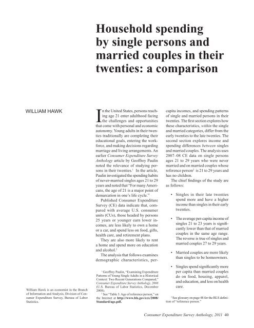
In the United States, persons reaching
age 21 enter adulthood facing
the challenges and opportunities
that come with personal and economic
autonomy. Young adults in their twenties
traditionally are completing their
educational goals, entering the workforce,
and making decisions regarding
marriage and living arrangements. An
earlier Consumer Expenditure Survey
Anthology article by Geoffrey Paulin
noted the relevance of studying persons
in their twenties. 1 In the article,
Paulin investigated the spending habits
of never-married singles ages 21 to 29
years and noted that “For many Americans,
the age of 21 is a major point of
demarcation in one’s life cycle.”
Published Consumer Expenditure
Survey (CE) data indicate that, compared
with average U.S. consumer
units (CUs), those headed by persons
25 years or younger earn lower incomes,
are less likely to own a home
or a car, and spend less on food, gifts,
health care, and retirement plans.
They are also more likely to rent
a home and spend more on education
and alcohol. 2
The analysis that follows examines
demographic characteristics, per-
1 Geoffrey Paulin, “Examining Expenditure
Patterns of Young Single Adults in a Historical
Context: Two Recent Generations Compared,”
Consumer Expenditure Survey Anthology, 2008
(U.S. Bureau of Labor Statistics, December
2008).
2 See “Table 3. Age of reference person,” on
the Internet at http://www.bls.gov/cex/2008/
Standard/age.pdf.
capita incomes, and spending patterns
of single and married persons in their
twenties. The first section explores how
these characteristics, within the single
and married categories, differ from the
early twenties to the late twenties. The
second section explores income and
spending differences between singles
and married couples. The analysis uses
2007–08 CE data on single persons
ages 21 to 29 years who were never
married and on married couples whose
reference person 3 is 21 to 29 years and
has no children.
The chief findings of the study are
as follows:
• Singles in their late twenties
spend more and have a higher
income than singles in their early
twenties.
• The average per-capita income of
singles 21 to 23 years is significantly
lower than that of married
couples in the same age range.
The reverse is true of singles and
married couples 27 to 29 years.
• Married couples are more likely
than singles to be homeowners.
• Singles spend significantly more
per capita than married couples
do on food, housing, apparel,
and education, and less on health
care.
3 See glossary on page 48 for the BLS definition
of “reference person.”
Consumer Expenditure Survey Anthology, 2011 40

Data and methods
Interview survey. The data for this article
are from the 2007–08 Interview
Survey component of the CE. The Interview
Survey contains information
on incomes, expenditures, and demographic
characteristics of American
consumers, collected quarterly from
a nationally representative sample of
CUs in the U.S. population.
The CE includes two components:
the quarterly Interview Survey and
the weekly Diary Survey. Published
CE tables are created by integrating
information from the two surveys.
The Interview Survey, which is designed
to collect data on major types
of expenditures, household characteristics,
and income, is used in this study
because it provides the most complete
picture of spending. Respondents are
usually asked to report values for
expenditures or outlays that occurred
during the three months prior to the
interview. The data in this analysis
are by collection year, not calendar
year, from CUs interviewed in 2007
and 2008. This study employs many
of the methods set forth in Paulin’s
article.
Outlays. The analysis that follows
uses outlays, as opposed to expenditures,
for comparisons. Outlays are
similar to expenditures in that both
measures (1) define spending as the
transaction cost, including taxes, to
obtain goods and services, (2) include
spending on gifts for people outside
of the CU, and (3) exclude business
expenses. The key difference is in
the treatment of purchases of real
property and vehicles. In the CE, expenditures
on purchases of property
include only mortgage interest and
expenditures on vehicles include the
full value of the purchased vehicle,
regardless of whether it was or was
not financed. By contrast, outlays
include both the principal and interest
portions of property on mortgages
and vehicle loans. The purchase price
of vehicles bought outright and not
financed also is included in outlays.
Weights. The CE uses a representative
sample to estimate the spending habits
of the U.S. civilian noninstitutional
population. Estimates shown in this
article are calculated with the use of
weights. For the 2007–08 Interview
Survey, approximately 600 married
CUs and 2,200 single CUs provided
data for this analysis. These sampled
CUs represent nearly 7 million CUs
in the population.
Reference groups. Recognizing that
21- to 29-year-olds are not a homogeneous
group and that the twenties
are a period of lifestyle transition,
the analysis examines three distinct
groups: those CUs (with reference
person) ages 21 to 23 years, those in
their midtwenties (24 to 26 years),
and those in their late twenties (27 to
29 years). Further restrictions on the
age difference between spouses in a
married-couple CU follow.
Consumers must be single or married
with no children in order to be
included in the analysis. To be categorized
as a “single” CU, a person must
identify him- or herself as single and
never married and must be in a CU
of size 1. This categorization implies
that the person is not living with
other blood relatives, is not widowed
or divorced, and, if there are other
people living in the housing unit, is
financially independent (that is, is
not making joint financial decisions
with his or her housemates). Financial
independence is determined by
the three major expense categories:
housing, food, and other living expenses.
To be considered financially
independent, the respondent must
pay all or part of the consumer unit’s
expenses in at least two of the three
major expense categories.
Examples of singles eligible for
this study include a 25-year-old living
with three of her friends who
makes her own financial decisions
and a 21-year-old residing in a college
dormitory even if he receives
money from his parents each month.
In contrast, a 27-year-old living at
home with his parents is not counted
as single even if he is financially
independent.
For the married group, each CU
must, of course, be married and must
be living in a two-member CU. In
order to allow for closer comparisons
between singles and couples in the
same age group, couples with age differences
greater than 4 years between
their members are omitted from their
respective groups.
An example of a married couple
eligible for the study is a married
couple, one member of whom is age
27, and the other age 31, with no
children. The same couple would be
eligible even if the pair rented out
their basement to another family. By
contrast, any couple whose members
Groups eligible to participate in the study
Single
Ages: 21–23; 24–26; 27–29
CU type: single persons
CU size: 1
Marital status: single, never married
Married
Age of reference person: 21–23; 24–26; 27–29
Age of spouse: within 4 years of age of reference person
CU type: husband and wife only
CU size: 2
Marital status: married, no children
Consumer Expenditure Survey Anthology, 2011 41

are, respectively, 22 and 27 years
would not be eligible, because their
ages differ by more than 4 years.
Also ineligible is a couple living in
the home of the reference person’s
parents, regardless of the members’
ages and financial independence.
Results are from the eligibility classification
used and were computed on
a per-capita basis, unless explicitly
stated otherwise. This approach allows
for closer comparisons between singles
and couples.
Early twenties compared with
late twenties
Singles. Sixty-seven percent of singles
in their early twenties (21 to 23 years)
are enrolled in college either full or
part time, 18 percent have earned a
bachelor’s degree, and 6 percent report
owning a home. (See chart 1.)
Singles in their early twenties
tend to spend more money, on average,
than they earn per year. Table 1
shows that average reported outlays
of 21- to 23-year-olds exceed average
income by about $5,000 ($21,083 and
$16,067).
Lending credence to the view that
singles in their twenties are in a transitional
period, more of those in their
late twenties have bought a home or
earned a bachelor’s degree. Thirty-five
percent of singles ages 27 to 29 years
report owning a home, 55 percent have
earned a bachelor’s degree, and 18
percent are enrolled in college either
part time or full time.
The average income of a late-twenties
single, $39,757, is almost 2½ times
that of an early-twenties single, and the
average total outlay of a late-twenties
single, $34,889, is well above that of
an early-twenties single. Late-twenties
singles outspend early-twenties singles
in every expenditure category except
education.
There are also differences in how
singles allocate their outlays. Earlytwenties
singles spend a larger share
of their budgets on food and education
and a smaller share on housing and
transportation than do late-twenties
singles. Food accounts for 18.0 per-
cent, and education 11.0 percent, of
outlays for an early-twenties single,
whereas food accounts for only 14.6
percent, and education 1.6 percent,
for a late-twenties single. Housing
accounts for 34.5 percent, and transportation
14.2 percent, of outlays for an
early-twenties single; housing makes
up 39.0 percent, and transportation
16.6 percent, of outlays for a latetwenties
single.
Married couples. For married CUs
with reference person ages 21 to 23
years, 17 percent report owning a
home, 21 percent have at least one
person with a bachelor’s degree, and
46 percent have at least one person
enrolled in college either part or full
time. (See chart 2.) Average per-capita
income is $22,986 and average percapita
total outlays are $20,120. (See
table 1.)
The twenties are also a transitional
age for couples. Of married couples
with reference person ages 27 to 29
years, 69 percent report owning their
home, 73 percent live in a CU with
at least one person with a bachelor’s
degree, and 29 percent are CUs with at
least one member enrolled in college
either part or full time. The average
per-capita income of the late-twenties
married group, $38,182, is 66 percent
higher than the average per-capita
income of the early-twenties married
group, whereas average per-capita
total outlays of late-twenties married
couples, $26,649, are 32 percent higher
than those of early-twenties married
couples.
Early-twenties couples spend a
larger share of their budgets on food,
transportation, and entertainment, and
a smaller share on housing, than do
late-twenties couples. Food accounts
for 15.4 percent, transportation 21.3
percent, and entertainment 6.5 percent
of total outlays for an early-twenties
couple, whereas food accounts for 13.6
percent, transportation 19.5 percent,
and entertainment 5.4 percent for a
late-twenties couple. Housing constitutes
30.0 percent of outlays for an
early-twenties couple, compared with
35.6 percent for a late-twenties couple.
Singles compared with married
couples
Demographics. For the combined
single and married-couple groups
ages 21 to 29 years, married couples
are far more likely than singles to be
homeowners. The statistics show that
55 percent of married couples report
owning their homes and 84 percent of
singles are renters. Sixty-one percent
of married CUs and 39 percent of
single CUs, have at least one member
with a bachelor’s degree, and 39 percent
of married CUs, compared with 43
percent of single CUs have at least one
member currently enrolled in college.
The difference in home ownership
rates of singles and married couples is
the smallest for 21- to 23-year-olds,
compared with 27- to 29-year-olds. For
the younger group, 6 percent of singles
and 17 percent of couples report home
ownership.
The difference in home ownership
rates is the largest among 27- to 29-yearolds,
with 69 percent of married couples
reporting home ownership, compared
with 35 percent of singles.
For the 21- to 23-year-olds, 67
percent of singles report that they are
enrolled in college and 46 percent
of couples report having at least one
member enrolled in college. Also, 18
percent of singles have a bachelor’s
degree, and 21 percent of married
persons have at least one member
with a bachelor’s degree. For the 27-
to 29-year-olds, 18 percent of singles
report that they are enrolled in college
and 29 percent of married persons
report having at least one member
enrolled in college. Fifty-five percent
of singles have a bachelor’s degree
or higher, and 73 percent of married
couples have at least one member with
a bachelor’s degree or higher.
Income. Married couples ages 21 to
29 have incomes that are, on average,
$6,779 more than singles’ incomes.
Among singles, average income is
$16,067 for 21- to 23-year-olds, compared
with $39,757 for 27- to 29-yearolds.
(See chart 3.) Among married
couples, income averages $22,986 for
Consumer Expenditure Survey Anthology, 2011 42

the younger age group, compared with
$38,182 for older married couples. Differences
in income between singles and
married couples are largest in the early
twenties ($6,919) and smallest in the
late twenties ($1,575).
Singles in their late twenties with at
least a bachelor’s degree or higher earn
$42,645, and those in their late twenties
with a high school diploma or less
earn $26,708. Married couples in their
late twenties with at least one member
with a bachelor’s degree or higher earn
$40,240 per capita, and late-twenties
married couples for which the highest
level attained by either member
is a high school diploma or less earn
$33,169 per capita.
Outlays. For all CUs, ages 21 to 29,
average outlays are similar for singles
and married couples, with the latter
spending $1,532 less. Differences
in outlays between singles and married
couples are smallest in the early
twenties ($963) and largest in the late
twenties ($8,240). (See chart 4.)
Spending patterns. For the three age
groups combined, singles spend 6
percent more per capita than married
couples spend, but married couples
earn 25 percent more per capita in
income than singles earn. Income and
total outlays, however, tell only part of
the story; a focus on how outlays are
allocated demonstrates the differences
in spending patterns of single and married
consumers.
For all age groups combined, singles
spend a larger share of their budget
on food, housing, and education, and a
smaller share on transportation and on
personal insurance and pensions, than
do married couples. Specifically, food
accounts for 16.3 percent, housing 36.7
percent, and education 5.7 percent of
total outlays for singles, whereas food
accounts for 13.1 percent, housing
34.5 percent, and education 2.4 percent
for married couples. Transportation
makes up 15.6 percent, and personal
insurance and pensions 8.9 percent, of
total outlays for singles; transportation
accounts for 20.0 percent, and personal
insurance and pensions 12.7 percent,
for married couples.
For each age group, some of the
differences in spending shares between
singles and married couples are
more pronounced than for the three
age groups combined. Among 21- to
23-year-olds, singles and married
couples allocate their spending quite
differently: singles apportion a higher
percentage of their outlays to food, alcohol,
housing, and education, whereas
married couples apportion a higher
percentage of their outlays to transportation,
health care, and entertainment.
The same result holds for the 27- to
29-year age group; however, for most
areas of spending, the difference is
smaller. Singles’ and married couples’
budget shares for food, alcohol, housing,
transportation, health care, entertainment,
and education are closer to
each other in the 27- to 29-year age
group than in the 21- to 23-year age
group. In this regard, late-twenties
singles resemble late-twenties couples
more than they resemble early-twenties
singles.
Summary of total outlays
Data from the Interview Survey component
of the CE for 2007–08 show
that ages 21 to 29 years are a time of
transition for young adults. Regardless
of their marital status, persons in their
late twenties, ages 27 to 29 years, earn
more, spend more, are more likely to
have a bachelor’s degree, and are more
likely to own a home than are their earlytwenties
counterparts. Singles in their
early twenties earn less in income than
early-twenties married couples, but spend
about the same amount per capita. However,
late-twenties singles earn per-capita
incomes similar to those of late-twenties
married couples, but spend significantly
more per capita. Finally, late-twenties
singles report larger per-capita outlays
than married couples do in each category
examined, except for health care.
Consumer Expenditure Survey Anthology, 2011 43

Table 1. Characteristics, per-capita outlays, and outlay shares of singles and married couples, by age group,
2007–08
21–29 years 21–23 years 24–26 years 27–29 years
Category
Single
Married
couple
Single
Married
couple
Single
Married
couple
Single
Married
couple
Number of CUs (in thousands) 5,236 1,515 2,083 243 1,737 578 1,417 694
Per-capita income $27,267 $34,046 $16,067 $22,986 $30,512 $33,723 $39,757 $38,182
Percent distribution:
Sex
Men 58 50 56 50 59 50 60 50
Women
Housing tenure
42 50 44 50 41 50 40 50
Homeowner 16 55 6 17 14 55 35 69
Renter
Educational status (highest level
attained by single or by any
member of married couple)
84 45 94 83 86 45 65 31
High school diploma or less 61 39 82 79 50 36 45 27
Bachelor’s degree or higher
College enrollment (by single or by
either member of married couple)
39 61 18 21 50 64 55 73
Enrolled 43 39 67 46 34 47 18 29
Not enrolled 57 61 33 54 66 53 82 71
Total per-capita outlays: $27,178 $25,646 $21,083 $20,120 $28,197 $26,761 $34,889 $26,649
Food 4,417 3,363 3,798 3,101 4,592 3,173 5,111 3,613
Food at home 2,359 1,940 2,050 1,932 2,417 1,830 2,744 2,036
Food away from home 2,057 1,423 1,748 1,169 2,175 1,343 2,367 1,577
Alcoholic beverages 660 227 637 195 683 265 668 205
Housing 9,964 8,844 7,266 6,045 10,238 9,249 13,593 9,484
Apparel 896 650 760 596 827 774 1,180 567
Transportation 4,233 5,128 2,991 4,286 4,461 5,393 5,779 5,202
Health care 570 963 334 913 663 1,061 802 899
Entertainment 1,346 1,347 1,048 1,299 1,415 1,246 1,702 1,448
Education 1,544 611 2,329 731 1,405 737 560 464
Personal insurance and pensions 2,431 3,250 1,200 1,932 2,782 3,279 3,811 3,686
Other outlays1 1,117 1,264 720 1,021 1,131 1,585 1,683 1,081
Total outlay shares (percent)
Food 16.3 13.1 18.0 15.4 16.3 11.9 14.6 13.6
Food at home 8.7 7.6 9.7 9.6 8.6 6.8 7.9 7.6
Food away from home 7.6 5.5 8.3 5.8 7.7 5.0 6.8 5.9
Alcoholic beverages 2.4 0.9 3.0 1.0 2.4 1.0 1.9 0.8
Housing 36.7 34.5 34.5 30.0 36.3 34.6 39.0 35.6
Apparel 3.3 2.5 3.6 3.0 2.9 2.9 3.4 2.1
Transportation 15.6 20.0 14.2 21.3 15.8 20.2 16.6 19.5
Health care 2.1 3.8 1.6 4.5 2.4 4.0 2.3 3.4
Entertainment 5.0 5.3 5.0 6.5 5.0 4.7 4.9 5.4
Education 5.7 2.4 11.0 3.6 5.0 2.8 1.6 1.7
Personal insurance and pensions 8.9 12.7 5.7 9.6 9.9 12.3 10.9 13.8
Other outlays1 4.1 4.9 3.4 5.1 4.0 5.9 4.8 4.1
1 Other outlays include personal care, reading, tobacco, cash contributions, and miscellaneous.
Source: U.S. Bureau of Labor Statistics, Consumer Expenditure Survey, 2007–08
Consumer Expenditure Survey Anthology, 2011 44

Percent
80
70
60
50
40
30
20
10
0
50
40
30
20
10
Chart 1. Comparison of home ownership, attainment of bachelor’s degree, and
college enrollment by singles in their early twenties and late twenties, 2007–08
Singles, 21 to 23
Singles, 27 to 29
Homeowner Bachelor's degree Enrolled in college
Source: U.S. Bureau of Labor Statistics, Consumer Expenditure Survey, 2007–08
Percent
80
Chart 2. Comparison of home ownership, attainment of bachelor’s degree, and
college enrollment, by age of married reference person, 2007–08
Percent Percent
80
80
Married, 21 to 23
70
70
Married, 27 to 29
60
60
0
Homeowner Bachelor's degree Enrolled in college
0
Source: U.S. Bureau of Labor Statistics, Consumer Expenditure Survey, 2007–08
Consumer Expenditure Survey Anthology, 2011 45
70
60
50
40
30
20
10
0
50
40
30
20
10

Income
(dollars)
45,000
40,000
35,000
30,000
25,000
20,000
15,000
Outlays
40,000
35,000
30,000
25,000
20,000
15,000
Chart 3. Income of single persons and of married couples ages 21–29, 2007–08
Married couples
Single persons
Early twenties Midtwenties Late twenties
Source: U.S. Bureau of Labor Statistics, Consumer Expenditure Survey, 2007–08
Chart 4. Outlays of single persons and of married couples ages 21–29, 2007–08
Married couples
Single persons
Early twenties Midtwenties Late twenties
Source: U.S. Bureau of Labor Statistics, Consumer Expenditure Survey, 2007–08
Income
(dollars)
45,000
40,000
35,000
30,000
25,000
20,000
15,000
Outlays
40,000
35,000
30,000
25,000
20,000
15,000
Consumer Expenditure Survey Anthology, 2011 46