AIR Tools - A MATLAB Package for Algebraic Iterative ...
AIR Tools - A MATLAB Package for Algebraic Iterative ...
AIR Tools - A MATLAB Package for Algebraic Iterative ...

You also want an ePaper? Increase the reach of your titles
YUMPU automatically turns print PDFs into web optimized ePapers that Google loves.
<strong>AIR</strong> <strong>Tools</strong> - A <strong>MATLAB</strong> <strong>Package</strong><br />
<strong>for</strong> <strong>Algebraic</strong> <strong>Iterative</strong><br />
Reconstruction Techniques<br />
Maria Saxild-Hansen<br />
Kongens Lyngby 2010
Technical University of Denmark<br />
In<strong>for</strong>matics and Mathematical Modelling<br />
Building 321, DK-2800 Kongens Lyngby, Denmark<br />
Phone +45 45253351, Fax +45 45882673<br />
reception@imm.dtu.dk<br />
www.imm.dtu.dk
Summary<br />
In this master thesis a <strong>MATLAB</strong> package <strong>AIR</strong> <strong>Tools</strong> with implementations of<br />
several iterative algebraic reconstruction methods <strong>for</strong> discretizations of tomography<br />
problems is developed. The focus is mainly on the two classes of methods:<br />
Simultaneous <strong>Iterative</strong> Reconstruction Technique (SIRT) and <strong>Algebraic</strong> Reconstruction<br />
Techniques (ART). The package also includes three simplified test<br />
problems from medical and seismic tomography.<br />
For each iterative method a number of strategies <strong>for</strong> choosing the relaxation<br />
parameter and the stopping rule are presented and implemented. The relaxation<br />
parameter can be chosen as a fixed parameter or chosen adaptively in each<br />
iteration. For the fixed case a training strategy is developed <strong>for</strong> finding the<br />
optimal parameter <strong>for</strong> a given test problem. The stopping rules provided in the<br />
package is the Discrepancy Principle, the Monotone Error Rule and the NCP<br />
criterion. For the first two methods a training strategy is also provided <strong>for</strong><br />
finding an optimal stopping parameter.<br />
In addition simulation studies and comparisons of per<strong>for</strong>mance of the available<br />
methods and strategies are presented and discussed.<br />
This thesis also includes manual pages <strong>for</strong> each implemented routine that describes<br />
the use of the implemented routines.<br />
KEYWORDS: ART methods, SIRT methods, iterative methods, semi-convergence,<br />
relaxation parameters, stopping rules, tomography.
Resumé<br />
I dette eksamensprojekt udvikles en <strong>MATLAB</strong> programpakke, <strong>AIR</strong> <strong>Tools</strong>, med<br />
implementeringer af flere iterative algebraiske rekonstruktions metoder til diskretiseret<br />
tomografi problemer. Det primære fokus er p˚a to klasser af metoder: Simulatan<br />
<strong>Iterative</strong> Rekonstruktion Teknik (SIRT) og Algebraiske Rekonstruktions<br />
Teknikker (ART). Programpakken indeholder ligeledes tre simple testproblemer<br />
fra medicinsk og seismisk tomografi.<br />
For hver iterative metode præsenteres og implementeres en række strategier til<br />
at vælge relaxations parameteren samt stopkriterier. Relaxations parameteren<br />
kan enten vælges som en konstant parameter eller den kan vælges adaptivt i<br />
hver iteration. For det konstante tilfælde er der udviklet en træningsstrategi<br />
til at finde den optimale værdi <strong>for</strong> et givent testproblem. Stopkriterierne, der<br />
er tilgængelige i denne pakke, er discrepancy princippet, monotone error reglen<br />
samt NCP kriteriet. For de to første metoder er der givet en træningsstrategi<br />
til at finde den optimale værdi <strong>for</strong> stopparamerten.<br />
Yderligere er studier og sammenligninger af metodernes og strategiernes opførsel<br />
ogs˚a præsenteret of diskuteret.<br />
Eksamensprojektet indeholder ogs˚a manual sider til hver implementeret funktion,<br />
som beskriver benyttelsen heraf.<br />
STIKORD: ART metoder, SIRT metoder, iterative metoder, semi-konvergens,<br />
relaxation parameter, stopkriterier, tomografi.
Preface<br />
This master thesis is prepared at the Department of In<strong>for</strong>matics and Mathematical<br />
Modeling, Technical University of Denmark (DTU), and marks the<br />
completion of the master degree in Mathematical Modeling and Computations.<br />
It represents the workload of 35 ETCS points and has been prepared during a<br />
seven month period from August 31 to March 31. The study has been conducted<br />
under the supervision of Professor Per Christian Hansen.<br />
I would like to thank a few people <strong>for</strong> helping me with this project. I would like<br />
to thank Professor in scientific compution at University of Linköping, Dept. of<br />
Mathematics, Tommy Elfving who, through a visit at DTU in November 2009<br />
provided valuable insight into the theory of iterative methods. I would also like<br />
to thank Professor at DTU In<strong>for</strong>matics Klaus Mosegaard <strong>for</strong> his assistance in<br />
creation of a seismic tomography problem and a usefull test phantom and Ph.D.<br />
student Jakob Heide Jørgensen <strong>for</strong> assistance in creation an algorithm <strong>for</strong> the<br />
tomography test problems. Finally, I would like to thank my family and friends,<br />
especially Katrine Lange and Elin A. Larsen <strong>for</strong> assistance and <strong>for</strong> keeping up<br />
my spirit.<br />
Kgs. Lyngby, 31th March 2010<br />
Maria Saxild-Hansen
List of Symbols<br />
The following is a list of symbols used over the thesis. Be aware that this list<br />
only contains the symbols which are used <strong>for</strong> the same purpose through the<br />
thesis. This list is there<strong>for</strong>e not a complete list since only frequently used symbols<br />
are represented. Also be aware that some symbols have multiple meanings.<br />
However the meaning will be clear from the context.<br />
Symbol Quantity Dimension<br />
A coefficient matrix m × n<br />
ai i’th row in the matrix A m<br />
aj j’th column in the matrix A m<br />
aij element in the i’th row and the j’th column of A scalar<br />
b<br />
¯b right-hand side<br />
exact right-hand side<br />
m<br />
m<br />
bi i’th element in the vector b scalar<br />
δ the noise level scalar<br />
I identity matrix<br />
k iteration number scalar<br />
λk relaxation parameter k or scalar<br />
M symmetric, positive definite matrix <strong>for</strong> the SIRT m × m<br />
methods<br />
m, n matrix dimensions scalars<br />
Φ k (σ, λ) iteration-error scalar<br />
ϕi filter factor scalar<br />
Φ diagonal matrix of filter factors n × n
viii Contents<br />
̟ average number of nonzero elements in a row scalar<br />
Ψk (σ, λ) noise-error scalar<br />
ρ spectral radius scalar<br />
Σ diagonal matrix with all singular values m × n<br />
σi singular value of matrix scalar<br />
the number of nonzero elements in the j’th col- scalar<br />
sj<br />
umn<br />
τ the stopping parameter scalar<br />
τ1 parameter <strong>for</strong> the modified Ψ1-based relaxation scalar<br />
τ2 parameter <strong>for</strong> the modified Ψ2-based relaxation scalar<br />
T symmetric positive definite matrix <strong>for</strong> the SIRT n × n<br />
methods<br />
U matrix with all left singular vectors m × m<br />
ui i’th left singular vector m<br />
V matrix with all right singular vectors n × n<br />
vi i’th right singular vector n<br />
w weighting vector m<br />
wi i’th element in the weighting vector scalar<br />
x k solution in the k’th iteration n<br />
¯x exact solution n<br />
Hi the i’th hyperplane<br />
Pi(·) projection<br />
Ri(·) reflection<br />
〈·, ·〉 inner product, i.e. 〈x, y〉 = xTy. · 2 2-norm<br />
NNZ(·) number of nonzero elements scalar
Contents<br />
Summary i<br />
Resumé iii<br />
Preface v<br />
List of Symbols vii<br />
List of Figures xiv<br />
1 Introduction 1<br />
1.1 Sturcture of the Thesis . . . . . . . . . . . . . . . . . . . . . . . . 2<br />
2 Theory of Inverse Problems and Regularization 5<br />
2.1 Discrete Ill-Posed Problems . . . . . . . . . . . . . . . . . . . . . 5<br />
2.2 SVD and Picard Condition . . . . . . . . . . . . . . . . . . . . . 6<br />
2.3 Spectral Filtering . . . . . . . . . . . . . . . . . . . . . . . . . . . 9<br />
2.4 <strong>Iterative</strong> Methods and Semi-Convergence . . . . . . . . . . . . . 10<br />
2.5 Resolution Limit . . . . . . . . . . . . . . . . . . . . . . . . . . . 11<br />
3 <strong>Iterative</strong> Methods <strong>for</strong> Reconstruction 13<br />
3.1 Simultaneous <strong>Iterative</strong> Reconstructive Technique (SIRT) . . . . . 14<br />
3.2 <strong>Algebraic</strong> Reconstruction Techniques (ART) . . . . . . . . . . . . 21<br />
3.3 Considerations Towards the <strong>Package</strong> . . . . . . . . . . . . . . . . 26<br />
3.4 Block-<strong>Iterative</strong> Methods . . . . . . . . . . . . . . . . . . . . . . . 27<br />
4 Semi-Convergence and Choice of Relaxation Parameter 33<br />
4.1 Semi-Convergence <strong>for</strong> SIRT Methods . . . . . . . . . . . . . . . . 33<br />
4.2 Choice of Relaxation Parameter . . . . . . . . . . . . . . . . . . . 38
x CONTENTS<br />
5 Stopping Rules 53<br />
5.1 Stopping Rules with Training . . . . . . . . . . . . . . . . . . . . 53<br />
5.2 Normalized Cumulative Periodogram . . . . . . . . . . . . . . . . 58<br />
6 Test Problems 61<br />
7 Testing the Methods 67<br />
7.1 Convergence of DROP . . . . . . . . . . . . . . . . . . . . . . . . 69<br />
7.2 Symmetric Kaczmarz as a SIRT Method . . . . . . . . . . . . . . 70<br />
7.3 Test of the Choice of Relaxation Parameter . . . . . . . . . . . . 71<br />
7.4 Stopping Rules . . . . . . . . . . . . . . . . . . . . . . . . . . . . 83<br />
7.5 Relaxation Strategies Combined with Stopping Rules . . . . . . . 89<br />
8 Manual Pages 97<br />
9 Conclusion and Future Work 147<br />
9.1 Future Work . . . . . . . . . . . . . . . . . . . . . . . . . . . . . 148<br />
A Appendix 149<br />
A.1 Orthogonal Projection on a Hyperplane . . . . . . . . . . . . . . 149<br />
A.2 Investigation of the Roots . . . . . . . . . . . . . . . . . . . . . . 152<br />
A.3 Work Units <strong>for</strong> the SIRT and ART methods . . . . . . . . . . . . 154<br />
Bibliography 155
List of Figures<br />
2.1 SVD basis . . . . . . . . . . . . . . . . . . . . . . . . . . . . . . . 7<br />
2.2 Picard plot . . . . . . . . . . . . . . . . . . . . . . . . . . . . . . 7<br />
2.3 Illustration of basis semi-convergence . . . . . . . . . . . . . . . . 10<br />
3.1 Cimmino’s reflection method . . . . . . . . . . . . . . . . . . . . 16<br />
3.2 Cimmino’s projection method . . . . . . . . . . . . . . . . . . . . 18<br />
3.3 Kaczmarz’s method . . . . . . . . . . . . . . . . . . . . . . . . . 22<br />
3.4 Symmetric Kaczmarz . . . . . . . . . . . . . . . . . . . . . . . . . 23<br />
4.1 Behaviour of Φ k (σ, λ) and Ψ k (σ, λ). . . . . . . . . . . . . . . . . 37<br />
4.2 Ψ k (σ, λ) as function of σ . . . . . . . . . . . . . . . . . . . . . . . 39<br />
4.3 Relative error histories <strong>for</strong> nine values of λ . . . . . . . . . . . . . 40<br />
4.4 The minimum relative errors <strong>for</strong> different λ-values . . . . . . . . 40<br />
4.5 Optimal number of iterations <strong>for</strong> a SIRT method . . . . . . . . . 41
xii LIST OF FIGURES<br />
4.6 Relative error histories <strong>for</strong> an ART method . . . . . . . . . . . . 43<br />
4.7 The minimum relative errors <strong>for</strong> different λ-values <strong>for</strong> an ART<br />
method . . . . . . . . . . . . . . . . . . . . . . . . . . . . . . . . 44<br />
4.8 Optimal number of iterations <strong>for</strong> an ART method . . . . . . . . . 44<br />
4.9 Relative error histories <strong>for</strong> a SIRT method with maximum number<br />
of iterations. . . . . . . . . . . . . . . . . . . . . . . . . . . . 46<br />
4.10 Minimum relative error <strong>for</strong> a SIRT method with maximum number<br />
of iterations. . . . . . . . . . . . . . . . . . . . . . . . . . . . 46<br />
4.11 Optimal number of iterations <strong>for</strong> a SIRT method with maximum<br />
number of iterations . . . . . . . . . . . . . . . . . . . . . . . . . 47<br />
4.12 Illustration of line search . . . . . . . . . . . . . . . . . . . . . . . 48<br />
6.1 Parallel beam illustration . . . . . . . . . . . . . . . . . . . . . . 62<br />
6.2 Fan beam illustration . . . . . . . . . . . . . . . . . . . . . . . . 63<br />
6.3 Seismic tomography illustration . . . . . . . . . . . . . . . . . . . 64<br />
6.4 The two exact phantoms . . . . . . . . . . . . . . . . . . . . . . . 65<br />
7.1 Relative error histories <strong>for</strong> test of DROP . . . . . . . . . . . . . . 68<br />
7.2 Relative error histories <strong>for</strong> test of DROP using weighting . . . . 69<br />
7.3 Ψ-based relaxations <strong>for</strong> symmetric Kaczmarz . . . . . . . . . . . 71<br />
7.4 Training of relaxation parameter using Cimmino’s projection method 72<br />
7.5 Training of relaxation parameter using Kaczmarz’s method . . . 72<br />
7.6 Training of relaxation parameter using randomized Kaczmarz . . 73<br />
7.7 Relative errors <strong>for</strong> the SIRT methods with trained λ . . . . . . . 73<br />
7.8 Relative errors <strong>for</strong> the ART methods with trained λ . . . . . . . 74
LIST OF FIGURES xiii<br />
7.9 Training of relaxation parameter using Cimmino’s projection method<br />
with maximum number of iterations . . . . . . . . . . . . . . . . 76<br />
7.10 Training of relaxation parameter using Kaczmarz’s method with<br />
maximum number of iterations . . . . . . . . . . . . . . . . . . . 76<br />
7.11 Training of relaxation parameter using randomized Kaczmarz<br />
method with maximum number of iterations . . . . . . . . . . . . 77<br />
7.12 Relative error <strong>for</strong> the SIRT methods using line search . . . . . . 78<br />
7.13 Relative error using the Ψ-based relaxations . . . . . . . . . . . . 79<br />
7.14 Relative error using the modified Ψ-based relaxations . . . . . . 79<br />
7.15 Relative errors <strong>for</strong> the SNARK test problem with different relaxation<br />
strategies . . . . . . . . . . . . . . . . . . . . . . . . . . . . 81<br />
7.16 Training of stopping rule <strong>for</strong> Cimmino’s projection method . . . 84<br />
7.17 Training of stopping rule <strong>for</strong> DROP . . . . . . . . . . . . . . . . 84<br />
7.18 Training of stopping rule <strong>for</strong> Kaczmarz’s method . . . . . . . . . 85<br />
7.19 Illustration of the stopping rules <strong>for</strong> the SIRT methods . . . . . . 86<br />
7.20 Illustration of the stopping rules <strong>for</strong> the ART methods . . . . . . 87<br />
7.21 Ψ-based relaxation with stopping rules . . . . . . . . . . . . . . . 90<br />
7.22 Line search with stopping rules . . . . . . . . . . . . . . . . . . . 91<br />
7.23 Training λ with stopping rules <strong>for</strong> SIRT methods . . . . . . . . . 93<br />
7.24 Training λ with stopping rules <strong>for</strong> ART methods . . . . . . . . . 94<br />
A.1 Illustration of projection on hyperplane where origo is in the hyperplane<br />
. . . . . . . . . . . . . . . . . . . . . . . . . . . . . . . . 150<br />
A.2 Illustration of projection on the hyperplane wheer origo is not in<br />
the hyperplane . . . . . . . . . . . . . . . . . . . . . . . . . . . . 151<br />
A.3 Illustration of the roots . . . . . . . . . . . . . . . . . . . . . . . 152
xiv<br />
A.4 Zoom of the roots . . . . . . . . . . . . . . . . . . . . . . . . . . 153
Chapter 1<br />
Introduction<br />
In the beginning of the 20th century the Polish mathematician Stefan Kaczmarz<br />
[27] and the Italian mathematician Gianfranco Cimmino [8] independently developed<br />
iterative algorithms <strong>for</strong> solving linear systems. In 1970 Gordon, Bender<br />
and Herman rediscovered Kaczmarz’s method applied in medical imaging [17].<br />
They called the method ART (<strong>Algebraic</strong> Reconstruction Technique) and when<br />
Houndsfield patented the first CT-scanner in 1972, which awarded him together<br />
with Cormark the Nobel Prize in 1979, the classical methods found their practical<br />
purpose in tomograpgy [24]. The word tomography means reconstruction<br />
from slices. After the invention of the CT-scanner several new methods familiar<br />
with the old classical methods were developed.<br />
This master thesis deals with the classical Kaczmarz’s and Cimmino’s methods<br />
but also with the methods familiar with these methods. We divide the gathered<br />
methods into two main categories, the SIRT and the ART methods, and present<br />
strategies <strong>for</strong> choosing the relaxation parameter and different stopping rules.<br />
We will compare the per<strong>for</strong>mance of different methods and different strategies<br />
on a test problem derived from medical tomography.
2 Introduction<br />
1.1 Sturcture of the Thesis<br />
The goal of the project is to develope and implement a <strong>MATLAB</strong> package containing<br />
a number of iterative methods <strong>for</strong> algebraic reconstruction used in tomography<br />
problems. This includes describing the methods in a common framework<br />
such that the methods are described in same notation and the created<br />
functions have similar interfaces. Furthermore strategies <strong>for</strong> choosing the relaxation<br />
parameter must be availiable just as different stopping rules must be<br />
included. A few test problems relevant <strong>for</strong> these kind of methods must also<br />
be implemented. A critical comparison of the different methods and strategies<br />
used on different test problems will be produced. Finally the thesis will have<br />
the <strong>for</strong>m as a extended manual such that it contains chapters with theory and<br />
manual pages <strong>for</strong> each implemented routine.<br />
The chapters of the thesis are organized in the following way:<br />
• Chapter 2: We begin by giving a short presentation of inverse problem<br />
theory and defining the concept of semi-convergence <strong>for</strong> iterative methods<br />
and the concept of resolution limit.<br />
• Chapter 3: In this chapter we introduce the theory of the gathered SIRT<br />
and ART methods which this package concerns. We also provide a brief<br />
overview of block-iterative methods.<br />
• Chapter 4: In the next chapter we examine the semi-convergence behaviour<br />
of a part of the SIRT methods. After this examination we introduce<br />
different strategies of choosing the relaxation parameter, where one<br />
of the strategies is based on the examination of semi-convergence.<br />
• Chapter 5: In this chapter we introduce three strategies <strong>for</strong> the stopping<br />
rules. To devise effective stopping rules a training strategy is introduced<br />
<strong>for</strong> two of the stopping rules.<br />
• Chapter 6: We introduce in this chapter three different test problems,<br />
where two of the test problems arise from medical tomography and the<br />
third test problem arise from seismic tomography.<br />
• Chapter 7: This chapter discusses the per<strong>for</strong>mance of the methods. We<br />
also examine the perfomance of the methods when the different strategies<br />
<strong>for</strong> choosing the relaxation parameter and <strong>for</strong> different stopping rules are<br />
used. Furthermore we compare the per<strong>for</strong>mance of the SIRT and the ART<br />
methods.
1.1 Sturcture of the Thesis 3<br />
• Chapter 8: This chapter contains an overview of the implemented routines<br />
followed by an individual manual page <strong>for</strong> each function in the package.<br />
The manual pages are arranged alphabetically.<br />
• Chapter 9: This chapter contains the conclusion and suggenstions <strong>for</strong><br />
future work.<br />
All the implemented <strong>MATLAB</strong> routines have been implemented in <strong>MATLAB</strong><br />
7.8. To produce the test results, examples and figures a large number of scrips<br />
have been created but only the relevant functions are included in the package.
4 Introduction
Chapter 2<br />
Theory of Inverse Problems<br />
and Regularization<br />
Inverse problems arise in many applications in science and technology. Examples<br />
where inverse problems are found could be in medical imaging, where it is used<br />
e.g. in CT scanning, in geophysical prospecting or image deblurring. We will in<br />
this chapter introduce some of the fundamental concepts of inverse problems.<br />
We will first introduce the concept of an inverse problem and describe what<br />
defines an ill-posed problem. Then the important tools of SVD and the discrete<br />
Picard condition is defined followed by a few examples of spectral filtering.<br />
Finally we will give a short description of semi-convergence <strong>for</strong> iterative methods<br />
and define the concept of resolution limit.<br />
2.1 Discrete Ill-Posed Problems<br />
Inverse problems arise when we need to compute in<strong>for</strong>mation that is either<br />
internal or hidden. In the <strong>for</strong>ward problem we have a known input and a known<br />
system and we can then compute the output. In the inverse problem the output<br />
is often known with errors and we then have to compute either the system or<br />
the input, where the other one is known. For the linear problems we let the<br />
system be represented by the matrix A ∈ R m×n , the output as the right-hand
6 Theory of Inverse Problems and Regularization<br />
side b ∈ R m , which is the known data and the solution x ∈ R n . The problem<br />
can be <strong>for</strong>mulated as a system of linear equations:<br />
Ax = b, (2.1)<br />
where the matrix A typically is a discretization from an ill-posed problem, e.g.<br />
the Radon trans<strong>for</strong>m. The system (2.1) is said to be overdetermined when<br />
m > n and underdetermined when m < n.<br />
The definition of a well-posed problem was invented by Hadamard, who stated<br />
that a problem is well-posed if it satisfies the following requirements:<br />
Existence: There exist a solution to the problem.<br />
Uniqueness: There exist only one solution to the problem.<br />
Stability: The solution must depend continuously on data.<br />
If one of the three conditions is not satisfied, then the problem is said to be<br />
ill-posed.<br />
2.2 SVD and Picard Condition<br />
An important tool in analysing inverse problems is the singular value decomposition<br />
(SVD). SVD is defined <strong>for</strong> any matrix A ∈ R m×n as<br />
A =<br />
min{m,n} <br />
i=1<br />
uiσiv T i ,<br />
where the vectors ui and vi are orthonormal, and<br />
σ1 ≥ σ2 ≥ · · · ≥ σ min{m,n} ≥ 0.<br />
The elements σi are the singular values and the rank of the matrix A is equal<br />
to the number of positive singular values. Assuming that the inverse of A exists<br />
it is given as<br />
A −1 =<br />
min{m,n} <br />
i=1<br />
1<br />
viu<br />
σi<br />
T i .
2.2 SVD and Picard Condition 7<br />
U(:,k)<br />
U(:,k)<br />
U(:,k)<br />
0<br />
−0.2<br />
k = 1<br />
−0.4<br />
0 50<br />
n<br />
k = 4<br />
0.5<br />
0<br />
−0.5<br />
0 50<br />
n<br />
k = 7<br />
0.5<br />
0<br />
−0.5<br />
0 50<br />
n<br />
U(:,k)<br />
U(:,k)<br />
U(:,k)<br />
0.5<br />
0<br />
k = 2<br />
−0.5<br />
0 50<br />
n<br />
k = 5<br />
0.5<br />
0<br />
−0.5<br />
0 50<br />
n<br />
k = 8<br />
0.5<br />
0<br />
−0.5<br />
0 50<br />
n<br />
U(:,k)<br />
U(:,k)<br />
U(:,k)<br />
0.5<br />
0<br />
k = 3<br />
−0.5<br />
0 50<br />
n<br />
k = 6<br />
0.5<br />
0<br />
−0.5<br />
0 50<br />
n<br />
k = 9<br />
0.5<br />
0<br />
−0.5<br />
0 50<br />
n<br />
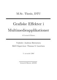
Figure 2.1: The first 9 left singular vectors ui <strong>for</strong> the test problem shaw.<br />
10 5<br />
10 0<br />
10 −5<br />
10 −10<br />
10 −15<br />
Picard Plot with b exact<br />
σ<br />
i<br />
T<br />
|u b|<br />
i<br />
T<br />
|u b|/σi<br />
i<br />
10<br />
0 10 20 30 40 50<br />
−20<br />
i<br />
(a) Picard plot with no noise.<br />
10 20<br />
10 10<br />
10 0<br />
10 −10<br />
Picard Plot with b noise<br />
σ<br />
i<br />
T<br />
|u b|<br />
i<br />
T<br />
|u b|/σi<br />
i<br />
10<br />
0 10 20 30 40 50<br />
−20<br />
i<br />
(b) Picard plot with noise.<br />
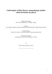
Figure 2.2: The Picard plot <strong>for</strong> the test problem shaw. The left figure is with no noise<br />
while the right figure is with noise level δ = 10 −3 .
8 Theory of Inverse Problems and Regularization<br />
Using this we can write the naive solution as<br />
x = A −1 b =<br />
min{m,n} <br />
i=1<br />
Figure 2.1 shows the first nine left singular vectors ui <strong>for</strong> the test problem shaw<br />
from Regularization <strong>Tools</strong> [21] with white noise level δ = 10 −3 . We see that<br />
the singular vectors have more oscillations as i increases, and the corresponding<br />
singular values σi decrease.<br />
We will now investigate the behaviour of the SVD coefficients 〈ui, b〉 and 〈ui,b〉<br />
. σi<br />
We call a plot of these coefficients together a Picard plot. Figure 2.2 shows the<br />
Picard plot <strong>for</strong> the test problem shaw with n = 50. From the left plot (a) we see<br />
the Picard plot when no noise is added to the right-hand side. We notice that the<br />
SVD coefficients |〈ui, b〉| decay faster than the singular values σi. This continues<br />
until i ≥ 18 where the coefficients level off. We recognize the reached level as the<br />
machine precision. We also notice that the solution coefficients 〈ui,b〉<br />
also decay<br />
σi<br />
but <strong>for</strong> i ≥ 18 they increase due to the inaccuracy of the coefficients 〈ui, b〉.<br />
We there<strong>for</strong>e cannot expect to get a meaningful solution to the inverse problem<br />
since the influence of the rounding errors destroys the computed solution.<br />
The plot to the right (b) shows the same problem, but we have used a noisy<br />
right-hand side. In this plot the SVD coefficients |〈ui, b〉| also decay until a<br />
certain level where they level off. This level is determined by the added noise.<br />
Also the solution’s coefficients 〈ui,b〉<br />
decay in the beginning, but increase again<br />
σi<br />
when the SVD coefficients |〈ui, b〉| level off. In this case the computed solution<br />
is totally dominated by the SVD coefficients which corresponds to the smaller<br />
singular values.<br />
u T i b<br />
In this connection we introduce the discrete Picard Condition.<br />
Definition 2.1 (Discrete Picard Condition) The discrete Picard Condition<br />
is satisfied if <strong>for</strong> all singular values σi greater than τ the corresponding coefficients<br />
|〈ui, b〉| on average decay faster than σi, where τ denotes the level at<br />
which the computed singular values level off due to rounding errors.<br />
Notice that the Picard Condition is about the decay and not the size of the<br />
singular values and the coefficients |〈ui, b〉|. If the discrete Picard condition is<br />
not satisfied then we cannot expect to solve a discrete ill-posed problem.<br />
σi<br />
vi.
2.3 Spectral Filtering 9<br />
2.3 Spectral Filtering<br />
Due to the difficulties associated with the discrete inverse problems the naive<br />
solution x = A −1 b is useless since it is becomes dominated by the rounding<br />
errors. We will in this section introduce two spectral filtering methods, which<br />
can be expressed as a filtered SVD expansion on the <strong>for</strong>m:<br />
xfilter =<br />
min{m,n} <br />
i=1<br />
ϕi<br />
〈ui, b〉<br />
vi,<br />
where ϕi are the filter factors <strong>for</strong> the corresponding method. We will first<br />
introduce the truncated SVD method (TSVD).<br />
We realised that the large errors in the naive solution came from the noisy SVD<br />
coefficients corresponding to the smallest singular values but we also noticed that<br />
the SVD coefficients <strong>for</strong> large singular values were useful, since these coefficients<br />
fulfilled 〈ui,b〉<br />
σi ≃ 〈ui,¯b〉 , where b is the noisy right-hand side and σi<br />
¯b is the righthand<br />
side without noise. This leads to the truncated SVD (TSVD) method<br />
where we choose only to include the first k components of the naive solution<br />
to x. With this method we there<strong>for</strong>e cut off those SVD coefficients that are<br />
dominated by inverted noise. We define the TSVD solution as<br />
xk =<br />
σi<br />
k 〈ui, b〉<br />
vi,<br />
i=1<br />
where we call k the truncation parameter and k must be chosen such that all<br />
the noise-dominated SVD coefficients are discarded. This leads to the following<br />
filter factors <strong>for</strong> the TSVD method:<br />
ϕi =<br />
σi<br />
1 i ≤ k<br />
0 i > k.<br />
The second method we will introduce the Tikhonov regularization. For this<br />
method the filter factors is defined as<br />
ϕi =<br />
σ 2 i<br />
σ 2 i<br />
+ ω2 , i = 1, · · · , n,<br />
where ω is the regularization parameter, which in a sense corresponds to the<br />
truncation parameter k. The Tikhonovs regularization corresponds to the following<br />
minimization problem<br />
min<br />
x {Ax − b 2 2 + ω2 x 2 2 }.
10 Theory of Inverse Problems and Regularization<br />
x 0<br />
x 1<br />
x 2<br />
x k<br />
x k opt<br />
x exact<br />
A −1 b<br />
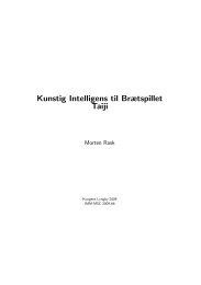
Figure 2.3: The basis concept of semi-convergence<br />
We notice that <strong>for</strong> σi ≫ ω, then the filter factors are close to 1 and the corresponding<br />
SVD components contribute to xfilter with almost full strength. On<br />
the other hand when σi ≪ ω then the filter factors are close to σ 2 i /ω2 , and the<br />
SVD components are damped or filtered.<br />
2.4 <strong>Iterative</strong> Methods and Semi-Convergence<br />
For large problems where it is not feasible to compute the SVD, we need other<br />
methods than the introduced TSVD and Tikhonov regularization. This leads us<br />
to the use of iterative methods, where we need a user-specified starting vector<br />
x 0 , and from this vector the method produces a sequence of iterates x 1 , x 2 , . . .<br />
that converge to some solution.<br />
For iterative methods Natterer [31] has introduced the concept of semi-convergence.<br />
The concept describes the behaviour of the iterate x k <strong>for</strong> the iterative methods.<br />
The first iterates tend to be better and better approximations of the exact solution<br />
but at some point the iterates start to deteriorate and instead they converge<br />
to the naive solution x = A −1 b, see figure 2.3. For the iterative methods the<br />
regularization parameter is there<strong>for</strong>e the number of iterations.
2.5 Resolution Limit 11<br />
2.5 Resolution Limit<br />
When exploring the iterative methods, which this package concerns, we need to<br />
define the concept of resolution limit. For a better understanding of this concept<br />
we draw attention to the fact that the relative error is defined as<br />
xk − ¯x2<br />
,<br />
¯x2<br />
where x k is the solution in the k’th iterate and ¯x is the exact solution.<br />
The bound <strong>for</strong> how accurate a solution one can obtain, is determined by the<br />
noise in the data and this can be studied in terms of the SVD. We then define<br />
the resolution limit to be this bound. The resolution limit is not only dependent<br />
on the noise but also the used method and the given problem to solve. We define<br />
the resolution limit to be<br />
RL(A, b, method) = min<br />
k<br />
xk − ¯x2<br />
.<br />
¯x2<br />
From this definition we let the resolution limit depend on the used method, and<br />
the problem.
12 Theory of Inverse Problems and Regularization
Chapter 3<br />
<strong>Iterative</strong> Methods <strong>for</strong><br />
Reconstruction<br />
In this chapter we will give a brief introduction to the theory <strong>for</strong> some iterative<br />
methods called SIRT and ART methods. The need <strong>for</strong> iterative methods arises,<br />
when the dimensions of the matrix A become so large that direct factorization<br />
methods become infeasible, which is usually the case in two and three dimensions.<br />
This is typically the case when A is a discretization that arises from a<br />
real-world problem. In this case one can use iterative methods instead of the<br />
well-known Tikhonov regularization or TSVD described in section 2.3. Where<br />
we <strong>for</strong> Tikhonov regularization have the regularization parameter ω, the number<br />
of iterations k plays the role of regularization parameter <strong>for</strong> the iterative<br />
methods.<br />
In the following presented theory we will assume that all the elements in the<br />
matrix A are nonnegative. In the articles where the methods are defined they<br />
do not include used-defined weights, but we have chosen to include them in both<br />
the description and the implementation.
14 <strong>Iterative</strong> Methods <strong>for</strong> Reconstruction<br />
3.1 Simultaneous <strong>Iterative</strong> Reconstructive Technique<br />
(SIRT)<br />
In this section we will present the class of iterative methods which we call<br />
Simultaneous <strong>Iterative</strong> Reconstructive Technique (SIRT). As the name refers to,<br />
all the methods of this class are simultaneous, which means that in<strong>for</strong>mation<br />
from all the equations are used at the same time.<br />
In the literature the class of SIRT methods is also referred to as Landwebertypes,<br />
since the Landweber iteration is one of the classical methods of the SIRTclass.<br />
The common property of the SIRT methods is that they can be written<br />
in the following general <strong>for</strong>m:<br />
x k+1 = x k + λkTA T M(b − Ax k ), k = 0, 1, . . . (3.1)<br />
where x k denotes the current iteration vector, x k+1 denotes the new iteration<br />
vector, λk is the relaxation parameter, and the matrices M and T are symmetric<br />
positive definite. We will realize that the different methods depend on the choice<br />
of the matrices M and T. In most of the presented methods we will have that<br />
T = I.<br />
For the methods given on the <strong>for</strong>m (3.1) with T = I the following theorem<br />
regarding convergence has been shown [4], [25].<br />
Theorem 3.1 The iterates on the <strong>for</strong>m (3.1) with T = I converge to a solution<br />
ˆx of Ax − bM if and only if<br />
0 < ǫ ≤ λk ≤ 2<br />
σ2 − ǫ,<br />
1<br />
where ǫ is an arbitrarily small, but fixed constant and σ1 is the largest singular<br />
value of M 1<br />
2 A. If in addition x 0 ∈ R(A T ), then ˆx is the unique solution of<br />
minimum 2-norm.<br />
Theorem 3.1 is a useful theorem since it insures convergence of the SIRT methods<br />
in general. It was originally only proved to be a sufficient condition <strong>for</strong> convergence,<br />
but in [35] it is shown that the condition is also necessary as stated in<br />
the theorem.<br />
3.1.1 Classical Landweber Method<br />
The classical Landweber method was first introduced by Landweber in [29],<br />
and it has often been used <strong>for</strong> image reconstruction. The classical Landweber
3.1 Simultaneous <strong>Iterative</strong> Reconstructive Technique (SIRT) 15<br />
method can be written as follows:<br />
x k+1 = x k + λkA T (b − Ax k ), k = 0, 1, . . ., (3.2)<br />
which corresponds to setting M = T = I in (3.1).<br />
The iterates x k from (3.2) can be expressed as filtered SVD solutions. If we let<br />
the SVD <strong>for</strong> the matrix A take the following <strong>for</strong>m<br />
A = UΣV T =<br />
then the filtered solution can be written as<br />
where Φ k is given as<br />
The filter factors ϕ k i<br />
n<br />
i=1<br />
x k = V Φ k Σ −1 U T b,<br />
uiσiv T i ,<br />
Φ k = diag ϕ k 1, . . . , ϕ k n .<br />
<strong>for</strong> i = 1, . . .,n are given as<br />
ϕ k i = 1 − 1 − λσ 2k i .<br />
For small singular values σi we have that Φk i ≈ kλσ2 i showing that they decay<br />
with the same rate as the Tikhonov filter factors described in section 2.3.<br />
3.1.2 Generalized Landweber<br />
Another classical method is the generalized Landweber iteration which is described<br />
in [20] and [33]. The generalized Landweber has the following <strong>for</strong>m:<br />
x k+1 = x k + λTA T (b − Ax k ), k = 0, 1, . . .,<br />
where λ is our constant relaxation parameter and T is a ”sharping matrix” given<br />
by<br />
T = F(A T A),<br />
where F is a rational function of A T A. We obtain the classical Landweber<br />
method when F = I.<br />
The filter factors ϕ k i<br />
<strong>for</strong> the generalized Landweber method are given by<br />
ϕ k i = 1 − (1 − σ 2 i F(σ 2 i )) k ,
16 <strong>Iterative</strong> Methods <strong>for</strong> Reconstruction<br />
✻ R2<br />
H2<br />
H1<br />
✙<br />
R2(z)<br />
R1(z)<br />
z<br />
✲<br />
Figure 3.1: Cimmino’s reflection method<br />
since the eigenvalue decomposition of F(A T A) is given as<br />
F(A T A) =<br />
n<br />
i=1<br />
viF(σ 2 i )v T i .<br />
We see that using the generalized Landweber method gives a further impact<br />
on the filter factors, since the function F occurs in the filter factors. It is also<br />
possible to choose the function in such a way that the method approximates,<br />
say, the TSVD or the Tikhonov regularization.<br />
3.1.3 Cimmino’s Method<br />
Another method in the SIRT-class is Cimmino’s method which was introduced<br />
in [8]. Cimmino’s method was originally based on reflections onto hyperplans<br />
but there also exists a version with projections.<br />
To introduce the two versions of Cimmino’s method, we define Hi to be the<br />
hyperplanes <strong>for</strong> the linear equations 〈a i , x〉 = bi:<br />
Hi = {x ∈ R n | a i , x = bi}, <strong>for</strong> i = 1, . . .,m.<br />
We will introduce both versions of Cimmino’s method, and we will start with<br />
the original that uses reflections.
3.1 Simultaneous <strong>Iterative</strong> Reconstructive Technique (SIRT) 17<br />
The idea about Cimmino’s reflection method is that the next iterate can be<br />
described using an equal weighting of the reflections of x k on Hi. Reflections<br />
on hyperplanes is the following:<br />
Ri(z) = z + 2 bi − 〈ai , z〉<br />
ai2 a<br />
2<br />
i .<br />
The reflection method then uses the average of the reflections of x k onto the<br />
hyperplanes Hi to determine the direction of the step to the new iteration.<br />
Figure 3.1 illustrates the concept in R 2 <strong>for</strong> a consistent problem. The method<br />
can then be written as follows:<br />
x k+1 = x k + λk<br />
m 1 <br />
wi Ri(x<br />
m<br />
k ) − x k ,<br />
i=1<br />
where the relaxation parameter λk determines how much of the step is taken<br />
from x k to the new iterate x k+1 and wi > 0 are user-defined weights. Using the<br />
definition of reflections we get the following:<br />
x k+1 = x k + λk<br />
m 2<br />
m<br />
i=1<br />
wi<br />
bi − 〈ai , xk 〉<br />
ai2 ai <strong>for</strong> k = 0, 1, . . ..<br />
2<br />
Cimmino’s reflection method can be written using matrix notation on the <strong>for</strong>m<br />
wi<br />
<strong>for</strong> i = 1, . . .,m and T = I.<br />
(3.1), where M = 2<br />
m diag<br />
a i 2 2<br />
We will now introduce Cimmino’s projection method. Using an equal weighting<br />
of all the equations the next iterate in Cimmino’s projection method can be<br />
described using orthogonal projections of x k on Hi. As shown in appendix A.1<br />
an orthogonal projection of the vector z on the hyperplane Hi is the following:<br />
Pi(z) = z + bi − a i , z <br />
a i 2 2<br />
a i . (3.3)<br />
Cimmino’s projection method uses the average of the projections of x k onto the<br />
hyperplanes Hi to determine the direction of the step to the new iterate. Figure<br />
3.2 illustrates the concept in R 2 <strong>for</strong> a consistent problem.<br />
The new iterate can then be described as the current iterate plus a contribution<br />
of the average of the found step direction. We can there<strong>for</strong>e write Cimmino’s<br />
projection method as the following:<br />
x k+1 = x k + λk<br />
1<br />
m<br />
m<br />
i=1<br />
<br />
wi Pi(x k ) − x k ,
18 <strong>Iterative</strong> Methods <strong>for</strong> Reconstruction<br />
✻ R2<br />
H2<br />
H1<br />
P1(z)<br />
✙<br />
P2(z)<br />
z<br />
✲<br />
Figure 3.2: Cimmino’s projection method<br />
where the relaxation parameter λk determines how much of the step is taken<br />
from x k to the new iterate x k+1 and wi are userdefined weights, where wi > 0<br />
<strong>for</strong> i = 1, . . .,m.<br />
Using the definition of orthogonal projection (3.3) we can rewrite the expression:<br />
x k+1 = x k + λk<br />
m 1<br />
m<br />
i=1<br />
wi<br />
bi − ai , xk a i<br />
a i 2 2<br />
<strong>for</strong> k = 0, 1, . . ..<br />
Using matrix notation Cimmino’s projection method has the general <strong>for</strong>m (3.1),<br />
wi<br />
<strong>for</strong> i = 1, 2, . . ., m and T = I.<br />
where M = 1<br />
m diag<br />
a i 2 2<br />
3.1.4 Component Averaging (CAV)<br />
Component Averaging (CAV) is introduced in [6] and is an expansion of Cimmino’s<br />
method. In Cimmino’s method we use equal weighting of the contributions<br />
from the projections. In the case where the matrix A is dense, it seems<br />
fair that all contributions <strong>for</strong> Pi(x k ) − x k are equally weighted.<br />
The heuristic in CAV includes a factor which is proportional to the number of<br />
nonzero elements. We there<strong>for</strong>e let sj denote the number of nonzero elements
3.1 Simultaneous <strong>Iterative</strong> Reconstructive Technique (SIRT) 19<br />
of column j <strong>for</strong> each j = 1, 2, . . ., n:<br />
sj = NNZ(aj), <strong>for</strong> j = 1, . . .,n.<br />
We then define a i 2 S = n<br />
j=1 a2 ij sj. Using this the CAV algorithm is as follows:<br />
x k+1<br />
j<br />
= xk j<br />
+ λk<br />
m<br />
i=1<br />
wi<br />
bi − a i , x k<br />
a i 2 S<br />
where wi > 0 are user-defined weights.<br />
a i j <strong>for</strong> k = 0, 1, . . .,<br />
We see that when A is dense we get the original Cimmino’s method, since sj = m<br />
<strong>for</strong> all j = 1, . . .,n, and we have ai2 1<br />
S = mai2 2.<br />
To rewrite the CAV algorithm in matrix <strong>for</strong>m we define S = diag(s1, s2, . . . , sn),<br />
where the sj-values are defined as described above. We then let<br />
<br />
wi<br />
DS = diag <strong>for</strong> i = 1, . . .,m,<br />
a i 2 S<br />
where a i 2 S = (ai ) T Sa i and the CAV algorithm has the following matrix <strong>for</strong>m<br />
x k+1 = x k + λkA T DS(b − Ax k ),<br />
which we recognize as (3.1) with M = DS and T = I.<br />
3.1.5 Diagonally Relaxed Orthogonal Projections (DROP)<br />
Another method in the SIRT class is the diagonally relaxed orthogonal projection<br />
(DROP) method which is described in [5]. This method is another<br />
extension of Cimmino’s method, which is inspired by the CAV method. In the<br />
DROP method we also introduce a user-defined weighting of the equations. We<br />
let wi > 0 denote this weighting.<br />
The DROP method can then be written as:<br />
m<br />
x k+1 = x k + λk<br />
i=1<br />
wiS −1 (Pi(x k ) − x k ),<br />
where Pi(x k ) is defined as in (3.3) and S is defined as above <strong>for</strong> CAV. Using<br />
(3.3) we can rewrite the DROP algorithm into the following <strong>for</strong>m:<br />
x k+1<br />
j<br />
= xk j<br />
1<br />
+ λk<br />
sj<br />
m<br />
i=1<br />
wi<br />
bi − a i , x <br />
a i 2 2<br />
a i j ,
20 <strong>Iterative</strong> Methods <strong>for</strong> Reconstruction<br />
<strong>for</strong> all j = 1, 2, . . .,n. Recall that wi > 0 <strong>for</strong> all i = 1, . . .,m are user-chosen<br />
weights. When wi = 1 <strong>for</strong> all i = 1, . . .,m and the matrix A is dense, i.e. sj = m<br />
<strong>for</strong> all j = 1, . . . , n then we have Cimmino’s method.<br />
The DROP method has the following matrix <strong>for</strong>m:<br />
x k+1 = x k + λkS −1 A T D(b − Ax k ), (3.4)<br />
which we recognize as the general <strong>for</strong>m with T = S−1 <br />
wi<br />
and M = D = diag ai2 2<br />
Since the DROP method has T = I, we cannot use theorem 3.1 and there<strong>for</strong>e we<br />
make a further investigation of the convergence theory. By defining yk = S 1<br />
2xk 1<br />
and Ā = AS− 2 we can rewrite to another matrix <strong>for</strong>m:<br />
y k+1 = y k + λk ĀT D(b − Āyk ).<br />
For this <strong>for</strong>m it is known, that λk must be between 0 and 2/ρ( ĀTDĀ). Using<br />
the definition of Ā we get that ρ(ĀT DĀ) = ρ(S−1AT DA). Then in [5] it is<br />
shown that <strong>for</strong> the DROP method where wi > 0 <strong>for</strong> all i = 1, . . .,m and if<br />
D = diag wi/ai2 <br />
m×m −1<br />
2 ∈ R and S = diag(1/sj) ∈ Rn×n , where sj = 0,<br />
then ρ(S −1 A T DA) ≤ max{wi|i = 1, . . .,m}. We there<strong>for</strong>e have the following<br />
convergence theorem which replaces theorem 3.1 <strong>for</strong> the DROP method, where<br />
we let zD = 〈z, Dz〉 denote the D-norm:<br />
Theorem 3.2 Assume that wi > 0 <strong>for</strong> all i = 1, . . .,m. If <strong>for</strong> all k ≥ 0,<br />
0 < ǫ ≤ λk ≤ (2 − ǫ)/ max{wi|i = 1, . . .,m},<br />
where ǫ is an arbitrarily small but fixed constant, then any sequence generated by<br />
(3.4) converges to a weighted least squares solution x ∗ = argmin{Ax −bD|x ∈<br />
R n }. If in addition x 0 ∈ R(S −1 A T ), then x ∗ is the unique solution of minimum<br />
S-norm.<br />
3.1.6 Simultaneous <strong>Algebraic</strong> Reconstruction Technique<br />
(SART)<br />
Simultaneous <strong>Algebraic</strong> Reconstruction Technique (SART) is developed in the<br />
ART setting [1], but it can be written in the general SIRT <strong>for</strong>m (3.1) and we<br />
there<strong>for</strong>e categorize it as a SIRT method.<br />
The SART method is written in the following matrix <strong>for</strong>m:<br />
x k+1 = x k + λkV −1 A T W(b − Ax k ),<br />
<br />
.
3.2 <strong>Algebraic</strong> Reconstruction Techniques (ART) 21<br />
where V = diag(ςj) and W = diag 1<br />
ςi <br />
i , where ς and ςj denotes the row and<br />
the column sums:<br />
ς i =<br />
ςj =<br />
n<br />
j=1<br />
m<br />
i=1<br />
a i j<br />
a i j<br />
<strong>for</strong> i = 1, . . .,m<br />
<strong>for</strong> j = 1, . . .,n.<br />
For this method we assume that ai = 0 and aj = 0, such that A does not contain<br />
any zero rows or columns.<br />
Since the SART method has T = I, we cannot use theorem 3.1. The convergence<br />
<strong>for</strong> SART was independently developed by Censor, Elfvind in [4] and Jiang,<br />
Wang in [26]. Both showed that the convergence <strong>for</strong> SART is within the interval<br />
(0, 2).<br />
3.2 <strong>Algebraic</strong> Reconstruction Techniques (ART)<br />
We now introduce a different class of methods which we will denote algebraic<br />
reconstruction techniques (ART). All methods in the ART-class are fully sequential<br />
method, i.e., each equation is treated at a time, since each equation is<br />
dependent on the previous.<br />
3.2.1 Kaczmarz’s Method<br />
The classical and most known method of the ART class is called Kaczmarz’s<br />
method, [27]. The method is a so-called row action method, since each iteration<br />
consist of a ”sweep” through all the rows in the matrix A. Since the method uses<br />
one equation in each step, an iteration consists of m steps. Figure 3.3 shows<br />
an example of a sweep <strong>for</strong> the consistent case with the relaxation parameter<br />
λk = 1.<br />
The algorithm <strong>for</strong> Kaczmarz’s method updates x k in the following way:<br />
x k,0 = x k ,<br />
x k,i = x k,i−1 bi −<br />
+ λk<br />
ai , xk,i−1 ai2 2<br />
x k+1 = x k,m .<br />
a i , i = 1, 2, . . .,m,
22 <strong>Iterative</strong> Methods <strong>for</strong> Reconstruction<br />
H4<br />
H5<br />
H3<br />
H2<br />
H6<br />
H1<br />
x k+1<br />
x k<br />
Figure 3.3: Kaczmarz’s Method<br />
If the linear system (2.1) is consistent, then Kaczmarz’s method converges to a<br />
solution of this system. If the system is inconsistent, then every sub-sequence<br />
of iterations converges, but not necessarily to a least squares solution.<br />
In the literature Kaczmarz’s method is also referred to as ART, which can be<br />
confusing since ART is also the name of algebraic reconstruction techniques in<br />
general.<br />
Experiments have shown that Kaczmarz’s method converges fast in the first<br />
iterations after which it converges very slowly. This is perhaps one of the reasons<br />
why this method was often used <strong>for</strong> tomography problems, where the solution<br />
is often found within few iterations.<br />
By using SOR-theory it can be shown that Kaczmarz’s method <strong>for</strong> λ constant<br />
in each iteration can by written in the <strong>for</strong>m (3.1), but then MA is no longer<br />
symmetric [13]:<br />
x k+1 = x k + λA T MA(b − Ax k ), (3.5)<br />
where MA = (D + λL) −1 . Since MA is not symmetric, we cannot use the<br />
theory derived <strong>for</strong> the SIRT-methods. It can on the other hand be proved, that<br />
<strong>for</strong> 0 < λ < 2, then the iterations of Kaczmarz’s method (3.5) converge to a
3.2 <strong>Algebraic</strong> Reconstruction Techniques (ART) 23<br />
solution of<br />
H4<br />
H5<br />
H3<br />
H2<br />
H6<br />
H1<br />
x k+1<br />
x k<br />
Figure 3.4: Symmetric Kaczmarz<br />
A T MA(b − Ax) = 0.<br />
3.2.2 Symmetric Kaczmarz<br />
A variant of the Kaczmarz method is symmetric Kaczmarz. This method is also<br />
fully sequential, and it consists of one ”sweep” of the Kaczmarz method followed<br />
by another ”sweep” of Kaczmarz’s method, where the equations are used in<br />
reverse order. The iteration <strong>for</strong> the symmetric Kaczmarz method there<strong>for</strong>e<br />
consists of 2m − 2 steps. Figure 3.4 shows an example of an iteration <strong>for</strong> the<br />
consistent case with the relaxation parameter λk = 1.<br />
The algorithm <strong>for</strong> symmetric Kaczmarz method is the following:<br />
x k,0 = x k<br />
x k,i = x k,i−1 bi −<br />
+ λk<br />
ai , xk,i−1 ai2 2<br />
x k+1 = x k,1 ,<br />
where x k,1 denotes the last of the step in (3.6).<br />
a i , i = 1, . . .,m, . . . ,2 (3.6)
24 <strong>Iterative</strong> Methods <strong>for</strong> Reconstruction<br />
Symmetric Kaczmarz was introduced in [3] and as <strong>for</strong> the Kaczmarz’s method<br />
symmetric Kaczmarz can also be rewritten to have the <strong>for</strong>m of the SIRT methods<br />
[14], where λk = λ:<br />
x k+1 = x k + λA T MSA(b − Ax k ),<br />
where MSA is symmetric, which means that the theory <strong>for</strong> SIRT methods is<br />
valid, but not practical to implement in this way.<br />
3.2.3 Randomized Kaczmarz<br />
The next method we will introduce is the randomized Kaczmarz method. Experience<br />
has shown that Kaczmarz’s method converges very slowly to the solution.<br />
The method we present was proposed in [36] and is proved to have exponential<br />
expected rate of convergence, and the rate does not depend on the number of<br />
equations in the system. The randomized Kaczmarz method has the following<br />
<strong>for</strong>m:<br />
x k+1 = x k + br(i) − ar(i) , xk ar(i) 2 a<br />
2<br />
r(i) ,<br />
where the index r(i) is chosen from the set {1, 2, . . ., m} randomly with probability<br />
proportional with a r(i) 2 2 .<br />
For the randomized Kaczmarz method we cannot talk about iterations but only<br />
the number of steps.<br />
In the definition of randomized Kaczmarz method in [36] the method is presented<br />
without a relaxation parameter λk, but in our implemented algorithm<br />
this relaxation parameter is present.. We emphasize that no convergence results<br />
exist <strong>for</strong> this parameter and a safe choice would there<strong>for</strong>e be λk = 1, since we<br />
then have the originally presented method.<br />
3.2.4 Extended Kaczmarz Method<br />
As mentioned earlier Kaczmarz’s method cannot provide a least squares solution<br />
in the inconsistent case and there<strong>for</strong>e an extended Kaczmarz method was<br />
proposed. In this method we also consider the orthogonal projections onto the<br />
hyperplanes with respect to the columns of A. We let aj denote the j’th column<br />
of A. The extended Kaczmarz method is given both in a version with and without<br />
relaxation parameters. We will in this section only consider the version with
3.2 <strong>Algebraic</strong> Reconstruction Techniques (ART) 25<br />
relaxation parameters. We again let λ denote the constant relaxation parameter<br />
of the orthogonal projection <strong>for</strong> the rows of A and we let α denote the constant<br />
relaxation parameter <strong>for</strong> the orthogonal projection using the columns.<br />
The extended Kaczmarz method has the following algorithm, where x 0 ∈ R n<br />
and y 0 = b:<br />
y k,0 = y k<br />
y k,j = y k,j−1 − α<br />
y k+1 = y k,n<br />
b k+1 = b − y k+1<br />
x k,0 = x k<br />
aj, y k,j−1<br />
aj 2 2<br />
aj<br />
j = 1, . . .,n<br />
x k,i = x k,i−1 + λ bk+1 − ai , xk,i−1 a i , i = 1, . . . , m<br />
x k+1 = x k,m .<br />
a i 2 2<br />
For the extended Kaczmarz method it is proven in [34] that <strong>for</strong> any x 0 ∈ R n<br />
and <strong>for</strong> any λ, α ∈ (0, 2) the method converges to a least squares solution. This<br />
method is not implemented in the package.<br />
3.2.5 Multiplicative ART<br />
Another method in the ART class is the multiplicative ART method. This<br />
method was proposed by in [17]. For this method we assume that x 0 is a n<br />
dimensional vector of all ones and that all the elements in A are between 0 and<br />
1, 0 ≤ aij ≤ 1. The multiplicative ART method is given as:<br />
x k+1<br />
j<br />
=<br />
<br />
bi<br />
〈ai , xk aij x<br />
〉<br />
k j,<br />
where i = (k mod m) + 1. Originally when the method was presented is was<br />
assumed that all the elements in A are either 0 or 1, but later is has been shown<br />
that if<br />
• all the entries of A are between 0 and 1<br />
• A does not have zero rows<br />
• the system (2.1) has a nonnegative solution
26 <strong>Iterative</strong> Methods <strong>for</strong> Reconstruction<br />
Work Units WU<br />
Landweber 2<br />
Cimmino 2<br />
CAV 2<br />
DROP 2<br />
SART 2<br />
Kaczmarz 4<br />
Symmetric Kaczmarz 8<br />
Randomized Kacmarz 4<br />
Table 3.1: Working units <strong>for</strong> one iteration of the SIRT and the ART methods.<br />
then multiplicative ART converges to the maximum entropy of the solution<br />
Ax = b, which is defined as<br />
maxent(x) = −<br />
where ¯x is the average value of xj.<br />
n<br />
j=1<br />
xj xj<br />
ln<br />
n¯x n¯x ,<br />
3.3 Considerations Towards the <strong>Package</strong><br />
We have now introduced some SIRT and ART methods. For the package we will<br />
only use some of the introduced methods. For the methods, which are left out of<br />
the package we found them interesting, such that they should be described and<br />
mentioned. In the package we will use the SIRT methods Landweber, Cimmino<br />
(both the reflection and the projection version), CAV, DROP and SART. We<br />
have not implemented generalized Landweber, since there is no specific description<br />
of the T matrix. For the ART methods we have implemented Kaczmarz’s<br />
method, symmetric Kaczmarz and randomized Kaczmarz. Extended Kaczmarz<br />
is not implemented, since it requires a choice of two relaxation parameters. The<br />
method MART is also left out of the package, since the algorithm <strong>for</strong> MART is<br />
very different from the other methods.<br />
We have two classes of methods which cannot be directly compared with respect<br />
to computational work, since they have different properties. There<strong>for</strong>e<br />
we introduce the concept of a work unit WU. We define a work unit to be one<br />
matrix-vector multiplication. In appendix A.3 the total work units per iteration<br />
is calculated <strong>for</strong> each of the implemented methods. The result is collected in<br />
table 3.1. We notice that all SIRT methods use 2 WU per iteration, while both<br />
Kaczmarz’s method and randomized Kaczmarz use 4 WU per iteration, since
3.4 Block-<strong>Iterative</strong> Methods 27<br />
we denote one iteration of randomized Kaczmarz to be m random selections<br />
of a row. Since symmetric Kaczmarz uses twice as many steps per iteration<br />
as Kaczmarz’s method the work units per iteration <strong>for</strong> the method is 8. This<br />
result will be used later to compare the per<strong>for</strong>mance of the SIRT and the ART<br />
methods.<br />
When comparing the methods imnplemented in this package, the user should<br />
notice that due to the <strong>MATLAB</strong> implementation the SIRT methods are much<br />
faster than the ART methods. The user should also be aware that this is only the<br />
case since the implementation is done in <strong>MATLAB</strong>, where loops are slow. Using<br />
another language there would not be this difference in the running time. When<br />
implementing the SIRT methods in <strong>MATLAB</strong> a dilemma occurs between speed<br />
and memory. When creating the matrices M and T we have mostly chosen<br />
the fastest implementation but in case of memory trouble most of the SIRT<br />
methods also have an alternative implementation which require less memory<br />
but with a slower running time. If the alternative code exists it can be found in<br />
the comments in the code.<br />
In the following chapters it might seem to the user that we prefer the SIRT<br />
methods, since most of the remaining theory is <strong>for</strong> the SIRT methods, but this<br />
is only the case since a corresponding theory cannot be found <strong>for</strong> the ART<br />
methods.<br />
3.4 Block-<strong>Iterative</strong> Methods<br />
We will now look into the field of block-iterative methods although they are<br />
not a part of this package. The idea of this class of methods is to partition the<br />
system (2.1) into so-called blocks of equations and treat each block according<br />
to the given iterative method by passing cyclic over all the blocks. Most of the<br />
theory <strong>for</strong> block-iterative methods is based on the assumption that equations<br />
can appear in more than one block, but in the following we will always look<br />
at the case with disjoint partitioning, i.e. every equation can only appear in<br />
exactly one block.<br />
For the case of disjoint partitioning we have the following structure of the system:<br />
⎛<br />
⎜<br />
A = ⎜<br />
⎝<br />
A1<br />
A2<br />
.<br />
.<br />
Ap<br />
⎞<br />
⎛<br />
⎟ ⎜<br />
⎟ ⎜<br />
⎟ , b = ⎜<br />
⎠ ⎝<br />
b1<br />
b2<br />
.<br />
.<br />
bp<br />
⎞<br />
⎛<br />
⎟<br />
⎠ , AT ⎜<br />
= ⎜<br />
⎝<br />
B1<br />
B2<br />
.<br />
.<br />
Bq<br />
⎞<br />
⎟<br />
⎠ ,
28 <strong>Iterative</strong> Methods <strong>for</strong> Reconstruction<br />
where p denotes the number of blocks <strong>for</strong> the linear system and q denotes the<br />
number of blocks <strong>for</strong> A T .<br />
For t = 1, . . .,p we let the block with the index Bt ⊆ {1, . . .,m} be a ordered<br />
subset of the <strong>for</strong>m<br />
<br />
Bt = i t 1, i t 2, . . .,i t <br />
m(t) ,<br />
where m(t) is the number of elements in Bt.<br />
We will now introduce some block-iterative methods, but since this software<br />
package does not include block-iterative methods, we will only look at a small<br />
selection. Other block-iterative methods can be found in <strong>for</strong> example [34], [18].<br />
3.4.1 Block-Iteration<br />
The first block-iterative method we will introduce is called the Block-Iteration.<br />
This method was first proposed by Elfving and later generalized by Eggermont,<br />
Herman and Lent. The method is also known as the ordinary Block-Kaczmarz<br />
method. For x 0 ∈ R the algorithm can be written as:<br />
x k,0 = x k<br />
x k,t = x k,t−1 + λtA T t Mt(b t − Atx k,t−1 ), t = 1, 2, . . ., p<br />
x k+1 = x k,p ,<br />
where λt is a set of relaxation parameters and Mt is a set of given symmetric<br />
positive definite matrices. In the algorithm originally proposed by Elfving we<br />
had that Mt = (AtA T t )−1 and λt = λ.<br />
For p = 1, i.e. only one block we have that the method is given on the standard<br />
SIRT <strong>for</strong>m (3.1) with T = I and this is called a fully simultaneous iteration.<br />
With p = m we on the other hand have a fully sequential iteration since each<br />
block consists of only one equation.<br />
In [14] it is proven that if<br />
0 < ǫ ≤ λt ≤<br />
ρ(A T t<br />
2 − ǫ<br />
,<br />
MtAt)<br />
<strong>for</strong> t = 1, . . .,p, then the Block-Iteration method converges.<br />
One block-iteration is defined as a pass through all data and since the Block-<br />
Iteration method uses a single block in each block-step every block-iteration
3.4 Block-<strong>Iterative</strong> Methods 29<br />
consists of p steps. One block-iteration of the Block-Iteration with the relaxation<br />
parameter λk can be written as:<br />
x k+1 = x k + A T ¯ MB(b − Ax k ), (3.7)<br />
¯MB = ( ¯ D + L) −1<br />
where ¯ D is block-diagonal and L is block-lower triangular and defined as:<br />
⎛<br />
0<br />
⎜<br />
L = ⎜ A2A<br />
⎜<br />
⎝<br />
0<br />
T 1<br />
.<br />
. ..<br />
. .. . ..<br />
⎞<br />
⎟<br />
⎠ ,<br />
⎛<br />
λ<br />
D ¯ ⎜<br />
= ⎝<br />
−1 −1<br />
1 M1 . ..<br />
0<br />
ApA T 1 · · · ApA T p−1 0<br />
The sequence defined by (3.7) converges towards the solution of<br />
A T ¯ MB(b − Ax) = 0.<br />
3.4.2 Symmetric Block-Iteration<br />
0 λ−1 p M −1<br />
p<br />
⎞<br />
⎟<br />
⎠ .(3.8)<br />
In Symmetric Block-Iteration one block-iteration consists of first one blockiteration<br />
of the above Block-Iteration method followed by another block-iteration,<br />
where the blocks appear in reverse order. This gives the algorithm the following<br />
control order t = 1, 2, . . .,p − 1, p, p − 1, . . . 1.<br />
The algorithm <strong>for</strong> the symmetric block-iteration <strong>for</strong> x 0 ∈ R n looks as follows:<br />
x k,0 = x k<br />
x k,t = x k,t−1 + λtA T t Mt(b t − Atx k,t−1 ), (3.9)<br />
x k+1 = x k,1 ,<br />
where t = 1, . . .,p − 1, p, p − 1, . . .,1 and x k,1 denotes the last step in (3.9).<br />
One block-iteration of the Symmetric Block-Iteration method can be written in<br />
a general <strong>for</strong>m, where we let<br />
AA T = L + D + L T<br />
be the splitting of AA T into its lower block triangular, block diagonal and upper<br />
block triangular parts. The block-iteration can then be written as:<br />
x k+1 = x k + A T ¯ MSB(b − Ax k ). (3.10)
30 <strong>Iterative</strong> Methods <strong>for</strong> Reconstruction<br />
Using (3.8) and ˜ D = 2 ¯ D − D we get<br />
¯MSB = ( ¯ D + L T ) −1 ˜ D( ¯ D + L) −1 ,<br />
where ¯ MSB is symmetric positive definite.<br />
From [14] we have that the block-iterations of Symmetric Block-Iteration (3.10)<br />
converge to a solution x of the weighted least squares problem<br />
min<br />
x Ax − b ¯ MSB .<br />
If in addition x 0 ∈ R(A T ), then x is the unique solution of minimal 2-norm,<br />
where the corresponding normal equations are<br />
A T ¯ MSB(b − Ax) = 0.<br />
3.4.3 Block-<strong>Iterative</strong> Component Averaging Methods (BI-<br />
CAV)<br />
Earlier we defined the CAV method as one of the SIRT methods. The Block-<br />
<strong>Iterative</strong> Component Averaging method (BICAV) is the block version of the<br />
CAV method introduced in [7]. As <strong>for</strong> the CAV method we will define the<br />
factor s t j . In the BICAV case st j<br />
is the number of nonzero elements in the j’th<br />
column of At <strong>for</strong> t = 1, 2, . . .,p. The BICAV method can then be written on<br />
the following <strong>for</strong>m:<br />
x k+1<br />
j<br />
= xk j + λk<br />
where ai t(k) 2S = n j=1 st(k)<br />
us to the following matrix <strong>for</strong>m:<br />
<br />
i∈B t(k)<br />
bi − ai , xk a i j,<br />
a i t(k) 2 S<br />
j (a i j )2 , t(k) = (k mod p) + 1 and k ≥ 0. This lead<br />
x k+1 = x k + λkA T t(k) M t(k)(b t(k) − A t(k)x k ), (3.11)<br />
<br />
where M = diag 1/ai t(k) 2 <br />
S <strong>for</strong> all i = 1, . . .,m.<br />
In [4] the following convergence theorem is proven <strong>for</strong> the BICAV method:<br />
Theorem 3.3 For<br />
0 < ǫ ≤ λk ≤ (2 − ǫ)/ρ(A T t(k) M t(k)A t(k)),
3.4 Block-<strong>Iterative</strong> Methods 31<br />
where ǫ is an arbitrarily small but fixed constant and M t(k) are given symmetric<br />
and positive definite matrices with the control t(k), then any sequence generated<br />
by (3.11) converges to a solution <strong>for</strong> (2.1). If in addition x 0 ∈ R(A T ), then x k<br />
converges to the solution of minimum 2-norm.<br />
The BICAV method has the property that <strong>for</strong> p = 1 the method becomes fully<br />
simultaneous, i.e. it becomes the CAV method. For p = m we on the other<br />
hand have that BICAV becomes the well-known Kaczmarz’s method.<br />
3.4.4 Block-<strong>Iterative</strong> Diagonally Relaxed Orthogonal Projections<br />
(BIDROP)<br />
For the general SIRT methods we described a method called DROP and we<br />
will now introduce its block-iterative generalization, which we will call Block-<br />
<strong>Iterative</strong> Diagonally Relaxed Orthogonal Projections (BIDROP).<br />
If we let Wt be positive definite diagonal matrices and Ut be symmetric positive<br />
definite matrices <strong>for</strong> t = 1, 2, . . ., p, then the algorithm <strong>for</strong> the BIDROP method<br />
looks as follows:<br />
x k+1 = x k + λkU t(k)A T t(k) W t(k)(b t(k) − Atkx k ), (3.12)<br />
where t(k) = (k mod p) + 1.<br />
The following convergence theorem is derived <strong>for</strong> the BIDROP method:<br />
Theorem 3.4 Let U be a given symmetric and positive definite matrix, and let<br />
Wt be given positive definite diagonal matrices. If <strong>for</strong> all k ≥ 0,<br />
0 < ǫ ≤ λk ≤ (2 − ǫ)/ρ(UA T t(k) W t(k)A t(k)),<br />
where ǫ is an arbitrarily small but fixed constant, then any sequence generated<br />
by (3.12) converges to a solution. If in addition x 0 ∈ R(UA T ), then the solution<br />
has minimal U −1 -norm.<br />
With only one block, i.e. p = 1, and U1 = S and W1 = W, then we have the<br />
standard DROP method.<br />
The BIDROP method is a general method since Ut and Wt is not specific given.<br />
One of the variants of BIDROP is introduced in [5] and is called BIDROP1.
32 <strong>Iterative</strong> Methods <strong>for</strong> Reconstruction<br />
This method has the following scheme:<br />
x k+1 = x k + λkU<br />
where µ t(k)<br />
q is defined as<br />
µ t(k)<br />
q<br />
m(t(k)) <br />
q=1<br />
=<br />
w t(k)<br />
q = 1<br />
µ t(k)<br />
<br />
q b t(k) − a iq it(k) q , x k<br />
a it(k) q ,<br />
w t(k)<br />
q<br />
a it(k)<br />
q 2 2<br />
, where<br />
<strong>for</strong> q = 1, 2, . . .,m(t). The matrix U is fixed <strong>for</strong> each block, i.e. Ut = U and is<br />
given as<br />
<br />
1<br />
U = diag ,<br />
τj<br />
where τj = max st j |t = 1, . . .,p and st j is the number of nonzero elements in<br />
column j <strong>for</strong> the block At.
Chapter 4<br />
Semi-Convergence and Choice<br />
of Relaxation Parameter<br />
4.1 Semi-Convergence <strong>for</strong> SIRT Methods<br />
For the SIRT methods on the <strong>for</strong>m (3.1) with T = I, theorem 3.1 ensures the<br />
convergence to a solution of the least squares problem Ax − bM, but when<br />
solving linear ill-posed problems with iterative methods we are typically more<br />
interested in the earlier mentioned semi-convergence behaviour. We will now<br />
take a close look at the semi-convergence <strong>for</strong> the SIRT methods [16]. To make<br />
the presentation simpler we assume that m ≥ n, but the used theory can be<br />
applied regardless the dimensions.<br />
We assume that the noise in the right-hand side is additive i.e.,<br />
b = ¯ b + δb,<br />
where ¯ b is the noise-free right-hand side and δb is the noise component which<br />
can be caused by discretization errors and measurement errors.<br />
We want to analyze the semi-convergence behaviour of the SIRT scheme where<br />
T = I. To do this we assume that the relaxation parameter λ is constant <strong>for</strong> all<br />
iterations. For convenience we introduce<br />
B = A T MA and c = A T Mb,
34 Semi-Convergence and Choice of Relaxation Parameter<br />
and let the singular value decomposition (SVD) of M 1<br />
2A be<br />
M 1<br />
2A = UΣV T ,<br />
where Σ = diag(σ1, . . . , σp, 0, . . .,0) with σ1 ≥ σ2 ≥ . . . ≥ σp > 0, and<br />
rank(A) = p.<br />
From the SIRT scheme we get the following:<br />
x k = x k−1 + λA T M(b − Ax k−1 )<br />
= x k−1 + λA T Mb − λA T MAx k−1<br />
= x k−1 + λc − λBx k−1<br />
= (I − λB)x k−1 + λc.<br />
By direct insertion we obtain, <strong>for</strong> k = 1,<br />
Similar we <strong>for</strong> k = 2 get:<br />
Similar we <strong>for</strong> k = 3 get:<br />
x 1 = (I − λB)x 0 + λc.<br />
x 2 = (I − λB)x 1 + λc<br />
x 3 = (I − λB)x 2 + λc<br />
= (I − λB) (I − λB)x 0 + λc + λc<br />
= (I − λB) 2 x 0 + (I − λB)λc + λc<br />
= (I − λB) 2 x 0 + ((I − λB) + I) λc.<br />
= (I − λB) (I − λB) 2 x 0 + ((I − λB) + I)λc + λc<br />
= (I − λB) 3 x 0 + (I − λB) 2 + (I − λB) λc + λc<br />
= (I − λB) 3 x 0 + (I − λB) 2 + (I − λB) + I λc.<br />
It can then be seen that the k’th iteration can be written as<br />
x k = (I − λB) k x 0 k−1<br />
+ λ<br />
<br />
(I − λB) j c.<br />
j=0<br />
Using the SVD <strong>for</strong> M 1<br />
2A we can rewrite B:<br />
where<br />
B =<br />
<br />
M 1<br />
T <br />
2 A M 1<br />
<br />
2A = V Σ T Σ T V T = V FV T , (4.1)<br />
F = diag σ 2 1, σ 2 2, . . . , σ 2 p, 0, . . .,0 .
4.1 Semi-Convergence <strong>for</strong> SIRT Methods 35<br />
By using (4.1) we can then write<br />
k−1 <br />
(I − λB) j =<br />
j=0<br />
=<br />
k−1 T T<br />
V V − λV FV j<br />
k−1 T<br />
= V (I − λF)V j<br />
j=0<br />
j=0<br />
k−1 j T<br />
V (I − λF) V ⎛<br />
k−1 <br />
= V ⎝ (I − λF) j<br />
⎞<br />
⎠ V T<br />
j=0<br />
= V EkV T ,<br />
where the i’th diagonal element of Ek is<br />
<br />
k−1<br />
(1 − λσ 2 i ) j = 1 + (1 − λσ 2 i ) + (1 − λσ 2 i ) 2 + . . . + (1 − λσ 2 i ) k−1<br />
j=0<br />
j=0<br />
= 1 − (1 − λσ2 i )k<br />
1 − (1 − λσ2 i ) = 1 − (1 − λσ2 i )k<br />
λσ2 i<br />
where the <strong>for</strong>mula <strong>for</strong> geometric series is used to obtain the last result. The<br />
matrix Ek then has the following <strong>for</strong>m:<br />
Ek = diag<br />
<br />
1 − (1 − λσ 2 1 )k<br />
λσ 2 1<br />
Assuming that x0 = 0 we can then write x k as<br />
, . . . , 1 − (1 − λσ2 p )k<br />
λσ2 <br />
, 0, . . .,0 .<br />
p<br />
x k = V (λEk)V T c = V (λEk)V T A T Mb (4.2)<br />
= V (λEk)V T V Σ T U T M 1<br />
2( ¯b + δb)<br />
p 2<br />
= 1 − (1 − λσi ) k uT i<br />
i=1<br />
,<br />
M 1<br />
2 ( ¯ b + δb)<br />
where ui and vi are the columns of U and V respectively and ϕ k i = 1−(1−λσ2 i )k<br />
<strong>for</strong> i = 1, 2, . . ., p are the filter factors [20, p. 138].<br />
The minimum-norm solution to the weighted least squares problem with the<br />
noise-free right-hand side ¯x = argminAx − ¯ bM can, using SVD, be written as<br />
where<br />
σi<br />
¯x = V EΣ T U T M 1<br />
2¯b, (4.3)<br />
<br />
1<br />
E = diag<br />
σ2 ,<br />
1<br />
1<br />
σ2 , . . . ,<br />
2<br />
1<br />
σ2 <br />
, 0, . . .,0 .<br />
p<br />
vi,
36 Semi-Convergence and Choice of Relaxation Parameter<br />
The error in the k’th iterate can then be expressed as<br />
x k − ¯x = V (λEk)Σ T U T M 1<br />
2 ( ¯b + δb) − V EΣ T U T M 1<br />
2¯b = V (λEkΣ T U T M 1<br />
2¯b + λEkΣ T U T M 1<br />
2δb − EΣ T U T M 1<br />
2¯b <br />
= V (λEk − E)Σ T U T M 1<br />
2¯b + λEkΣ T U T M 1<br />
<br />
2δb .<br />
We then define D k 1 and Dk 2 as<br />
and<br />
D k 1 = (λEk − E)Σ T = −diag<br />
D k 2 = λEkΣ T = diag<br />
<br />
<br />
(1 − λσ 2 1 )k<br />
σ1<br />
1 − (1 − λσ 2 1 )k<br />
σ1<br />
ˆb =<br />
1 T<br />
U M 2¯b δˆb = U T M 1<br />
2 δb,<br />
then we can write the projected error e V,k as<br />
e V,k ≡ V T (x k − x ∗ ) = D k 1 ˆ b + D k 2 δˆ b.<br />
For the later analysis we define the following functions:<br />
Φ k (σ, λ) = (1 − λσ2 ) k<br />
Ψ k (σ, λ) = 1 − (1 − λσ2 ) k<br />
We can then write the j’th component <strong>for</strong> e as<br />
e V,k<br />
j = −Φk (σi, λ) ˆ bj + Ψ k (σi, λ)δ ˆ bj,<br />
, . . . , (1 − λσ2 p )<br />
<br />
, 0, . . .,0 (4.4)<br />
σp<br />
, . . . , 1 − (1 − λσ2 p )<br />
<br />
, 0, . . .,0 ,(4.5)<br />
σ<br />
σ<br />
σp<br />
(4.6)<br />
where the first term is an iteration-error and the second term is a noise-error. It<br />
is the interplay between the iteration-error and the noise error that explains the<br />
semi-convergence behaviour. Figure 4.1 shows Φ k (σ, λ) and Ψ k (σ, λ) <strong>for</strong> fixed λ<br />
and various σ as function of the iteration index k. It can be seen that <strong>for</strong> small<br />
values of k the noise-error is negligible and the iteration seems to converge to<br />
the exact solution. When the noise-error reaches the order of magnitude of the<br />
approximation error, then the propagated noise-error is no longer hidden in the<br />
regularized solution, and the total error starts to increase.<br />
We now want to investigate the behaviour of the functions Φ k (σ, λ) and Ψ k (σ, λ).
4.1 Semi-Convergence <strong>for</strong> SIRT Methods 37<br />
20<br />
10<br />
σ = 0.0468<br />
Φ k (σ,λ)<br />
Ψ k (σ,λ)<br />
0<br />
0 10 20 30<br />
40<br />
20<br />
σ = 0.0247<br />
Φ k (σ,λ)<br />
Ψ k (σ,λ)<br />
0<br />
0 10 20 30<br />
30<br />
20<br />
10<br />
300<br />
200<br />
100<br />
σ = 0.0353<br />
Φ k (σ,λ)<br />
Ψ k (σ,λ)<br />
0<br />
0 10 20 30<br />
σ = 0.0035<br />
Φ k (σ,λ)<br />
Ψ k (σ,λ)<br />
0<br />
0 10 20 30<br />
Figure 4.1: The behaviour of Φ k (σ, λ) and Ψ k (σ, λ) <strong>for</strong> fixed λ and various σ as<br />
function of the iteration index k.<br />
Proposition 4.1 Let<br />
0 < ǫ ≤ λ ≤ 2/σ 2 1 − ǫ, and 0 < σp ≤ σ < 1<br />
√ λ . (4.7)<br />
a) For λ and σ fixed then Φ k (σ, λ) is decreasing and convex and Ψ k (σ, λ) is<br />
increasing and concave.<br />
b) For all integers k > 0 it holds that Φ k (σ, λ), Ψ k (σ, λ) ≥ 0 and Φ k (σ, 0) =<br />
1<br />
σ , Ψk (σ, 0) = 0.<br />
c) For λ fixed and k ≤ 0, then as function as σ Φ k (σ, λ) is decreasing.<br />
The proof <strong>for</strong> this proposition can be found in [16].<br />
Remark 4.2 The upper bound <strong>for</strong> σ in (4.7) is ˆσ = 1/ √ λ. When 0 < ǫ ≤ λ ≤<br />
1/σ 2 1 then ˆσ ≥ σ1 and when 1/σ 2 1 < λ < 2/σ2 1 then ˆσ ≥ 1/ 2/σ 2 1 = σ1/ √ 2.<br />
Hence ˆσ ≥ σ1/ √ 2 <strong>for</strong> all relaxation parameters λ satisfying (4.7).<br />
For small values of k the noise-errors expressed via Ψ k (σ, λ) is negligible and the<br />
iteration approaches the exact solution. When the noise-error reaches the same<br />
order of magnitude as the approximation error, the propagated noise-error is no<br />
longer hidden in the iteration vector and the total error starts to increase.
38 Semi-Convergence and Choice of Relaxation Parameter<br />
Proposition 4.3 Assume that (4.7) of proposition 4.1 holds, and let λ be fixed.<br />
For k ≥ 2 it holds: There exist a point σ ∗ k ∈ (0, 1/ (λ)) such that<br />
where σ ∗ k<br />
is unique and<br />
σ ∗ k<br />
= arg max<br />
0
4.2 Choice of Relaxation Parameter 39<br />
10 3<br />
10 2<br />
10 1<br />
10 −3<br />
10 0<br />
Ψ k (σ,100)<br />
10 −2<br />
σ<br />
k = 10<br />
k = 30<br />
k = 90<br />
k = 270<br />
1/σ<br />
σ *<br />
k<br />
Figure 4.2: The function Ψ k (σ, λ) as function of σ <strong>for</strong> λ = 100 and k = 10, 30, 90<br />
and 270. The dashed line illustrates 1/σ. The black dots denotes the maximum of the<br />
functions.<br />
4.2.1 Training to Optimal Choice<br />
The purpose of this strategy is to find a constant relaxation parameter λ = λk<br />
of optimal choice, when the exact solution ¯x is known. But how do we define<br />
the concept of an “optimal λ-value”. Since the ART and the SIRT methods<br />
have different properties, we will treat each class of methods separately.<br />
SIRT Methods<br />
Usually the goal of a reconstruction method is to minimize the relative error.<br />
The challange is to do this when the exact solution is unknown; but we can study<br />
the behaviour of the methods <strong>for</strong> problems with known solutions. Figure 4.3<br />
shows the relative error as function of the iteration number k <strong>for</strong> 9 values of λ <strong>for</strong><br />
three different noise levels. For all three noise levels it holds that the minimum<br />
relative error reaches the same resolution limit <strong>for</strong> many different values of λ.<br />
Figure 4.4 illustrates the minimum relative error <strong>for</strong> different λ-values <strong>for</strong> δ =<br />
0.03. The green lines illustrate an interval that includes ±0.015% of the resolution<br />
limit. From this we observe that we <strong>for</strong> almost all the λ-values have the<br />
10 −1
40 Semi-Convergence and Choice of Relaxation Parameter<br />
λ = 10<br />
1<br />
0.8<br />
0.6<br />
0.4<br />
0.2<br />
0<br />
0 20 40 60 80<br />
λ = 80<br />
1<br />
0.8<br />
0.6<br />
0.4<br />
0.2<br />
0<br />
0 20 40 60 80<br />
λ = 120<br />
1<br />
0.8<br />
0.6<br />
0.4<br />
0.2<br />
0<br />
0 20 40 60 80<br />
λ = 30<br />
1<br />
0.8<br />
0.6<br />
0.4<br />
0.2<br />
0<br />
0 20 40 60 80<br />
λ = 100<br />
1<br />
0.8<br />
0.6<br />
0.4<br />
0.2<br />
0<br />
0 20 40 60 80<br />
λ = 130<br />
1<br />
0.8<br />
0.6<br />
0.4<br />
0.2<br />
0<br />
0 20 40 60 80<br />
λ = 60<br />
1<br />
0.8<br />
0.6<br />
0.4<br />
0.2<br />
0<br />
0 20 40 60 80<br />
λ = 110<br />
1<br />
0.8<br />
0.6<br />
0.4<br />
0.2<br />
0<br />
0 20 40 60 80<br />
λ = 150<br />
1<br />
0.8<br />
0.6<br />
0.4<br />
0.2<br />
0<br />
0 20 40 60 80<br />
(a) Noise level δ = 0.03<br />
λ = 10<br />
1<br />
0.8<br />
0.6<br />
0.4<br />
0.2<br />
0<br />
0 20 40 60 80<br />
λ = 80<br />
1<br />
0.8<br />
0.6<br />
0.4<br />
0.2<br />
0<br />
0 20 40 60 80<br />
λ = 120<br />
1<br />
0.8<br />
0.6<br />
0.4<br />
0.2<br />
0<br />
0 20 40 60 80<br />
λ = 30<br />
1<br />
0.8<br />
0.6<br />
0.4<br />
0.2<br />
0<br />
0 20 40 60 80<br />
λ = 100<br />
1<br />
0.8<br />
0.6<br />
0.4<br />
0.2<br />
0<br />
0 20 40 60 80<br />
λ = 130<br />
1<br />
0.8<br />
0.6<br />
0.4<br />
0.2<br />
0<br />
0 20 40 60 80<br />
λ = 10<br />
1<br />
0.8<br />
0.6<br />
0.4<br />
0.2<br />
0<br />
0 20 40 60 80<br />
λ = 80<br />
1<br />
0.8<br />
0.6<br />
0.4<br />
0.2<br />
0<br />
0 20 40 60 80<br />
λ = 120<br />
1<br />
0.8<br />
0.6<br />
0.4<br />
0.2<br />
0<br />
0 20 40 60 80<br />
(c) Noise level δ = 0.08<br />
λ = 30<br />
1<br />
0.8<br />
0.6<br />
0.4<br />
0.2<br />
0<br />
0 20 40 60 80<br />
λ = 100<br />
1<br />
0.8<br />
0.6<br />
0.4<br />
0.2<br />
0<br />
0 20 40 60 80<br />
λ = 130<br />
1<br />
0.8<br />
0.6<br />
0.4<br />
0.2<br />
0<br />
0 20 40 60 80<br />
λ = 60<br />
1<br />
0.8<br />
0.6<br />
0.4<br />
0.2<br />
0<br />
0 20 40 60 80<br />
λ = 110<br />
1<br />
0.8<br />
0.6<br />
0.4<br />
0.2<br />
0<br />
0 20 40 60 80<br />
λ = 150<br />
1<br />
0.8<br />
0.6<br />
0.4<br />
0.2<br />
0<br />
0 20 40 60 80<br />
(b) Noise level δ = 0.05<br />
λ = 60<br />
1<br />
0.8<br />
0.6<br />
0.4<br />
0.2<br />
0<br />
0 20 40 60 80<br />
λ = 110<br />
1<br />
0.8<br />
0.6<br />
0.4<br />
0.2<br />
0<br />
0 20 40 60 80<br />
λ = 150<br />
1<br />
0.8<br />
0.6<br />
0.4<br />
0.2<br />
0<br />
0 20 40 60 80<br />
Figure 4.3: The figure shows the relative error histories <strong>for</strong> nine values of λ using a<br />
SIRT method. Each subfigure represents a specific noise level.<br />
relative error<br />
0.5<br />
0.45<br />
0.4<br />
0.35<br />
0.3<br />
0.25<br />
Minimum relative error as function of lambda<br />
0.2<br />
0 50 100 150<br />
λ<br />
Figure 4.4: Illustration of the minimum relative error <strong>for</strong> different λ-values <strong>for</strong> a<br />
SIRT method. The dots denote the relative errors while the green dashed lines show<br />
the interval of ±0.015% of the resolution limit.
4.2 Choice of Relaxation Parameter 41<br />
k opt<br />
Optimal number of iterations k opt as function of lambda<br />
100<br />
80<br />
60<br />
40<br />
20<br />
0<br />
0 25 50 75 100 125 150<br />
λ<br />
Figure 4.5: The optimal number of iterations kopt as function of the λ-values <strong>for</strong> a<br />
SIRT method.<br />
minimum relative error inside this interval. The only exception is when λ is<br />
close to either 0 or 2<br />
σ2 . We are now convinced that the minimum relative error<br />
1<br />
reaches the resolution limit <strong>for</strong> many different values of λ, and we then need<br />
another way to distinguish between the different λ-values.<br />
We there<strong>for</strong>e take a second look at figure 4.3. The difference between the error<br />
histories <strong>for</strong> different λ-value is the iteration number <strong>for</strong> which the minimum<br />
relative error is reached. From this we would like to define the optimal λ-value<br />
as the λ which gives rise to the fastest convergence to the smallest relative error<br />
in the solution. “Training” is a strategy that selects the optimal λ from a test<br />
problem with a known solution. The hope is that the λ chosen this way is also<br />
a good choice <strong>for</strong> a real problem. This is the case if the test problem is chosen<br />
to reflect the properties of the real problem.<br />
This definition leads us to a strategy in two parts, where the first part is to<br />
determine the resolution limit and the second part is to determine the λ-value,<br />
which reaches the resolution limit using the smallest number of iterations. From<br />
figure 4.3 and 4.4 we conclude that using λ = 1<br />
σ2 would be a safe choice of<br />
1<br />
relaxation parameter to determine the resolution limit since it represents the<br />
midpoint of the convergence interval. We there<strong>for</strong>e find the minimum relative<br />
error and define the upper bound of the resolution limit to be the relative error<br />
plus 1%. We define the upper bound of the resolution limit to be ub.<br />
For the second part of the strategy we use a modified version of the golden<br />
section search to find the value of λ that reaches the resolution limit within the<br />
smallest number of iterations [38]. The requirement <strong>for</strong> using golden section<br />
search is that the function that we want to minimize is unimodal. Figure 4.5<br />
illustrates the optimal number of iterations kopt as function as λ. From this
42 Semi-Convergence and Choice of Relaxation Parameter<br />
figure it seems reasonable to assume, that we have an unimodal function. We<br />
also notice, that the λ value we seek lies in the right part of the interval.<br />
In our modified golden section search we denote the search interval (a, b), which<br />
is the convergence interval <strong>for</strong> the given SIRT method. For this method we<br />
also need two interior points, which we define to be c = a + r(b − a) and<br />
d = a+(1 −r)(b −a), where r = 3−√ 5<br />
2 . The reason <strong>for</strong> this choice can be found<br />
in [38].<br />
We then define the function values fc and fd of the interior points c and d to<br />
be the iteration number which corresponds to the solution with the smallest<br />
relative error with λ equal to c and d respectively. We also define the smallest<br />
relative error <strong>for</strong> each of the interior points as xc and xd.<br />
In the ordinary golden section search the function values are used to reduce<br />
the interval. In our modified version we also use the knowledge of the value of<br />
the smallest relative error. We there<strong>for</strong>e reduce the interval according to the<br />
following properties in the given order:<br />
If xc > ub: This means that the relative error <strong>for</strong> λ = c has not reached the<br />
resolution limit, and since tests have shown that the optimal value lies in<br />
the right part of the interval, we can reduce the interval to (c, b).<br />
If xd > ub: In this case we have that the relative error <strong>for</strong> λ = d is outside the<br />
resolution interval. When we reach this point, then we know that λ = c<br />
is inside the resolution interval, and using this in<strong>for</strong>mation we can remove<br />
the right part of the interval, such that our new interval is (a, d).<br />
If fc ≥ fd: In this case both the point c and d are allowed values of λ. Our<br />
new objective is to determine the minimum number of iterations used. If<br />
fc is greather than or equal to fd, then acoording to the unimodality we<br />
can reduce the interval to (c, b). We choose this case to be the tiebreaker,<br />
if fc = fd, since we have assumed that the optimal value lies in the right<br />
part of the interval.<br />
If fd > fc: In the last case we again have that both the point c and d are<br />
allowed values of λ. We reduce the interval to (a, d) according to the<br />
assumption of unimodality.<br />
The reductions continue until the difference between c and d is very small, and<br />
the optimal value of λ is then chosen to be λ = (c+d)<br />
2 .
4.2 Choice of Relaxation Parameter 43<br />
λ = 0.1<br />
1<br />
0.8<br />
0.6<br />
0.4<br />
0.2<br />
0<br />
0 5 10<br />
λ = 0.7<br />
1<br />
0.8<br />
0.6<br />
0.4<br />
0.2<br />
0<br />
0 5 10<br />
λ = 1.4<br />
1<br />
0.8<br />
0.6<br />
0.4<br />
0.2<br />
0<br />
0 5 10<br />
λ = 0.3<br />
1<br />
0.8<br />
0.6<br />
0.4<br />
0.2<br />
0<br />
0 5 10<br />
λ = 0.9<br />
1<br />
0.8<br />
0.6<br />
0.4<br />
0.2<br />
0<br />
0 5 10<br />
λ = 1.7<br />
1<br />
0.8<br />
0.6<br />
0.4<br />
0.2<br />
0<br />
0 5 10<br />
(a) Noise level δ = 0.03<br />
λ = 0.5<br />
1<br />
0.8<br />
0.6<br />
0.4<br />
0.2<br />
0<br />
0 5 10<br />
λ = 1.1<br />
1<br />
0.8<br />
0.6<br />
0.4<br />
0.2<br />
0<br />
0 5 10<br />
λ = 2<br />
1<br />
0.8<br />
0.6<br />
0.4<br />
0.2<br />
0<br />
0 5 10<br />
λ = 0.1<br />
1<br />
0.8<br />
0.6<br />
0.4<br />
0.2<br />
0<br />
0 5 10<br />
λ = 0.7<br />
1<br />
0.8<br />
0.6<br />
0.4<br />
0.2<br />
0<br />
0 5 10<br />
λ = 1.4<br />
1<br />
0.8<br />
0.6<br />
0.4<br />
0.2<br />
0<br />
0 5 10<br />
λ = 0.3<br />
1<br />
0.8<br />
0.6<br />
0.4<br />
0.2<br />
0<br />
0 5 10<br />
λ = 0.9<br />
1<br />
0.8<br />
0.6<br />
0.4<br />
0.2<br />
0<br />
0 5 10<br />
λ = 1.7<br />
1<br />
0.8<br />
0.6<br />
0.4<br />
0.2<br />
0<br />
0 5 10<br />
λ = 0.1<br />
1<br />
0.8<br />
0.6<br />
0.4<br />
0.2<br />
0<br />
0 5 10<br />
λ = 0.7<br />
1<br />
0.8<br />
0.6<br />
0.4<br />
0.2<br />
0<br />
0 5 10<br />
λ = 1.4<br />
1<br />
0.8<br />
0.6<br />
0.4<br />
0.2<br />
0<br />
0 5 10<br />
(c) Noise level δ = 0.08<br />
λ = 0.3<br />
1<br />
0.8<br />
0.6<br />
0.4<br />
0.2<br />
0<br />
0 5 10<br />
λ = 0.9<br />
1<br />
0.8<br />
0.6<br />
0.4<br />
0.2<br />
0<br />
0 5 10<br />
λ = 1.7<br />
1<br />
0.8<br />
0.6<br />
0.4<br />
0.2<br />
0<br />
0 5 10<br />
λ = 0.5<br />
1<br />
0.8<br />
0.6<br />
0.4<br />
0.2<br />
0<br />
0 5 10<br />
λ = 1.1<br />
1<br />
0.8<br />
0.6<br />
0.4<br />
0.2<br />
0<br />
0 5 10<br />
λ = 2<br />
1<br />
0.8<br />
0.6<br />
0.4<br />
0.2<br />
0<br />
0 5 10<br />
(b) Noise level δ = 0.05<br />
λ = 0.5<br />
1<br />
0.8<br />
0.6<br />
0.4<br />
0.2<br />
0<br />
0 5 10<br />
λ = 1.1<br />
1<br />
0.8<br />
0.6<br />
0.4<br />
0.2<br />
0<br />
0 5 10<br />
λ = 2<br />
1<br />
0.8<br />
0.6<br />
0.4<br />
0.2<br />
0<br />
0 5 10<br />
Figure 4.6: The figures show the relative error histories <strong>for</strong> nine values of λ using an<br />
ART method. Each subfigure represent a specific noise level.<br />
ART Methods<br />
Inspired by the modified golden section search method <strong>for</strong> the SIRT algorithms<br />
we look at figure 4.6, which shows the relative error as function of the iteration<br />
number k <strong>for</strong> nine values of λ <strong>for</strong> three different noise levels. We notice that<br />
not all values of λ reach the resolution limit. From figure 4.7 we clearly see<br />
that only a small number of λ-values reaches the so-called resolution limit. We<br />
would like to keep the definition of the optimal λ-value and the overall structure<br />
of the strategy to find this, but we need to make some changes that makes the<br />
method fit to the ART methods.<br />
Again we keep our strategy in two parts, where the first part is to determine the<br />
resolution limit and the second part is to determine the λ-value, which reaches<br />
the resolution limit using the fewest number of iterations. From figures 4.6 and
44 Semi-Convergence and Choice of Relaxation Parameter<br />
relative error<br />
0.5<br />
0.45<br />
0.4<br />
0.35<br />
0.3<br />
0.25<br />
Minimum relative error as function of lambda<br />
0.2<br />
0 0.5 1 1.5 2<br />
λ<br />
Figure 4.7: The figures shows the relative error histories <strong>for</strong> 9 values of λ using a<br />
ART method. Each subfigure represent a specific noise level.<br />
k opt<br />
10<br />
8<br />
6<br />
4<br />
2<br />
Optimal number of iterations k opt as function of lambda<br />
0<br />
0 0.5 1 1.5 2<br />
λ<br />
Figure 4.8: The optimal number of iterations kopt as function of the λ-values <strong>for</strong> an<br />
ART method.<br />
4.7 we conclude that using λ = 0.25 would be an appropriate choice. Note<br />
that the convergence interval <strong>for</strong> all ART methods is (0, 2). Again we find the<br />
smallest relative error and define the upper bound of the resolutions limit ub to<br />
be this relative error plus 1%.<br />
For the second part of the strategy we use another modified version of golden<br />
section search. From figure 4.8 and 4.7 we conclude that it sounds reasonable<br />
to assume that the function is unimodal, since most of the interval will be<br />
discarded, since the relative error is above the upper bound of the resolution<br />
limit. We notice that <strong>for</strong> the ART methods the λ-value we seek lies in the left<br />
part of the interval.<br />
As be<strong>for</strong>e we denote the search interval (a, b), where a = 0 and b = 2. The<br />
interior points c and d, the function values fc and fd and the value xc and xd
4.2 Choice of Relaxation Parameter 45<br />
are defined as above. The reduction of the interval follows the given order:<br />
If xd > ub: This means that the relative error <strong>for</strong> λ = d has not reached the<br />
resolution limit, and since tests have shown that the optimal value lies in<br />
the left part of the interval, we can reduce the interval to (a, d).<br />
If xc > ub: In this case we have that the relative error <strong>for</strong> λ = c is outside the<br />
resolution interval. When we reach this point, then we know that λ = d<br />
is inside the resolution interval, and using this in<strong>for</strong>mation we can remove<br />
the right part of the interval, such that our new interval is (c, b).<br />
If fc > fd: In this case both the point c and d are allowed values of λ. Our<br />
new objective is to determine the minimum number of iterations used. If<br />
fc is greather than or equal to fd, then acoording to the unimodality we<br />
can reduce the interval to [c, b].<br />
If fd ≥ fc: In the last case we again have that both the point c and d are<br />
allowed values of λ. We reduce the interval to (a, d) acoording to the<br />
assumption of unimodality. We choose this case to be the tiebreaker, if<br />
fc = fd, since we have assumed that the optimal value lies in the left part<br />
of the interval.<br />
Again the reductions continue until the difference between c and d is very small,<br />
and the optimal value of λ is chosen to be λ = (c+d)<br />
2 .<br />
Introducing Maximum Number of Iterations<br />
In both the implementation of the strategy <strong>for</strong> SIRT methods and ART methods<br />
a default number of iteration is used when the resolution limit is determined.<br />
For some problems it could be the case that we, with the default number of<br />
iterations, do not reach the point in the semi-convergence where the relative<br />
error starts to increase. It is there<strong>for</strong>e possible <strong>for</strong> the users to increase the<br />
maximum number of iterations by use of an input parameter.<br />
This input parameter can, on the other hand, also be decreased if the user will<br />
only allow a smaller number of iterations. In this case a possible consequence<br />
could be, that with the given number of iterations the solutions does not reach<br />
the point in the semi-convergence, where the relative error again starts to increase.<br />
If this is not the case <strong>for</strong> λ = 1<br />
σ2 <strong>for</strong> the SIRT methods and λ = 0.25 <strong>for</strong><br />
1<br />
the ART methods, then our introduced method does not find the actual resolution<br />
limit. The problem will then not have the earlier shown properties, and the<br />
problem to solve is completely different. Figure 4.9 shows the relative errors <strong>for</strong>
46 Semi-Convergence and Choice of Relaxation Parameter<br />
λ = 10<br />
1<br />
0.8<br />
0.6<br />
0.4<br />
0.2<br />
0<br />
0 5<br />
λ = 80<br />
1<br />
0.8<br />
0.6<br />
0.4<br />
0.2<br />
0<br />
0 5<br />
λ = 120<br />
1<br />
0.8<br />
0.6<br />
0.4<br />
0.2<br />
0<br />
0 5<br />
λ = 30<br />
1<br />
0.8<br />
0.6<br />
0.4<br />
0.2<br />
0<br />
0 5<br />
λ = 100<br />
1<br />
0.8<br />
0.6<br />
0.4<br />
0.2<br />
0<br />
0 5<br />
λ = 130<br />
1<br />
0.8<br />
0.6<br />
0.4<br />
0.2<br />
0<br />
0 5<br />
λ = 60<br />
1<br />
0.8<br />
0.6<br />
0.4<br />
0.2<br />
0<br />
0 5<br />
λ = 110<br />
1<br />
0.8<br />
0.6<br />
0.4<br />
0.2<br />
0<br />
0 5<br />
λ = 150<br />
1<br />
0.8<br />
0.6<br />
0.4<br />
0.2<br />
0<br />
0 5<br />
Figure 4.9: The figure shows the relative error histories <strong>for</strong> nine values of λ using a<br />
SIRT method when the maximum number of iteration is 7.<br />
relative error<br />
0.5<br />
0.45<br />
0.4<br />
0.35<br />
0.3<br />
0.25<br />
Minimum relative error as function of lambda<br />
0.2<br />
0 50 100 150<br />
λ<br />
Figure 4.10: Illustration of the minimum relative error <strong>for</strong> different λ-values <strong>for</strong> a<br />
SIRT method, when the maximum number of iteration is 7. The dots denote the relative<br />
errors while the green dashed lines show the interval of ±0.015% of the resolution limit,<br />
which is found in 1<br />
σ 2 1<br />
.
4.2 Choice of Relaxation Parameter 47<br />
k opt<br />
8<br />
7.5<br />
7<br />
6.5<br />
Optimal number of iterations k opt as function of lambda<br />
6<br />
0 25 50 75 100 125 150<br />
λ<br />
Figure 4.11: The optimal number of iterations kopt as function of the λ-values <strong>for</strong> a<br />
SIRT method, when the maximum number of iterations is 7.<br />
nine different values of λ, i.e. the same as figure 4.3. The only difference is that<br />
the allowed number of iterations is 7. We observe that the minimum relative<br />
error <strong>for</strong> all nine values of λ is 7 which indicates that the actually minimum is<br />
not found. Figure 4.10 illustrates the minimum relative error <strong>for</strong> different values<br />
of λ. We now notice that the interval <strong>for</strong> the resolution limit no longer contain<br />
most of the relative errors. Figure 4.11 shows the optimal number of iterations<br />
as function as λ. We observe that all λ-values give rise to the same number<br />
of iterations 7, which is the maximum number of iterations. In this case we<br />
cannot rely on the fact, that the introduced strategy <strong>for</strong> finding λ will return a<br />
reasonable result.<br />
The implemented versions of the defined strategies contain some kind of check,<br />
that can determine if the actual resolution limit is reached. If this is the case,<br />
then the original strategy is used. Otherwise the program uses a different approach.<br />
In the case the resolution limit is not reached, then the used number<br />
of iterations is the same <strong>for</strong> almost every λ-value, which can be seen in figure<br />
4.11. The relative error at this point is different, and the golden section search<br />
will consider the relative error instead of the number of iterations.<br />
4.2.2 Line Search<br />
The next strategy we will present is based on picking λk such that the error<br />
¯x − x k 2 is minimized in each iteration. This type of methods are also known<br />
as line search and are only derived <strong>for</strong> SIRT methods, where T = I [2], [9], [10],<br />
[11]. In the following we will derive the line-search strategy <strong>for</strong> the different<br />
SIRT methods, but we will assume that the problem is consistent, i.e. A¯x = b,
48 Semi-Convergence and Choice of Relaxation Parameter<br />
x k<br />
where ¯x denotes the exact solution.<br />
x k+1<br />
p<br />
✸<br />
k<br />
Figure 4.12: Illustratation of line search<br />
In general we can write all the SIRT methods as<br />
¯x<br />
x k+1 = x k + λkp k , (4.10)<br />
where p k then varies with the method. When using line search the aim is to find<br />
the minimum euclidean distance from the next iteration to the exact method:<br />
min x k+1 − ¯x2.<br />
By looking at figure 4.12 we see that the minimum solution also can be found<br />
as finding x k+1 such that the direction p k from the existing step is orthogonal<br />
to the vector x k+1 − x ∗ , i.e.<br />
〈p k , x k+1 − ¯x〉 = 0.<br />
Using the expression <strong>for</strong> the method (4.10) we then get:<br />
〈p k , x k + λkp k − ¯x〉 = 〈p k , x k − ¯x〉 + λk〈p k , p k 〉 = 0.<br />
From this it follows that<br />
λk = 〈pk , ¯x − xk 〉<br />
pk2 .<br />
2<br />
We will now derive the <strong>for</strong>mula <strong>for</strong> all the SIRT methods, where T = I, i.e. we<br />
have that p k = A T M(b − Ax k ). For the numerator we get:<br />
〈A T M(b − Ax k , ¯x − x k )〉 =<br />
〈M(b − Ax k ), A(¯x − x k )〉 =<br />
〈M(b − Ax k ), A¯x − Ax k 〉.
4.2 Choice of Relaxation Parameter 49<br />
We then use that A¯x = b and define r k = b − Ax k . This gives us the following<br />
<strong>for</strong> the numerator:<br />
For the denominator we get:<br />
〈M(b − Ax k ), b − Ax k 〉 = 〈Mr k , r k 〉.<br />
p k 2 2 = A T M(b − Ax k ) 2 2 = A T Mr k 2 2.<br />
This gives us the following method to determine λk:<br />
λk = 〈Mrk , rk 〉<br />
ATMr k2 . (4.11)<br />
2<br />
4.2.3 Relaxation to Control Noise Propagation<br />
We will now introduce two strategies to choose the relaxation parameter λk.<br />
Both methods arise from the analysis of the semi-convergence behaviour and are<br />
only derived <strong>for</strong> the SIRT methods where T = I, but in the software package<br />
the developed theory can also be used <strong>for</strong> SIRT methods where T = I although<br />
the theory is not valid. The motivations <strong>for</strong> these methods are to monitor and<br />
control the noise-part of the error. The methods are presented in [16] and all<br />
the used proofs can be found there also.<br />
The first strategy we will denote Ψ1-based relaxation and it takes the following<br />
<strong>for</strong>m:<br />
λk =<br />
√<br />
2<br />
σ2 1<br />
2<br />
σ2 1<br />
<strong>for</strong> k = 0, 1<br />
(1 − ζk) <strong>for</strong> k ≥ 2<br />
where ζk is the unique root in (0, 1) of the polynomial (4.9).<br />
, (4.12)<br />
The following theorem ensures that the iterates produced with the strategy<br />
(4.12) converge towards the weighted least squares solutions:<br />
Theorem 4.6 The iterates produced using the Ψ1-based relaxation strategy (4.12)<br />
converge toward a solution of minx Ax − bM.<br />
We first assume that λ is fixed in the first k iterations<br />
λj = λ, j = 0, 1, . . ., k − 1.
50 Semi-Convergence and Choice of Relaxation Parameter<br />
With this assumption we can use the theory of semi-convergence from section<br />
4.1. We let x k and ¯x k denote the iterates from (3.1) with noisy and noise free<br />
data respectively. The error in the k’th iterate satisfies<br />
x k − ¯x2 ≤ ¯x k − ¯x2 + x k − ¯x k 2,<br />
and the error is decomposed into two parts the iteration error ¯x k − ¯x and the<br />
noise error x k − ¯x k . Using (4.2), (4.3), (4.4) and (4.5) we get<br />
¯x k − ¯x = V (λEk)Σ T U T M 1<br />
1<br />
2¯ T T<br />
b − V EΣ U M 2¯b = V (λEk − E)Σ T U T M 1<br />
2¯b = V D k 1U T M 1<br />
2¯b x k − ¯x k = V (λEk)Σ T U T M 1<br />
2 b − V (λEk)Σ T U T M 1<br />
2¯b = V D k 2U T M 1<br />
2(b − ¯b) = V D k 2UT M 1<br />
2δb.<br />
The noise-error is then bounded by<br />
x k − ¯x k 2 ≤ max<br />
1≤i≤p Ψk (σi, λ)M 1<br />
2 δb2.<br />
We then assume that λ ∈ (0, 1/σ2 1 ] and using Remark 4.2 we have that ˆσ ≥ σ1<br />
and it then follows that <strong>for</strong> k ≥ 2<br />
max<br />
1≤i≤p Ψk (σi, λ) ≤ max Ψ<br />
0≤σ≤σ1<br />
k (σ, λ) ≤ max<br />
0≤σ≤ˆσ Ψk (σ, λ) = Ψ k (σ ∗ k, λ). (4.13)<br />
It then follows using (4.6) and (4.8)<br />
x k − ¯x k 2 ≤ Ψ k (σ ∗ k, λ)M 1<br />
2 δb2 =<br />
<br />
1 −<br />
1 − λ 1−ζk<br />
1−ζk<br />
λ<br />
λ<br />
k<br />
M 1<br />
2δb2<br />
= √ λ 1 − ζk k √ M<br />
1 − ζk<br />
1<br />
2δb2. (4.14)<br />
Then consider the k’th iteration and choose λk from (4.12). With the assumption<br />
that λj + 1/λj ≈ 1, which holds <strong>for</strong> (4.12), we can assume that (4.14) holds<br />
approximatively. By substituting (4.12) into (4.14) we get <strong>for</strong> k ≥ 2<br />
x k − ¯x k 2 ≤ √ λ 1 − ζk k √ M<br />
1 − ζk<br />
1<br />
2δb2<br />
<br />
<br />
√<br />
2<br />
1 − ζ<br />
1 − ζk<br />
σ1<br />
k k √ M<br />
1 − ζk<br />
1<br />
2δb2<br />
√<br />
2<br />
σ1<br />
(1 − ζ k k)M 1<br />
2 δb2.
4.2 Choice of Relaxation Parameter 51<br />
This implies that the Ψ1-based strategy gives an upper bound <strong>for</strong> the noise-part.<br />
For the case λ ∈ (1/σ2 1 , 2/σ2 1 ) equation (4.13) only holds approximatively. However<br />
<strong>for</strong> the Ψ1-based relaxation we have that λ ≤ 1/σ2 1 <strong>for</strong> small values of k.<br />
The second strategy we denote Ψ2-based relaxation and it takes the following<br />
<strong>for</strong>m:<br />
λk =<br />
√<br />
2<br />
σ2 1<br />
2<br />
σ2 1−ζk<br />
1 (1−ζk k )2 <strong>for</strong> k ≥ 2<br />
<strong>for</strong> k = 0, 1<br />
. (4.15)<br />
We use the same approach as <strong>for</strong> the Ψ1-based relaxation and substitute (4.15)<br />
into (4.14) and we will then get the following bound <strong>for</strong> the noise error using<br />
Ψ2-based relaxation:<br />
x k − ¯x k 2 ≤<br />
√ 2<br />
σ1<br />
M 1<br />
2δb2<br />
In [16] it is shown that iterates produced with the Ψ2-based relaxation converge<br />
towards the weighted least squares solution.<br />
In [16] the possibility <strong>for</strong> using an accelerated modification of the strategies Ψ1<br />
and Ψ2 are discussed. The idea is to choose ¯ λk = τkλk <strong>for</strong> k ≥ 2, where τk is<br />
the parameter to be chosen. For the Ψ1 strategy this modification would mean<br />
that<br />
¯λk = τk,1<br />
2<br />
(1 − ζk) k ≥ 2. (4.16)<br />
σ 2 1<br />
For τk,1 < (1−ζk) −1 we would stay inside the convergence interval. By choosing<br />
the parameter τk,1 to be constant <strong>for</strong> all iterations k we must use τk,1 = τ1 =<br />
(1 −ζ1) −1 ≃ 1.5. For the Ψ2 strategy the modification takes the following <strong>for</strong>m:<br />
¯λk = τk,2<br />
2<br />
σ 2 1<br />
1 − ζk<br />
(1 − ζ 2 k )2 k ≥ 2, (4.17)<br />
and with τk,2 < (1−ζ 2 k )2 /(1−ζk) the convergence is maintained. For a constant<br />
value of τk,2 we have the upper bound τ2 ≃ 1.18.<br />
Even though the theory shows that the upper bound of the constant parameters<br />
τ1 and τ2 is 1.5 and 1.18 respectively experiments is in [16] illustrates that it<br />
pays to allow a larger value. We there<strong>for</strong>e choose that the reasonable choices<br />
are τ1 = 2 and τ2 = 1.5.
52 Semi-Convergence and Choice of Relaxation Parameter
Chapter 5<br />
Stopping Rules<br />
In the previous chapter we discussed methods <strong>for</strong> choosing the relaxation parameter.<br />
In this chapter we will look at strategies <strong>for</strong> determining the optimal<br />
number of iterations k∗. We will present three strategies. The first two strategies<br />
require some kind of knowledge of the noise level δ and also a user-chosen<br />
parameter τ. We will <strong>for</strong> both these strategies present a training strategy to<br />
choose a reasonable value of τ. In the following chapter we let · denote the<br />
2-norm · 2.<br />
5.1 Stopping Rules with Training<br />
In this section we will introduce a general rule to determine the appropriate<br />
stopping index k∗ and from this general rule we will focus on two already known<br />
special cases, which are all described in [15].<br />
As in section 4.1 we assume the following additive noise model:<br />
b = ¯ b + δb,<br />
where ¯ b is the noise free right-hand side and δb is the noise component, which<br />
may come from both discretization errors and measurement errors. We also
54 Stopping Rules<br />
assume that the norm of the error is known:<br />
δ = δb.<br />
For notational convenience we assume that λ = λk.<br />
Proposition 5.1 Let {xk } be given from (3.1), where T = I and rk = M 1<br />
2 (b −<br />
Axk ). Put Q = M 1<br />
2 AATM 1<br />
2, W = I − λβ<br />
2(1−α)<br />
Q, where α, β are given real<br />
numbers. Let ¯ b ∈ R(A) and ¯x be any solution to Ax = ¯ b and let −1 ≤ τk ≤ 1.<br />
Put ek = ¯x − x k and t1 = 2λ(1 − α)〈r k , Wr k 〉 then<br />
where<br />
e 2 k+1 = e2k − λ(dα,β − 2τkδM 1<br />
2r k ) − t1, (5.1)<br />
dα,β = 〈r k , (2α + β − 1)r k + (1 − β)r k+1 〉. (5.2)<br />
The proof can be found in [15]. From (5.1) we get<br />
e 2 k+1 ≤ e 2 k − λ(dα,β − τδM 1<br />
2 r k ) − t1, (5.3)<br />
where τ = 2 maxk |τk|, such that τ ∈ (0, 2). This means that the error is<br />
decreasing as long as t1 ≥ 0, dα,β − τδM 1<br />
2 r k ≥ 0.<br />
This lead us to the following general rule:<br />
α, β-rule:<br />
dα,β<br />
rk 1<br />
≤ τδM 2 (5.4)<br />
<br />
By using the α, β-rule we search <strong>for</strong> the smallest iteration number k = kα,β,<br />
where the monotonicity property ¯x − xk < ¯x − xk+1 are guaranteed. (If<br />
dα,β/r0 ≤ τδM 1<br />
2 then kα,β = 0.)<br />
Proposition 5.2 Let α, β ∈ (0, 1). Then<br />
and<br />
λ ≤ λ1 =<br />
λ ≤ λ2 =<br />
2(1 − α)<br />
βσ 2 1<br />
2α<br />
(1 − β)σ 2 1<br />
⇒ t1 ≥ 0,<br />
⇒ dα,β ≥ 0.<br />
The proof <strong>for</strong> can be found in [15]. Using this proposition we should take<br />
⇒ α + β ≥ 1 and<br />
λ ≤ λmax = min(λ1, λ2). It can now be seen that λ1 ≤ 2<br />
σ 2 1
5.1 Stopping Rules with Training 55<br />
⇒ α + β ≤ 1. This means that λ1 ≤ λ2 ⇒ α + β ≥ 1. From this it<br />
follows that<br />
λ2 ≤ 2<br />
σ 2 1<br />
λmax = λ1 ≤ 2<br />
σ 2 1<br />
= λ2 ≤ 2<br />
σ 2 1<br />
= 2<br />
σ 2 1<br />
The rule corresponding to λmax = 2<br />
σ 2 1<br />
is<br />
if α + β ≥ 1<br />
if α + β ≤ 1<br />
if α + β = 1. (5.5)<br />
dα,1−α = 〈r k , (2α + 1 − α − 1)r k + (1 − 1 + α)r k+1 〉<br />
= 〈r k , αr k + αr k+1 〉.<br />
The ME-rule which we will describe later is a rule of the just mentioned <strong>for</strong>m.<br />
5.1.1 The Discrepancy Principle<br />
We will now introduce a specific variant of the α, β-rule (5.4), the well-known<br />
discrepancy principle (DP) of Morozov. To gain the DP-rule we let α = 0.5, β =<br />
1 and then by (5.2), d0.5,1 = r k 2 = dDP. The stopping index k = k0.5,1 = kDP<br />
is then the first index <strong>for</strong> which<br />
DP-rule: r k ≤ τδM 1<br />
2 . (5.6)<br />
We note that from proposition 5.2 that λ2 = +∞ and λ1 = 1<br />
σ2 . Hence <strong>for</strong> the<br />
1<br />
DP-rule the error ek is monotonically decreasing <strong>for</strong> k = 1, 2, . . .,kDP assuming<br />
that λ ∈ (0, 1/σ2 1 ).<br />
Since we introduced DP as a specific variant of the α, β-rule, <strong>for</strong>mula (5.6) is<br />
only valid <strong>for</strong> the SIRT methods where T = I. By using the original version of<br />
the discrepancy principle we can also <strong>for</strong>mulate the discrepancy priciple <strong>for</strong> the<br />
remaining methods. For these methods the stopping index k = kDP is the first<br />
index <strong>for</strong> which<br />
Ax k − b2 ≤ τδ.<br />
5.1.2 The Monotone Error Rule<br />
Another specific variant of the α, β-rule (5.4) the monotone error rule (ME) by<br />
Hämarik and Tautenhahn [23]. We let α = 1, β = 0 and get d1,0 = dME =
56 Stopping Rules<br />
〈r k , r k + r k+1 〉. The stopping index k = k0.5,1 = kME is the first index <strong>for</strong><br />
which<br />
ME-rule:<br />
dME<br />
rk 1<br />
≤ τδM 2 . (5.7)<br />
<br />
From proposition 5.2 we get that λ2 = 2<br />
σ2 . The expression <strong>for</strong> λ1 cannot be<br />
1<br />
used directly from proposition 5.2 and we must there<strong>for</strong>e look at the definition<br />
of t1 given in proposition 5.1. We then have<br />
t1 = 2λ(1 − α)〈r k , Wr k 〉<br />
= 2λ〈r k , (1 − α)Wr k 〉<br />
= 2λ<br />
<br />
r k <br />
, (1 − α)I − λβ<br />
2 Q<br />
In this case t1 = 0 and it follows that λmax = 2<br />
σ 2 1<br />
<br />
r k<br />
<br />
.<br />
in accordance with (5.5).<br />
For the ME-rule the error ek monotonically decreases <strong>for</strong> k = 1, 2, . . ., kME<br />
assuming that λ ∈ (0, 2/σ 2 1). The ME-rule in this <strong>for</strong>m is only valid <strong>for</strong> the<br />
SIRT methods, where T = I.<br />
A further investigation and comparison of rules (5.6) and (5.7) can be found in<br />
[15].<br />
5.1.3 The Training Part<br />
To generate effective stopping rules <strong>for</strong> the DP-rule and the ME-rule we will<br />
use training to teach the rule when to stop <strong>for</strong> a certain data set, the training<br />
sample. Our hope is that that it will be successful when it is used on different<br />
data sets not too distant from the training sample.<br />
From the inequality (5.3) we have that<br />
where<br />
e 2 k − e 2 k+1 ≥ Pk,<br />
Pk = λ(dα,β − τδM 1<br />
2 · r k ).<br />
We then have that Pk acts like a predictor <strong>for</strong> e 2 k − e2 k+1 . As long as Pk > 0<br />
then the iterations should be continued and spot the first time where<br />
Pk−1 > 0, Pk ≤ 0.
5.1 Stopping Rules with Training 57<br />
Using this we obtain the following bounds and acceptance interval <strong>for</strong> τ:<br />
Rk = dα,β(k)<br />
δM 1<br />
2 rk ≤ τ < dα,β(k − 1)<br />
δM 1<br />
2 rk−1 = Rk−1. (5.8)<br />
The training process consists of the following steps. We assume that the matrix<br />
A is given.<br />
1. Choose a test solution ¯x.<br />
2. Generate rhs ¯ b.<br />
3. Generate noisy samples of rhs ¯ b: b i = ¯ b + δb i , i = 1, . . . , s.<br />
4. For each sample b i , i = 1, . . .,s compute {x k (b i )} by using the algorithm<br />
described by equation (3.1), where T = I. Find the index<br />
such that the relative error<br />
is minimal.<br />
k = k∗ = k∗(i),<br />
E k(i) = xk (b) − ¯x<br />
¯x<br />
5. Use <strong>for</strong>mula (5.8) to find the corresponding interval <strong>for</strong> τ:<br />
τ : τ = τi ∈ [R k∗(i), R k∗(i)−1).<br />
Put ¯τi = mid [Rk∗(i), Rk∗(i)−1) and define ¯τ = 1 s s i=1 ¯τi.<br />
6. Use τ = ¯τ in the stopping rule.<br />
In [15] an alternative training scheme is also introduced. In this scheme the<br />
points 5. and 6. in the above scheme are replaced with points that use the<br />
length of the τ intervals instead of the τ itself.<br />
Even though the theory <strong>for</strong> this training scheme rises from SIRT methods on the<br />
<strong>for</strong>m (3.1) where T = I, we will in this software package also use this strategy <strong>for</strong><br />
the remaining methods. This requires some changes in the acceptance interval<br />
(5.8) <strong>for</strong> the ART methods, since M does not exist <strong>for</strong> these methods.
58 Stopping Rules<br />
5.2 Normalized Cumulative Periodogram<br />
When we first introduced the iterative methods in chapter 3, we mentioned<br />
that the number of iterations k can be compared to Tikhononvs regularization<br />
parameter ω and the truncation parameter <strong>for</strong> TSVD k. In the choice of an<br />
optimal value <strong>for</strong> the number of iterations <strong>for</strong> the iterative methods we got the<br />
idea to use the Normalized Cumulative Periodogram (NCP), which is already<br />
used to determine the regularization parameters <strong>for</strong> Tikhonov and TSVD.<br />
The motivation <strong>for</strong> the NCP method was to find a method to choose the regularization<br />
parameter without calculating the SVD or looking at the Picard plot.<br />
In the NCP approach we look at the residual vector r k = b − Ax k as a time<br />
series and consider the exact right hand side ¯ b as a signal which appears clearly<br />
different from the noise vector δb. We can do this since we know that ¯ b is a<br />
smooth function. We then want to find the regularization parameter where the<br />
residual changes from being signal-like and dominated by components from ¯ b to<br />
being noise-like and dominated by components of δb.<br />
In [22] it is discussed that the singular functions are similar to the Fourier basis<br />
functions and the discrete Fourier trans<strong>for</strong>m (DFT) is there<strong>for</strong>e used in the NCP<br />
method.<br />
We let ˆr k denote the DFT of the residual vector r k <strong>for</strong> the iterative method,<br />
ˆr k = dft(r k ) = (ˆr k )1, (ˆr k )2, . . .,(ˆr k T m<br />
)m ∈ C .<br />
The power spectrum of r k is defined as the real vector<br />
p k = |(ˆr 2 )1| 2 , |(ˆr 2 )2| 2 , . . .,|(ˆr 2 )q+1| 2 T , q = ⌊m/2⌋,<br />
where q denotes the largest integer such that q ≤ m/2.<br />
We then define the normalized cumulative periodogram (NCP) <strong>for</strong> the residual<br />
vector r k as the vector c(r k ) ∈ R q as<br />
c(r k )i = (pk )2 + . . . + (pk )i+1<br />
(pk )2 + . . . + (pk , i = 1, . . .,q.<br />
)q+1<br />
If the residual vector consists of white noise, then by definition the expected<br />
power spectrum is flat, i.e. E((p k )2) = E((p k )3) = . . . = E((p k )q+1). Hence<br />
the points on the NCP curve (i, E(c(r k )i)) lie on the straight line from (0, 0)<br />
to (q, 1). Actual noise does not have an ideal flat spectrum, but we can still<br />
expect the NCP to be close to a straight line. A statistical method to determine<br />
whether the NCP is within a straight line is that with a 5 % signification level
5.2 Normalized Cumulative Periodogram 59<br />
the NCP curve must lie inside the Kolmogorov-Smirnoff limits ±1.35q 1/2 of the<br />
straight line.<br />
In practice it can be difficult to achieve the Kolmogorov-Smirnoff limits, and we<br />
will instead choose the regularization parameter <strong>for</strong> which the residual r k represents<br />
white noise the most, in the sense that NCP is closest to a straight line. We<br />
measure the 2-norm between the NCP and the vector cwhite = (1/q, 2/q, . . ., 1) T .<br />
We then define the NCP method as choosing k∗ = kNCP as minimizer of:<br />
d(k) = c(r k ) − cwhite2.
60 Stopping Rules
Chapter 6<br />
Test Problems<br />
This software package includes three tomography test problems: parallel- and<br />
fan beam tomography and seismic tomography. Both parallel- and fan beam<br />
tomography arise from transmission tomography [32], [31], [28] where we study<br />
an object with nondiffractive radiation, i.e. X-rays. The loss of intensity of<br />
the X-rays are recorded by a detector and used to produce a two-dimensional<br />
image of the irradiated object. If we let I0 denote the intensity of beam L from<br />
the source, f(x) denote the linear attenuation coefficient at the point x, and I<br />
denote the intensity of the beam after having passed the object, then<br />
which can also be written as<br />
<br />
I<br />
L<br />
I0<br />
f(x)dx = log I0<br />
I ,<br />
R<br />
−<br />
= exp L f(x)dx .<br />
This provides us with the line integrals of the function f along the lines L. The<br />
trans<strong>for</strong>m that maps the function on R 2 into a set of line integral are called the<br />
Radon trans<strong>for</strong>m [31].<br />
The difference between parallel- and fan beam tomography lies in the arrangement<br />
of the rays L. For parallel beams the rays rise from sources arranged in<br />
parallel and with equally spacing. To get a better representation of the radiated
62 Test Problems<br />
ray i<br />
x 1<br />
x 2<br />
x<br />
3<br />
x<br />
4<br />
x<br />
5<br />
x<br />
6<br />
x<br />
7<br />
x<br />
8<br />
x<br />
9<br />
x<br />
10 10 10 10 10 10 10 10<br />
x<br />
11<br />
x<br />
12<br />
x<br />
13<br />
x<br />
14<br />
x<br />
15<br />
x<br />
16<br />
x<br />
17<br />
x<br />
18<br />
x<br />
19<br />
x<br />
20<br />
x<br />
21<br />
x<br />
22<br />
x<br />
23<br />
x<br />
24<br />
x<br />
25<br />
x<br />
26<br />
x<br />
27 27 27 27 27 27 27 27<br />
x<br />
28 28 28 28 28 28 28 28<br />
x<br />
29<br />
x<br />
30<br />
x<br />
31<br />
x<br />
32<br />
x<br />
33 33 33 33 33 33 33 33<br />
x<br />
34 34 34 34 34 34 34 34<br />
x<br />
35<br />
x<br />
36<br />
Figure 6.1: Illustration of parallel beam tomography <strong>for</strong> a specific angle of the sources.<br />
domain the sources can be rotated around the domain using different angles θ<br />
in such a way, that the rays are still parallel. Figure 6.1 illustrates an example<br />
of a discretized domain with parallel rays <strong>for</strong> a given angle of the sources.<br />
For fan beam tomography we only have a single source. From this source a<br />
number of rays are then arranged like a fan. There are two types of fan beam<br />
tomography, depending on whether the rays are equiangular or equispaced. Figure<br />
6.2 illustrates a discretized case of fan beam <strong>for</strong> equiangular rays, where the<br />
green circle illustrates the source and the red lines the rays. To get a better representation<br />
of the domain the source can be rotated around the domain keeping<br />
the distance to the center of the domain constant.<br />
Seismic tomography is a part of the geophysical tomography problems. In seismic<br />
tomography the travel time through a domain of the subsurface of the earth<br />
is observed. From inversions of the line integrals along the seismic waves the<br />
structure of the subsurface is estimated. The travel time tL <strong>for</strong> ray L can be<br />
expressed as<br />
<br />
tL = s(l)dl,<br />
where s(l) is the slowness, which is the reciprocal of the velocity.<br />
L
x<br />
1<br />
x<br />
2<br />
x<br />
3<br />
x<br />
4<br />
x<br />
5<br />
x<br />
6<br />
x<br />
7<br />
x<br />
8<br />
x<br />
9<br />
x x x x<br />
13 19 25 31<br />
x x x x<br />
14 20 26 32<br />
x x x x<br />
15 21 21 21 21 21 21 21 21 27 27 27 27 27 27 27 27 33 33 33 33 33 33 33 33<br />
x x x x x<br />
10 16 22 28 28 28 28 28 28 28 28 34 34 34 34 34 34 34 34<br />
x x x x x<br />
11 17 23 29 35<br />
x x x x x<br />
12 18 24 24 24 24 24 24 24 24 30 30 30 30 30 30 30 30 36 36 36 36 36 36 36 36<br />
Figure 6.2: Illustration of fan beam tomography.<br />
In our seismic tomography problem we consider a 2-dimesional subsurface slice.<br />
On the right side of the subsurface s sources are positioned, such that the<br />
distance between the sources is constant and the distance from the top located<br />
source to the surface and the distance from the bottom source to the boundary<br />
of the domain is half the distance between two sources. On the left side of<br />
the subsurface and on the surface a total of p seismographs or receivers are<br />
located under the same conditions as the sources. For each source s p rays are<br />
transmitted, such that all receivers are hit. Figure 6.3 illustrates the set-up of<br />
the seismic tomography problem, where the green circles denote the sources, the<br />
blue squares denote the receivers and the red lines denote the rays from one of<br />
the sources.<br />
To apply the three test problems we need a <strong>for</strong>mulation as a linear system on<br />
the <strong>for</strong>m Ax = b. This can be done similarly <strong>for</strong> all three test problems, since<br />
only the arrangement of the rays is different. To avoid confusions we observe a<br />
domain, which is described by the function f, which is either the object from<br />
parallel or fan beam or the structure of the subsurface. We start by dividing<br />
the domain into N parts of unit lengths in each of the dimensions. This gives<br />
us N 2 square cells. All cells are numbered from 1 to N 2 starting with the cell<br />
in the upper left corner to the cell in the bottom right corner running along the<br />
63
64 Test Problems<br />
x<br />
1<br />
x<br />
2<br />
x<br />
3<br />
x<br />
4<br />
x<br />
5<br />
x<br />
6<br />
x<br />
7<br />
x<br />
8<br />
x<br />
9<br />
x<br />
10<br />
x<br />
11<br />
x<br />
12<br />
x<br />
13<br />
x<br />
14<br />
x<br />
15<br />
x<br />
16 16 16 16 16 16 16 16 16 16 16 16<br />
x<br />
17<br />
x<br />
18<br />
x<br />
19<br />
x<br />
20<br />
x<br />
21<br />
x<br />
22 22 22 22 22 22 22 22 22 22 22 22<br />
x<br />
23<br />
x<br />
24<br />
x<br />
25<br />
x<br />
26<br />
x<br />
27 27 27 27 27 27 27 27 27 27 27 27<br />
x<br />
28<br />
x<br />
29<br />
x<br />
30<br />
x<br />
31<br />
x<br />
32<br />
x<br />
33<br />
x<br />
34 34 34 34 34 34 34 34 34 34 34 34<br />
x<br />
35<br />
x<br />
36<br />
Figure 6.3: Illustration of seismic tomography.<br />
columns, i.e. the numbering from figure 6.1, 6.2 and 6.3. Each cell j is assigned<br />
a constant value xj, which is an approximation of the average of the function f<br />
within the j’th cell. In this way the reshaped vector x is a discretized version<br />
of the ”true” function f.<br />
For illustration we consider the i’th ray in figure 6.1, which passes through cells<br />
in the domain. We define the element aij as the length of the i’th ray through<br />
cell j, i.e. aij = 0 if ray i does not pass through cell j. The contribution from<br />
ray i through cell j is then the length multiplied with the value of cell j, i.e.<br />
aij · xj. The measurements bi is then:<br />
<br />
bi = aijxj, i = 1, . . .,M,<br />
N 2<br />
j=1<br />
where M is the number of rays.<br />
The used exact solution depends on the chosen test problem. For the parallel<br />
and fan beam test problems the exact solution is the modified Shepp-Logan<br />
phantom head defined in [37]. The Shepp-Logan phantom is a famous model of<br />
the brain based on ellipses. The phantom is often used <strong>for</strong> medical tomography
Shepp−Logan Phantom, N = 100<br />
(a) The modified Shepp-Logan phantom.<br />
Seismic Phantom, N = 100<br />
(b) The seismic phantom subsurface.<br />
Figure 6.4: The exact solutions <strong>for</strong> the test problems.<br />
and can be scaled <strong>for</strong> different discretizations. In this modified version the<br />
contrast is improved <strong>for</strong> a better visiualization. Figure 6.4 (a) illustates the<br />
modified Shepp-Logan phantom <strong>for</strong> N = 100.<br />
For the seismic tomography test problem we have chosen to create our own<br />
phantom. This phantom is an illustration of a 2-dimensional subsurface of<br />
simple convergent boundaries of two tectonic plates with different slowness. We<br />
have chosen the case where the plates create a subduction zone, since one plate<br />
moves underneath the other. Also this test phantom can be scaled <strong>for</strong> different<br />
discretizations. Figure 6.4 (b) illustrates the tectonic phantom <strong>for</strong> N = 100.<br />
65
66 Test Problems
Chapter 7<br />
Testing the Methods<br />
In this chapter we will investigate the per<strong>for</strong>mance of the implemented iterative<br />
methods and the corresponding strategies. When per<strong>for</strong>ming these investigations<br />
we must pay attention to the term inverse crime. Inverse crime arises when<br />
the same model is used to produce simulated data and to invert data or when<br />
the same discretization is used to simulate and to invert. Inverse crime often<br />
results in problems that are easier to solve than problems that arise from real<br />
data, but if the algorithms do not work on inverse crime problems we cannot<br />
hope that they will work on real data. In this chapter we will use a standard<br />
test problem with inverse crime.<br />
The standard test problem will be used <strong>for</strong> almost every test case. We choose<br />
the parallel beam tomography test problem with the discretization N = 100.<br />
The angles of the sources are chosen to start with the angle 0 degrees and end<br />
with 179 degrees with a gap of 5 degrees. For each of these 36 angles we use 150<br />
parallel rays. The generated matrix A then has the dimension 5400 × 10000,<br />
which means the the system is underdetermined. We create a noisy right-hand<br />
side by adding white Gaussian noise with noise level δ = 0.05.
68 Testing the Methods<br />
relative error<br />
0.5<br />
0.45<br />
0.4<br />
0.35<br />
0.3<br />
0.25<br />
0.2<br />
0 0.5 1 1.5 2 2.5<br />
(a) SNARK: Relative error histories.<br />
k optimal<br />
100<br />
80<br />
60<br />
40<br />
20<br />
λ<br />
0<br />
0 0.5 1 1.5 2 2.5<br />
(c) SNARK: Optimal number of<br />
iterations.<br />
relative error<br />
0.9<br />
0.8<br />
0.7<br />
0.6<br />
0.5<br />
0.4<br />
0 0.5 1 1.5 2 2.5<br />
(e) fanbeamtomo: Relative error<br />
histories.<br />
k optimal<br />
100<br />
90<br />
80<br />
70<br />
60<br />
50<br />
λ<br />
λ<br />
40<br />
0 0.5 1 1.5 2 2.5<br />
(g) fanbeamtomo: Optimal number<br />
of iterations.<br />
λ<br />
relative error<br />
0.9<br />
0.8<br />
0.7<br />
0.6<br />
0.5<br />
0.4<br />
0 0.5 1 1.5 2 2.5<br />
(b) paralleltomo: Relative error<br />
histories.<br />
k optimal<br />
100<br />
80<br />
60<br />
40<br />
λ<br />
20<br />
0 0.5 1 1.5 2 2.5<br />
(d) paralleltomo: Optimal<br />
number of iterations.<br />
relative error<br />
0.7<br />
0.6<br />
0.5<br />
0.4<br />
0.3<br />
0.2<br />
0 0.5 1 1.5 2 2.5<br />
(f) seismictomo: Relative error<br />
histories.<br />
k optimal<br />
100<br />
80<br />
60<br />
40<br />
20<br />
λ<br />
λ<br />
0<br />
0 0.5 1 1.5 2 2.5<br />
(h) seismictomo: Optimal number<br />
of iterations.<br />
Figure 7.1: Relative error histories <strong>for</strong> the DROP method <strong>for</strong> four different test problems.<br />
λ
7.1 Convergence of DROP 69<br />
relative error<br />
k optimal<br />
0.5<br />
0.45<br />
0.4<br />
0.35<br />
0.3<br />
0.25<br />
0.2<br />
0 0.02 0.04 0.06 0.08 0.1<br />
(a) SNARK head phantom<br />
100<br />
80<br />
60<br />
40<br />
20<br />
λ<br />
0<br />
0 0.02 0.04 0.06 0.08 0.1<br />
(c) SNARK head phantom<br />
λ<br />
relative error<br />
k optimal<br />
0.9<br />
0.8<br />
0.7<br />
0.6<br />
0.5<br />
0.4<br />
0 0.02 0.04 0.06 0.08 0.1<br />
100<br />
90<br />
80<br />
70<br />
60<br />
λ<br />
(b) paralleltomo<br />
50<br />
0 0.02 0.04 0.06 0.08 0.1<br />
λ<br />
(d) paralleltomo<br />
Figure 7.2: The minimmu relative error af function of the relaxation parameter,when<br />
the weighting w is random numbers from 0 to 50.<br />
7.1 Convergence of DROP<br />
In section 3.1.5 when we derived the SIRT method DROP, we mentioned that<br />
the upper bound of the convergence interval <strong>for</strong> DROP can be estimated by<br />
2/ max(wi) <strong>for</strong> i = 1, . . .,m, where wi > 0 denotes the user-defined weighting<br />
of the equations. In this test we will look at the consequence <strong>for</strong> choosing<br />
this interval instead of the originally derived interval (0, 2/ρ(S −1 A T DA)). The<br />
advantage of using the simplified upper bound 2/ max(wi) is that we then do<br />
not have to compute the spectral radius ρ(S −1 A T DA), since this can be very<br />
expensive.<br />
For this test we will not only use the standard test problem. We will also use<br />
a test problem from fan beam tomography, seismic tomography and a special<br />
variant of the SNARK phantom head, which is not available in the software<br />
package.<br />
The size of the convergence interval has influence on the choice of the relaxation<br />
parameter λ = λk. We will there<strong>for</strong>e <strong>for</strong> the different mentioned test problems<br />
study the relative error histories <strong>for</strong> the different values of λ and look at the<br />
optimal number of iterations. In this way it should be clear what is lost by using
70 Testing the Methods<br />
the simplified version of the convergence interval.<br />
Figure 7.1 illustrates the four different test problems and <strong>for</strong> each problem the<br />
minimum relative errors and the corresponding number of iterations. The vertical<br />
dotted line illustrates the upper bound when using 2/ max(wi). In section<br />
4.2.1 we defined the optimal value of the relaxation parameter λ to be the λ,<br />
which gives rise to the fastest convergence to the smallest relative error in the<br />
solution. We notice that only <strong>for</strong> the test problem SNARK the simplified convergence<br />
interval will contain the optimal value of λ. For all the other test<br />
problems the optimal value of λ is cut off.<br />
To get a better idea of the per<strong>for</strong>mance of the interval we chose to include a<br />
weighting matrix not equal to 1. The vector w is created as random numbers<br />
between 0 and 50. Figure 7.2 illustrates the minimum relative errors and the<br />
corresponding number of iterations <strong>for</strong> the test problem SNARK and the standard<br />
test problem. Again the vertical dotted line illustrates the simplified upper<br />
bound of the convergence interval. For this example we see that a lot of the<br />
original convergence interval is removed, and again the optimal value of λ is cut<br />
off.<br />
Based on these observations we conclude that using the simplified convergence<br />
interval is not a good idea if you are interested in finding an optimal value of<br />
the relaxation parameter λ, since we risk losing the optimal value of λ. We<br />
have there<strong>for</strong>e chosen that our implementation of the DROP method uses the<br />
original but more expensive convergence interval.<br />
7.2 Symmetric Kaczmarz as a SIRT Method<br />
When we in section 3.2.2 introduced the symmetric Kaczmarz method we mentioned<br />
that it could be rewritten on the SIRT <strong>for</strong>m (3.1), in such a way that the<br />
matrix MSA is symmetric which means that the derived theory <strong>for</strong> the SIRT<br />
methods is also valid <strong>for</strong> the symmetric Kaczmarz method. Since we are not<br />
interested in computing the matrix MSA, the only strategies we can use are the<br />
Ψ1- and Ψ2-based relaxation strategies to chose the relaxation parameter λk.<br />
We will not include the modified Ψ1 and Ψ2 strategies, since we from the paper<br />
[16] do not have any good choice of the parameter τ and it is not a part of this<br />
project to discover the per<strong>for</strong>mance of this parameter.<br />
Figure 7.3 illustrates the relative error histories <strong>for</strong> the solutions with three<br />
different choices of λk. The red circles denote the relative error of the solutions<br />
when the Ψ1-based relaxation is chosen, the blue triangles illustrate the relative
7.3 Test of the Choice of Relaxation Parameter 71<br />
relative error<br />
0.9<br />
0.8<br />
0.7<br />
0.6<br />
0.5<br />
symkaczmarz: Ψ−based relaxations<br />
0.4<br />
0 5 10<br />
k<br />
15 20<br />
Ψ 1<br />
Ψ 2<br />
λ = 0.25<br />
Figure 7.3: Ψ-based relaxation <strong>for</strong> symkaczmarz.<br />
error of the solutions when the Ψ2-based relaxation is chosen and the pink<br />
diamonds illustrate the relative error histories when we chose λ = 0.25. We<br />
notice that <strong>for</strong> both the Ψ1- and Ψ2-based relaxations the relative error decreases<br />
and levels out as the number of iterations increase which is the behavior we<br />
would expect. We also notice that the relative error <strong>for</strong> the Ψ1- and Ψ2-based<br />
relaxations do not reach the same level as the relative errors <strong>for</strong> the solutions<br />
where we have a constant value of λ, in the part of the interval, where we would<br />
expect the optimal value to be. We will later compare the per<strong>for</strong>mance of the<br />
strategies <strong>for</strong> choosing the relaxation parameter.<br />
7.3 Test of the Choice of Relaxation Parameter<br />
In section 4.2 we introduced several methods or strategies to select the relaxation<br />
parameter λk in a reasonable way. We will in this section investigate the<br />
per<strong>for</strong>mance of each of the methods or strategies.<br />
Training<br />
We start by investigating our developed strategies <strong>for</strong> finding the optimal value<br />
of λ = λk using training. In this test case we give the algorithm the best con-
72 Testing the Methods<br />
relative error<br />
1<br />
0.9<br />
0.8<br />
0.7<br />
0.6<br />
0.5<br />
Minimum relative error as function as λ<br />
0.4<br />
0 50 100 150 200 250 300<br />
λ<br />
(a) The minimum relative errors as function<br />
as λ.<br />
# iterations k<br />
100<br />
80<br />
60<br />
40<br />
20<br />
# iterations k as function of λ<br />
0<br />
0 50 100 150 200 250 300<br />
λ<br />
(b) The corresponding number of iterations<br />
k <strong>for</strong> the minimum relative error as<br />
function as λ.<br />
Figure 7.4: Illustration of the minimum relative errors <strong>for</strong> different lambda values and<br />
the corresponding number of iterations <strong>for</strong> Cimmino’s projection method.<br />
relative error<br />
1<br />
0.9<br />
0.8<br />
0.7<br />
0.6<br />
0.5<br />
Minimum relative error as function as λ<br />
0.4<br />
0 0.5 1 1.5 2<br />
λ<br />
(a) The minimum relative errors as function<br />
as λ.<br />
# iterations k<br />
10<br />
8<br />
6<br />
4<br />
2<br />
# iterations k as function of λ<br />
0<br />
0 0.5 1 1.5 2<br />
λ<br />
(b) The corresponding number of iterations<br />
k <strong>for</strong> the minimum relative error as<br />
function as λ.<br />
Figure 7.5: Illustration of the minimum relative errors <strong>for</strong> different lambda values and<br />
the corresponding number of iterations <strong>for</strong> Kaczmarz’s method.
7.3 Test of the Choice of Relaxation Parameter 73<br />
relative error<br />
1<br />
0.9<br />
0.8<br />
0.7<br />
0.6<br />
0.5<br />
0.4<br />
Minimum relative error as function as λ<br />
0.3<br />
0 0.5 1 1.5 2<br />
λ<br />
(a) The minimum relative errors as function<br />
as λ.<br />
# iterations k<br />
20<br />
15<br />
10<br />
5<br />
# iterations k as function of λ<br />
0<br />
0 0.5 1 1.5 2<br />
λ<br />
(b) The corresponding number of iterations<br />
k <strong>for</strong> the minimum relative error as<br />
function as λ.<br />
Figure 7.6: Illustration of the minimum relative errors <strong>for</strong> different lambda values and<br />
the corresponding number of iterations <strong>for</strong> the randomized Kaczmarz method.<br />
relative error<br />
1<br />
0.9<br />
0.8<br />
0.7<br />
0.6<br />
0.5<br />
0.4<br />
Training to optimal λ<br />
landweber<br />
cimminoProj<br />
cimminoRefl<br />
cav<br />
drop<br />
sart<br />
0 20 40 60 80 100<br />
number of iterations k<br />
Figure 7.7: The relative errors <strong>for</strong> the SIRT methods with optimal λ value.
74 Testing the Methods<br />
relative error<br />
0.9<br />
0.8<br />
0.7<br />
0.6<br />
0.5<br />
0.4<br />
Training to optimal λ<br />
kacczmarz<br />
symkaczmarz<br />
randkaczmarz<br />
0.3<br />
0 5 10<br />
number of iterations k<br />
15 20<br />
Figure 7.8: The relative errors <strong>for</strong> the ART methods with optimal λ value.<br />
ditions <strong>for</strong> determining the optimal value of the constant relaxation parameter<br />
λ, since we will use the training method on the problem we want to solve.<br />
Since we in our implementation have made it possible <strong>for</strong> the user to chose a<br />
maximum number of iterations we will investigate both the behaviour of the<br />
training methods, if the maximum number of iteration is chosen in a sensible<br />
way, and also the behaviour if the maximum number of iterations is chosen to<br />
be too small.<br />
In the following investigations we have chosen not to visualize the behaviour<br />
of all the implemented iterative methods since the per<strong>for</strong>mance of all methods<br />
can be represented by only a few examples. Figure 7.4 illustrates the minimum<br />
relative error as function as λ (the left figure) and the corresponding number<br />
of iterations needed to obtain this (the right figure) <strong>for</strong> Cimmino’s projection<br />
method. In the left figure we observe, that the minimum relative errors as<br />
expected are almost equal except in the beginning and in the end of the convergence<br />
interval. The red square denotes the λ-value found by the training<br />
strategy and the corresponding relative error. As we would expect the relative<br />
error is smaller than the upper bound of the resolution limit which is denoted<br />
by the green dashed lines. We then look at the right figure and observe that the<br />
found value denoted by the red diamond is very close to the minimum number<br />
of iterations used. As mentioned this example illustrates the typical behavior<br />
of the SIRT methods, and from this we are very satisfied with the per<strong>for</strong>mance<br />
of the training strategy <strong>for</strong> the SIRT methods.
7.3 Test of the Choice of Relaxation Parameter 75<br />
We then take a look at figure 7.5. Again the figure illustrates the minimum<br />
relative error as function as λ (the left figure) and the corresponding number of<br />
iterations needed to obtain this (the right figure) but <strong>for</strong> Kaczmarz’s method.<br />
As expected only a small interval of the λ values have minimum relative errors<br />
below the upper bound of the resolution limit, and we notice that the λ found by<br />
the training strategy (the red square) lies just below this upper bound. When<br />
involving the number of iterations we notice that the found λ value (the red<br />
diamond) is in fact the value which is below the upper bound of the relative error<br />
and uses the minimum number of iterations. We notice that a lot of λ-values<br />
have a smaller number of iterations, but from the minimum relative errors they<br />
can be eliminated, since they are above the upper bound of the resolution limit.<br />
The behaviour of Kaczmarz’s method is similar to the symmetric Kaczmarz<br />
method, but <strong>for</strong> the randomized Kaczmarz method we observe deviation. Figure<br />
7.6 illustrates the behaviour of the randomized Kaczmarz method. We see<br />
that the per<strong>for</strong>mance of the left figure is similar to the figure <strong>for</strong> Kaczmarz’s<br />
method, but the right figure looks different. Since this method involves a random<br />
selection of the rows we get a stocastic result and we can only discuss the<br />
per<strong>for</strong>mance of the method as an average. We can then from the right figure see<br />
that the overall per<strong>for</strong>mance is close to the per<strong>for</strong>mance <strong>for</strong> Kaczmarz’s method.<br />
Figure 7.7 illustrates the relative errors <strong>for</strong> all the SIRT methods, when the<br />
optimal value of λ is used. We notice that the per<strong>for</strong>mance of the methods are<br />
almost equal except <strong>for</strong> Landweber’s method which has slower semi-convergence<br />
than the other methods. SART also returns a result which is sligthly better<br />
than most methods. We also notice that Cimmino’s projection method and<br />
Cimmino’s reflection method return the exact same solutions, but the relaxation<br />
parameter is exactly twice as big <strong>for</strong> the projection method as <strong>for</strong> the reflection<br />
method. When returning to the <strong>for</strong>mulations of the two problems we also notice<br />
that only a factor 2 differs between the two methods. There<strong>for</strong>e when we <strong>for</strong><br />
one method can find the optimal value, the other must depend on a factor 2.<br />
Figure 7.8 illustrates the relative errors <strong>for</strong> all the ART methods, when the<br />
optimal value of λ is used. From this we notice that Kaczmarz’s method and<br />
symmetric Kaczmarz have similar behaviour, while randomized Kaczmarz seems<br />
to reach semi-convergence later than the other methods, but it seems to stay at<br />
the semi-convergence level.<br />
As metioned in section 4.2.1 the implemented strategies have a different approach<br />
to find the optimal value of λ if too few numbers of iterations are used.<br />
Figure 7.9 illustrates the minimum relative error in figure (a) and figure (b)<br />
illustrates the relative error histories of nine different values of λ <strong>for</strong> Cimmino’s<br />
projection method. From (b) we clearly see that the minimum relative error is<br />
found after 20 iterations which in this case is also the allowed maximum number<br />
of iteration. This obviously has an effect on figure (a), since semi-convergence
76 Testing the Methods<br />
relative error<br />
1<br />
0.9<br />
0.8<br />
0.7<br />
0.6<br />
0.5<br />
Minimum relative error as function as λ<br />
0.4<br />
0 50 100 150 200 250 300<br />
λ<br />
(a) The minimum relative errors as function<br />
as λ.<br />
λ = 21.7167<br />
1<br />
0.5<br />
0 10 20<br />
λ = 130.3002<br />
1<br />
0.5<br />
0 10 20<br />
λ = 211.7378<br />
1<br />
0.5<br />
0 10 20<br />
λ = 76.0084<br />
1<br />
0.5<br />
0 10 20<br />
λ = 157.4461<br />
1<br />
0.5<br />
0 10 20<br />
λ = 238.8837<br />
1<br />
0.5<br />
0 10 20<br />
λ = 103.1543<br />
1<br />
0.5<br />
0 10 20<br />
λ = 184.5919<br />
1<br />
0.5<br />
0 10 20<br />
λ = 266.0296<br />
1<br />
0.5<br />
0 10 20<br />
(b) The corresponding number of iterations<br />
k <strong>for</strong> the minimum relative error as<br />
function as λ.<br />
Figure 7.9: Illustration of the minimum relative errors <strong>for</strong> different lambda values<br />
and the corresponding number of iterations <strong>for</strong> Cimmino’s projection method when the<br />
maximum number of iterations is 20.<br />
relative error<br />
1<br />
0.9<br />
0.8<br />
0.7<br />
0.6<br />
0.5<br />
Minimum relative error as function as λ<br />
0.4<br />
0 0.5 1 1.5 2<br />
λ<br />
(a) The minimum relative errors as function<br />
as λ.<br />
λ = 0.16327<br />
1<br />
0.5<br />
0 2 4<br />
λ = 0.97959<br />
1<br />
0.5<br />
0 2 4<br />
1<br />
λ = 1.5918<br />
0.5<br />
0 2 4<br />
λ = 0.57143<br />
1<br />
0.5<br />
0 2 4<br />
1<br />
λ = 1.1837<br />
0.5<br />
0 2 4<br />
1<br />
λ = 1.7959<br />
0.5<br />
0 2 4<br />
λ = 0.77551<br />
1<br />
0.5<br />
0 2 4<br />
1<br />
λ = 1.3878<br />
0.5<br />
0 2 4<br />
1<br />
λ = 2<br />
0.5<br />
0 0.5 1<br />
(b) The corresponding number of iterations<br />
k <strong>for</strong> the minimum relative error as<br />
function as λ.<br />
Figure 7.10: Illustration of the minimum relative errors <strong>for</strong> different lambda values<br />
and the corresponding number of iterations <strong>for</strong> Kaczmarz’s method when the maximum<br />
number of iterations is 4.
7.3 Test of the Choice of Relaxation Parameter 77<br />
relative error<br />
1<br />
0.9<br />
0.8<br />
0.7<br />
0.6<br />
0.5<br />
Minimum relative error as function as λ<br />
0.4<br />
0 0.5 1 1.5 2<br />
λ<br />
(a) The minimum relative errors as function<br />
as λ.<br />
λ = 0.16327<br />
1<br />
0.5<br />
0 2 4<br />
λ = 0.97959<br />
1<br />
0.5<br />
0 2 4<br />
1<br />
λ = 1.5918<br />
0.5<br />
0 2 4<br />
λ = 0.57143<br />
1<br />
0.5<br />
0 2 4<br />
1<br />
λ = 1.1837<br />
0.5<br />
0 2 4<br />
1<br />
λ = 1.7959<br />
0.5<br />
0 2 4<br />
λ = 0.77551<br />
1<br />
0.5<br />
0 2 4<br />
1<br />
λ = 1.3878<br />
0.5<br />
0 2 4<br />
1<br />
λ = 2<br />
0.5<br />
0 0.5 1<br />
(b) The corresponding number of iterations<br />
k <strong>for</strong> the minimum relative error as<br />
function as λ.<br />
Figure 7.11: Illustration of the minimum relative errors <strong>for</strong> different lambda values<br />
and the corresponding number of iterations <strong>for</strong> the randomized Kaczmarz method when<br />
the maximum number of iteration is 4.<br />
is not reached <strong>for</strong> the λ values. In this case the optimal value of λ is only found<br />
based on the relative error, and from the red square in figure (b) we conclude<br />
that the found λ is reasonable, and that our developed strategy <strong>for</strong> finding the<br />
optimal value of λ per<strong>for</strong>med as expected.<br />
Figure 7.10 illustrates the minimum relative error in figure (a), and figure (b)<br />
illustrates the relative error histories of nine different values of λ <strong>for</strong> Kaczmarz’s<br />
method. Again we see from figure (b) that the maximum number of iterations is<br />
reached <strong>for</strong> each value of λ, and again the optimal value of λ is found based on the<br />
minimum in figure (a). The found value, the red square, seems to be reasonable.<br />
Figure 7.11 illustrates the minimum relative error and the relative error histories<br />
<strong>for</strong> the randomized Kaczmarz method. We notice that the found value of λ has<br />
a relative error below the upper bound of the resolution limit. We also notice<br />
that the curve <strong>for</strong> minimum relative errors is more flat <strong>for</strong> randomized Kaczmarz<br />
than <strong>for</strong> Kaczmarz’s method, which can make it difficult <strong>for</strong> the algorithm to<br />
determine which of the values to choose.<br />
Line Search<br />
The next strategy of choosing the relaxation parameter we will investigate is<br />
line search. As metioned when we introduced line search in section 4.2.2, this<br />
strategy can only be used <strong>for</strong> SIRT methods, where T = I. Figure 7.12 illustrates<br />
the relative error histories <strong>for</strong> Landwebers method, Cimmino’s projection<br />
method, Cimmino’s reflection method, and the CAV method, when λ is cho-
78 Testing the Methods<br />
Relative Error<br />
0.8<br />
0.7<br />
0.6<br />
0.5<br />
0.4<br />
Relative errors<br />
landweber<br />
cimminoProj<br />
cimminoRefl<br />
cav<br />
0.3<br />
0 10 20 30 40 50<br />
number of iterations k<br />
Figure 7.12: Relative error histories <strong>for</strong> the relaxation parameter λ chosen with line<br />
search.<br />
sen using line search. We notice that besides the semi-convergence behaviour,<br />
then both of the Cimmino methods, and <strong>for</strong> CAV the error has a zigzagging<br />
behaviour. Experience shows that this behavior depends on the noise on data.<br />
For small noise levels the zigzagging is almost invisible but <strong>for</strong> larger noise levels<br />
the erratic behaviour increases. The explanation of this behaviour seems to be<br />
that line search assumes consistent data which is not the case in out test problem.<br />
The conclusion of the per<strong>for</strong>mance of the line search strategy is then that<br />
<strong>for</strong> small noise levels we get a good per<strong>for</strong>mance, but not <strong>for</strong> larger noise levels.<br />
Relaxation to Control Noise Propagation<br />
The last of the introduced strategies <strong>for</strong> choosing the relaxation parameter actually<br />
consists of four different strategies, since it consists of both the Ψ1- and<br />
the Ψ2-based relaxation and their modified versions. Since we earlier in this<br />
chapter saw that the symmetric Kaczmarz method could also be used together<br />
with these strategies, we will test the strategies on the SIRT methods and the<br />
symmetric Kaczmarz method.<br />
Figure 7.13 illustrates the relative error histories when λk is chosen using the<br />
Ψ1- and Ψ2-based relaxations. We notice the relative error remains almost<br />
constant after the minimum has been obtained <strong>for</strong> both Ψ1 and Ψ2, which shows<br />
that these strategies indeed dampens the influence of the noise-error, which
7.3 Test of the Choice of Relaxation Parameter 79<br />
Relative Error<br />
Relative Error<br />
0.9<br />
0.8<br />
0.7<br />
0.6<br />
0.5<br />
Relative errors <strong>for</strong> Ψ 1<br />
landweber<br />
cimminoProj<br />
cimminoRefl<br />
cav<br />
drop<br />
sart<br />
symkaczmarz<br />
0.4<br />
0 50 100 150<br />
number of iterations k<br />
0.9<br />
0.8<br />
0.7<br />
0.6<br />
0.5<br />
(a) Ψ1-based relaxation.<br />
Relative Error<br />
0.9<br />
0.8<br />
0.7<br />
0.6<br />
0.5<br />
Relative errors <strong>for</strong> Ψ 2<br />
landweber<br />
cimminoProj<br />
cimminoRefl<br />
cav<br />
drop<br />
sart<br />
symkaczmarz<br />
0.4<br />
0 50 100 150<br />
number of iterations k<br />
(b) Ψ2-based relaxation.<br />
Figure 7.13: The relative error histories <strong>for</strong> Ψ1- and Ψ2-based relaxations.<br />
Relative errors <strong>for</strong> Ψ 1 modified<br />
landweber<br />
cimminoProj<br />
cimminoRefl<br />
cav<br />
drop<br />
sart<br />
0.4<br />
0 50 100 150<br />
number of iterations k<br />
(a) Modified Ψ1-based relaxation.<br />
Relative Error<br />
0.9<br />
0.8<br />
0.7<br />
0.6<br />
0.5<br />
Relative errors <strong>for</strong> Ψ 2 modified<br />
landweber<br />
cimminoProj<br />
cimminoRefl<br />
cav<br />
drop<br />
sart<br />
0.4<br />
0 50 100 150<br />
number of iterations k<br />
(b) Modified Ψ2-based relaxation.<br />
Figure 7.14: The relative error histories <strong>for</strong> the modified Ψ1- and Ψ2-based relaxations.
80 Testing the Methods<br />
Minimum relative error Training Line search Modified Ψ2<br />
Landweber 0.3874 (70) 0.3875 (49) 0.4519 (150)<br />
Cimmino (projection) 0.4240 (40) 0.4267 (33) 0.4503 (150)<br />
Cimmino (reflection) 0.4240 (40) 0.4267 (33) 0.4503 (150)<br />
CAV 0.4235 (40) 0.4266 (33) 0.4504 (150)<br />
DROP 0.4262 (39) - 0.4513 (150)<br />
SART 0.4048 (45) - 0.4399 (150)<br />
Kaczmarz 0.4246 (3) - -<br />
Symmetric Kaczmarz 0.4247 (2) - 0.5010 (7)*<br />
Randomized Kaczmarz 0.3957 (9) - -<br />
Table 7.1: Table of the minimum relative error <strong>for</strong> each SIRT or ART method combined<br />
with the different strategies <strong>for</strong> choosing λ. The numbers appearing in brackets<br />
are the used number of iterations. The * <strong>for</strong> symmetric Kaczmarz denote that <strong>for</strong> this<br />
method the modified Ψ2 strategy is not used. Instead is the Ψ1 strategy used, since this<br />
strategy gave the best result <strong>for</strong> the symmetric Kaczmarz method.<br />
reduces the sensitivity of the solution such that the influence of the choosing<br />
too many iterations is dampened. We notice that <strong>for</strong> the SIRT methods the<br />
per<strong>for</strong>mance <strong>for</strong> Ψ2 is better than Ψ1, while <strong>for</strong> the symmetric Kaczmarz method<br />
the per<strong>for</strong>mance of Ψ1 is better than Ψ2.<br />
For the modified versions of the Ψ1- and Ψ2-based relaxations the parameter τ<br />
is chosen based on the results from [16]. Figure 7.14 illustrates the relative error<br />
histories, when λk is chosen using the modified Ψ1- and Ψ2-based relaxations.<br />
Again we notice that the influence of the noise error is dampened. Comparing<br />
the modified versions with the original version we notice that the modified<br />
strategies reach a lower level of relative errors within the same number of iterations.<br />
The conclusion is there<strong>for</strong>e that the acceleration of the strategies seems to<br />
be a good idea. As metioned we have only used a constant value of the parameter<br />
τ but it could be interesting to see if choosing τk depending on the iteration<br />
could give an even better result. This investigation and a closer investigation of<br />
how to determine a constant “optimal” value of the parameter τ is not a part<br />
of this project, and will there<strong>for</strong>e not be investigated further.<br />
Comparisation of the Relaxation Strategies<br />
By observing the figures 7.7, 7.12 and 7.14 we can compare the per<strong>for</strong>mance of<br />
the different relaxation strategies, since they are applied on the same problem.<br />
When comparing the methods with the different strategies we will consider both<br />
the minimum relative error and the used number of iterations <strong>for</strong> this minimum.
7.3 Test of the Choice of Relaxation Parameter 81<br />
relative error<br />
Relative Error<br />
Relative Error<br />
0.7<br />
0.6<br />
0.5<br />
0.4<br />
0.3<br />
Training to optimal λ<br />
landweber<br />
cimminoProj<br />
cimminoRefl<br />
cav<br />
drop<br />
sart<br />
0.2<br />
0 20 40 60 80 100<br />
number of iterations k<br />
(a) Trained λ <strong>for</strong> SIRT methods.<br />
0.7<br />
0.6<br />
0.5<br />
0.4<br />
0.3<br />
0.2<br />
0 50 100 150<br />
number of iterations k<br />
0.7<br />
0.6<br />
0.5<br />
0.4<br />
0.3<br />
Relative errors <strong>for</strong> Ψ 1<br />
landweber<br />
cimminoProj<br />
cimminoRefl<br />
cav<br />
drop<br />
sart<br />
symkaczmarz<br />
(c) Ψ1-based relaxation.<br />
Relative errors <strong>for</strong> Ψ 1 modified<br />
landweber<br />
cimminoProj<br />
cimminoRefl<br />
cav<br />
drop<br />
sart<br />
0.2<br />
0 50 100 150<br />
number of iterations k<br />
(e) Modified Ψ1-based relaxation.<br />
Relative Error<br />
0.7<br />
0.6<br />
0.5<br />
0.4<br />
0.3<br />
0.2<br />
0 10 20 30 40 50<br />
number of iterations k<br />
relative error<br />
Relative Error<br />
Relative Error<br />
0.7<br />
0.6<br />
0.5<br />
0.4<br />
0.3<br />
Training to optimal λ<br />
kacczmarz<br />
symkaczmarz<br />
randkaczmarz<br />
0.2<br />
0 5 10<br />
number of iterations k<br />
15 20<br />
(b) Trained λ <strong>for</strong> ART methods.<br />
0.7<br />
0.6<br />
0.5<br />
0.4<br />
0.3<br />
Relative errors <strong>for</strong> Ψ 2<br />
landweber<br />
cimminoProj<br />
cimminoRefl<br />
cav<br />
drop<br />
sart<br />
symkaczmarz<br />
0.2<br />
0 50 100 150<br />
number of iterations k<br />
0.7<br />
0.6<br />
0.5<br />
0.4<br />
0.3<br />
Relative errors<br />
(g) Line search.<br />
(d) Ψ2-based relaxation.<br />
Relative errors <strong>for</strong> Ψ 2 modified<br />
landweber<br />
cimminoProj<br />
cimminoRefl<br />
cav<br />
drop<br />
sart<br />
0.2<br />
0 50 100 150<br />
number of iterations k<br />
(f) Modified Ψ2-based relaxation.<br />
landweber<br />
cimminoProj<br />
cimminoRefl<br />
cav<br />
Figure 7.15: The relative error histories <strong>for</strong> the SNARK test problem using the different<br />
relaxation strategies.
82 Testing the Methods<br />
The minimum relative errors and used iterations is gathered in table 7.1. For<br />
the Ψ-based strategies we have only shown the best result, which <strong>for</strong> all the<br />
SIRT methods was with the modified Ψ2 strategy, but <strong>for</strong> symmetric Kaczmarz<br />
was the Ψ1 strategy.<br />
By looking at figure 7.7 and table 7.1 we notice that most of the methods are<br />
almost equally good, when the optimal relaxation parameter is found <strong>for</strong> each<br />
method. The only method that has a smaller minimum but found with more<br />
iterations is the Landweber method. From figure 7.12 and the table, where<br />
line search is used to compute the relaxation parameter we notice that again<br />
Landweber has a smaller minimum relative error than the other methods but<br />
uses more iterations. Comparing the minimum relative errors obtained with the<br />
training strategy with the line search strategy we see that the in general gives<br />
almost the same relative errors. Regarding the used number of iterations line<br />
search uses a few less than with an optimal value of the relaxation parameter.<br />
We then compare with figure 7.14 (b), since we have already concluded that the<br />
modified Ψ2-based relaxation gives the best results of the Ψ-based relaxations.<br />
For the modified Ψ2-based relaxation we see that all methods per<strong>for</strong>m equally<br />
well with this strategy. Comparing this with the other strategies we conclude<br />
that the minimum relative error is almost the same as <strong>for</strong> the other methods.<br />
Concerning the number of iterations the modified Ψ2 strategy has not found the<br />
minimum after 150 iterations, since the strategy dampens the noise-error, but<br />
we also notice that not much has happened with the relative error <strong>for</strong> the last<br />
50 iterations.<br />
The conclusion <strong>for</strong> the SIRT methods with this test problem must be, that all<br />
three introduced strategies gives satisfactory results. The risk when using line<br />
search is that the method assumes consistency which we cannot guarantee <strong>for</strong><br />
large noise levels and in this case it seems that the modified Ψ2 strategy is a<br />
good alternative. What is interesting is that the training strategy gives the best<br />
result but one must also keep in mind that the training strategy is given optimal<br />
conditions since training and solving are per<strong>for</strong>med on the same problem. The<br />
difference between training and the other strategies is that training gives a constant<br />
relaxation parameter, where the other methods have adaptive relaxation<br />
parameters. We can there<strong>for</strong>e conclude that using both using a constant and<br />
an adaptive relaxation parameter seems to be a good choice.<br />
For the ART methods we only have the strategy of finding an optimal relaxation<br />
parameter by using training. Only <strong>for</strong> symmetric Kaczmarz the Ψ1- and Ψ2based<br />
relaxations are defined. For this method we compare the result from figure<br />
7.8 with figure 7.13. From this we notice that using the Ψ1-based relaxation we<br />
get the highest minimum relative error which is obtained after 7 iterations. The<br />
number of iterations is there<strong>for</strong>e larger <strong>for</strong> the Ψ1-based relaxation than using<br />
training to find an optimal value where the minimum relative error was found
7.4 Stopping Rules 83<br />
after 2 iterations. Even though the constant relaxation strategy per<strong>for</strong>ms better<br />
we must keep in mind, that the Ψ-based relaxations give good results without the<br />
need of knowing the exact solution, which is the case <strong>for</strong> the training strategy.<br />
For the remaining ART methods, where we only have the training strategy we<br />
could wish that an adaptive strategy existed, since it seems to give better results.<br />
As mentioned when the test problem was introduced, we have commited inverse<br />
crime when we created the test problem. To investigate the per<strong>for</strong>mance of the<br />
different relaxation strategies, when the test problem is not created with inverse<br />
crime we use the earlier used test problem SNARK. Figure 7.15 illustrates the<br />
relative error histories <strong>for</strong> the different methods using the different relaxation<br />
strategies, when the test problem SNARK is used. By looking at figure (a)<br />
we notice that <strong>for</strong> this test problem some methods per<strong>for</strong>m better than others<br />
meaning that the minimum relative error is smaller <strong>for</strong> some methods than<br />
<strong>for</strong> others. We notice that this is also the case <strong>for</strong> other relaxation strategies.<br />
We also notice that the minimum relative error is almost the same whatever<br />
relaxation strategy is used. From our own results and the results in [16], that<br />
also uses the SNARK test problems we can conclude that <strong>for</strong> small noise levels<br />
line search is a very effective method, but <strong>for</strong> larger noise levels, where line<br />
search has erratic behaviour the Ψ-based relaxations are perferred, since the<br />
per<strong>for</strong>mance is almost equal, but the dampening of the error is better.<br />
We find it very interesting that the comparisons are the same <strong>for</strong> the two test<br />
problems when looking at the training strategy. Even though the training strategy<br />
did not seem to be a bad idea, the problem with this strategy is still, that<br />
one must have a similar test problem to train on. The line search method is<br />
only defined <strong>for</strong> a few of the SIRT methods while the Ψ-based relaxation seems<br />
to per<strong>for</strong>m well on all SIRT methods even though the theory is only valid <strong>for</strong><br />
SIRT methods where T = I.<br />
7.4 Stopping Rules<br />
To complete the testing of the introduced strategies and methods we also want<br />
to take a closer look at the per<strong>for</strong>mance of the different stopping rules which<br />
we introduced in section 5. Since two of the methods require training of a<br />
parameter, we start by looking at the per<strong>for</strong>mance of this training.
84 Testing the Methods<br />
τ<br />
55<br />
50<br />
45<br />
40<br />
35<br />
30<br />
25<br />
τ <strong>for</strong> cimminoProj<br />
DP<br />
ME<br />
20<br />
10 20 30<br />
number of samples s<br />
40 50<br />
Figure 7.16: The trained value of τ <strong>for</strong> different number of samples <strong>for</strong> both the discrepancy<br />
principle (DP) and the monotone error rule (ME) using Cimmino’s projection<br />
method.<br />
τ<br />
1600<br />
1400<br />
1200<br />
1000<br />
800<br />
τ <strong>for</strong> drop<br />
DP<br />
ME<br />
600<br />
10 20 30<br />
number of samples s<br />
40 50<br />
Figure 7.17: The trained value of τ <strong>for</strong> different number of samples <strong>for</strong> both the discrepancy<br />
principle (DP) and the monotone error rule (ME) using the DROP method.
7.4 Stopping Rules 85<br />
τ<br />
820<br />
810<br />
800<br />
790<br />
780<br />
770<br />
760<br />
τ <strong>for</strong> kaczmarz<br />
750<br />
DP<br />
740<br />
10 20 30<br />
number of samples s<br />
40 50<br />
Figure 7.18: The trained value of τ <strong>for</strong> different number of samples <strong>for</strong> the discrepancy<br />
principle (DP) using Kaczmarz’s method.<br />
Training<br />
As already mentioned the stopping rules DP and ME require training of the<br />
parameter τ, but when training this parameter the user must select the number<br />
of samples s which the parameter τ will be based on. It there<strong>for</strong>e makes sence<br />
first to investigate the influence of the number of samples s.<br />
Figure 7.16 illustrates the value of the trained parameter τ <strong>for</strong> a different number<br />
of samples s using Cimmino’s projection method. The blue circles denote the<br />
value of the parameter τ <strong>for</strong> DP and the red squares denote the value <strong>for</strong> ME.<br />
We see that except when using only 10 samples, the trained values almost do<br />
not vary. This is the case <strong>for</strong> both the DP and the ME parameter. Figure 7.17<br />
also illustrates the trained parameters τ <strong>for</strong> both the DP and the ME but when<br />
using the DROP method. We notice that the behaviour from figure 7.16 repeats,<br />
and that only the value esimated from 10 samples vary a lot. We let the results<br />
from the DROP method and Cimmino’s projection method be representative<br />
examples of the SIRT methods and conclude that using 15-20 samples would<br />
be a good choice, since the running time also increases as s increases. Figure<br />
7.18 illustrates the variation of the τ parameter <strong>for</strong> DP when using Kaczmarz’s<br />
method. Using the result <strong>for</strong> this representative example of the ART method<br />
we come to the same conclusion as <strong>for</strong> the SIRT methods, which is that using<br />
15-20 samples <strong>for</strong> the ART method is a good choice.
86 Testing the Methods<br />
relative error<br />
relative error<br />
relative error<br />
0.9<br />
0.8<br />
0.7<br />
0.6<br />
0.5<br />
0.4<br />
landweber<br />
min rel. error<br />
DP<br />
ME<br />
NCP<br />
0.3<br />
0 50 100 150<br />
number of iteration k<br />
0.9<br />
0.8<br />
0.7<br />
0.6<br />
0.5<br />
0.4<br />
(a) Landweber<br />
0.3<br />
0 20 40 60 80 100<br />
number of iteration k<br />
0.9<br />
0.8<br />
0.7<br />
0.6<br />
0.5<br />
0.4<br />
cimminoRefl<br />
(c) Cimmino’s reflection<br />
drop<br />
min rel. error<br />
DP<br />
ME<br />
NCP<br />
0.3<br />
0 20 40 60 80 100<br />
number of iteration k<br />
(e) DROP<br />
min rel. error<br />
DP<br />
ME<br />
NCP<br />
relative error<br />
relative error<br />
relative error<br />
0.9<br />
0.8<br />
0.7<br />
0.6<br />
0.5<br />
0.4<br />
cimminoProj<br />
min rel. error<br />
DP<br />
ME<br />
NCP<br />
0.3<br />
0 20 40 60 80 100<br />
number of iteration k<br />
0.9<br />
0.8<br />
0.7<br />
0.6<br />
0.5<br />
0.4<br />
(b) Cimmino’s projection<br />
cav<br />
min rel. error<br />
DP<br />
ME<br />
NCP<br />
0.3<br />
0 20 40 60 80 100<br />
number of iteration k<br />
0.9<br />
0.8<br />
0.7<br />
0.6<br />
0.5<br />
0.4<br />
(d) CAV<br />
sart<br />
min rel. error<br />
DP<br />
ME<br />
NCP<br />
0.3<br />
0 20 40 60 80 100<br />
number of iteration k<br />
(f) SART<br />
Figure 7.19: Illustration of the stopping rules <strong>for</strong> the SIRT methods.
7.4 Stopping Rules 87<br />
Stopping index k∗ kopt NCP DP ME<br />
Landweber 135 84 133 134<br />
Cimmino (projection) 73 67 9 19<br />
Cimmino (reflection) 73 67 9 19<br />
CAV 74 66 8 16<br />
DROP 72 67 9 19<br />
SART 84 62 37 48<br />
Kaczmarz 7 6 5 -<br />
Symmetric Kaczmarz 3 3 2 -<br />
Randomized Kaczmarz 6 5 2 -<br />
Table 7.2: The stopping index k∗ <strong>for</strong> all iterative methods. For each method<br />
the stopping rule, which is closest to kopt is bold.<br />
relative error<br />
0.9<br />
0.8<br />
0.7<br />
0.6<br />
0.5<br />
0.4<br />
kaczmarz<br />
min rel. error<br />
DP<br />
NCP<br />
0.3<br />
0 2 4 6 8 10<br />
number of iteration k<br />
(a) Kaczmarz<br />
relative error<br />
0.9<br />
0.8<br />
0.7<br />
0.6<br />
0.5<br />
0.4<br />
relative error<br />
0.9<br />
0.8<br />
0.7<br />
0.6<br />
0.5<br />
0.4<br />
randkaczmarz<br />
0.3<br />
0 2 4 6 8 10<br />
number of iteration k<br />
(c) Randomized Kaczmarz<br />
symkaczmarz<br />
min rel. error<br />
DP<br />
NCP<br />
0.3<br />
0 2 4 6 8 10<br />
number of iteration k<br />
(b) Symmetric Kaczmarz<br />
min rel. error<br />
DP<br />
NCP<br />
Figure 7.20: Illustration of the stopping rules <strong>for</strong> the ART methods.
88 Testing the Methods<br />
Testing the Stopping Rules<br />
After having determined the number of samples when training <strong>for</strong> the stopping<br />
rules DP and ME we can observe the per<strong>for</strong>mance of the stopping rules on<br />
the different iterative methods. We again give the training method optimal<br />
conditions since we train on and solve the same problem. For this test we will<br />
use the built-in default relaxation parameter <strong>for</strong> each method.<br />
For each method we solve the problem with only a maximum number of iterations<br />
as a stopping criteria. For all the iterations we compute the relative errors<br />
and find the minimum relative error. We then solve the same problem with each<br />
of the stopping rules and compare the result with the number of iterations <strong>for</strong><br />
the minimum relative error. Table 7.2 contains the stopping index <strong>for</strong> each of<br />
the stopping rules <strong>for</strong> each method and the number of iterations used to reach<br />
the minimum relative error kopt. The figures 7.19 and 7.20 illustrate the relative<br />
error histories <strong>for</strong> the methods, and <strong>for</strong> each method it is marked where the<br />
stopping rules stopped the method.<br />
We start by looking at the results <strong>for</strong> Landweber’s method. From the table and<br />
from figure 7.19 (a) we see that <strong>for</strong> Landweber’s method both the stopping rule<br />
ME and DP are very close to the optimal stopping index. The stopping rule<br />
NCP stops the iterations after only 84 iterations. By looking at the figure this<br />
can be explained by the behaviour of the relative errors, since the change in the<br />
relative error is very small after 80 iterations. This implies that even though<br />
both ME and DP are very close to the optimal stopping index the result <strong>for</strong><br />
NCP is not bad, since it stops after fewer iterations but with almost the same<br />
in<strong>for</strong>mation.<br />
For both of Cimmino’s methods the stopping rule NCP is closest to the optimal<br />
stopping index. For this example the stopping rule DP allows only 9 iterations<br />
and from figure 7.19 (b) and (c) we notice that the relative errors after this point<br />
are still significantly decreasing. The stopping rule ME allows 19 iterations<br />
which is just be<strong>for</strong>e the relative errors starts to level out. This behaviour is<br />
recognized <strong>for</strong> both the CAV method (figure (d)) and <strong>for</strong> the DROP method<br />
(figure (e)).<br />
For the SART method NCP again gives the stopping index closest to the optimal<br />
stopping index kopt, but <strong>for</strong> this case both the DP and the ME are close to the<br />
point on the relative error history, where the error levels out. This means that<br />
<strong>for</strong> this method the different stopping rules return a solution of almost equal<br />
quality regarding the error.<br />
A conclusion on the stopping rules <strong>for</strong> the SIRT methods based on the table
7.5 Relaxation Strategies Combined with Stopping Rules 89<br />
and the figure must be, that the only stopping rule that presents really bad<br />
results is the DP but only <strong>for</strong> some of the SIRT methods. According to this<br />
small test a safe choice of stopping rule is the NCP since it always stops the<br />
iterations after the relative error has leveled off. The advantage of the NCP<br />
method is also that it does not require any knowledge of the problem. Both the<br />
DP and the ME require training, where in<strong>for</strong>mation about the noise level must<br />
be known, and in this test we gave them optimal conditions to determine the<br />
stopping index, since the training problem is the same as the solving problem.<br />
Despite this advantage they per<strong>for</strong>m more poorly than the NCP method.<br />
Figure 7.20 illustrates the relative error histories <strong>for</strong> the ART methods. For the<br />
ART methods we can only use DP and NCP. We first look at Kaczmarz method<br />
in figure (a). From this figure we notice that the NCP stopping rule is closest<br />
to the optimal stopping index kopt, but both stopping rules have reached almost<br />
the same level of relative error as the kopt index. Figure (b) illustrates the<br />
relative error histories <strong>for</strong> symmetric Kaczmarz. In this case the NCP stopping<br />
index is actually the same as the kopt, but the DP index is only one iteration<br />
smaller and the error almost at the same level as the optimal index. Figure (c)<br />
illustrates the relative error histories <strong>for</strong> randomized Kaczmarz, and in this case<br />
the DP stopping index is closest to the optimal index kopt. The NCP index is<br />
in this case a bad stopping index since we have not reached where the errors<br />
level out yet. For the ART methods we conclude that in most cases the NCP<br />
stopping rule is the most effective, but the DP stopping rule is not a bad choice.<br />
Again we must keep in mind, that DP was given optimal condions and that it<br />
requires training and knowledge of the noise level.<br />
7.5 Relaxation Strategies Combined with Stopping<br />
Rules<br />
We have earlier tested the per<strong>for</strong>mance of the stopping rules and the strategies<br />
to determine the relaxation parameter separately, and will now investigate the<br />
per<strong>for</strong>mance when the strategies are used together.<br />
Relaxation to Control Noise Propagation with Stopping<br />
Rules<br />
Since we earlier in section 7.3 concluded that the relaxation strategies Ψ1 and Ψ2<br />
were good choices of relaxation strategies, we will test the per<strong>for</strong>mance when<br />
using the modified Ψ2 strategy and the stopping rules together. Figure 7.21
90 Testing the Methods<br />
relative error<br />
0.9<br />
0.8<br />
0.7<br />
0.6<br />
0.5<br />
0.4<br />
cimminoProj using Ψ 2 modified<br />
min rel. error<br />
DP<br />
ME<br />
NCP<br />
0.3<br />
0 200 400 600 800 1000<br />
number of iteration k<br />
(a) The modified Ψ2 strategy <strong>for</strong> Cimmino’s<br />
projection method.<br />
relative error<br />
0.9<br />
0.8<br />
0.7<br />
0.6<br />
0.5<br />
0.4<br />
drop using Ψ 2 modified<br />
min rel. error<br />
DP<br />
ME<br />
NCP<br />
0.3<br />
0 200 400 600 800 1000<br />
number of iteration k<br />
(b) The modified Ψ2 strategy <strong>for</strong> the DROP<br />
method.<br />
Figure 7.21: The relaxation strategy Ψ2 modified and combined with the stopping<br />
rules.<br />
illustrates the relative error histories <strong>for</strong> Cimmino’s projection method and <strong>for</strong><br />
the DROP method. The stopping index <strong>for</strong> the stopping rules are illustrated<br />
by different markers. From this figure we notice that even though we allow<br />
1000 iterations, then the minimum of the relative error is not reached, since<br />
the method dampens the noise error and hence the semi-convergence behaviour.<br />
This implies that NCP does not stop the iterations and that DP and ME are<br />
stopped after only a few iterations, where we clearly see that the relative error<br />
has not reached a level that is close to the level after 1000 iterations. We<br />
conclude that since we earlier have shown that the Ψ-based relaxation are good<br />
choices of relaxation strategies we could use a stopping rule that could find an<br />
appropriate stopping index <strong>for</strong> these methods.<br />
Line Search with Stopping Rules<br />
Since line search turned out to give good results when the noise level is low,<br />
we are interested in investigating if the introduced stopping rules can be used<br />
together with line search. Figure 7.22 illustrates the relative error histories<br />
and the stopping index <strong>for</strong> all stopping rules on the SIRT methods, where line<br />
search is defined. We notice that <strong>for</strong> all four methods the NCP stopping rule<br />
stops the iterations too early, since we still have a significant decay after the<br />
NCP stopping index. On the other hand both the DP and the ME give very bad<br />
results results since they stop the iterations either way be<strong>for</strong>e or after the optimal<br />
index. We conclude that with this relaxation strategy none of the stopping rules<br />
give satisfactory results which could be cause by the earlier described zigzagging<br />
behaviour.
7.5 Relaxation Strategies Combined with Stopping Rules 91<br />
relative error<br />
relative error<br />
0.9<br />
0.8<br />
0.7<br />
0.6<br />
0.5<br />
0.4<br />
landweber, line search<br />
min rel. error<br />
DP<br />
ME<br />
NCP<br />
0.3<br />
0 10 20 30 40 50<br />
number of iteration k<br />
0.9<br />
0.8<br />
0.7<br />
0.6<br />
0.5<br />
0.4<br />
(a) Landweber<br />
cimminoRefl, line search<br />
0.3<br />
0 10 20 30 40 50<br />
number of iteration k<br />
(c) Cimmino’s reflection<br />
min rel. error<br />
DP<br />
ME<br />
NCP<br />
relative error<br />
relative error<br />
0.9<br />
0.8<br />
0.7<br />
0.6<br />
0.5<br />
0.4<br />
cimminoProj, line search<br />
min rel. error<br />
DP<br />
ME<br />
NCP<br />
0.3<br />
0 10 20 30 40 50<br />
number of iteration k<br />
0.9<br />
0.8<br />
0.7<br />
0.6<br />
0.5<br />
0.4<br />
(b) Cimmino’s projection<br />
cav, line search<br />
min rel. error<br />
DP<br />
ME<br />
NCP<br />
0.3<br />
0 10 20 30 40 50<br />
number of iteration k<br />
(d) CAV<br />
Figure 7.22: Illustration of the stopping rules <strong>for</strong> the SIRT methods using line search.
92 Testing the Methods<br />
Total Work Units Stopping index k∗ WU<br />
Landweber 69 ∗ 138<br />
Cimmino (projection) 36 72<br />
Cimmino (reflection) 36 72<br />
CAV 7 ∗ 14<br />
DROP 36 72<br />
SART 29 ∗ 58<br />
Kaczmarz 3 ∗ 12<br />
Symmetric Kaczmarz 2 16<br />
Randomized Kaczmarz 6 ∗ 24<br />
Table 7.3: The * denotes that the stopping rule DP is used, while all other method<br />
uses NCP.<br />
Comparing the Per<strong>for</strong>mance of SIRT and ART<br />
We want to compare the per<strong>for</strong>mance of the SIRT and the ART methods and to<br />
give the methods equal possibility to per<strong>for</strong>m well, we use the training strategy<br />
<strong>for</strong> the relaxation parameter since we in section 7.3 showed that all methods<br />
are almost equally good when the relaxation parameter is trained. Figure 7.23<br />
and figure 7.24 illustate the relative error histories <strong>for</strong> the SIRT and the ART<br />
methods. For each method the stopping index <strong>for</strong> the different stopping rules<br />
are marked. We notice from figure 7.23 that the NCP method does not work<br />
well <strong>for</strong> the Landweber method, the CAV method and the SART method. For<br />
Landweber we notice that the DP stopping rule are very close to the minimum<br />
relative error and we will there<strong>for</strong> use the DP rule <strong>for</strong> Landweber. For the<br />
CAV method none of the stopping rule return satisfactory results, but the DP<br />
rule is the closest. For the SART method we also choose DP since it returns a<br />
result with less iterations than the minimum relative error, but almost at the<br />
same level of the error. For the rest of the SIRT methods we choose NCP to<br />
be the stopping rule since NCP stops the iterations <strong>for</strong> these methods when<br />
the relative errors level out, and the in<strong>for</strong>mation when iterating further is very<br />
small. As mentioned earlier NCP is also the easiest stopping rule to use, since<br />
it does not require training and knowledge about the noise level. For the ART<br />
methods we choose DP <strong>for</strong> Kaczmarz, NCP <strong>for</strong> symmetric Kaczmarz and DP<br />
<strong>for</strong> randomized Kaczmarz. For all the mentioned choices we have chosen the<br />
stopping rule which is closest to the minimum relative error and with the error<br />
on the same level.<br />
To compare the SIRT and the ART methods we recall the introduced work unit<br />
WU from section 3.3. The total work of a method is then the number of used<br />
iterations multiplied with the work units per iteration <strong>for</strong> the given method.<br />
Table 7.3 shows the chosen stopping index and the total work of the method.
7.5 Relaxation Strategies Combined with Stopping Rules 93<br />
relative error<br />
relative error<br />
relative error<br />
0.9<br />
0.8<br />
0.7<br />
0.6<br />
0.5<br />
0.4<br />
landweber, λ = 0.00052968<br />
min rel. error<br />
DP<br />
ME<br />
NCP<br />
0.3<br />
0 20 40 60 80 100<br />
number of iteration k<br />
0.9<br />
0.8<br />
0.7<br />
0.6<br />
0.5<br />
0.4<br />
(a) Landweber<br />
0.3<br />
0 20 40 60 80 100<br />
number of iteration k<br />
0.9<br />
0.8<br />
0.7<br />
0.6<br />
0.5<br />
0.4<br />
cimminoRefl, λ = 122.3413<br />
(c) Cimmino’s reflection<br />
drop, λ = 2.1673<br />
min rel. error<br />
DP<br />
ME<br />
NCP<br />
0.3<br />
0 20 40 60 80 100<br />
number of iteration k<br />
(e) DROP<br />
min rel. error<br />
DP<br />
ME<br />
NCP<br />
relative error<br />
relative error<br />
relative error<br />
0.9<br />
0.8<br />
0.7<br />
0.6<br />
0.5<br />
0.4<br />
cimminoProj, λ = 244.6826<br />
min rel. error<br />
DP<br />
ME<br />
NCP<br />
0.3<br />
0 20 40 60 80 100<br />
number of iteration k<br />
0.9<br />
0.8<br />
0.7<br />
0.6<br />
0.5<br />
0.4<br />
(b) Cimmino’s projection<br />
cav, λ = 2.2216<br />
min rel. error<br />
DP<br />
ME<br />
NCP<br />
0.3<br />
0 20 40 60 80 100<br />
number of iteration k<br />
0.9<br />
0.8<br />
0.7<br />
0.6<br />
0.5<br />
0.4<br />
(d) CAV<br />
sart, λ = 1.8541<br />
min rel. error<br />
DP<br />
ME<br />
NCP<br />
0.3<br />
0 20 40 60 80 100<br />
number of iteration k<br />
(f) SART<br />
Figure 7.23: Illustration of the stopping rules <strong>for</strong> the SIRT methods with a trained<br />
value of λ.
94 Testing the Methods<br />
relative error<br />
0.9<br />
0.8<br />
0.7<br />
0.6<br />
0.5<br />
0.4<br />
kaczmarz, λ = 0.43769<br />
min rel. error<br />
DP<br />
NCP<br />
0.3<br />
0 2 4 6 8 10<br />
number of iteration k<br />
(a) Kaczmarz<br />
relative error<br />
0.9<br />
0.8<br />
0.7<br />
0.6<br />
0.5<br />
0.4<br />
relative error<br />
0.9<br />
0.8<br />
0.7<br />
0.6<br />
0.5<br />
0.4<br />
randkaczmarz, λ = 1<br />
0.3<br />
0 2 4 6 8 10<br />
number of iteration k<br />
(c) Randomized Kaczmarz<br />
symkaczmarz, λ = 0.32624<br />
min rel. error<br />
DP<br />
NCP<br />
0.3<br />
0 2 4 6 8 10<br />
number of iteration k<br />
(b) Symmetric Kaczmarz<br />
min rel. error<br />
DP<br />
NCP<br />
Figure 7.24: Illustration of the stopping rules <strong>for</strong> the ART methods with a trained<br />
value of λ.
7.5 Relaxation Strategies Combined with Stopping Rules 95<br />
From that result we clearly see that the ART methods use less work units to<br />
obtain a solution which has the same quality as the SIRT methods. Only the<br />
CAV method uses almost the same amount of work units but we also recall<br />
that <strong>for</strong> this method the quality of the solution is not as good as <strong>for</strong> the other<br />
methods.<br />
For this package the SIRT methods have an advantage, since the implementation<br />
is done in <strong>MATLAB</strong>, where the structure of the SIRT methods can be used<br />
to speed up the running time but this is only the case <strong>for</strong> <strong>MATLAB</strong> implementations.<br />
The good per<strong>for</strong>mance of the ART methods present a dilemma. Through the<br />
project we have experienced that the theory and understanding of the SIRT<br />
methods are better than <strong>for</strong> ART, whereas we do not have theory <strong>for</strong> semiconvergence<br />
and adaptive relaxation strategies <strong>for</strong> the ART methods. The experiments<br />
through this chapter have shown that ART produced the fastest solution,<br />
but by choosing the relaxation parameter by an adaptive method the<br />
SIRT methods could produce just as accurate solutions but without the need<br />
<strong>for</strong> training. However this requires more computational work. In future work we<br />
could hope that someone would come up with an adaptive method <strong>for</strong> the ART<br />
method, such that they could produce results without the need <strong>for</strong> training.<br />
One could also hope <strong>for</strong> a stopping rule <strong>for</strong> the SIRT methods with adaptive<br />
relaxation parameter that was able to stop the iterations when the curve of the<br />
relative errors starts to level out, since this could minimize the computational<br />
work <strong>for</strong> this method. In general one could hope <strong>for</strong> a better stopping rule since<br />
our results through this chapter have shown that all the known stopping rules<br />
are unstable in finding the optimal stopping index.
96 Testing the Methods
Chapter 8<br />
Manual Pages<br />
ITERATIVE SIRT METHODS<br />
cav Component Averaging (CAV) iterative method<br />
cimminoProj Cimmino’s iterative projection method<br />
cimminoRefl Cimmino’s iterative reflection method<br />
drop Diagonally Relaxed Orthogonal Projections (DROP)<br />
iterative method<br />
landweber The Classical Landweber iterative method<br />
sart The Simultaneous <strong>Algebraic</strong> Reconstruction Technique<br />
(SART) iterative method<br />
ITERATIVE ART METHODS<br />
kaczmarz Kaczmarz’s iterative method also known as algebraic<br />
reconstruction technique (ART)<br />
randkaczmarz The randomized Kaczmarz iterative method<br />
symkaczmarz The symmetric Kaczmarz iterative method
98 Manual Pages<br />
TRAINING ROUTINES<br />
trainDPME Training strategy to estimate the best parameter<br />
when the discrepancy principle or monotone error<br />
rule is used as stopping rule<br />
trainLambdaART Training strategy to find the best constant relaxation<br />
parameter λ <strong>for</strong> a given ART method<br />
trainLambdaSIRT Training strategy to find the best constant relaxation<br />
parameter λ <strong>for</strong> a given SIRT method<br />
TEST PROBLEMS<br />
fanbeamtomo Creates a two-dimensional fan beam tomography test<br />
problem<br />
paralleltomo Creates a two-dimensional parallel beam tomography<br />
test problem<br />
seismictomo Creates a two-dimensional seismic tomography test<br />
problem<br />
DEMO ROUTINES<br />
ARTdemo Demo illustrating the simple use of the ART methods<br />
SIRTdemo Demo illustrating the simple use of the SIRT methods<br />
trainingdemo Demo illustrating the use of the training routines and<br />
the afterwards use of the SIRT and the ART methods<br />
AUXILIARY ROUTINES<br />
calczeta Calculates the roots of a specific polynomial g(z) of<br />
degree k
The Demo functions<br />
This <strong>MATLAB</strong> package includes three demo functions which illustrate the use<br />
of the remaining functions in the package.<br />
The demo function ARTdemo illustrates the use of the ART methods kaczmarz,<br />
symkaczmarz and randkaczmarz. First the demo function creates a parallel<br />
beam tomography test problem using the test problem paralleltomo. For this<br />
test problem noise is added to the right-hand side and the noisy problem is<br />
then solved using the ART methods with 10 iterations. The result is shown as<br />
four images, where one contains the exact solution and the remaining images<br />
illustrate the found solutions using the three ART methods.<br />
The demo functionSIRTdemo illustrates the use of the SIRT methodslandweber,<br />
cimminoProj,cimminoRefl, cav, drop, and sart. First the demo function creates<br />
a parallel beam tomography test problem using the test problemparalleltomo.<br />
For this test problem noise is added to the right-hand side and the noisy<br />
problem is then solved using the SIRT methods with 50 iterations. The result is<br />
shown as seven images, where one contains the exact solution and the remaining<br />
images illustrate the found solutions using the six SIRT methods.<br />
The demo function trainingdemo illustrates the use of the training functions<br />
trainLambdaART, trainLambdaSIRT, and trainDPME followed by the solving<br />
with an ART or a SIRT method. In this demo the used SIRT method is<br />
cimminoProj and the used ART method is kaczmarz. First the demo function<br />
creates a parallel beam tomography test problem using the test problem<br />
paralleltomo. For this test problem noise is added to the right-hand side.<br />
Then the training strategy trainLambdaSIRT is used to find the relaxation parameter<br />
<strong>for</strong> cimminoProj and trainLambdaART is used to find the relaxation<br />
parameter <strong>for</strong> kaczmarz. Including this in<strong>for</strong>mation the stopping parameter is<br />
found <strong>for</strong> each of the methods, where cimminoProj uses the ME stopping rule<br />
and kaczmarz uses the DP stopping rule. After this we solve the problem with<br />
the specified relaxation parameter and stopping rule. The result is shown as<br />
three images, where one contains the exact image and the remaining images<br />
illustrate the found solutions.<br />
99
100 Manual Pages<br />
calczeta<br />
Purpose:<br />
Synopsis:<br />
Calculates the roots of a specific polynomial g(z) of degree k.<br />
z = calczeta(k)<br />
Description:<br />
This function calculates the unique root in the interval (0, 1) by use of Newton-<br />
Raphson’s method and Horner’s rule of the polynomial of degree k:<br />
g(z) = (2k − 1)z k−1 − (z k−2 + ... + z + 1) = 0.<br />
The input k can be given as both a scalar or a vector and the corresponding<br />
root or roots are returned in the output z.<br />
The fuction calczeta is used in the functions cav, cimminoProj,cimminoRefl,<br />
drop, landweber, sart and symkaczmarz.<br />
Algorithm:<br />
See appendix A.2 <strong>for</strong> further discription of the used algorithm.<br />
Examples:<br />
Calculate the roots <strong>for</strong> the degrees 2 up to 100 and plot the found roots.<br />
k = 2:100;<br />
z = calczeta(k);<br />
figure, plot(k,z,’bo’)
See also:<br />
cav,cimminoProj,cimminoRefl,drop,landweber,sart,symkaczmarz.<br />
References:<br />
1. See appendix A.2.<br />
101<br />
2. L. Eldén, L. Wittmeyer-Koch and H. B. Nielsen, Introduction to Numerical<br />
Computation, Studentlitteratur AB, 2004.
102 Manual Pages<br />
cav<br />
Purpose:<br />
Synopsis:<br />
Component Averaging (CAV) iterative method.<br />
[X info restart] = cav(A,b,K)<br />
[X info restart] = cav(A,b,K,x0)<br />
[X info restart] = cav(A,b,K,x0,options)<br />
Algorithm:<br />
For arbitrary x 0 ∈ R n the algorithm <strong>for</strong> cav takes the following <strong>for</strong>m:<br />
x k+1 = x k + λkA T DS(b −Ax k ),<br />
<br />
where DS = diag w1/ n j=1 sja2 1j , . . .,wm/ n j=1 sja2 <br />
mj and S = diag(s1, . . .,sn),<br />
where sj is the number of nonzero elements in column j of A.<br />
Description:<br />
The function implements the Component Averaging (CAV) iterative method <strong>for</strong><br />
solving the linear system Ax= b. The starting vector is x0; if no starting vector<br />
is given then x0 = 0 is used.<br />
The numbers given in the vector K are iteration numbers, that specify which<br />
iterations are stored in the output matrix X. If a stopping rule is selected (see<br />
below) and K = [ ], then X contains the last iterate only.<br />
The maximum number of iterations is determined either by the maximum number<br />
in the vector K or by the stopping rule specified in the field stoprule in the<br />
struct options. If K is empty a stopping rule must be specified.<br />
The relaxation parameter is given in the field lambda in the struct options,<br />
either as a constant or as a string that determines the method to compute
103<br />
lambda. As default lambda is set to 1/˜σ 2 1, where ˜σ1 is an estimate of the largest<br />
singular value of D 1<br />
2<br />
S A.<br />
The second output info is a vector with two elements. The first element is an<br />
indicator, that denotes why the iterations were stopped. The number 0 denotes<br />
that the iterations were stopped because the maximum number of iterations<br />
were reached, 1 denotes that the NCP-rule stopped the iterations, 2 denotes that<br />
the DP-rule stopped the iteration and 3 denotes that the ME-rule stopped the<br />
iterations. The second element in info is the number of used iterations.<br />
The struct restart, which can be given as output, contains in the field s1 the<br />
estimated largest singular value. restart also returns a vector containing the<br />
diagonal of the matrix DS in the field M and an empty vector in the field T. The<br />
struct restart can also be given as input in the struct options such that the<br />
program does not have to recompute the contained values. We recommend only<br />
to use this, if the user has good knowledge of <strong>MATLAB</strong> and is completely sure<br />
of the use of restart as input.<br />
Use of options:<br />
The following fields in options are used in this function:<br />
- options.lambda:<br />
- options.lambda = c, wherecis a constant, satisfying 0 ≤ c ≤ 2/σ 2 1.<br />
A warning is given if this requirement is estimated to be violated.<br />
- options.lambda = ’linesearch’, where the method linesearch<br />
is used to compute the value <strong>for</strong> λk in each iteration using (4.11)<br />
from section 4.2.<br />
- options.lambda = ’psi1’, where the method psi1 computes the<br />
values <strong>for</strong> λk using the Ψ1-based relaxation (4.12) from section 4.2.<br />
- options.lambda = ’psi1mod’, where the methodpsi1mod computes<br />
the values <strong>for</strong> λk using the modified Ψ1-based relaxation (4.16) with<br />
τ1 = 2 from section 4.2. The parameter τ1 can be changed in line<br />
353 in the code.<br />
- options.lambda = ’psi2’, where the method psi2 computes the<br />
values <strong>for</strong> λk using the Ψ2-based relaxation (4.15) from section 4.2.<br />
- options.lambda = ’psi2mod’, where the methodpsi2mod computes<br />
the values <strong>for</strong> λk using the modified Ψ2-based relaxation (4.17) with<br />
τ2 = 1.5 from section 4.2. The parameter τ2 can be changed in line<br />
400 in the code.
104 Manual Pages<br />
- options.restart<br />
- options.restart.M = a vector with the diagonal of DS.<br />
- options.restart.s1 = ˜σ1, where ˜σ1 is the estimated largest singu-<br />
lar value of D 1<br />
2<br />
S A<br />
- options.stoprule<br />
- options.stoprule.type<br />
- options.stoprule.type = ’NONE’, where no stopping rule is<br />
given and only the maximum number of iterations is used to<br />
stop the algorithm. This choice is default.<br />
- options.stoprule.type = ’NCP’, where the optimal number<br />
of iterations k∗ is chosen according to Normalized Cumulative<br />
Periodogram described in section 5.2.<br />
- options.stoprule.type = ’DP’, where the stopping index k∗<br />
is determined according to the discrepancy principle (DP) described<br />
in section 5.1.<br />
- options.stoprule.type = ’ME’, where the stopping index k∗<br />
is determined according to the monotone error rule (ME) described<br />
in section 5.1.<br />
- options.stoprule.taudelta = τδ, where δ is the noise level and τ<br />
is user-chosen. This parameter is only needed <strong>for</strong> the stoprule types<br />
DP and ME.<br />
- options.w<br />
Examples:<br />
- options.w = w, where w is an m-dimensional vector.<br />
Generate a “noisy” 50 × 50 parallel beam tomography problem, computes 50<br />
cav iterations and show the last iterate:<br />
[A b x] = paralleltomo(50,0:5:179,150);<br />
e = randn(size(b)); e = e/norm(e);<br />
b = b + 0.05*norm(b)*e;<br />
X = cav(A,b,1:50);<br />
imagesc(reshape(X(:,end),50,50))<br />
colormap gray, axis image off
See also:<br />
cimminoProj, cimminoRefl, drop, landweber, sart.<br />
References:<br />
105<br />
1. Y. Censor, D. Gordan and R. Gordan, Component averaging: An efficient<br />
iterative parallel algorithm <strong>for</strong> large sparse unstructured problems, Parallel<br />
Computing 27 (2001), p. 777-808.
106 Manual Pages<br />
cimminoProj<br />
Purpose:<br />
Synopsis:<br />
Cimmino’s iterative projection method.<br />
[X info restart] = cimminoProj(A,b,K)<br />
[X info restart] = cimminoProj(A,b,K,x0)<br />
[X info restart] = cimminoProj(A,b,K,x0,options)<br />
Algorithm:<br />
For arbitrary x 0 ∈ R n the algorithm <strong>for</strong> cimminoProj take the following <strong>for</strong>m:<br />
x k+1 = x k + λkA T M(b −Ax k ),<br />
where M = wi<br />
m diagA(i, :) −2<br />
2 <strong>for</strong> i = 1, . . .,m.<br />
Description:<br />
The function implements Cimmino’s iterative projection method <strong>for</strong> solving linear<br />
systems Ax= b. The starting vector is x0; if no starting vector is given, then<br />
x0 = 0 is used.<br />
The numbers given in the vector K are iteration numbers that specify which<br />
iterations are stored in the output matric K. If a stopping rule us selected (see<br />
below) and K = [ ], then X contains the last iterate only.<br />
The maximum number of iterations is determined eiter by the maximum number<br />
in the vector K or by the stopping rule specified in the field stoprule in the<br />
struct options. If K is empty a stopping rule must be specified.<br />
The relaxation parameter is given in the field lambda in the struct options,<br />
either as a constant or as a string that determines the method to compute<br />
lambda. As default lambda is set to 1/˜σ 2 1, where ˜σ1 is an estimate of the largest<br />
singular value of M 1<br />
2A.
107<br />
The second output info is a vector with two elements. The first element is an<br />
indicator that denotes why the iterations were stopped. The number 0 denotes<br />
that the iterations were stopped because the maximum number of iterations<br />
were reached, 1 denotes that the NCP-rule stopped the iterations, 2 denotes that<br />
the DP-rule stopped the iteration and 3 denotes that the ME-rule stopped the<br />
iterations. The second element in info is the number of used iterations.<br />
The struct restart, which can be given as output contains in the field s1 the<br />
estimated largest singular value. restart also returns a vector containing the<br />
diagonal of the matrix M in the field M and an empty vector in the field T. The<br />
struct restart can also be given as input in the struct options, such that the<br />
program do not have to recompute the contained values. We recommend only<br />
to use this, if the user has good knowledge of <strong>MATLAB</strong> and is completly sure<br />
of the use of restart as input.<br />
Use of options<br />
The following fields in options are used in this function:<br />
- options.lambda:<br />
- options.lambda = c, wherecis a constant, satisfying 0 ≤ c ≤ 2/σ 2 1 .<br />
A warning is given if this requirement is estimated to be violated.<br />
- options.lambda = ’linesearch’, where the method linesearch<br />
is used to compute the value <strong>for</strong> λk in each iteration using (4.11)<br />
from section 4.2.<br />
- options.lambda = ’psi1’, where the method psi1 computes the<br />
values <strong>for</strong> λk using the Ψ1-based relaxation (4.12) from section 4.2.<br />
- options.lambda = ’psi1mod’, where the methodpsi1mod computes<br />
the values <strong>for</strong> λk using the modified Ψ1-based relaxation (4.16) with<br />
τ1 = 2 from section 4.2. The parameter τ1 can be changed in line<br />
362 in the code.<br />
- options.lambda = ’psi2’, where the method psi2 computes the<br />
values <strong>for</strong> λk using the Ψ2-based relaxation (4.15) from section 4.2.<br />
- options.lambda = ’psi2mod’, where the methodpsi2mod computes<br />
the values <strong>for</strong> λk using the modified Ψ2-based relaxation (4.17) with<br />
τ2 = 1.5 from section 4.2. The parameter τ2 can be changed in line<br />
409 in the code.<br />
- options.restart
108 Manual Pages<br />
- options.restart.M = a vector with the diagonal of M.<br />
- options.restart.s1= ˆσ1, where ˆσ1 is the estimated largest singular<br />
value of M 1<br />
2 A.<br />
- options.stoprule<br />
- options.stoprule.type<br />
- options.stoprule.type = ’none’, where no stopping rule is<br />
given and only the maximum number of iterations is used to<br />
stop the algorithm. This choice is default.<br />
- options.stoprule.type = ’NCP’, where the optimal number<br />
of iterations k∗ is chosen according to Normalized Cumulative<br />
Periodogram described in section 5.2.<br />
- options.stoprule.type = ’DP’, where the stopping index k∗<br />
is determined according to the discrepancy priciple (DP) described<br />
in 5.1.<br />
- options.stoprule.type = ’ME’, where the stopping index k∗<br />
is determined according to the monotone error rule (ME) described<br />
in 5.1.<br />
- options.stoprule.taudelta = τδ, where δ is the noise level and τ<br />
is user-chosen. This parameter is only needed <strong>for</strong> the stoprule types<br />
DP and ME.<br />
- options.w<br />
Examples:<br />
- options.w = w, where w is an m-dimensional vector.<br />
Generate a “noisy” 50 × 50 parallel beam tomography problem, computes 50<br />
cimminoProj iterations and show the last iterate:<br />
See also:<br />
[A b x] = paralleltomo(50,0:5:179,150);<br />
e = randn(size(b)); e = e/norm(e);<br />
b = b + 0.05*norm(b)*e;<br />
X = cimminoProj(A,b,1:50);<br />
imagesc(reshape(X(:,end),50,50))<br />
colormap gray, axis image off<br />
cav, cimminoRefl, drop, landweber, sart.
References:<br />
109<br />
1. G. Cimmino, Calcolo approssimato per le soluzioni dei sistemi di equazioni<br />
lineari, La Ricerca Scientifica, XVI, Series II, Anno IX, 1 (1938), p. 326-<br />
333.
110 Manual Pages<br />
cimminoRefl<br />
Purpose:<br />
Synopsis:<br />
Cimmino’s iterative reflection method.<br />
[X info restart] = cimminoRefl(A,b,K)<br />
[X info restart] = cimminoRefl(A,b,K,x0)<br />
[X info restart] = cimminoRefl(A,b,K,x0,options)<br />
Algorithm:<br />
For arbitrary x 0 ∈ R n the algorithm <strong>for</strong> cimminoRefl take the following <strong>for</strong>m:<br />
x k+1 = x k + λkA T M(b −Ax k ),<br />
where M = 2wi<br />
m diagA(i, :) −2<br />
2 <strong>for</strong> i = 1, . . .,m.<br />
Description:<br />
The function implements Cimmino’s iterative reflection method <strong>for</strong> solving linear<br />
systems Ax= b. The starting vector is x0; if no starting vector is given, then<br />
x0 = 0 is used.<br />
The numbers given in the vector K are iteration numbers that specify which<br />
iterations are stored in the output matrix K. If a stopping rule is selected (see<br />
below) and K = [ ], then X contains the last iterate only.<br />
The maximum number of iterations is determined either by the maximum number<br />
in the vector K or by the stopping rule specified in the field stoprule in the<br />
struct options. If K is empty a stopping rule must be specified.<br />
The relaxation parameter is given in the field lambda in the struct options,<br />
either as a constant or as a string that determines the method to compute<br />
lambda. As default lambda is set to 1/˜σ 2 1, where ˜σ1 is an estimate of the largest<br />
singular value of M 1<br />
2A.
111<br />
The second output info is a vector with two elements. The first element is an<br />
indicator that denotes why the iterations were stopped. The number 0 denotes<br />
that the iterations were stopped because the maximum number of iterations<br />
were reached, 1 denotes that the NCP-rule stopped the iterations, 2 denotes that<br />
the DP-rule stopped the iterations and 3 denotes that the ME-rule stopped the<br />
iterations. The second element in info is the number of used iterations.<br />
The struct restart, which can be given as output contains in the field s1 the<br />
estimated largest singular value. restart also returns a vector containing the<br />
diagonal of the matrix M in the field M and an empty vector in the field T. The<br />
struct restart can also be given as input in the struct options, such that the<br />
program do not have to recompute the contained values. We recommend only<br />
to use this, if the user has good knowledge of <strong>MATLAB</strong> and is completely sure<br />
of the use of restart as input.<br />
Use of options<br />
The following fields in options are used in this function:<br />
- options.lambda:<br />
- options.lambda = c, wherecis a constant, satisfying 0 ≤ c ≤ 2/σ 2 1 .<br />
A warning is given if this requirement is estimated to be violated.<br />
- options.lambda = ’linesearch’, where the method linesearch<br />
is used to compute the value <strong>for</strong> λk in each iteration using (4.11)<br />
from section 4.2.<br />
- options.lambda = ’psi1’, where the method psi1 computes the<br />
values <strong>for</strong> λk using the Ψ1-based relaxation (4.12) from section 4.2.<br />
- options.lambda = ’psi1mod’, where the methodpsi1mod computes<br />
the values <strong>for</strong> λk using the modified Ψ1-based relaxation (4.16) with<br />
τ1 = 2 from section 4.2. The parameter τ1 can be changed in line<br />
356 in the code.<br />
- options.lambda = ’psi2’, where the method psi2 computes the<br />
values <strong>for</strong> λk using the Ψ2-based relaxation (4.15) from section 4.2.<br />
- options.lambda = ’psi2mod’, where the methodpsi2mod computes<br />
the values <strong>for</strong> λk using the modified Ψ2-based relaxation (4.17) with<br />
τ2 = 1.5 from section 4.2. The parameter τ2 can be changed in line<br />
403 in the code.<br />
- options.restart
112 Manual Pages<br />
- options.restart.M a vector with the diagonal of M.<br />
- options.restart.s1= ˆσ1, where ˆσ1 is the estimated largest singular<br />
value of M 1<br />
2 A.<br />
- options.stoprule<br />
- options.stoprule.type<br />
- options.stoprule.type = ’none’, where no stopping rule is<br />
given and only the maximum number of iterations is used to<br />
stop the algorithm. This choice is default.<br />
- options.stoprule.type = ’NCP’, where the optimal number<br />
of iterations k∗ is chosen according to Normalized Cumulative<br />
Periodogram described in section 5.2.<br />
- options.stoprule.type = ’DP’, where the stopping index k∗<br />
is determined according to the discrepancy principle (DP) described<br />
in section 5.1.<br />
- options.stoprule.type = ’ME’, where the stopping index k∗<br />
is determined according to the monotone error rule (ME) described<br />
in section 5.1.<br />
- options.stoprule.taudelta = τδ, where δ is the noise level and τ<br />
is user-chosen. This parameter is only needed <strong>for</strong> the stoprule types<br />
DP and ME.<br />
- options.w<br />
Examples:<br />
- options.w = w, where w is an m-dimensional vector.<br />
Generate a “noisy” 50 × 50 parallel beam tomography problem, computes 50<br />
cimminoRefl iterations and show the last iterate:<br />
See also:<br />
[A b x] = paralleltomo(50,0:5:179,150);<br />
e = randn(size(b)); e = e/norm(e);<br />
b = b + 0.05*norm(b)*e;<br />
X = cimminoRefl(A,b,1:50);<br />
imagesc(reshape(X(:,end),50,50))<br />
colormap gray, axis image off<br />
cav, cimminoProj, drop, landweber, sart.
References:<br />
113<br />
1. G. Cimmino, Calcolo approssimato per le soluzioni dei sistemi di equazioni<br />
lineari, La Ricerca Scientifica, XVI, Series II, Anno IX, 1 (1938), p. 326-<br />
333.
114 Manual Pages<br />
drop<br />
Purpose:<br />
Synopsis:<br />
Diagonally Relaxed Orthogonal Projections (DROP) iterative method.<br />
[X info restart] = drop(A,b,K)<br />
[X info restart] = drop(A,b,K,x0)<br />
[X info restart] = drop(A,b,K,x0,options)<br />
Algorithm:<br />
For arbitrary x 0 ∈ R n the algorithm <strong>for</strong> the drop method takes the following<br />
<strong>for</strong>m:<br />
x k+1 = x k + λkS −1 A T D(b −Ax k ),<br />
where S−1 = diag s −1<br />
j and sj is the number of nonzero elements in column j<br />
<br />
wi<br />
of A and D = diag <strong>for</strong> i = 1, . . .,m.<br />
Description:<br />
A(i,: 2 2<br />
The function implements the Diagonally Relaxed Orthogonal Projections (DROP)<br />
iterative method <strong>for</strong> solving the linear system Ax= b. The starting vector is x0;<br />
if no starting vector is given, then x0 = 0 is used.<br />
The numbers given in the vector K are the iteration numbers, that specify which<br />
iterations are stored in the output matrix X. If a stopping rule is selected (see<br />
below) and K = [ ], then X contains the last iterate only.<br />
The maximum number of iterations is determined either by the maximum number<br />
in the vector K or by the stopping rule specified in the field stoprule in the<br />
struct options. If K is empty a stopping rule must be specified.<br />
The relaxation parameter is given in the field lambda in the struct options,<br />
either as a constant or as a string that determines the method to compute
115<br />
lambda. As default lambda is set to 1/ˆρ, where ˆρ is an estimate of the spectial<br />
radius of S −1 A T DA.<br />
The second output info is a vector with two elements. The first element is an<br />
indicator, that denotes why the iterations were stopped. The number 0 denotes<br />
that the iterations were stopped because the maximum number of iterations<br />
were reached, denotes that the NCP-rule stopped the iterations, 2 denotes that<br />
the DP-rule stopped the iterations and 3 denotes that the ME-rule stopped the<br />
iterations. The second element in info is the number of used iterations.<br />
The struct restart, which can be given as output contains in the field s1 the<br />
estimated largest singular value. restart also returns a vector containing the<br />
diagonal of the matrix D in the field M and the diagonal of the matrix S in the<br />
field T. The struct restart can also be given as input in the struct options,<br />
such that the program do not have to recompute the contained values. We<br />
recommend only to use this, if the user has good knowledge of <strong>MATLAB</strong> and<br />
is completely sure of the use of restart as input.<br />
Use of options<br />
The following fields in options are used in this function:<br />
- options.lambda:<br />
- options.lambda = c, where c is a constant, satisfying 0 ≤ c ≤ 2/ρ.<br />
A warning is given if this requirement is estimated to be violated.<br />
- options.lambda = ’psi1’, where the method psi1 computes the<br />
values <strong>for</strong> λk using the Ψ1-based relaxation (4.12) from section 4.2.<br />
- options.lambda = ’psi1mod’, where the methodpsi1mod computes<br />
the values <strong>for</strong> λk using the modified Ψ1-based relaxation (4.16) with<br />
τ1 = 2 from section 4.2. The parameter τ1 can be changed in line<br />
350 in the code.<br />
- options.lambda = ’psi2’, where the method psi2 computes the<br />
values <strong>for</strong> λk using the Ψ2-based relaxation (4.15) from section 4.2.<br />
- options.lambda = ’psi2mod’, where the methodpsi2mod computes<br />
the values <strong>for</strong> λk using the modified Ψ2-based relaxation (4.17) with<br />
τ2 = 1.5 from section 4.2. The parameter τ2 can be changed in line<br />
397 in the code.<br />
- options.restart
116 Manual Pages<br />
- options.restart.M = a vector containing the diagonal of D.<br />
- options.restart.T = a vector containing the diagonal of S −1 .<br />
- options.restart.s1 = ˆσ1, where ˆσ1 = √ ˆρ.<br />
- options.stoprule<br />
- options.stoprule.type<br />
- options.stoprule.type = ’none’, where no stopping rule is<br />
given and only the maximum number of iterations is used to<br />
stop the algorithm. This choice is default.<br />
- options.stoprule.type = ’NCP’, where the optimal number<br />
of iterations k∗ is chosen according to Normalized Cumulative<br />
Periodogram described in section 5.2.<br />
- options.stoprule.type = ’DP’, where the stopping index is<br />
determined according to the dicrepancy principle (DP) described<br />
in section 5.1.<br />
- options.stoprule.type = ’ME’, where the stopping index is<br />
determined according to the monotone error rule (ME) described<br />
in section 5.1.<br />
- options.stoprule.taudelta = τδ, where δ is the noise level and τ<br />
is user-chosen. This parameter is only needed <strong>for</strong> the stoprule types<br />
DP and ME.<br />
- options.w<br />
Examples:<br />
- options.w = w, where w is an m-dimensional vector.<br />
Generate a “noisy” 50 × 50 parallel beam tomography problem, computes 50<br />
drop iterations and show the last iterate:<br />
[A b x] = paralleltomo(50,0:5:179,150);<br />
e = randn(size(b)); e = e/norm(e);<br />
b = b + 0.05*norm(b)*e;<br />
X = drop(A,b,1:50);<br />
imagesc(reshape(X(:,end),50,50))<br />
colormap gray, axis image off
See also:<br />
cav, cimminoProj, cimminoRefl, landweber, sart.<br />
References:<br />
117<br />
1. Y. Censor, T. Elfving, G. Herman and T. Nikazad, On diagonally relaxed<br />
orthogonal projection methods, SIAM J. Sci. Comput., 30 (2007/08), p.<br />
473-504.
118 Manual Pages<br />
fanbeamtomo<br />
Purpose:<br />
Synopsis:<br />
Creates a two-dimensional fan beam tomography test problem.<br />
[A b x theta p R w] = fanbeamtomo(N)<br />
[A b x theta p R w] = fanbeamtomo(N,theta)<br />
[A b x theta p R w] = fanbeamtomo(N,theta,p)<br />
[A b x theta p R w] = fanbeamtomo(N,theta,p,R)<br />
[A b x theta p R w] = fanbeamtomo(N,theta,p,R,w)<br />
[A b x theta p R w] = fanbeamtomo(N,theta,p,R,w,isDisp)<br />
Description:<br />
This function creates a two-dimensional tomography test problem using fan<br />
beams. A 2-dimensional domain is divided into N equally spaced intervals in<br />
boths dimension creating N 2 cells. For each specified angle theta in degrees a<br />
source is located with distance RN to the center of the domain. From the sources<br />
p equiangular rays penetrate the domain with a span of w between the first and<br />
the last ray. The default values <strong>for</strong> the angles is theta = 0:359. The number of<br />
raysphave the default value equal toround( √ 2N). The distance from the center<br />
of the domain to the sources is given in the unit of side lengths and default value<br />
of R is 2. The default value of the span w is calculated such that from (0,RN)<br />
the first ray hits the point (-N/2,N/2) and the last hits (N/2,N/2). If the input<br />
isDisp is different from 0 then the function also creates an illustration of the<br />
problem with the used angles and rays etc. As defaul isDisp is 0.<br />
The function returns a coefficient matrix A with the dimension nA·p×N 2 , where<br />
nA is the number of used angles, the right hand side b and the phantom head<br />
reshaped as a vector x. The figure below illustrates the phantom head <strong>for</strong> N<br />
= 100. In case that default values are used the function also returns the used<br />
angles theta, the number of used rays <strong>for</strong> each angle p, the used distance from<br />
the source to the center of the domain given in side lengths R and the used span<br />
of the rays w.
Algorithm:<br />
119<br />
The element aij is defined as the length of the i’th ray through the j’th cell<br />
with aij = 0 if ray i does not go through cell j. The exact solution of the head<br />
phantom is reshaped as a vector and the i’th element in the right hand side bi<br />
is<br />
<br />
bi = aijxj, i = 1, . . .,nA ·p.<br />
N 2<br />
j=1<br />
For further in<strong>for</strong>mation see chapter 6.<br />
Examples:<br />
Create a test problem and visualize the solution:<br />
See also:<br />
N = 64; theta = 0:5:359; p = 2*N; R = 2;<br />
[A b x] = fanbeamtomo(N,theta,p,R);<br />
imagesc(reshape(x,N,N))<br />
colormap gray, axis image off<br />
paralleltomo, seismictomo.<br />
References:<br />
1. A. C. Kak and M. Slaney, Principles of Computerized Tomographic Imaging,<br />
SIAM, 2001.<br />
Shepp−Logan Phantom, N = 100
120 Manual Pages<br />
kaczmarz<br />
Purpose:<br />
Kaczmarz’s iterative method also known as algebraic reconstruction<br />
technique (ART).<br />
Synopsis:<br />
[X info] = kaczmarz(A,b,K)<br />
[X info] = kaczmarz(A,b,K,x0)<br />
[X info] = kaczmarz(A,b,K,x0,options)<br />
Algorithm:<br />
For arbitrary x 0 ∈ R n the algorithm kaczmarz takes the following <strong>for</strong>m:<br />
Description:<br />
x k,0 = x k<br />
x k,i = x k,i−1 bi −<br />
+ λk<br />
ai , xk,i−1 ai2 2<br />
x k+1 = x k,m .<br />
The function implements Kaczmarz’s iterative method <strong>for</strong> solving the linear<br />
system Ax= b. The starting vector is x0; if no starting vector is given then<br />
x0 = 0 is used.<br />
The numbers given in the vector K are iteration numbers, that specify which<br />
iterations are stored in the putput matrix X. If a stopping rule is selected (see<br />
below) and K = [ ], then X contains the last iterate only.<br />
The maximum number of iterations is determined either by the maximum number<br />
in the vector K or by the stopping rule specified in the field stoprule in the<br />
struct options. If K is empty a stopping rule must be specified.<br />
The relaxation parameter is given in the field lambda in the struct options as<br />
a constant. As default lambda is set to 0.25.<br />
a i
121<br />
The second output info is a vector with two elements. The first element is an<br />
indicator that denotes why the iterations were stopped. The number 0 denotes<br />
that the iterations were stopped because the maximum number of iterations<br />
were reached, 1 denotes that the NCP-rule stopped the iterations and 2 denotes<br />
that the DP-rule stopped the iterations.<br />
Use of options:<br />
The following fields in options are used in this function:<br />
- options.lambda:<br />
- options.lambda = c, where c is a constant, satisfying 0 ≤ c ≤ 2. A<br />
warning is given if this requirement is estimated to be violated.<br />
- options.stoprule<br />
Examples:<br />
- options.stoprule.type<br />
- options.stoprule.type = ’none’, where no stopping rule is<br />
given and only the maximum number of iterations is used to<br />
stop the algorithm. This choice is default.<br />
- options.stoprule.type = ’NCP’, where the optimal number<br />
of iterations k∗ is chosen according to Normalized Cumulative<br />
Periodogram described in section 5.2.<br />
- options.stoprule.type = ’DP’, where the stopping index is<br />
determined according to the dicrepancy principle (DP) described<br />
in section 5.1.<br />
- options.stoprule.taudelta = τδ, where δ is the noise level and τ<br />
is user-chosen. This parameter is only needed <strong>for</strong> the stoprule type<br />
DP.<br />
Generate a “noisy” 50 × 50 parallel beam tomography problem, computes 10<br />
kaczmarz iterations and show the last iterate:<br />
[A b x] = paralleltomo(50,0:5:179,150);<br />
e = randn(size(b)); e = e/norm(e);<br />
b = b + 0.05*norm(b)*e;
122 Manual Pages<br />
See also:<br />
X = kaczmarz(A,b,1:10);<br />
imagesc(reshape(X(:,end),50,50))<br />
colormap gray, axis image off<br />
randkaczmarz, symkaczmarz.<br />
References:<br />
1. S. Kaczmarz, Angenäherte auflösung von systemen linearer gleichungen,<br />
Bulletin de l’Académie Polonaise des Sciences et Lettres, A35 (1937), p.<br />
355-357.
landweber<br />
Purpose:<br />
Synopsis:<br />
The Classical Landweber iterative method.<br />
[X info restart] = landweber(A,b,K)<br />
[X info restart] = landweber(A,b,K,x0)<br />
[X info restart] = landweber(A,b,K,x0,options)<br />
Algorithm:<br />
For arbitrary x 0 ∈ R n the algorithm <strong>for</strong> landweber takes the following <strong>for</strong>m:<br />
Description:<br />
x k+1 = x k + λkA T (b −Ax k ).<br />
123<br />
The function implements the Classical Landweber iterative method <strong>for</strong> solving<br />
the linear system Ax= b. The starting vector is x0; if no starting vector is given<br />
then x0 = 0 is used.<br />
The numbers given in the vector K are iteration numbers, that specify which<br />
iterations are stored in the output matrix X. If a stopping rule is selected (see<br />
below) and K = [ ], then X contains the last iterate only.<br />
The maximum number of iterations is determined either by the maximum number<br />
in the vector K or by the stopping rule specified in the field stoprule in the<br />
struct options. If K is empty a stopping rule must be specified.<br />
The relaxation parameter is given in the field lambda in the struct options,<br />
either as a constant or as a string that determines the method to compute<br />
lambda. As default lambda is set to 1/˜σ 2 1 , where ˜σ1 is an estimate of the largest<br />
singular value of A.<br />
The second output is a vector with two elements. The first element is an indicator,<br />
that denotes why the iterations were stopped. The number 0 denotes
124 Manual Pages<br />
that the iterations were stopped because the maximum number of iterations<br />
were reached, 1 denotes that the NCP-rule stopped the iterations, 2 denotes that<br />
the DP-rule stopped the iterations and 3 denotes that the ME-rule stopped the<br />
iterations. The second element is info is the number of used iterations.<br />
The struct restart, which can be given as output, contains in the field s1 the<br />
estimated largest singular value. restart also returns an empty vector in both<br />
the fields M and T. The struct restart can also be given as input in the struct<br />
options, such that the program does not have to recompute the contained<br />
values. We recommend only to use this, if the user has good knowledge of<br />
<strong>MATLAB</strong> and is completely sure of the use of restart as input.<br />
Use of options:<br />
The following fields in options are used in this function:<br />
- options.lambda:<br />
- options.lambda = c, wherecis a constant, satisfying 0 ≤ c ≤ 2/˜σ 2 1 .<br />
A warning is given if this requirement is estimated to be violated.<br />
- options.lambda = ’linesearch’, where the method linesearch<br />
is used to compute the value <strong>for</strong> λk in each iteration using (4.11)<br />
from section 4.2.<br />
- options.lambda = ’psi1’, where the method psi1 computes the<br />
values <strong>for</strong> λk using the Ψ1-based relaxation (4.12) from section 4.2.<br />
- options.lambda = ’psi1mod’, where the methodpsi1mod computes<br />
the values <strong>for</strong> λk using the modified Ψ1-based relaxation (4.16) with<br />
τ1 = 2 from section 4.2. The parameter τ1 can be changed in line<br />
299 in the code.<br />
- options.lambda = ’psi2’, where the method psi2 computes the<br />
values <strong>for</strong> λk using the Ψ2-based relaxation (4.15) from section 4.2.<br />
- options.lambda = ’psi2mod’, where the methodpsi2mod computes<br />
the values <strong>for</strong> λk using the modified Ψ2-based relaxation (4.17) with<br />
τ2 = 1.5 from section 4.2. The parameter τ2 can be changed in line<br />
344 in the code.<br />
- options.restart<br />
- options.restart.s1= ˆσ1, where ˆσ1 is the estimated largest singular<br />
value of A.<br />
- options.stoprule
Examples:<br />
- options.stoprule.type<br />
125<br />
- options.stoprule.type = ’none’, where no stopping rule is<br />
given and only the maximum number of iterations is used to<br />
stop the algorithm. This choice is default.<br />
- options.stoprule.type = ’NCP’, where the optimal number<br />
of iterations k∗ is chosen according to Normalized Cumulative<br />
Periodogram described in section 5.2.<br />
- options.stoprule.type = ’DP’, where the stopping index k∗<br />
is determined according to the discrepancy principle (DP) described<br />
in section 5.1.<br />
- options.stoprule.type = ’ME’, where the stopping index k∗<br />
is determined according to the monotone error rule (ME) described<br />
in section 5.1.<br />
options.stoprule.taudelta = τδ, where δ is the noise level and τ<br />
is user-chosen. This parameter is only needed <strong>for</strong> the stoprule types<br />
DP and ME.<br />
We generate a “noisy” 50 ×50 parallel beam tomography problem, computes 50<br />
landweber iterations and show the last iterate:<br />
See also:<br />
[A b x] = paralleltomo(50,0:5:179,150);<br />
e = randn(size(b)); e = e/norm(e);<br />
b = b + 0.05*norm(b)*e;<br />
X = landweber(A,b,1:50);<br />
imagesc(reshape(X(:,end),50,50))<br />
colormap gray, axis image off<br />
cav, cimminoProj, cimminoRefl, drop, sart<br />
References:<br />
1. L. Landweber, An iteration <strong>for</strong>mula <strong>for</strong> fredholm integral equations of the<br />
first kind, American Journal of Mathematics 73 (1951), p. 615-624.
126 Manual Pages<br />
paralleltomo<br />
Purpose:<br />
Synopsis:<br />
Creates a two-dimensional parallel beam tomography test problem.<br />
[A b x theta p w] = paralleltomo(N)<br />
[A b x theta p w] = paralleltomo(N,theta)<br />
[A b x theta p w] = paralleltomo(N,theta,p)<br />
[A b x theta p w] = paralleltomo(N,theta,p,w)<br />
[A b x theta p w] = paralleltomo(N,theta,p,w,isDisp)<br />
Description:<br />
This function creates a two-dimensional tomography test problem using parallel<br />
beams. A 2-dimensional domain is divided into N equally spaced intervals in<br />
both dimensions creating N 2 cells. For each specified angle theta in degrees,<br />
p parallel rays, arranged symmetrically around the center of the domain, such<br />
that the width from the first to the last ray is w, penetrate the domain. The<br />
default values <strong>for</strong> the angles are theta = 0:179. The number of rays p has the<br />
default value equal to round( √ 2N). The default value of the width between the<br />
first and the last ray w is √ 2N. If the input isDisp is different from 0 then the<br />
function also creates an illustration of the problem with the used angles and<br />
rays etc. As defaul isDisp is 0.<br />
The function returns a coefficient matrix A with the dimension nA·p×N 2 , where<br />
nA is the number of used angles, the right hand side b and the phantom head<br />
reshaped as a vector x. The figure below illustrates the phantom head <strong>for</strong> N<br />
= 100. In case the default values are used, the function also returns the used<br />
angles theta, the number of used rays <strong>for</strong> each angle p, and the used width of<br />
the rays w.<br />
Algorithm:<br />
The element aij is defined as the length of the i’th ray through the j’th cell<br />
with aij = 0 if ray i does not go through cell j. The exact solution of the head
127<br />
phantom is reshaped as a vector and the i’th element in the right hand side bi<br />
is<br />
<br />
bi = aijxj, i = 1, . . .,nA ·p.<br />
N 2<br />
j=1<br />
For further in<strong>for</strong>mation see chapter 6.<br />
Examples:<br />
Create a test problem and visualize the solution:<br />
See also:<br />
N = 64; theta = 0:5:179; p = 2*N;<br />
[A b x] = paralleltomo(N,theta,p);<br />
imagesc(reshape(x,N,N))<br />
colormap gray, axis image off<br />
fanbeamtomo, seismictomo.<br />
References:<br />
1. A. C. Kak and M. Slaney, Principles of Computerized Tomographic Imaging,<br />
SIAM, 2001.<br />
Shepp−Logan Phantom, N = 100
128 Manual Pages<br />
randkaczmarz<br />
Purpose:<br />
Synopsis:<br />
The randomized Kaczmarz iterative method.<br />
[X info] = randkaczmarz(A,b,K)<br />
[X info] = randkaczmarz(A,b,K,x0)<br />
[X info] = randkaczmarz(A,b,K,x0,options)<br />
Algorithm:<br />
For arbitrary x 0 ∈ R n the algorithm <strong>for</strong>randkaczmarz takes the following <strong>for</strong>m:<br />
x k+1 = x k + λ br(i) − ar(i) , xk ar(i) 2 a<br />
2<br />
r(i) ,<br />
where r(i) is chosen from the set {1, . . .,m} randomly with probability proportional<br />
with a r(i) 2 2 .<br />
Description:<br />
The function implements the Randomized Kaczmarz iterative method <strong>for</strong> solving<br />
the linear system Ax= b. The starting vector is x0; if no starting vector is<br />
given then x0 = 0 is used.<br />
The numbers given in the vector K are iteration numbers, that specify which<br />
iterations are stored in the output matrix X. If a stopping rule is selected (see<br />
below) and K = [ ], then X contains the last iterate only.<br />
The maximum number of iterations is determined either by the maximum number<br />
in the vector K or by the stopping rule specified in the field stoprule in the<br />
struct options. If K is empty a stopping rule must be specified.<br />
The relaxation parameter is given in the field lambda in the struct options as<br />
a constant. As default lambda is set to 1, since this corresponds to the original<br />
method.
129<br />
The second output info is a vector with two elements. The first element is an<br />
indicator that denotes why the iterations were stopped. The number 0 denotes<br />
that the iterations were stopped because the maximum number of iterations<br />
were reached, 1 denotes that the NCP-rule stopped the iterations and 2 denotes<br />
that the DP-rule stopped the iterations.<br />
Use of options:<br />
The following fields in options are used in this function:<br />
- options.lambda:<br />
- options.lambda = c, where c is a constant.<br />
- options.stoprule<br />
Examples:<br />
- options.stoprule.type<br />
- options.stoprule.type = ’none’, where no stopping rule is<br />
given and only the maximum number of iterations is used to<br />
stop the algorithm. This choice is default.<br />
- options.stoprule.type = ’NCP’, where the optimal number<br />
of iterations k∗ is chosen according to Normalized Cumulative<br />
Periodogram described in section 5.2.<br />
- options.stoprule.type = ’DP’, where the stopping index is<br />
determined according to the dicrepancy principle (DP) described<br />
in section 5.1.<br />
- options.stoprule.taudelta = τδ, where δ is the noise level and τ<br />
is user-chosen. This parameter is only needed <strong>for</strong> the stoprule type<br />
DP.<br />
Generate a “noisy” 50 × 50 parallel beam tomography problem, compute 10<br />
randkaczmarz iterations and show the last iterate:<br />
[A b x] = paralleltomo(50,0:5:179,150);<br />
e = randn(size(b)); e = e/norm(e);<br />
b = b + 0.05*norm(b)*e;<br />
X = randkaczmarz(A,b,1:10);
130 Manual Pages<br />
See also:<br />
imagesc(reshape(X(:,end),50,50))<br />
colormap gray, axis image off<br />
kaczmarz, symkaczmarz.<br />
References:<br />
1. T. Strohmer and R. Vershynin, A randomized solver <strong>for</strong> linear systems<br />
with exponential convergence, Lecture Notes in Computer Science 4110<br />
(2006), p. 499-507.
sart<br />
Purpose:<br />
The Simultaneous <strong>Algebraic</strong> Reconstruction Technique (SART) iterative<br />
method.<br />
Synopsis:<br />
[X info restart] = sart(A,b,K)<br />
[X info restart] = sart(A,b,K,x0)<br />
[X info restart] = sart(A,b,K,x0,options)<br />
Algorithm:<br />
For arbitrary x 0 ∈ R n the algorithm <strong>for</strong> sart takes the following <strong>for</strong>m:<br />
x k+1 = x k + λkV −1 A T W(b −Ax k ),<br />
where V = diag m i=1 ai <br />
j <strong>for</strong> j = 1, . . .,n and W = diag<br />
1, . . .,m.<br />
Description:<br />
<br />
P 1<br />
n<br />
j=1 ai j<br />
131<br />
<br />
<strong>for</strong> i =<br />
The function implements the SART (Simultaneous <strong>Algebraic</strong> Reconstruction<br />
Technique) iterative method <strong>for</strong> solving the linear system Ax= b. The starting<br />
vector is x0; if no starting vector is given then x0 = 0 is used.<br />
The numbers given in the vector K are iteration numbers, that specify which<br />
iterations are stored in the output matrix X. If a stopping rule is selected (see<br />
below) and K = [ ], then X contains the last iterate only.<br />
The maximum number of iterations is determined either by the maximum number<br />
in the vector K or by the stopping rule specified in the field stoprule in the<br />
struct options. If K is empty a stopping rule must be specified.<br />
The relaxation parameter is given in the field lambda in the struct options,<br />
either as a constant or as a string that determines the method to compute
132 Manual Pages<br />
lambda. As default lambda is set to 1/ˆρ, where ˆρ is an estimate of the spectial<br />
radius of V −1 A T WA.<br />
The second output info is a vector with two elements. The first element is an<br />
indicator, that denotes why the iterations were stopped. The number 0 denotes<br />
that the iterations were stopped because the maximum number of iterations<br />
were reached 1 denotes that the NCP-rule stopped the iterations, 2 denotes that<br />
the DP-rule stopped the iterations and 3 denote that the ME-rule stopped the<br />
iterations. The second element in info is the number if used iterations. The<br />
second element in info is the number of used iterations.<br />
The struct restart, which can be given as output contains in the filed s1 the<br />
estimated largest singular value. restart also returns a vector containing the<br />
diagonal of the matrix W in the fieldMand the diagonal of the matrix V −1 in the<br />
field T. The struct restart can also be given as input in the struct options,<br />
such that the program do not have to recompute the contained values. We<br />
recommend only to use this, if the user has good knowledge of <strong>MATLAB</strong> and<br />
is completley sure of the use of restart as input.<br />
Use of options:<br />
The following fields in options are used in this function:<br />
- options.lambda:<br />
- options.lambda = c, where c is a constant, satisfying 0 ≤ c ≤ 2. A<br />
warning is given if this requirement is estimated to be violated.<br />
- options.lambda = ’psi1’, where the method psi1 computes the<br />
values <strong>for</strong> λk using the Ψ1-based relaxation (4.12) from section 4.2.<br />
- options.lambda = ’psi1mod’, where the methodpsi1mod computes<br />
the values <strong>for</strong> λk using the modified Ψ1-based relaxation (4.16) with<br />
τ1 = 2 from section 4.2. The parameter τ1 can be changed in line<br />
325 in the code.<br />
- options.lambda = ’psi2’, where the method psi2 computes the<br />
values <strong>for</strong> λk using the Ψ2-based relaxation (4.15) from section 4.2.<br />
- options.lambda = ’psi2mod’, where the methodpsi2mod computes<br />
the values <strong>for</strong> λk using the modified Ψ2-based relaxation (4.17) with<br />
τ2 = 1.5 from section 4.2. The parameter τ2 can be changed in line<br />
374 in the code.<br />
- options.restart
- options.restart.M = a vector containing the diagonal of W.<br />
- options.restart.T = a vector containing the diagonal of V −1 .<br />
- options.restart.s1 = ˆσ1, where ˆσ1 = √ ˆρ.<br />
- options.stoprule<br />
Examples:<br />
- options.stoprule.type<br />
133<br />
- options.stoprule.type = ’none’, where no stopping rule is<br />
given and only the maximum number of iterations is used to<br />
stop the algorithm. This choice is default.<br />
- options.stoprule.type = ’NCP’, where the optimal number<br />
of iterations k∗ is chosen according to the Normalized Cumulative<br />
Periodogram described in section 5.2.<br />
- options.stoprule.type = ’DP’, where the stopping index is<br />
determined sccording to the discrepancy principle (DP) described<br />
in section 5.1.<br />
- options.stoprule.type = ’ME’, where the stopping index is<br />
determined sccording to the monotone error rule (ME) described<br />
in section 5.1.<br />
- options.stoprule.taudelta = τδ, where δ is the noise level and τ<br />
is user chosen. This parameter is only needed <strong>for</strong> the stoprule types<br />
DP and ME.<br />
Generate a “noisy” 50 × 50 parallel beam tomography problem, compute 50<br />
sart iterations and show the last iterate:<br />
See also:<br />
[A b x] = paralleltomo(50,0:5:179,150);<br />
e = randn(size(b)); e = e/norm(e);<br />
b = b + 0.05*norm(b)*e;<br />
X = sart(A,b,1:50);<br />
imagesc(reshape(X(:,end),50,50))<br />
colormap gray, axis image off<br />
cav, cimminoProj, cimminoRefl, drop, landweber.
134 Manual Pages<br />
References:<br />
1. A. H. Andersen and A. C. Kak, Simultaneous algebraic reconstruction<br />
technique (SART): A superior implementation of the ART algorithm, Ultrasonic<br />
Imaging, 6 (1984), p. 81-94.
seismictomo<br />
Purpose:<br />
Synopsis:<br />
Creates a two-dimensional seismic tomography test problem.<br />
[A b x s p] = seismictomo(N)<br />
[A b x s p] = seismictomo(N,s)<br />
[A b x s p] = seismictomo(N,s,p)<br />
[A b x s p] = seismictomo(N,s,p,isDisp)<br />
Description:<br />
135<br />
This function creates a two-dimensional seismic tomography test problem. A<br />
two-dimensional domain illustrating a cross section of the subsurface is divided<br />
into N equally spaced intervals in boths dimensions creating N 2 cells. On the<br />
right boundary s sources are located and each source transmits waves to the<br />
p seismographs or receivers, which are scattered on the surface and on the left<br />
boundary. As default N sources and 2N receivers are chosen. If the input isDisp<br />
is different from 0 then the function also creates an illustration of the problem<br />
with the used angles and rays etc. As defaul isDisp is 0.<br />
The function returns a coefficient matrixAwith the dimensionsp·s×N 2 , the right<br />
hand side b and a created phantom of a subsurface as the vector x reshaped.<br />
The figure below illustrates the subsurface created when N = 100. In case the<br />
default values are used, the function also returns the used number of sources s<br />
and the used number of receivers p.<br />
Seismic Phantom, N = 100
136 Manual Pages<br />
Algorithm:<br />
The element aij is defined as the length of the i’th ray through the j’th cell with<br />
aij = 0 if ray i does not go through cell j. The exact solution of the subsurface<br />
phantom is reshaped as a vector and the i’th element in the right hand side bi<br />
is<br />
<br />
bi = aijxj, i = 1, . . .,s ·p.<br />
N 2<br />
j=1<br />
For further in<strong>for</strong>mation see chapter 6.<br />
Examples:<br />
Create a test problem and visualize the solution:<br />
See also:<br />
N = 100; s = N; p = 2*N;<br />
[A b x] = seismictomo(N,s,p);<br />
imagesc(reshape(x,N,N))<br />
colormap gray, axis image off<br />
fanbeamtomo, paralleltomo.<br />
References:<br />
1. See chapter 6.
symkaczmarz<br />
Purpose:<br />
Synopsis:<br />
The symmetric Kaczmarz iterative method.<br />
[X info] = symkaczmarz(A,b,K)<br />
[X info] = symkaczmarz(A,b,K,x0)<br />
[X info] = symkaczmarz(A,b,K,x0,options)<br />
Algorithm:<br />
137<br />
For arbitrary x 0 ∈ R n the algorithm <strong>for</strong> symkaczmarz takes the following <strong>for</strong>m:<br />
x k,0 = x k<br />
x k,i = x k,i−1 bi −<br />
+ λk<br />
ai , xk,i−1 ai2 2<br />
x k+1 = x k,1 .<br />
Description:<br />
a i , i = 1, . . . , m − 1, m, m − 1, . . .,1<br />
The function implements the symmetric Kaczmarz iterative method <strong>for</strong> solving<br />
the linear system Ax= b. The starting vector is x0; if no vector is given then<br />
x0 = 0 is used.<br />
The numbers given in the vector K are iteration numbers, that specify which<br />
iterations are stored in the output matrix X. If a stopping rule is selected (see<br />
below) and K = [ ], then X contains the last iterate only.<br />
The maximum number of iterations is determined either by the maximum number<br />
in the vector K or by the stopping rule specified in the field stoprule in the<br />
struct options. If K is empty a stopping rule must be specified.<br />
The relaxation parameter is given in the field lambda in the struct options,<br />
either as a constant or as a string that determines the method to compute<br />
lambda. As default lambda is set to 0.25.
138 Manual Pages<br />
The second output info is a vector with two elements. The first element is an<br />
indicator, that denotes why the iterations were stopped. The number 0 denotes<br />
that the iterations were stopped because the maximum number of iterations<br />
were reached, 1 denotes that the NCP-rule stopped the iterations, and 2 denotes<br />
that the DP-rule stopped the iterations.<br />
Use of options:<br />
The following fields in options are used in this function:<br />
- options.lambda:<br />
- options.lambda = c, where c is a constant, satisfying 0 ≤ c ≤ 2. A<br />
warning is given if this requirement is estimated to be violated.<br />
- options.lambda = ’psi1’, where the method psi1 computes the<br />
values <strong>for</strong> λk using the Ψ1-based relaxation (4.12) from section 4.2.<br />
- options.lambda = ’psi2’, where the method psi2 computes the<br />
values <strong>for</strong> λk using the Ψ2-based relaxation (4.15) from section 4.2.<br />
- options.stoprule<br />
Examples:<br />
- options.stoprule.type<br />
- options.stoprule.type = ’none’, where no stopping rule is<br />
given and only the maximum number of iterations is used to<br />
stop the algorithm. This choice is default.<br />
- options.stoprule.type = ’NCP’, where the optimal number<br />
of iterations k∗ is chosen according to Normalized Cumulative<br />
Periodogram described in section 5.2.<br />
- options.stoprule.type = ’DP’, where the stopping index is<br />
determined according to the dicrepancy principle (DP) described<br />
in section 5.1.<br />
- options.stoprule.taudelta = τδ, where δ is the noise level and τ<br />
is user-chosen. This parameter is only needed <strong>for</strong> the stoprule type<br />
DP.<br />
Generate a “noisy” 50 × 50 parallel beam tomography problem, computes 10<br />
symkaczmarz iterations and show the last iterate:
See also:<br />
[A b x] = paralleltomo(50,0:5:179,150);<br />
e = randn(size(b)); e = e/norm(e);<br />
b = b + 0.05*norm(b)*e;<br />
X = symkaczmarz(A,b,1:10);<br />
imagesc(reshape(X(:,end),50,50))<br />
colormap gray, axis image off<br />
kaczmarz, randkaczmarz.<br />
References:<br />
139<br />
1. ˚A. Björck and T. Elfving, Accelerared projection methods <strong>for</strong> computing<br />
pseudoinverse solutions of systems of linear equations, BIT Vol. 19 issue<br />
2 (1979), p. 145-163.
140 Manual Pages<br />
trainDPME<br />
Purpose:<br />
Training strategy to estimate the best parameter when the discrepancy<br />
principle or the monotone error rule is used as stopping rule.<br />
Synopsis:<br />
tau = trainlambda(A,b,x exact,method,type,delta,s)<br />
tau = trainlambda(A,b,x exact,method,type,delta,s,options)<br />
Description:<br />
This function implements the training strategy <strong>for</strong> estimation of the parameter<br />
τ, when using the discrepancy principle or the monotone error rule as stopping<br />
rule. From test solution x exact and the corresponding noise free right-hand<br />
side b s noisy samples are generated with noise level delta. From each sample<br />
the solutions <strong>for</strong> the given methodmethod are calculated and according to which<br />
type of stopping rule is chosen in type an estimate of tau is calculated and<br />
returned.<br />
A default maximum number of iterations is chosen <strong>for</strong> the SIRT methods to<br />
be 1000 and <strong>for</strong> the ART methods to 100. If the this is not enough it can be<br />
changed in line 74 <strong>for</strong> the SIRT methods and in line 87 <strong>for</strong> the ART methods.<br />
Algorithm:<br />
See section 5.1.<br />
Use of options:<br />
The following fields in options are used in this function.<br />
- options.lambda: See the chosen method method <strong>for</strong> the choices of this<br />
parameter.
141<br />
- options.restart: Only availible when method is a SIRT method. See<br />
the specific method <strong>for</strong> correct use.<br />
- options.w: If the chosen mehtod method allows weigths this parameter<br />
can be set.<br />
Examples:<br />
Generate a “noisy” 50 × 50 parallel beam tomography problem. Then the parameter<br />
tau is found using training <strong>for</strong> DP and this parameter is used with DP<br />
to stop the iterations and the last iterate is shown.<br />
See also:<br />
[A b x] = paralleltomo(50,0:5:179,150);<br />
delta = 0.05;<br />
tau = trainDPME(A,b,x,@cimminoProj,’ME’,delta,20);<br />
e = randn(size(b)); e = e/norm(e);<br />
b = b + delta*norm(b)*e;<br />
options.stoprule.type = ’ME’;<br />
options.stoprule.taudelta = tau*delta;<br />
[X info] = cimminoProj(A,b,200,[],options);<br />
imagesc(reshape(X(:,end),50,50))<br />
colormap gray, axis image off<br />
cav, cimminoProj, cimminoRefl, drop, kaczmarz, landweber, randkaczmar,<br />
sart, symkaczmarz.<br />
References:<br />
1. T. Elfving and T. Nikazad, Stopping rules <strong>for</strong> Landweber-type iteration,<br />
Inverse Problems, Vol 23 (2007), p. 1417-1432.
142 Manual Pages<br />
trainLambdaART<br />
Purpose:<br />
Strategy to find the best constant relaxation parameter λ <strong>for</strong> a given<br />
ART method.<br />
Synopsis:<br />
lambda = trainLambdaART(A,b,x exact,method)<br />
lambda = trainLambdaART(A,b,x exact,method,kmax)<br />
Description:<br />
This function implements the training strategy <strong>for</strong> finding the optimal constant<br />
relaxation parameter λ <strong>for</strong> a given ART method, that solves the linear system<br />
Ax = b. The training strategy builts on a two part strategy.<br />
In the first part the resolution limit is calculated using kmax iterations of the<br />
iteration ART method given as a function handle in method. If kmax is not<br />
given or empty, the default value is 100.<br />
The first part of the strategy is to determine the resolution limit <strong>for</strong> the a specific<br />
value of λ.<br />
The second part of the stratgy is a modified version of a golden section search<br />
in which the optimal value of λ is found within the convergence interval of the<br />
specified iterative method. The method returns the optimal value in the output<br />
lambda.<br />
Algorithm:<br />
See section 4.2.1.
Examples:<br />
143<br />
Generate a “noisy” 50 ×50 parallel beam tomography problem, train to find the<br />
optimal value of λ <strong>for</strong> the ART method kaczmarz and use the found value, when<br />
10 iterations of the method are computed. At last the last iterate is shown:<br />
See also:<br />
[A b x] = paralleltomo(50,0:5:179,150);<br />
e = randn(size(b)); e = e/norm(e);<br />
b = b + 0.05*norm(b)*e;<br />
lambda = trainLambdaART(A,b,x,@kaczmarz);<br />
options.lambda = lambda;<br />
X = kaczmarz(A,b,1:10,[],options);<br />
imagesc(reshape(X(:,end),50,50))<br />
colormap gray, axis image off<br />
trainLambdaSIRT<br />
References:<br />
1. See section 4.2.1.
144 Manual Pages<br />
trainLambdaSIRT<br />
Purpose:<br />
Strategy to find the best constant relaxation parameter λ <strong>for</strong> a given<br />
SIRT method.<br />
Synopsis:<br />
lambda = trainLambdaSIRT(A,b,x exact,method)<br />
lambda = trainLambdaSIRT(A,b,x exact,method,kmax)<br />
lambda = trainLambdaSIRT(A,b,x exact,method,kmax,options)<br />
Description:<br />
This function implements the training strategy <strong>for</strong> finding the optimal constant<br />
relaxation parameter λ <strong>for</strong> a given SIRT method, that solves the linear system<br />
Ax = b. The training strategy builds on a two part strategy.<br />
In the first step the resolution limit is calculated using kmax iterations of the<br />
iteration SIRT method given as a function handle in method. If kmax is not<br />
given or empty, the default value is 1000.<br />
To determine the resolution limit the default value of λ is used together with<br />
the contents of options. See below <strong>for</strong> correct use of options.<br />
The second part of the stratgy is a modified version of a golden section search<br />
in which the optimal value of λ is found within the convergence interval of the<br />
specified iterative method. The method returns the optimal value in the output<br />
lambda.<br />
Algorithm:<br />
See section 4.2.1.
Use of options:<br />
The following fields in options are used in this function.<br />
- options.restart: See the specific method <strong>for</strong> correct use.<br />
145<br />
- options.w: If the chosen mehtod method allows weigths this parameter<br />
can be set.<br />
Examples:<br />
Generate a “noisy” 50 ×50 parallel beam tomography problem, train to find the<br />
optimal value of λ <strong>for</strong> the SIRT method cimminoProj and use the found value,<br />
when 50 iterations of the method is computed. At last the last iterate is shown:<br />
See also:<br />
[A b x] = paralleltomo(50,0:5:179,150);<br />
e = randn(size(b)); e = e/norm(e);<br />
b = b + 0.05*norm(b)*e;<br />
lambda = trainLambdaSIRT(A,b,x,@cimminoProj);<br />
options.lambda = lambda;<br />
X = cimminoProj(A,b,1:50,[],options);<br />
imagesc(reshape(X(:,end),50,50))<br />
colormap gray, axis image off<br />
trainLambdaART<br />
References:<br />
1. See section 4.2.1.
146 Manual Pages
Chapter 9<br />
Conclusion and Future Work<br />
The goal of this thesis was to develop and implement a <strong>MATLAB</strong> package containing<br />
a number of iterative methods <strong>for</strong> algebraic reconstruction and describe<br />
the methods individually, and we believe that we have completed the task successfully.<br />
We have described the implemented methods and the corresponding theory.<br />
Furthermore the theory <strong>for</strong> the strategies <strong>for</strong> choosing the relaxation parameter<br />
is described and <strong>for</strong> each of the implemented methods the relevant strategies are<br />
available. We have also discussed and implemented a few stopping rules. We<br />
also introduced three tomography test problems from parallel beam tomography,<br />
fan beam tomography and seismic tomography. Furthermore manual pages <strong>for</strong><br />
each function in the package are created.<br />
In our studies of the implemented methods and strategies we concluded that<br />
all the implemented strategies <strong>for</strong> choosing the relaxation parameter gave nice<br />
results. One should be aware that each method has its own advantage and<br />
disadvantage. The training strategy, which we developed, requires knowledge<br />
of the exact solution, but at the same time keeps the relative error very small.<br />
Line search can only be used on a small selection of the SIRT methods, and<br />
<strong>for</strong> larger noise levels it shows erratic behaviour but <strong>for</strong> small noise levels the<br />
per<strong>for</strong>mance is good. The last strategy which arose from the studies of the semiconvergence<br />
has the advantage that the noise-error is dampened which keeps the
148 Conclusion and Future Work<br />
relative error small when the resolution limit is reached. The disadvantage is<br />
that because of this damping then it requires many iterations to reach the same<br />
level <strong>for</strong> the relative error as the other strategies.<br />
The studies of the stopping rules showed very unstable results since the same<br />
stopping rule did not work equally good on <strong>for</strong> methods. The studies where<br />
we combined the relaxation parameter and the stopping rules confirmed the<br />
conclusion that neither of the stopping rules produced a stable result. The<br />
NCP stopping rule often gave the best result but when it did not the result was<br />
far away.<br />
We also compared the per<strong>for</strong>mance of the ART and the SIRT methods where<br />
we included the workload. We concluded that the ART methods in general used<br />
less work units to obtain a result of the same quality as <strong>for</strong> the SIRT methods.<br />
This caused a dilemma since the understanding <strong>for</strong> the SIRT methods are better<br />
since more theory is available <strong>for</strong> these methods.<br />
9.1 Future Work<br />
Finally we will discuss how the work in this thesis can be extended, and how<br />
we think the per<strong>for</strong>mance of the methods could be improved.<br />
An obvious way to continue the work from this thesis would be to look further<br />
into the block-iterative methods. We have only discussed a few of these and<br />
perhaps the implementation of the block-iterative methods could lead to an<br />
overall better per<strong>for</strong>mance.<br />
Another way to continue the work could have been to investigate the area of<br />
preconditioning methods <strong>for</strong> the already implemented methods. It could be<br />
interesting to observe the effect of the extension.<br />
If we should advise how the future development on the this field should proceed<br />
we could advise the development of more stable stopping rules. As discussed<br />
earlier the existing stopping rules are very unstable and to obtain a good result<br />
without knowing the exact solution the chosen stopping index is very important.<br />
Another field of development could be the development of an adaptive strategy<br />
<strong>for</strong> choosing the relaxation parameter <strong>for</strong> the ART methods. This is yet an<br />
unexplored field and the results <strong>for</strong> the SIRT methods suggest that this could<br />
be a good idea.
Appendix A<br />
Appendix<br />
A.1 Orthogonal Projection on a Hyperplane<br />
When defining the orthogonal projection on a hyperplane, we will first look at<br />
the case where origo lies in the hyperplane Hi and then at the general case<br />
where origo does not necessarily lies in the hyperplane Hi. We recall from [30]<br />
that the hyperplane Hi is defined as<br />
Hi = {x ∈ R n | a i , x = bi},<br />
and the case where origo lies in the hyperplane is when bi = 0.<br />
Figure A.1 shows the case when bi = 0 ⇒ O ∈ Hi. In the figure O denotes<br />
origo and z is the point z ∈ R n which is projected onto the hyperplane. Pi(z)<br />
denotes the projection of z onto the hyperplane. We want to derive a relation<br />
<strong>for</strong> Pi(z) = z ∗ . Since the projection is orthogonal, we can write Pi(z) as z minus
150 Appendix<br />
bi = 0 ⇒ O ∈ Hi:<br />
a i<br />
a i <br />
O<br />
✻ ai<br />
θ✻<br />
z<br />
✒<br />
✿ Pi(z)<br />
Figure A.1: Projection on the hyperplane Hi in the case where origo lies in the<br />
hyperplane.<br />
the orthogonal projection along a i , which give the following:<br />
Pi(z) = z − z ∗ − z2<br />
= z − cosθz2<br />
a i<br />
a i 2<br />
a i<br />
a i 2<br />
= z − 〈ai , z〉<br />
ai z2<br />
2z2<br />
= z − 〈ai , z〉<br />
ai2 a<br />
2<br />
i .<br />
a i<br />
a i 2<br />
To obtain this result we have used that cosθ = 〈ai ,z〉<br />
a i 2z2 .<br />
We will now derive the orthogonal projection on a hyperplane in the case where<br />
origo O does not lie in the hyperplane. This case is illustrated in figure A.2<br />
where we want to project z on the hyperplane Hi. We introduce the vector z0,<br />
which ends in the same point as z. However z0 does not start in origo but in<br />
the intersection between the hyperplane Hi and the vector orthogonal to the<br />
hyperplane through origo a i . We denote this point x, and this gives us the<br />
following relation between z0 and z:<br />
z = x + z0<br />
z0 = z − x.<br />
We define x = αa i . This leads to the following:<br />
a i , x = a i , αa i = αa i 2 2 = bi.<br />
Hi
A.1 Orthogonal Projection on a Hyperplane 151<br />
bi = 0 ⇒ O ∈ Hi:<br />
x<br />
O<br />
✻ ai<br />
z<br />
z0✒✕ ✿ Pi(z0)<br />
Figure A.2: Projection on the hyperplane Hi in the case where origo does not lie in<br />
the hyperplane.<br />
From this we get that<br />
Hi<br />
α = bi<br />
ai2 . (A.1)<br />
2<br />
We can now determine the orthogonal projection on the hyperplane <strong>for</strong> z0 as:<br />
Pi(z0) = z0 −<br />
We then use that z0 = z − x = z − αa i :<br />
Pi(z0) = z − αa i −<br />
<br />
i a , z0<br />
a i .<br />
a i 2 2<br />
a i , z − αa i <br />
a i 2 2<br />
The projection of z on the hyperplane is then Pi(z) = αa i + Pi(z0) and using<br />
a i .
152 Appendix<br />
imaginary<br />
0.8<br />
0.6<br />
0.4<br />
0.2<br />
0<br />
−0.2<br />
−0.4<br />
−0.6<br />
−0.8<br />
The roots <strong>for</strong> k = 10,...,30<br />
−1 −0.5 0<br />
real<br />
0.5 1<br />
k = 10<br />
k = 11<br />
k = 12<br />
k = 13<br />
k = 14<br />
k = 15<br />
k = 16<br />
k = 17<br />
k = 18<br />
k = 19<br />
k = 20<br />
k = 21<br />
k = 22<br />
k = 23<br />
k = 24<br />
k = 25<br />
k = 26<br />
k = 27<br />
k = 28<br />
k = 29<br />
k = 30<br />
Figure A.3: Illustration of the roots <strong>for</strong> the polynomials <strong>for</strong> k = 10, . . . , 30.<br />
this and (A.1) we get:<br />
Pi(z) = αa i + Pi(z0) = αa i + z − αa i −<br />
a i , z − αa i <br />
= z −<br />
ai2 a<br />
2<br />
i<br />
<br />
i i 2 a , z − αa 2 = z −<br />
a i<br />
= z −<br />
ai2 2<br />
<br />
i bi a , z − ai2 a<br />
2<br />
i2 2<br />
ai2 2<br />
= z + bi − a i , z <br />
a i 2 2<br />
A.2 Investigation of the Roots<br />
This section contains an investigation of the polynomial<br />
.<br />
a i<br />
a i , z − αa i <br />
a i 2 2<br />
gk−1(y) = (2k − 1)y k−1 − (y k−2 + . . . + y + 1) = 0, (A.2)<br />
and a description of the most suitable approach to calculate the unique root in<br />
the interval (0, 1).<br />
To investigate the behaiviour of the all the roots of the polynomial (A.2) we<br />
a i
A.2 Investigation of the Roots 153<br />
imaginary<br />
0.25<br />
0.2<br />
0.15<br />
0.1<br />
0.05<br />
0<br />
−0.05<br />
−0.1<br />
−0.15<br />
−0.2<br />
−0.25<br />
The roots <strong>for</strong> k = 10,...,30<br />
0.5 0.6 0.7 0.8 0.9 1<br />
real<br />
Figure A.4: Zoom of the roots <strong>for</strong> the polynomials <strong>for</strong> k = 10, . . . , 30 near the root 1.<br />
create a figure showing all the roots <strong>for</strong> the polynomials <strong>for</strong> k = 10, . . .,30,<br />
figure A.3. In the figure every polynomial is specified by a specific color and a<br />
specific marker type. This means that roots only belong to the same polynomial<br />
if both the color and the marker type are the same. This figure illustrates that<br />
every polynomial has a real root in the interval [0, 1]. The rest of the roots are<br />
either a real root in the interval [−1, 0] or complex roots. The complex roots<br />
create a circle that lies inside the unit circle in the complex plane.<br />
Since we are interested in the unique root in the interval [0, 1] we look at a zoom<br />
on these roots figure A.4. We see that the unique roots are isolated from the<br />
other real roots, but some of the complex roots are rather close. We will now<br />
investigate if this can cause problems when using Newton-Raphson’s iterative<br />
method to find the unique root.<br />
k = 10<br />
k = 11<br />
k = 12<br />
k = 13<br />
k = 14<br />
k = 15<br />
k = 16<br />
k = 17<br />
k = 18<br />
k = 19<br />
k = 20<br />
k = 21<br />
k = 22<br />
k = 23<br />
k = 24<br />
k = 25<br />
k = 26<br />
k = 27<br />
k = 28<br />
k = 29<br />
k = 30<br />
Newton-Raphson’s iterative method are in each step defined as:<br />
yk+1 = yk − g(yk)<br />
g ′ (yk) .<br />
We see that when finding a complex root with Newton-Raphson’s method the<br />
starting guess y0 has to be complex or the function g(yk) maps the real numbers<br />
into the complex numbers. Newton-Raphson’s method will there<strong>for</strong>e <strong>for</strong> our<br />
function (A.2) only find real roots if the staring guess is real since a polynomial<br />
maps the real numbers into the real numbers. And if we further give the starting<br />
guess y0 = 1, then we have isolated the unique root in the interval [0, 1]. In<br />
our implementataion of Newton’s method we will always use 6 iterations, since<br />
experince has shown that 6 would be a good choice.
154 Appendix<br />
To use Newton-Raphson’s method we need to calculate the derivative of the<br />
function but since the function is a polynomial, we can use Horner’s algorithm<br />
to determine both the function and the derivative [12].<br />
A.3 Work Units <strong>for</strong> the SIRT and ART methods<br />
To compare both the per<strong>for</strong>mance of the SIRT and the ART methods we look<br />
at the work load of one iteration of each of the methods. We define a work<br />
unit WU to be one sparse matrix vector multiplication. We let ̟ denote the<br />
average number of non-zero elements in a row. Since the SIRT methods can<br />
all be written in the same <strong>for</strong>m, we find the work load <strong>for</strong> one iteration in the<br />
following way:<br />
SIRT:<br />
r k = b − Ax k m + 2m · ̟<br />
z k = Mr k m<br />
v k = A T z k 2m · ̟<br />
q k = Tv k n<br />
x k+1 = x k + λq k 2n<br />
Total : (4̟ + 2)m + 3n<br />
≃ 2̟ · m ⇒ 2 WU.<br />
For Kaczmarz’s method one step can be written in the following way,<br />
Kaczmarz:<br />
ri = bi − 〈ai , xk,i−1 〉 2̟<br />
xk,i = xk,i−1 + λ ri<br />
ai2 a<br />
2<br />
i 2̟<br />
Total : 4̟ · m ⇒ 4 WU.<br />
Kaczmarz’s method require 4WU, since one iteration consists of m steps.<br />
Since one iteration of symmetric Kaczmarz consists of 2m−2 steps, the working<br />
units are:<br />
sym. Kaczmarz:<br />
ri = bi − 〈ai , xk,i−1 〉 2̟<br />
xk,i = xk,i−1 + λ ri<br />
ai2 a<br />
2<br />
i 2̟<br />
Total : 4̟ · (2m − 2) ⇒ 8 WU.<br />
Since the randomized Kacmarz method has the same <strong>for</strong>mular as Kaczmarz’s<br />
method, except the selection of the row, the calculation of the work load <strong>for</strong><br />
one step is the same as <strong>for</strong> Kaczmarz’s method. In the implementation of the<br />
randomized Kaczmarz method we define one iteration to be m steps. This means<br />
that <strong>for</strong> randomized Kaczmarz we have a work load of 4WU <strong>for</strong> one iteration.
Bibliography<br />
[1] A. H. Andersen and A. C. Kak, Simultaneous algebraic reconstruction technique<br />
(SART): A superior implementation of the ART algorithm, Ultrasonic<br />
Imaging, 6 (1984), p. 81-94.<br />
[2] G. Appleby and D. C. Smolarski, A linear acceleration row action method<br />
<strong>for</strong> projecting onto subspaces, Electron. Trans. Numer. Anal., 20 (2005), p.<br />
253-275.<br />
[3] ˚A. Björck and T. Elfving, Accelerated projection methods <strong>for</strong> computiong<br />
pseudoinverse solutions of systems of linear equations, BIT Vol. 19 issue 2<br />
(1979), p. 145-163.<br />
[4] Y. Censor and T. Elfving, Block-iterative algorithms with diagonally scaled<br />
oblique projections <strong>for</strong> the linear feasibility problem, SIAM Vol. 24 (2002),<br />
p. 40-58.<br />
[5] Y. Censor, T. Elfving, G. T. Herman and T. Nikazad, On diagonally relaxed<br />
orthogonal projection methods, SIAM Journal on Scientific Computing, Vol.<br />
30 issue 1 (2007), p. 473-504.<br />
[6] Y. Censor, D. Gordan and R. Gordan, Component averaging: An efficient<br />
iterative parallel algorithm <strong>for</strong> large sparse unstructured problems, Parallel<br />
Computing Vol. 27 issue 6 (2001), p. 777-808.<br />
[7] Y. Censor, D. Gordon and R. Gordon, BICAV: A block-iterative parallel algorithm<br />
<strong>for</strong> sparse systems with pixel-related weighting, IEEE Transactions<br />
on medical Imaging, Vol. 20, (2001), p. 1050-1060.<br />
[8] G. Cimmino, Calcolo approssimato per le soluzioni dei sistemi di equazioni<br />
lineari, La Ricerca Scientifica, XVI, Series II, Anno IX, 1 (1938), p. 326-333.
156 BIBLIOGRAPHY<br />
[9] A. Dax, Line search acceleration of iterative methods, Linear Algebra Appl.,<br />
130 (1990), p. 43-63.<br />
[10] A. R. De Pierro, Methodos de projeção para a resolução de sistemas gerais<br />
de equações algébricas lineares, Thesis (tese de Doutoramento), Institutode<br />
Matematica da UFRJ, Cidade Universitaria, Rio de Janeirom Brasil, 1981.<br />
[11] L. T. Dos Santos, A parallel subgradient projections method <strong>for</strong> the convex<br />
feasibility problem, J. Comput. Appl. Math., 18 (1987), p. 307-320.<br />
[12] L. Eldén, L. Wittmeyer-Koch and H. B. Nielsen, Introduction to Numerical<br />
Computation, Studentlitteratur AB, 2004.<br />
[13] T. Elfving and T. Nikazad, Some properties of ART-type reconstruction algorithms,<br />
accepted <strong>for</strong> publication in Mathematical Methods in Biomedical<br />
Imaging and Intensity-Modulated Radiation Therapy (IMRT)<br />
[14] T. Elfving and T. Nikazad, Some block-iterative methods used in image<br />
reconstruction, unpublished article.<br />
[15] T. Elfving and T. Nikazad, Stopping rules <strong>for</strong> Landweber-type iteration,<br />
Inverse Problems, Vol 23 (2007), p. 1417-1432.<br />
[16] T. Elfving, T. Nikazad and P. C. Hansen, Semi-convergence and relaxation<br />
parameters <strong>for</strong> a class of SIRT algorithms, submitted to ETNA.<br />
[17] R. Gordon, R. Bender and G. T. Herman, <strong>Algebraic</strong> reconstruction techniques<br />
<strong>for</strong> 3 dimensional electron microscopy and x-ray photograph, Journal<br />
of Theoretical Biology, Vol.29 (1970), p. 471-481.<br />
[18] D. Gordon and R. Gordon, Component-averaged row projections: A robust,<br />
block-parallel scheme <strong>for</strong> sparse linear systems, SIAM Journal on Scientific<br />
Computing, Vol. 27, No. 3, p. 1092-1117.<br />
[19] D. Gordon and R. Gordon, Component-averaged row projections: A robust,<br />
block-parallel scheme <strong>for</strong> sparse linear systems, SIAM Journal on Scientific<br />
Computing, Vol. 27, No. 3, p. 1092-1117.<br />
[20] P. C. Hansen, Rank-Deficient and Discrete Ill-Posed Problems, SIAM, 1998.<br />
[21] P. C. Hansen, Regularization <strong>Tools</strong> version 4.0 <strong>for</strong> Matlab 7.3, Numerical<br />
Algorithms (2007), 189-194.<br />
[22] P. C. Hansen, Discrete Inverse Problems: Insight and Algorithms, SIAM,<br />
2010.<br />
[23] U. Hämarik and U. Tautenhahn, On the monotone error rule <strong>for</strong> aprameter<br />
choice in iterative and continuous regularization methods, BIT, 41 (2001),<br />
p. 1029-1038.
BIBLIOGRAPHY 157<br />
[24] G. N. Hounsfield, Computericed transverse axial scanning tomography: Part<br />
I, discription of the system, Br. J. Radiol, 46 (1973), p. 1016-1022.<br />
[25] M. Jiang and G. Wang, Convergence studies on iterative algorithms <strong>for</strong><br />
image reconstruction, IEEE Transactions on Medical imaging, 22 (2003),<br />
p. 569-579.<br />
[26] M. Jiang and G. Wang, Convergence if the Simultaneous <strong>Algebraic</strong> Reconstruction<br />
Technique (SART), IEEE Transactions on Image Proceseeing,<br />
Vol. 12, 2003, p. 957-961.<br />
[27] S. Kaczmarz, Angenäherte auflösung von systemen linearer gleichungen,<br />
Bulletin de l’Académie Polonaise des Sciences et Lettres, A35 (1937), p.<br />
355-357.<br />
[28] A. C. Kak and M. Slaney, Principles of Computerized Tomographic Imaging,<br />
SIAM, 2001.<br />
[29] L. Landweber, An iteration <strong>for</strong>mula <strong>for</strong> Fredholm integral of the first kind,<br />
American Journal of Mathematics, Vol. 73 (1951), p. 615-624.<br />
[30] C. D. Meyer, Matrix Analysis and Applied Linear Algebra, SIAM, 2000.<br />
[31] F. Natterer, The Mathematics of Computerized Tomography, SIAM, 2001<br />
[32] F. Natterer and F. Wübbeling, Mathematical Methods in Image Reconstruction,<br />
SIAM, 2001.<br />
[33] T. S. Pan, Acceleration and filtering in the Generalized Landweber iteration<br />
using a variable shaping matrix, IEEE Transactions on Medical Imaging,<br />
Vol. 12, (1993), p. 278-286.<br />
[34] C. Popa, Extensions of block-projections methods with relaxation parameters<br />
to inconsistent and rank-deficient least-squares problems, BIT 38<br />
(1998), p. 151-176.<br />
[35] G. Qu, C. Wang and M. Jiang, Necessary and sufficient convergence conditions<br />
<strong>for</strong> algebraic image reconstruction algorithms, IEEE Transactions on<br />
Image Processing Vol. 18 issue 2 (2009), p. 435-440.<br />
[36] T. Strohmer and R. Vershynin, A randomized solver <strong>for</strong> linear systems with<br />
exponential convergence, Lecture Notes in Computer Science 4110 (2006),<br />
p. 499-507.<br />
[37] P. Toft, The Radon Trans<strong>for</strong>m, Theory and Implementation, unpubliched<br />
dissertation, p. 199-201.<br />
[38] C. F. Van Loan, Introduction to Scientific Computing - A Matrix-Vector<br />
Approach Using <strong>MATLAB</strong> , Pearson Higher Education, 1996.