American Marten Population Monitoring in the Lake Tahoe Basin

American Marten Population Monitoring in the Lake Tahoe Basin
Monitoring Plan Development and Protocol
FINAL REPORT
1 August 2008
Keith M. Slauson and William J. Zielinski, Principal Investigators
Jim Baldwin, Statistician
USDA Forest Service, Pacific Southwest Research Station, Redwood Sciences Laboratory,
1700 Bayview Dr., Arcata, CA 95521 USA
Theodore C. Thayer 1 , Shane Ramsos 1 , and Raul Sanchez 2 Lake Tahoe Basin Project
Collaborators
1 Tahoe Regional Planning Agency and 2 Lake Tahoe Basin Management Unit,
South Lake Tahoe, CA
1

Table of Contents
I. Executive Summary……………………………………………………………………4
II. Background & Document Objective……………………………………………….....5
III. Review and Synthesis of Existing Information
Historical Distribution of American martens in the LTB…………..…………....6
Current Distribution of American martens in the LTB…………..……………....7
Bioregional Significance of the LTB marten population………..……………….9
IV. Development of a Conceptual Monitoring Framework………..…………………….9
V. Identification of Stressors & Selection of Indicator(s)
Section Objective………………………………………………………………...11
Identification of Potential Stressors to American martens in the LTB…………..11
Linking Stressors to Marten Population Effects..………………………………..13
Indicator Selection…………………………………………………………….....13
Identification of Biologically Significant Indicator Thresholds…………………15
VI. Monitoring Approach Rationale
Section Objective………………………………………………………………...16
Sampling Design…………………………………………………………………16
Sampling Method...………………………………………………………………16
Sample Unit Survey Protocol..…………………………………………………...17
Statistical Considerations………………………………………………………...18
Evaluating Stressor Effects………………………………………………………22
Cost Estimates for Field Data Collection………..……………………………….24
Sample Unit Selection…………..………………………………………………..25
Sampling Schedule…………….…………………………………………………25
Sampling Season...……………………………………………………………….26
VII. Data Collection and Analysis Protocol
Section Objective…………………………………………………..…………….27
Field Protocol………………………………………………………..…………...27
Data Analysis Protocol……………..……………………………..……………..30
Quality Assurance and Quality Control………………………………………….33
Equipment and Training…………………………………………………………33
VIII. Flexibility for Future Alternation of the Monitoring Program……………………34
IX. Applicability of this Protocol to other mesocarnivores in the LTB………..…..…..34
2

Literature Cited……………………..……………………………………………………36
Figures…………………………………..………………………………………………..41
Appendices…………………………………………… …………………………………50
Appendix 1: Glossary of Italicized Terms………………………………………50
Appendix 2. Track plate box, track plate, and hair snare specifications...……...52
Appendix 3. Marten track measurement and sex discrimination protocol……...55
Appendix 4. List of field equipment…………………………………………….60
Appendix 5. List and description of the associated files and GIS coverages…...62
3

Executive Summary
Herein we describe a science-based monitoring program for the American marten in
the Lake Tahoe Basin (LTB). This program is an early-warning system, capable of
detecting a biologically significant level of change in the marten population, with
statistical rigor. To be most meaningful, a monitoring program should include insights
into the cause-and-effect relationships between stressors and anticipated population
responses. Thus, the program also includes analytical tools to be able to evaluate the
cause-and-effect relationships that anthropogenic stressors may have on influencing the
status and trend of the marten population. The program is focused largely on the western
and southern portions of the LTB, where according to review of historical and
contemporary information, supports most of the LTB’s marten population. A limited
number of strategic locations are included in the northern and eastern portions of the
LTB.
Development of the monitoring program began with creating a conceptual model to
link the key anthropogenic stressors in the LTB to their hypothesized responses by the
marten population. We then selected several of these population responses to serve as
indicators to monitor in order to determine the status and trend in the marten population
over time. We selected indicators related to the spatial distribution of martens as the
primary indicator and composition (gender) of martens as a secondary indicator to
monitor. These indicators will be used in an occupancy-estimation analytical framework
to evaluate the status and trend of the marten population and to evaluate the effects of
stressors. A 10-year period for assessing trend was selected because this coincides with
the planning cycles for USFS administrative units (e.g., LTB Management Unit). To
measure the indicators a systematic grid of sampling units was established, each sample
unit contains an area exceeding the average male and female home range size, across the
entire LTB. We conducted a prospective power analysis to determine the optimal
number of sample units to include to be able to detect a 20% decline in the primary
indicator over a 10-year period, with 80% power and an α = 0.15. This analysis
determined that 110 sample units would be necessary to achieve the objectives of the
monitoring program. 96 sample units were selected from the western and southern
regions of the LTB and 14 from the northern and eastern regions. The optimal sampling
frequency for the program is every 3 years, for a total of 4 sampling years over the 10year
monitoring period. The field method uses 3 track plate stations per sample unit,
with each station surveyed for a total of 12 consecutive days between the 1 st of June
through the 15 th of August.
The spatial and temporal characteristics, as well as the intensity of stressors (e.g., ski
areas, roads, urbanization, vegetation management) will be measured in GIS for each
sample unit. Stressor measurements for each sample unit will be compared with marten
occurrence data to evaluate their influence using occupancy modeling and an
information-theoretic approach. The monitoring program was designed to be capable of
providing short (3-year) and long (10-year) evaluation of the status and trend in the
marten population as well as evaluate stressor effects, thus it will begin to provide insight
(distributional snapshot, retrospective stressor analysis) with the first year of its initiation.
4

The estimated cost of the program over its 10-year duration is $165,880 for field data
collection. The program is flexible and can incorporate changes to its design (e.g.,
reduction in sample units, measurement of new stressors) to accommodate changes in our
understanding and budgetary realties.
I. Background & Document Objective
Background
The American marten (Martes americana) is a carnivore that occupies high-elevation
(5,000-10,000 feet) late-successional conifer forests in the Sierra Nevada (Spencer et al.
1983, Zielinski et al. 2005). The marten is designated as a sensitive species by the
California Department of Fish and Game. Trapping seasons for martens in the Sierra
Nevada of California were closed in 1954 due to concern for their declines throughout the
state (Grinnell et al. 1937, Twinning and Hensley 1947). Concern over the conservation
status of martens in California has remained high, due to their lack of recovery in their
coastal distribution (Zielinski et al. 2001) and their known and hypothesized sensitivities
to anthropogenic stressors (e.g., loss of mature forest, forest fragmentation, ski area
effects). Currently, the marten is listed as a species of special concern by the California
Department of Fish and Game (Bryliski et al. 1997) a sensitive species by Region 5 of the
U.S. Forest Service (MacFarlane 2007).
One goal of the Sierra Nevada Forest Amendment is to protect and recover marten
populations in the Sierra Nevada (USDA 2001, 2004). Furthermore, the draft Pathway
2007 vision statement (a planning partnership between the Tahoe Regional Planning
Agency [TRPA] and LTMBU) for all native wildlife species is that: “Environmental
conditions in the Lake Tahoe Basin support healthy and sustainable native terrestrial and
aquatic animal populations and vegetation communities“ (TRPA 1996, Pathway 2007).
Furthermore, revisions to the LTBMU forest plan and TRPA regional plan are underway
which are likely to establish the American marten as a species-of-interest, elevating its
management status in the context of land management planning. This designation will
require managers to have an increased understanding of the status and trend of the marten
population in the LTB, an understanding of what threats to the species exist, and how
they can prescribe management and mitigation alternatives to favor the marten’s
persistence. The development and implementation of a monitoring program represents
the initiation of a conservation strategy to ensure that management actions will result in a
self-sustaining population of American martens in the LTB.
Document Objective
The objective of this document is to develop a science-based monitoring plan to
support the management objective for maintaining a self-sustaining population American
martens in the LTB. To achieve the objective of this document, we will begin with a
5

conceptual framework of American marten ecology and likely responses to different
stressors. Our first step in developing this model is a review and synthesis of relevant
historical and contemporary information on the status and trend of martens in the LTB
and a discussion of whether a reference condition can be established. We then list key
threats (stressors) to martens in the LTB and use these to help identify the appropriate
indicators to monitor. The conceptual model is then used to establish a monitoring
program for estimating the status and trend of the selected indicator(s), using a design
that balances statistical rigor and cost. And finally, we describe all the necessary tools
(e.g., data collection and analysis protocols) to be able to conduct the monitoring
program.
III. Development of a Conceptual Monitoring Framework
Review of Existing Information on the Status and Distribution of Martens in the LTB
Historical Distribution of American martens in the Lake Tahoe Basin
Detailed historical records for martens in the LTB are scarce. Grinnell et al. (1937)
reported 9 martens taken from traps between 7,000-8,000 feet near Upper Velma Lake
(Desolation Wilderness) in El Dorado county. Martens were described as occurring
“chiefly in the high Sierra Nevada above the 6,000-foot level, up to [at least] 10,600 feet”
and utilizing largely forest habitats of the Boreal life zones of California, but also making
seasonal (summer) use of talus slopes and rock slides (Grinnell et al. 1937). This
description of the historical distribution of martens relative to an elevational range and
general habitats where they occur includes nearly the entire LTB. Without detailed
historical distributional information, it is difficult to assume this was the case. However,
combined with contemporary information on distribution-habitat relationships (see
below) it is reasonable to conclude that nearly the entire LTB was within the historical
range of martens, but their abundance varied by the type and character of the forest
habitats (e.g., continuously distributed in mesic red fir forests of the west shore versus
patchily distributed in more xeric Jeffrey pine-dominated forests of the east shore)
present in the LTB.
Current Distribution of American martens in the Lake Tahoe Basin
We compiled the results of surveys using detection devices (track plates and remote
cameras) from research and management efforts conducted in the LTB. From 1993-2005
a total of 486 locations were surveyed using ≥ 1 detection device per location (Table 1.).
For simplicity, we did not distinguish between the differences in survey efforts (e.g.,
number of detection devices, survey duration, survey season) and only seek to use their
results to indicate overall patterns of distribution in the LTB. During this 15-year period
of survey effort in the LTB, martens were detected at 36% of all sample units (Table 1).
Overall, surveys covered the entire geographic extent of the LTB but survey effort and
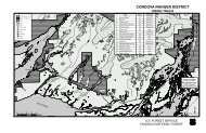
marten detections were not equally distributed across the LTB (Figure 1). Survey effort
was generally greater on the west and southeast portions of the LTB and relatively sparse
elsewhere (Figure 1). Detections in the northern and eastern portions of the LTB were
6

scarce, with martens only being detected at 1 sample unit to the east and 8 to the north
despite 30% of the total survey effort occurring in these two regions (Table 2). Martens
were most frequently detected on the western (50% of sites) and southern (31% of sites)
portions of the LTB.
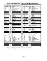
Table 1. Summary of survey effort for American martens in the Lake Tahoe Basin,
1993-2007.
________________________________________________________________________
Survey Year # Sample Units # Marten Detections
________________________________________________________________________
Project Surveys* 1993-2000 238 79 (33%)
East Shore 2005 48 2 (4%)
MSIM** 2002 22 9 (41%)
Marten-OHV 2003-04 43 36 (75%)
MSIM* 2002, 2005 58 31 (53%)
Urban Biodiversity 2003-04 77 17 (22%)
________________________________________________________________________
Total 1993-2007 486 174 (36%)
________________________________________________________________________
*Project surveys are surveys done prior to a management action (e.g., thinning)
**MSIM = Multiple Species Inventory and Monitoring study, piloted in the LTB. These
include Vertebrate Assemblage-OHV study locations as well.
Table 2. Survey effort and detections of martens by sub regions within the LTB. Survey
locations and detections represent unique locations. See Figure 1 for sub region
boundaries.
_________________________________________________________
Marten detections Number survey locations
Subunit (% of locations) (% of total effort)
_________________________________________________________
North 8 (9.6%) 83 (16.3%)
East 1 (1.5%) 67 (13.1%)
South 36 (31.6%) 114 (22.4%)
West 121 (50.1%) 244 (48.0%)
_________________________________________________________
TOTAL 166 (32.7%) 508
_________________________________________________________
7

The collection of surveys conducted during the last 15 years suggests that martens
appear to be well distributed on the west and south sides of Lake Tahoe, but are scarce to
the north and especially to the east of the Lake. The reduction in detections to the north
and east of Lake Tahoe are not surprising as these areas are more xeric than the west and
south, supporting forest habitats with lower suitability, due to their structure (e.g., more
open canopies, fewer large dead woody structures) and composition (e.g., pine
dominated), for martens. Campbell’s (2007) probability of occurrence model further
supports this trend in declining suitability to the north and east of the LTB (Figure 2)
based on habitat characteristics. However, there are two notable locations where
detection results shift noticeably and habitat suitability does not. The Highway 89
corridor west of Tahoe City and highway 207 (Kingsbury grade) corridor east of Tahoe
Village mark distinct transitions in the proportions of sample units with and without
detections (Figure 2). These highways and their associated urban development likely
represent filters for marten movement and will likely influence the persistence of the
martens to the north and east of Lake Tahoe. While the northern subpopulation likely is
connected with martens to the north of the LTB, the eastern subpopulation is likely
reliant entirely on the southern population for new recruits from dispersal.
Due to the lack of detailed historical information on the distribution of martens in the
LTB, we cannot compare the historical information to contemporary to evaluate the
contemporary status of the marten population in the LTB. We are left only with
contemporary distribution and known habitat relationships for the American marten to
define a reference condition. This said, the overall distribution of martens in the LTB is
likely similar to what is was historically, especially in the west and south regions of the
LTB. Distributional changes, specifically reductions in distribution, are expected in and
around the dense residential areas riming the lake as well as some reduction due to the
likely isolation of the small population remaining on the east shore of Lake Tahoe.
Declining number of detections in the northern and eastern regions of the LTB are
expected due to the shifts in the composition and structure of forest habitats from fairly
mesic on the west and south to more xeric in the north and east. However, it is likely that
anthropogenic effects (e.g., urbanization and highways that fragment these
subpopulations) may have contributed to further lowering the potential for these areas to
support marten subpopulations. At this time there is no information suitable for
evaluating whether a positive or negative trend in the marten population has or is
occurring. Thus, we will establish the current distribution reported here as the reference
condition from which the monitoring program will be built upon.
Bioregional Significance of the Lake Tahoe Basin Marten Population
The west shore population represents the only known contiguous linkage for marten
populations to the north and south of the Lake Tahoe Basin. Systematic surveys to the
west of the LTB and at lower elevations in Placer and El Dorado counties only detected
martens at 2 (4%) of 49 sample units (Zielinski et al. 2005). While portions of the
Desolation and Granite chief wilderness areas may still harbor martens in some areas that
were unsampled, these areas are dominated by large open expanses of granite and highly
8

fragmented patches of forest, unlikely to support martens or promote population
connectivity via dispersal. Maintenance of a well-distributed population of martens along
the west side of the Lake Tahoe Basin will not only benefit both local conservation of the
species, but could be critical for maintaining population and genetic connectivity for
martens in the north and central Sierra Nevada.
Development of the Conceptual Model
Monitoring of individual species is done to determine if management actions are
having the desired effects on these species. In the LTB, the management objective is to
maintain a self-sustaining marten population in the region. Because our review of the
historical and contemporary information on the distribution of martens leads to the
conclusion that martens are still well distributed in the LTB, the emphasis of the
monitoring program is on maintaining the marten population throughout its
contemporary distribution (reference condition; Figure 1). To ascertain compliance
with this management goal will require the initiation of a monitoring program capable of
detecting biologically meaningful levels of change in the marten population. If the
monitoring program demonstrates a lack of significant change in the marten population, it
supports compliance with the management goal. If the monitoring program demonstrates
a significant negative change in the marten population, it should trigger specific changes
in management practices.
The task of identifying a meaningful change requires some understanding of the levels
of change caused by natural intrinsic factors (e.g., severe winters) versus human-caused
extrinsic factors (e.g., timber harvest). Both can have population effects, but typically
species have had the time to evolve and cope with the natural variation in intrinsic factors
while they are not necessarily able to incorporate the additive variation from humancaused
extrinsic factors. Not all extrinsic factors may be detrimental to marten
populations, those that are, or hypothesized to, are hereafter referred to as stressors.
Stressor effects are evaluated in the context of induced changes to one or more
indicators (Noon 2003). Not all stressors are known nor are their relative magnitudes of
effects understood a priori. In the case of monitoring marten populations in the LTB,
there are a number of potential stressors that affect different portions of the LTB to
different degrees. Thus, stressor affects may be working independently in one area or
synergistically in another, and potentially in both spatial and temporal scales. All
monitoring programs need to acknowledge the complexities while attempting to tease out
important stressor effects. However, to embark on a monitoring program that does not
include the opportunity to learn about potential stressor effects, through challenging
multiple hypothesis about stressor effects with indicator data, misses an important
opportunity. The consequence of missing this opportunity would be embracing a
monitoring program to detect change, but with no way to indicate what is causing the
change.
A monitoring program can be designed to seek indicator-stressor relationships by
being retrospective or prospective. Retrospective monitoring or effects-oriented
9

monitoring seeks to find stressor effects after they have occurred by detecting changes in
the condition of a species’ population (NRC 1995). In contrast, prospective or stressoriented
monitoring attempts to detect the known or suspected cause of an undesirable
population effect, before the effect has a chance to become serious (Figure 3). Thus,
prospective monitoring, unlike retrospective monitoring, assumes prior knowledge of
cause-effect relationships between stressors and indicators (Thornton et al 1994).
However, cause-effect relationships for wildlife populations are seldom known with
certainty and are usually only suspected. In this case, a hybrid approach is necessary that
emphasizes simultaneous indicator and stressor measurement, and modeling the
relationships between stressor action, change in state of indicator, and subsequent
population effects (Noon 2003).
The hybrid approach is the best design for a monitoring program for American
martens in the LTB and is the approach used for effectiveness monitoring of the
Northwest Forest Plan (USDA et al. 1993). The first step in the design process for this
approach is to develop a list of the hypothesized stressors to marten populations in the
LTB. In section V (Identification of Stressors & Selection of Indicators) we will review
the existing information on stressors for martens and develop a list relevant to the LTB.
A conceptual model then identifies the scale-specific linkages between stressors and the
hypothesized population effects. Indicators that are indicative and predictive of the
anticipated changes in population condition are then selected for measurement (NRC
1995, 2000, Noon 2003).
Adding further complexity to the interpretation of monitoring results is that when a
monitoring program is initiated it begins with the effects of past stressors (e.g., logging
and ski resort development) and over the course of additional monitoring seasons
incorporates the combined effects of these past and additional future stressors (e.g., fuels
treatments; Figure 4). Thus the initial monitoring period provides an opportunity to
retrospectively evaluate past management effects by testing hypotheses representing their
suspected effects on population indicators. The knowledge gained from this retrospective
analysis can be used to better develop stressor-indicator relationships that can be
validated with future monitoring data (Figure 5). Thus, the value of using the initial
monitoring period to learn from past management, through retrospective analysis, should
not be underestimated and this learning opportunity not missed. In section VII, Data
Collection and Analysis, we will describe such an approach to implement after the first
data collection season.
Identification of Stressors and Selection of Indicators of Population Status and Change
A stressor is a factor that adversely affects individuals, populations, habitat, and/or
prey. While stressors can include those from both anthropogenic (extrinsic) and nonanthropogenic
(intrinsic) sources, we focus only on extrinsic stressors, those from
anthropogenic sources. Extrinsic stressors are the results of human action and therefore
can be altered if necessary through changing of management practices. There are a
number of stressors in the LTB that may have had historical and/or contemporary
10

negative effects on marten populations. Historical stressors may have caused declines or
local extirpations which may or may not have had time to be reversed since these
activities ceased. Historical stressors to American martens in the LTB include trapping,
predator & rodent poisoning, logging, and development (Lindstrom et al. 2000).
Potential contemporary stressors include some aspects of vegetation management,
continued urbanization, increased traffic volumes and speeds on roads, and the
development of and recreation related activities at ski resorts. The current status and
condition of the marten population will be a product of any lingering effects of past
stressors (e.g., areas still not recolonized due to the lack of regeneration of suitable
numbers of large live and dead woody structures removed by logging) and its current
responses to contemporary stressors. There have been recent reviews of the potential
effects that anthropogenic and non-anthropogenic stressors may have on martens in the
Sierra Nevada and we do not seek to repeat these efforts here (see USDA 2001, Green in
prep). We will provide a brief discussion of the 5 stressors we hypothesize to be the most
detrimental to the marten population in the LTB.
Urbanization
Urbanization has a number of known and potential effects on martens. The
conversion of forest habitat to urban uses (e.g., roads, houses) is a direct loss of habitat
and the fragmentation of remnant habitat in the vicinity. L. Campbell (pers. comm.)
found that marten occupancy in the LTB was significantly influenced by the distance to
urbanization and the patch size of habitat in the vicinity of urbanization. Indirect effects
are the high densities of predators and competitors (e.g., black bears and coyotes)
supported by food subsidies (e.g., garbage and other sources) that can increase mortality
of martens and reduce natural food resources in the vicinity of urbanization. Finally, the
high density of pets, specifically dogs, in urban areas can increase aggressive and
potentially fatal encounters for martens and facilitate both natural and non-native disease
transmission into the marten population and the animals martens come into contact with.
Ski Area Development & Operation
There are approximately 25 ski resorts in the Sierra Nevada mountains, nearly all of
which occur within the range of the American marten. The Lake Tahoe region includes
about half of these resorts, constituting the highest density of resorts in the Sierra Nevada
and one of the highest in North America. The development of ski resorts involves the
loss and fragmentation of forest habitat thru the removal of trees for creating ski runs,
creation of roads, and building of infrastructure (e.g., lifts, buildings). The operation of
ski resorts includes the continued compaction of snow, presence of high densities of
skiers, and nocturnal grooming activities. All these factors can have negative effects on
martens both directly (e.g., females may avoid these areas due to too much disturbance)
and indirectly (e.g., snow compaction and forest fragmentation facilitating higher
predation rates by coyotes and great horned owls, respectively). While martens have
been detected on many ski areas, Kucera (2004) found that the martens present on the
Mammoth ski area were nearly all males and only occupied the ski area seasonally.
11

Roads
Roads can affect martens by: 1) vehicle collision mortality 2) fragmentation of habitat
and population connectivity by acting as buffers, filters, or barriers to marten movement
and habitat use; and 3) indirectly by facilitating access by humans and predators (e.g.,
coyotes following snow compacted routes in winter) that results in mortality or avoidance
of the area. Robitalle and Aubry (2000) found that although martens can be detected near
roads, they tended to concentrate their activity away from roads. Not all road types have
the same effects. Paved roads with high-speed and frequent vehicle traffic likely
represent the largest threat for collision mortality and likely contribute the most to the
fragmentation of habitat and population connectivity. Secondary dirt roads are likely
most used by predators and may indirectly contribute to increased mortality of martens.
Vegetation Management
We use vegetation management here to define any management activity (e.g., timber
harvest, hazard tree removal, fuels treatment) that alters marten habitat. Vegetation
management can have both positive and negative effects, which can either have short or
long-term temporal impacts. A short-term negative effect of vegetation management is
the removal of overhead cover and escape cover, resulting is increased predation rates or
avoidance of the site. Canopy cover and some types of escape cover (e.g., dense shrub of
small diameter tree boles) can regenerate relatively quickly (e.g., 1-2 decades).
Vegetation management can also affect prey. Bull and Blunton (1999) found that fuels
treatments in lodgepole pine (Pinus contorta) and mixed conifer stands in northeastern
Oregon reduced key prey species (snowshoe hair [Lepus americanus] and red-backed
vole [Clethrionomys gapperi]) in treated stands. A critical long-term negative effect is the
removal of large-diameter live and dead woody structures, which provide resting and
denning locations, and take centuries to regenerate.
Motorized Recreation
Motorized recreation, which includes off-highway vehicles (OHVs; 4x4s, quads, dirt
bikes) and on-snow vehicles (OSVs; snowmobiles) have been considered potential
stressors due to the noise, speed, and locations where they can travel. However, Zielinski
et al. (2007) found no effects of motorized recreation on marten occupancy or activity
patterns of martens at the OHV/OSV use levels they observed in two study areas
(including the LTB) in the Sierra Nevada. In peak seasons of OHV/OSV use, martens
were naturally active in nocturnal and crepuscular periods of the day while OHV/OSV
users were largely diurnal, reducing the potential for encounters. Unless OHV/OSV use
increases above the levels observed in this study or OHV/OSV users become more
nocturnal/crepuscular in their recreational patterns, motorized recreation will likely
remain a non- or minor stressor for martens.
Linking Stressors to Marten Population Effects
12

The selection of indicators that reflect a species response to the underlying ecological
structural and functional changes resulting from extrinsic stressors requires a welldeveloped
conceptual model of the ecological system being managed (Manley et al.
2000). The foundation of this cause and effect conceptual model is found in Figure 3.
The ideal case would be to build a conceptual model from a foundation of knowledge,
based on rigorous investigation on how a species responds to individual stressors of
interest. In practice, this type of information is either lacking entirely or only available
from other geographic portions of a species’ range. This latter situation is where our
understanding currently stands on how American marten populations respond to
environmental changes. Using existing information and hypothesized relationships we
developed a conceptual model to link the 5 extrinsic stressors to likely responses by the
marten population in the LTB. The first step, was to identify the specific ways in which
each stressor affects relevant ecosystem functions. The second step was to link these
specific stresses to their ecological consequence, how they result in direct or indirect
changes to the system. The third step was to link these stressor induced ecological
consequences to marten population responses. It should be clear that this conceptual
model (Figure 5) represents a working hypothesis on how stressors affect marten
populations in the LTB. The resulting marten population responses are listed in relative
order of severity (Figure 5). These responses are related, such that as lower severity
effects are felt by a larger proportion of the marten population, they will begin to cause
more severe effects (e.g., reduction in distribution and decreased population viability).
The strengths of the linkages and the magnitude of their effects will depend on their
spatial extent (e.g., how much area is affected), intensity (e.g., degree of stressor effect),
temporal attributes (e.g., rate of stress), and synergistic effects when other stressors are
also present.
Table 7. Hypothesis about stressor effects on American marten occupancy patterns in the
Lake Tahoe Basin.
Stressors Hypothesized Effects
________________________________________________________________________
Urbanization, 1. Reduced Distribution: Negatively effects occupancy,
Ski Resorts, resulting in absence beyond a certain spatial threshold.
Vegetation 2. Reduced Female Occupancy: Females are more sensitive to
Management, males and avoid areas at lower development thresholds than
Major Roads males.
3. Increased rates of individual turnover (due to reduced
survivorship) at sites with the highest levels of urbanization.
4. Reduced detection probability due to lower use of habitat near
sites with stressor effects.
________________________________________________________________________
13

Indicator Selection
In the development of monitoring plans, selection of indicator(s) that directly relate to
the monitoring objective are required to provide the most useful inferences. As
mentioned in the beginning of this document, the management objective is to maintain
the marten population within its contemporary range in the LTB. Following the
management objective, the monitoring objective is to monitor the status and trend in the
marten population throughout its contemporary distribution in the LTB (Figure 1).
On the basis of the conceptual model and consideration of the management objectives
for martens in the LTB, we identify the following candidate indicators : (1) distribution,
(2) population size, (3) sex-specific occupancy, and (4) population turnover.
Survivorship, reproduction, and population viability assessment are more difficult and
costly to estimate and do not readily fit into a monitoring framework. For a general
review of Martes indicators, see Appendix 2.
Primary Indicators
One of the most detrimental population responses to one or more stressors is reduction
in geographic range. This can occur either through mortality or through permanent
movement away from an area that is no longer suitable. To estimate current geographic
distribution in the LTB, we will use site occupancy as an indicator.
Equally as important as site occupancy by martens is occupancy by females. Females
raise young on their own and need to maintain home ranges with suitable resources (e.g.,
den sites, prey populations) to enable them to reproduce and raise young until they
disperse. Several studies suggest that females may be more sensitive to certain stressors
(e.g., ski areas: Kucera 2004) than males. Furthermore females are on average 33%
smaller than males and may be more susceptible to mortality from stressors that involve
increased encounters with potential predators (e.g., reduction in overhead and escape
cover). Occupancy by females provides a more specific indicator of population status
than overall occupancy because it estimates the proportion of the LTB that is potentially
suitable for reproduction.
Occupancy by martens and occupancy by females both provide distributional
information but do not provide information on demographics. However, by using
ancillary data collected during the occupancy survey, e.g., gender differentiation of tracks
and collection of hair for DNA analysis, we will be able to make general inferences about
sex ratios and population size (see Secondary Indicators below).
A one-year estimate of occupancy rates by martens and occupancy rates by females
will enable us to estimate the proportion of the LTB that is likely occupied by martens in
general and females in particular. Comparison of occupancy rates between two or more
time periods will allow for estimating a trend in occupancy rate and to estimate whether
an overall decline has occurred. Investigation of the specific locations where changes
14

have occurred will allow for identification of where the declines are actually occurring.
Furthermore, patterns of occupancy can be specifically compared to the pattern and
intensity of both individual and multiple stressors (e.g., ski areas; see Evaluating Stressor
Related Effects). The initial sampling period offers both an opportunity to assess current
occupancy rates and –to the extent stressors can be quantified--how stressors influence
the occupancy rate. Subsequent sampling periods will primarily provide direct
comparison of both overall and site-specific occupancy status and secondarily will be
able to provide insight into how occupancy changes relative to changes in the magnitude
of stressor intensity (e.g., 2-fold increase in traffic volume on a highway) or spatial extent
(e.g., expansion of a ski area) where they occur.
Secondary Indicators
The secondary indicators are population size and population turnover and are included
to provide additional tools to investigate specific hypotheses about the primary indicators
and stressor effects. Secondary indicators require individual identification from DNA in
hair samples. By collecting hair samples concurrently with tracks, a number of genetic
methods are available to address additional questions. Of concern to LTB managers, as
well as anyone interested in using a related index to monitor a Martes population, is the
relationship between the index proposed here and the true population size. Hair samples
can be analyzed using existing genetic markers for martens for DNA fingerprinting to
address this concern. DNA analysis can determine how many individuals are present and
generate a population estimate. Once individuals are identified, the same sample units
can be resampled to make comparisons of turnover rates for individuals between sample
units with high and low exposure to stressors. Importantly, these secondary indicators
(population size and individual turnover rates) can only be used if hair samples are
collected and if additional funds are acquired to support their analysis.
Identification of Biologically Significant Indicator Thresholds
We propose a monitoring program capable of detecting a 20% decline in occupancy
rates by martens. Occupancy rates by female martens are unknown, but will be lower
than occupancy for both genders and may be insufficient for detecting changes in
occupancy rates over time. Given this unknown, the program will be designed around
occupancy rates for all martens, but will attempt to detect changes in and investigate
stressor relationships to occupancy by females. Because declines can progress slowly
(e.g., a small annual decline) or rapidly, we will provide a design and analytical tools
capable of detecting both types of declines. A slow decline requires the determination of
the trend of a population over a significant period of time and requires more effort to
detect than a rapid decline. A constant 2.2% annual rate of decline results in a 20%
decline over a 10-year period. Detecting this level of change over a shorter time period
(e.g., say over 3 years) requires less effort. A 20% decline represents a level of change
that is significant to a population and that we assume excludes natural fluctuations that
may occur due to annual variation (e.g., effect of winter severity on survival). This
threshold also matches the minimum standards for the National Inventory and Monitoring
15

Framework (April 3, 2000, http://www.fs.fed.us/emc/rig/iim) and matches the design for
monitoring the southern Sierra fisher population (Zielinski and Mori 2003, Truex 2003).
VI. Monitoring Approach Rationale
Section Objective:
Develop an analytical framework (e.g., sampling frame) appropriate for long-term
monitoring of the status and trend of the marten population in the LTB. For a general
review of marten monitoring methods, see Appendix 3.
Sampling Design
Our approach begins by saturating the LTB with a grid of hexagonal sample units,
each with an area of sufficient size to assume independence between adjacent sampling
units. We evaluated hexagonal sample units with areas of 2.5 km 2 , that have an area of
406 hectares, which exceeds the mean male (388 ha) and female (324 ha; Simon 1980,
Spencer 1981) home range sizes. We also evaluated hexagonal sample units with 3.0
km 2 , that have an area of 585 hectares, which exceeds the maximum home range sizes
estimated for male (537 ha) and female (526 ha) martens in the northern Sierra (Simon
1980, Spencer 1981). The distance between the center points of the 2.5 and 3.0 km 2
hexes is 2.16 and 2.59 km, respectively, and therefore, the 3.0 km hex size is more likely
to ensure independence between adjacent sample units. One hundred and forty-one 3.0
km 2 hexes occur in the LTB with the characteristics to support martens (Table 3, Figure
6).
Table 3. Potential Sample Unit hex statistics for the LTB. We used the predicted
probability of marten occurrence from Campbell 2007 to identify hexes with a high
(>50%) proportion of habitat with high predicted probability (>50%) of occupancy in
each hex.
Hex Diameter (km) Area OF Each Hex (ha) # of Hexes # of Hexes
in LTBMU in Habitat
____________________________________________________________________
2.5 406 260 ----
3.0 585 183 141
____________________________________________________________________
Sampling Method
The primary detection method is track plates (Zielinski and Kucera 1995). Track
plates provide an unambiguous and inexpensive method for distinguishing the tracks of
16

martens from other similar species (Zielinski and Truex 1998). To determine the sex of
martens present at each sample unit, we propose to use the track measurement methods
described by Slauson et al. (2008). To collect hair samples and provide information for
the secondary indicators, each track plate will also include a hair snaring modification,
such that hair samples suitable for genetic analysis can be collected concurrently with
tracks (see Design of Hair Snare Modification, Appendix 2).
Sample Unit Survey Protocol
Procedure: Each sample unit will be comprised of 3 track plate stations, 0.5 km apart, in
a triangle pattern (Figure 7). Sampling will occur from 1 June thru 15 August.
Rationale: To determine a survey duration with a high probability of detecting martens
present in the sample unit, we re-analyzed track plate data collected by Zielinski et al.
(2007). The data selected for this analysis were collected on the west side of the LTB in
2003, during the same season (summer, June-Aug) and using the same number of stations
per sample unit as we are proposing here. The station spacing used by Zielinski et al.
(2007) was half the distance (250 m between stations) that we propose here.
We used program PRESENCE (Version 2.0, Hines 2006) to fit models to the pooled
sex and sex specific detection history (e.g., 0011, 0101) data and estimate the parameters
of interest (e.g., p = probability of detection). We evaluated 5 models for each dataset
and determined that the 1-group with survey-specific probabilities of detection (SSP)
model performed the best across all datasets (Table 4). We used the parameter estimates
from the 1-group, SSP model to calculate the cumulative detection probabilities for each
dataset (pooled sex, male, female) (Figure 8). Using these estimates, a 12-day survey
duration, with visits every 3 days, yielded detection probabilities >95% for both sexes
combined, males, and females (Figure 8). Thus a 12-day, 4-visit sample unit survey
protocol should be adequate to ensure an adequate level of detection certainty for this
monitoring protocol.
Statistical Considerations
Background
It is essential to determine, a priori, the probability of detecting significant declines
and to choose an adequate sample size to be able to detect those changes with an
acceptably high probability. The null hypothesis, that there has been no change in the
population index over a 10-year period must be tested against the alternative that the
population has changed (either increased or decreased: two-tailed test) or declined (onetailed
test). Because the monitoring program is focused on maintaining martens
throughout their contemporary distribution in the LTB, we are only concerned with
detecting a decline (one-tailed test).
17

Table 4. Model results for pooled sex and sex specific detection history data from track
plate stations collected by Zielinski et al. (2007) during the summer of 2003 in the Lake
Tahoe Basin. w is the Akaike weight, which is considered the weight of evidence in
favor of a model being the best approximating model given the model set. K represents
the number of parameters in a model.
Data Set Model Model Name ∆AICc w K
Rank
________________________________________________________________________
Both Sexes
Male
Female
1 2 Group, SSP 0 0.55 10
2 1 Group, SSP 0.61 0.41 5
3 3 Group, SSP 5.68 0.03 15
4 2 Group, CP 10.31 0.00 4
5 1 Group, CP 12.46 0.00 2
1 1 Group, SSP 0 0.90 5
2 2 Group, SSP 5.00 0.07 10
3 1 Group, CP 7.34 0.02 2
4 2 Group, CP 10.31 0.00 4
5 3 Group, SSP 11.44 0.00 15
1 1 Group, SSP 0 0.86 5
2 1 Group, CP 4.40 0.10 2
3 2 Group, SSP 6.90 0.03 10
4 2 Group, CP 8.41 0.01 4
5 3 Group, SSP 11.42 0.00 15
________________________________________________________________________
SSP = Survey-specific probability of detection, CP = Constant probability of detection.
Statistical Power Simulations
We calculated statistical power using two programs written by J. Baldwin (PSW
Statistician) using SAS (v8, SAS Institute 1999) that samples simulated datasets created
using parameter estimates from field data. For field data we used the same data from
Zielinski et al. (2007) used in the previous section (see Sample Unit Survey Protocol).
We simulated a decline, set at 20%, in the population index over a 10-year period. We
selected a one-tailed test because we are only interested in determining whether the index
has declined from one sampling period to the next. Selecting a one-sided test has more
power than a two tailed test at the same α level, and thus requires a smaller number of
sample units (approximately 50% fewer) and a smaller budget.
18

For the 10-year trend power analysis, we first had to determine the optimal sampling
frequency within the 10-year period. To determine this, we conducted prospective power
analyses varying the number of years in which surveys are conducted while holding all
other values constant (Table 5). The number of surveys has a small effect on power.
However, the most optimal design is for 4 surveys conducted at 3-year intervals and this
design will be used for the next phase of the power analysis.
Table 5. The effect of the number of surveys and the survey interval on power. α, ψ, and
the number of sample units were set at arbitrary levels and held constant.
α Power Initial Occupancy Sample Units # Surveys Years
(ψ) (interval) Sampled
________________________________________________________________________
0.2 0.81 0.7 90 2 (5) 1,10
0.2 0.76 0.7 90 3 (4) 1,5,9
0.2 0.84 0.7 90 4 (3) 1,4,7,10
0.2 0.81 0.7 90 5 (2) 1,3,5,7,9
________________________________________________________________________
A prospective power analysis is only useful when realistic values are used for the
parameters required to conduct it. In an occupancy modeling power analysis, the initial
proportion of sample units occupied (ψ) has a strong influence on the sample size that
will be required to detect a decline in the index. To determine a likely range of initial
proportions of sample units occupied by martens, we extrapolated from the contemporary
surveys effort conducted across the LTB.
Using data from Zielinski et al. 2007, we first determined which of the 183 sample
units (3.0 km 2 ) had survey effort (126, 67.7%) and of those how many had marten
detections (64, 50.7%). This represents a simplistic lower estimate of the proportion of
sample units likely to be occupied. However, because suitable habitat for martens is not
uniformly distributed across the LTB, it would be unreasonable to assume that martens
would occupy all sample units across the LTB. To remove sites with no or very little
suitable habitat we used Campbell’s (2007) predicted probability of occurrence coverage
to identify sample units that have >50% of the area (>292 ha) of habitat with >50%
predicted probability of occurrence. Forty-two (22.9%) of the sample units did not meet
these criteria and 141 (76.0%) did. Surveys had been conducted at 25 (59.5%) of the 42
sample units not meeting the suitability criteria and 101 (71.6%) of 141 sample units
meeting the suitability criteria. Martens were only detected at 4 (16.0%) of the 25 sample
units not meeting the suitability criteria, while they were detected at 60 (59.4%) of the
101 sample units surveyed that met the suitability criteria. We used the proportion of
sample units meeting the suitability criteria ~60%, as a more realistic estimate of initial
occupancy, and also varied this by ±10% (Table 5). We also included an initial ψ of 0.8
to show how the sample size can be reduced if initial occupancy is higher than we have
estimated.
19

Next, we parameterized the simulation with detection probabilities estimated from
field data. We set the number of visits to each sample unit at 4 for each simulation and
used the individual visit detection probabilities (p1= 0.43, p2 = 0.43, p3 = 0.61, p4 = 0.86)
generated from track plate data collected during the summer in the LTB using the
protocol proposed here (see Zielinski et al. 2007). A markov persistence factor was set at
0.5 to account for the dependence in detection outcomes between visits (Slauson et al.
2008b).
The most realistic estimate of occupancy in the initial sampling period is 0.6, however
an occupancy rate of 0.7 would not be unexpected if sample units are selected above
some minimal suitability value. Using an occupancy rate of 0.6 and an alpha of 0.15 or
0.20, would require 110 and 140 sample units to detect a 20% decline, respectively
(Table 6a). Using an occupancy rate of 0.7 and an alpha of 0.15 or 0.20, would require
80 and 100 sample units to detect a 20% decline, respectively (Table 6a). Based on these
statistical considerations, we recommend a sample size of 110 (Table 6a) be randomly
selected from the 141 sample units with the minimal suitability criteria. If the initial
proportion of sample units occupied from the first year of sampling is ≥0.7, then the
sample size could be reduced if desired.
Table 6. Prospective power analysis results for (A) detecting a 20% decline in the marten
population index for an entire 10-year period (sampled every 3 years) when there are 4
survey periods and (B) the level of change capable of being detected between any two 2
time periods during the 10-year period, under the varying parameter conditions listed.
A. Trend Over 10-years (4 sampling occasions)
α Power Initial Occupancy Sample Units
(ψ) Required
_______________________________________________________________
0.10 0.80 0.5 250
0.10 0.80 0.6 175
0.10 0.80 0.7 120
0.10 0.80 0.8 80
0.15 0.80 0.5 200
0.15 0.80 0.6 140
0.15 0.80 0.7 100
0.15 0.80 0.8 65
0.20 0.80 0.5 160
0.20 0.80 0.6 110
0.20 0.80 0.7 80
0.20 0.80 0.8 50
_______________________________________________________________
20

B. Detectable Level of Change Per Sampling Interval (3 Years)
α Power Initial Occupancy Sample Detectable
(95% C.I.) (psi) Units Decline
_______________________________________________________________
0.15 0.83 0.5 110 20%
0.15 0.81 0.6 110 17%
0.15 0.81 0.7 110 15%
0.20 0.82 0.5 110 18%
0.20 0.81 0.6 110 15%
0.20 0.82 0.7 110 12%
_______________________________________________________________
While we have developed the monitoring program to detect a trend over a 10-year
period, declines may occur more rapidly. To address this potential we conducted a
second power analysis to determine what level of change could be detected between any
two sampling periods (3 year interval) given there will be 110 sample units included in
the monitoring program. With a sample size of 110, a 12% to >20% to be detected
between any two time periods during the 10-year sampling period. Thus, the program is
capable of detecting both slow and rapid rates of decline.
Evaluating Stressor Related Effects
Stressors will be treated as site specific covariates and used to explain the patterns of
marten occupancy. Models consisting of single stressors and combinations of >1 stressor
will be compared to a model without stressor affects (null model). It is important to
understand that this analysis will only produce marten-stressor associations, and while
they can suggest cause and effect relationships, focused research efforts will be necessary
to confirm these relationships. However, the detection of marten-stressor associations, if
present, is an important step toward developing management strategies to protect the
marten population in the LTB.
We previously identified the four primary stressors and linked them to their
hypothesized effects on martens (section III, Figure 5). These hypotheses can be
translated into competing models to describe patterns of species and sex-specific
occupancy.
The measurement of stressors must take into account the temporal and spatial extent
of the stressor as well as its intensity. In addition, each stressor must be measured in a
manner appropriate to match the resolution of the marten data being collected. To
achieve this match we propose that stressors be measured at the scale of the sample unit
and with regard to their spatial extent of influence in each sample unit. Thus for each
stressor, a GIS coverage will need to be created to identify the spatial locations of each
21

stressor. For each stressor, we identify important elements of temporal extent and
intensity to include in their measurement (Table 8). For example, vegetation
management has been conducted in several forms (e.g., selective logging, fuels
treatments) occurring over several decades and should be measured to maintain the
differences of method and time. Additional stressors can be added to this analytical
framework if new information warrants their inclusion.
Table 8. Stressor data layers to be used or created and be used as the basis for measuring
stressor influence for each sample unit.
Stressor Data Source
________________________________________________________________________
Urbanization Parks et al. (in review) Urbanization Index for the LTB
Ski Resort Create a coverage with the footprints of all ski resorts in the LTB
Vegetation Fuels Treatments- at this stage a single coverage to identify the
Management areas treated, when they were treated, and how they were treated
(e.g., treatment prescription)
Past Logging- assemble a coverage identifying the spatial extent,
date when it occurred, and the type (e.g., selective, clearcut) of
past logging in the LTB.
Major Roads Use existing coverages to create a single coverage including all the
major routes of travel for high-speed (e.g., >35mph) vehicles.
Assign each route a relative traffic volume category (e.g., high,
medium, low volume).
________________________________________________________________________
Cost Estimates for Field Data Collection
The final element required to evaluate the number of sample units to be included in
the monitoring plan is the cost to collect field data. To generate realistic estimates we
will first estimate the total number of hours required to complete a single sample unit.
Then this estimate can be multiplied by the total number of sample units and then by the
cost to government for field technician time.
Based on our experience deploying the same sample units in the LTB we estimate
that, on average, 3 sample units can be set up or checked in a single 10 hour work day.
Each sample unit will require 3.33 hours per visit. Each sample unit requires 5 visits, the
first to set it up, then 4 checks. Sample units are set up most efficiently with 2 field
technicians, while all subsequent visits can be done by a single technician, including the
final visit when the sample unit is pulled. Thus each sample unit will require 6 technician
22

visits, equaling (6 * 3.33) = 19.98, or ~ 20 total hours to complete. We used the estimate
of 20 hours per sample unit in the Table 9 to illustrate the costs for field data collection
for several alternative sample sizes.
Table 9. Estimated costs for field data collection for a single sampling period. All
estimates are for FY 2007 costs and do not include annual wage increases. A 25%
increase was added to each estimate to include training hours, leave, and unforeseen
additional costs. The gray highlighted row indicates the costs for the selected design.
Sampling Strategy
Number of Total Cost for Field Labor 1-Year 10 –Year
Sample Units (GS-5 2007 Cost to Govt.) Complete Program*
________________________________________________________________________
45 [(45 * 20) * $14.88]*1.25 = $16,740 $66,960
55 [(55 * 20) * $14.88]*1.25 = $20,460 $81,840
65 [(65 * 20) * $14.88]*1.25 = $24,180 $85,920
70 [(70 * 20) * $14.88]*1.25 = $26,040 $104,160
80 [(80 * 20) * $14.88]*1.25 = $29,760 $119,040
110 [(110 * 20) * $14.88]*1.25 = $40,920 $163,680
140 [(140 * 20) * $14.88]*1.25 = $52,080 $208,320
________________________________________________________________________
*This is for 4 sampling occasions, once every three years, for 10 years.
Equipment, Data Management, and Analysis Costs
The additional costs for the program include the initial equipment required to conduct
the work (Appendix 4) and the support staff time required to supervise field crews, enter
and proof data, conduct analysis and write up the results. These costs will depend on the
amount on new equipment needed. In general the cost per track plate station (coroplast,
aluminum plate, hardware cloth screen, etc) is approximately $20/station. To complete
110 sample units during the survey season (June 1 – August 15), 28 sample units will
need to be surveyed simultaneously every 2-week period; resulting in a minimum of 84
stations needed to comply with this schedule. Adding a few extra stations to serve as
back ups and for additional sample units during easy sample unit assignments, we
recommend the program have 110 stations on hand (110 * $20 = $2,200 for purchasing
station supplies). We generally estimate that it will take 2 months of time to confirm and
measure marten tracks, enter and proof database. Costs for the previously mentioned
duties will depend on whether staff time for existing employees will be dedicated for this
project or not. We strongly recommend that the individuals likely to conduct the first
23

year(s) of analysis consult with the principal investigators to ensure proper treatment of
the data, proper execution of the analysis, and to be able to incorporate any advances in
the types of analysis available for the data.
Sample Unit Selection
Now that we have determined the optimal number of sample units to include in the
monitoring program, the next step is to randomly select 110 sample units from the 183
available. The first step in this process is to remove any additional sample units that meet
the following criteria: (1) are composed of >80% urban areas (2) have no moderate-high
areas of predicted probability of occurrence using Campbell’s (2007) model (3) are
composed of >50% water (4) have

Table 10. General movement patterns of American martens and logistical (e.g.,
fieldwork and budget costs) relationships by season.
Season American Marten Movements Field Logistics
Juvenile Adult Male Adult Female & Costs
________________________________________________________________________
Fall (Sept-Nov.) High Low Low Low-High
Winter (Dec.-Feb.) Low Low Low High
Spring (Mar.-May) Moderate Low Low High-Moderate
Summer (Jun.-Jul.) Low Moderate? Low Low
________________________________________________________________________
VII. Data Collection and Analysis Protocol
Section Objective:
The objective of this section is to provide the details necessary to conduct field data
collection, analyze field data, and reach conclusions about the status of marten population
in the LTB using the monitoring approach detailed in the previous section.
Field Protocol
Establishing Sample Units
Prior to establishing any sample unit, the sample unit stations should either be plotted
on a 1:24,000 USGS topographic map or on a GIS generated map. If hand plotted, a
1:24,000 UTM grid will be necessary to locate the approximate locations for each station.
UTMs for stations in all selected sample units can be found in Appendix 5. When
necessary, stations can also be plotted on 1:10000 digital ortho quarter quads (DOQQs).
Plotting and studying stations locations and access options should allow for the selection
of the most safe and efficient access routes into sample units. Coordinates should be
programmed in to GPS units as waypoints while in the office, prior to installing the
sample unit. Field personnel will use a map, compass, and GPS to navigate within 20 m
of station locations.
Placement of Track Plate Stations
Once field personnel have identified the station location, a suitable site for setting the
track plate station must be selected. Ideally, track plate stations should be established on
level terrain so field personnel must create a level surface by digging or piling debris. A
level surface is critical for stability of the station, encouraging animals to enter the box,
and for the collection of high quality tracks. Track plate stations should be set against a
log, rock, tree, shrub or other ground feature. Stations should be further stabilized by
25

piling forest debris (e.g., logs, branches, rocks) on the sides and top of the box. However,
make sure not to pile heavy objects on top of the box as these may collapse the box.
After track plate boxes have been built and set up, each track plate should be prepared
and baited. Attach contact paper sheets to each track plate prior to leaving for the field
using the specifications in Appendix 2. Place track plates at the entrance of each station,
as flat as possible, prior to application of toner. Apply a thin layer of toner to the entire
entrance portion of the plate. Distribute the toner from a bottle uniformly on the plate
and then spread evenly using light dabbing vertical strokes with a make-up brush. After
toner is applied, remove the wax cover sheet from the contact paper (exposing the sticky
surface), place bait on the rear untonered portion of the plate, and gently slide the plate
into the box. Make sure the plate sits flush with the bottom of the box by tapping on the
front edge. Place small bits of duff (e.g., bark) under the non-flush edges of the plate
when necessary to stabilize it.
Application of Lure
Place a commercial trapping lure (GUSTO TM , Minnesota Trapline Products, Pennock,
MN, http://www.minntrapprod.com/) on an elevated location near each station. Ideally
lure will be applied to the bole of the tree nearest to the track plate station, at a height of
approximately 2m. GUSTO is best applied when mixed thoroughly with lanolin at a ratio
of roughly 3onces GUSTO/1 lb lanolin.
Monumenting Station Locations
Monument each station location to facilitate accurate resampling. We recommend
placing a numbered tree tag in the tree at the station location and 4 alternative tree tags in
trees at each of the 4 cardinal directions; each alternative tag is placed at breast height on
the tree, facing the station tree.
Station Relocation
Field personnel will create flaglines to connect stations to the access points in the most
efficient and safest routes of travel. Each station should be identified with two flags
labeled with the appropriate information (Sample unit #, Station, Date established) using
a Sharpie TM pen. Flag lines should be dense enough so that the next two flags can be seen
when traveling any direction along the route. Two flags will be placed at the point of
access (e.g., road or trail) for the sample unit and labeled with ‘Access to’ and the
appropriate sample unit number(s). Flagging must be removed when the sample unit is
removed. Alternatively, if GPS units are to be used, only flags in each of the 4 cardinal
directions, 10 m from the station and 2-flags at the actual station will be sufficient for
efficient relocation.
26

Revisits to Stations
Revisits to each sample unit occur every 3 days and the sample unit is removed on the
4 th visit (after 12 days). During each visit, gently remove the track plate out of the track
plate box and examine it for the presence of tracks. Tracks occurring on the soot or
contact paper should be collected. Tracks on toner should first be photographed with a
digital camera. First place a metric ruler parallel to the central axis of the best track(s) on
the toner. Then label a small piece of paper with the sample unit – station – date and
place it next to the rule and track. Then take photos that fill the frame with the track,
scale, and site/date label together. Archive digital photos of tracks in a database
immediately upon return from the field. Tracks on contact paper should be labeled (do
not write over carnivore tracks) with a sharpie (Sample unit #, station: 35-1, date: DD-
MMM-YY, observer’s 3 initials: KMS), removed from the track plate, and placed in an 8
1/2 x 11 inch acetate document protector. Store document protectors and tracks in a
tatum or similar device such that tracks are not folded or crushed. Small squares of
contact paper can be used to try and ‘lift’ tracks on toner only. This process is not always
successful and usually alters the tracks such that detailed measurement for sex
discrimination may not be possible. However, to do so remove the wax paper cover and
firmly place the sticky side on top of the track(s) of interest. While keeping the contact
paper completely stable (not sliding laterally), firmly rub the area of the track with your
thumb with as much pressure as is tolerable. If successful and a quality track is removed,
label it appropriately and place in a document protector. All station visit data is recorded
on the Daily Track Plate Form (see Appendix 5 for example) while at the station.
Collection of hair samples
After inspecting the track plate, remove the binder clips on the track plate box
and open the top of the box to inspect the hair snare. If marten tracks are present or
suspected, all hairs should be collected. Visually inspect the snare by removing it from
the box, if hairs are present, put the snare into the storage container with silica gel
indicator desiccant (Sorbead Orange, eCompressedair, Tulsa, OK) and label the container
the sample information as the contact paper section with tracks (see description above).
Bait
Add or replenish bait during every visit. Bait present from the last visit should be
removed (wrap it up in excess wax paper and store in sealable baggies) and disposed of in
a dumpster. Do not discard old bait in the field, especially near a sample unit!
Data Management and Analysis Protocol
The following section details the steps involved from after field data are collected to
data analysis. The process is a sequential and should follow the sequence presented in
Figure 10.
27

Field Data Forms, Tracks, and Hair Samples
Field data forms should be stored chronologically. Tracks should be stored by
sample unit. Hair samples should be grouped by sample unit and kept in a cool, dry, and
dark, airtight container.
Track Identification
All tracks must be reviewed in the office to confirm field identification of all marten
and other species tracks using the morphological and measurement details in Taylor and
Raphael (1988), Zielinski and Truex (1998), and track examples at:
http://www.fs.fed.us/psw/topics/wildlife/mammal/tracks.shtml).
Proof Daily Track Plate Forms
After confirming the identity of all tracks, review the Daily Track Plate forms to proof
the identification of the species listed on the forms. Be sure to check over all other fields
for completeness (e.g., all fields should contain data entries) and correctness. Sign and
date each form upon completion of proofing to track this process.
Sex Discrimination of Tracks
All confirmed marten tracks should be subjected to the evaluation and measurement
protocol described in Slauson et al. (submitted; Appendix 4). Two observers should
independently measure the tracks to ensure proper measurement and agreement of gender
identification.
Complete Station Summary Forms
The first step in collating field data is to complete a Station Summary Form (see
example in Appendix 4) for each station in every sample unit. These forms will combine
the data for all visits to each individual station. For each station to be summarized, the
Daily Track Plate forms with the data for each visit will be required.
Create a Database
Create a database format that will allow for the entry of data from station forms. The
database should be stable, allow for easy data entry, and for querying for data with output
formats suitable for use in statistical programs (e.g., SAS). Additionally, enter all marten
occurrences in NRIS Wildlife so that they are available to other Forest Service units.
Proofing the Database
Once all the data has been entered from the Station Summary Forms, the database will
need to be proofed to correct any entry errors. First create individual Station printouts for
all stations in the database and then compare the printout from the database with the
28

Station Summary Forms to confirm accuracy. Sign and date all forms once they have
been proofed. Update database with all corrections made. Once the database has been
completed, create a backup for the original field forms and database and store the
backups at a second location.
Data Analysis
Preparation of the Marten Analysis Dataset
Once the database has been completed and proofed, it can be queried to produce the
analysis datasets. Creation of the analysis datasets consists of creating a detection history
for martens by visit, across all stations within a sample unit. Each visit to a sample unit
will receive a ‘0’ if no martens were detected at any of the 3 stations or a ‘1’ if a marten
was detected at 1-3 off the stations. Survey visits missed should be marked with a ‘.’ or
equivalent missing data value for the statistical software being used. Thus, a sample unit
that detected martens on the 1 st and 3 rd visits would have a detection history of 1010.
Gender-specific detection histories will also need to be created for all sample units. For
each visit to a sample unit, a ‘0’ is entered when no females were detected, ‘1’ if 1-3
stations detected a female marten, and ‘.’ is entered if the track was not identifiable to
sex.
Occupancy Estimation, Status, & Trend Analysis
The first step in estimating occupancy is to fit a model to the detection history data.
This process follows the example provided in the Sample Unit Survey Protocol section,
using the same set of competing models and adding any new models hypothesized to
better fit the data. These models will be fit separately to each analysis dataset (e.g., all
martens, female only) and for each year of sampling (e.g., 2008, 2011).
The candidate set of models incorporate both standard models included in program
PRESENCE (version 2.0, Hines 2006) and custom models representing hypotheses on
how additional covariates may influence detection probability. Standard models included
covariates that assume p is constant across visits (constant p), that estimate p individually
for each visit (visit-specific p), and assume that heterogeneity exists in the data such that
the data are better modeled if partitioned into two groups (2-groups). Custom models
included variables found to be important in the analysis of fisher detection data at track
plate and remote camera stations in California (Slauson et al. 2008). Use the SAS
analysis procedure listed in Appendix 5 to conduct this analysis.
The relative performance of all models to describe the detection history data are
evaluated by comparing their AICc values and AICc weights (w) (Burnham and Anderson
2002). The top model(s) are used to estimate the probability of detection (p) and
occupancy (ψ). Estimates of occupancy (ψ) and their associated coefficients of variation
(e.g., SE’s) will be used for the status and trend analysis described next.
29

Status & Trend Analysis
The analysis of monitoring data taken from the same locations over >1 time periods is
done using the ‘multi-season’ trend analysis in program PRESENCE. However, when
only two time periods are being analyzed, the procedure simplifies to a paired t-test. For
the analysis of the full 10-year trend dataset, the analysis assumes a linear change over
time. Further explanation of the statistical procedures can be found in the help menu of
program PRESENCE and in MacKenzie et al. 2005.
Analysis of Stressor Effects
Stressor effects will be evaluated by including each stressor as a ‘site’ covariate in
program PRESENCE. Add the sample unit specific stressor attributes to the marten
analysis data set. Run the analysis with the competing model set for sample units with
stressor covariates. Relative performance of the models will be assessed using the AIC
diagnostics described above.
Use of Hair Snare Data for Specific Hypothesis Testing
The collection of hair samples allows for the testing of several additional hypotheses
that relate to assumptions of the sampling design, testing for stressor-related effects, and
investigating the role of density-detection probability relationships. The selection of
sample units for these additional efforts will depend on the results of the sample units
detecting martens. In general, sample units should be selected that have the best chance
to evaluate the hypotheses listed in table 10. These hypotheses are not exclusive and
samples from the same sample unit can be used to address more than one of these
hypotheses or additional hypotheses not listed. The sample units selected and types of
analyses planned should be done with consultation with the principal investigators or
other qualified analysts. At the current time, genetic analysis to determine the individual
identity of marten from hair samples costs ~$100/sample (M. Schwartz, USFS Carnivore
Genetics Laboratory, pers. comm.). Thus, analysis of hair samples should not be done
without careful consideration to maximize the use of analysis funds.
Quality Assurance and Quality Control
Ensuring Accurate Field Data Collection
Supervisors of field crews should make unannounced visits to sample units with field
personnel to evaluate the accuracy of execution of the sampling and data collection
protocol. Field supervisors should conduct routine screening of all data forms to ensure
completeness and accuracy. Field supervisors are responsible for correcting errors in
execution of a field related protocols.
30

Table 10. Hypotheses to address using individual marten identification data generated
from DNA fingerprinting using hair samples from hair snares.
Hypothesis How to Test
________________________________________________________________________
1. Sample units are independent, Select clusters of adjacent sample
adjacent sample units do not detect the units with marten detections.
same individuals. Analyze all hair samples and
determine whether any individual are
detected at more than 1 sample unit.
2. There is no difference between the number Select sample units with high and of
individuals detected in sample units with high low stressor exposure. Analyze all
versus low stressor exposure. hair samples and determine whether
the number of individuals present
differ.
3. There is no effect of the number of individual Determine the number of present
martens detected in a sample unit and detection across the gradient of detection
probability. histories.
________________________________________________________________________
Evaluation of Data Accuracy
We have previously provided mechanisms for supervisor review of field data,
verification of tracks, and proofing of data of field forms, and in the final database.
Evaluation of Analysis Accuracy
Both interim and final analysis should either be completed in collaboration with the
principal monitoring program authors or with others experienced in the analysis and
interpretation of the carnivore monitoring data. One or more independent reviews from
researchers well qualified to evaluate this type of analysis, the results, and their
interpretations is also suggested.
Equipment and Training
Field Data Collection
A detailed list of the required equipment is listed in Appendix 4. Individuals involved
in field data collection should be well trained in navigation with both GPS and mapcompass-altimeter
together top have the ability to accurately locate stations. Field
personnel should receive training on track identification sufficient to be able to reliably
distinguish marten tracks from all others anticipated to occur in the area. Field personnel
31

should be trained in data collection procedures involved. All field personnel should be
trained in first aid and in communication protocols (e.g. use of radios). Prior experience
in any or all of the above is preferential.
Track Identification and Measurement
Training for track identification should be conducted for all individuals involved in
field data collection. These individuals will be responsible for taking care to properly
identify, collect, and transfer original field data from track plate stations to the office.
They must be able to identify marten tracks or potential marten tracks from all other
species and have the ability to transfer tracks from soot to contact paper in the event of
soot-only tracks. Measurement and positive identification of tracks should be done
indoors and under well lighted conditions. Measurements should be done by as few
persons as possible to reduce individual variation and should be done with digital
calipers.
Training for track identification should involve reading of the following resources:
Taylor and Raphael 1988), Zielinski and Truex (1995), and Slauson et al. (submitted) as
well as studying on-line examples of tracks collected from known individuals at:
http://www.fs.fed.us/psw/topics/wildlife/mammal/tracks.shtml.
Track measurement for distinguishing sex should be conducted by as few individuals
as necessary to reduce observer variation. Ideally, only two individuals should measure
tracks independently. Results of measurements should be compared for consistency in
sex identification.
VIII. Flexibility in altering the monitoring program
The monitoring program has the capacity to be flexible to some changes. The most
significant consideration of alteration of the program should take place after the first year
of its implementation. After the first year, actual estimates of initial occupancy will be in
hand to determine the most optimal number of sample units to include. If the budget is
not available to complete the entire grid of sample units, a subset with a higher initial
occupancy level can be strategically selected to monitor, but this should be done
cautiously with full consideration of the affect on the program’s ability to detect the 10year
trend in change. Significant changes to the program should be done in consultation
with the authors or others well experienced with the monitoring and analytical methods
used in the program. Additional stressors can be added to the analysis if warranted.
IX. Applicability of this Protocol to other mesocarnivores in the LTB.
The LTB marten monitoring program is designed to be compatible with the national
monitoring framework for the Multiple Species Inventory and Monitoring (MSIM;
Manley et al. 2006) protocol. It represents a species specific extension. The detection
device selected in this protocol, the track plate, are capable of detecting mesocarnivores
as large as the fisher and gray fox (Urocyon cinereoargenteus; Zielinski et al. 2005). The
32

only large carnivore species reliably detected by track plates is the American black bear
(Ursus americana; Zielinski et al. 2005). However, bears do not always leave verifiable
tracks, despite visiting and disturbing stations. Two large-bodied mesocarnivores found
in the LTB, the coyote (Canis latrans) and bobcat (Felis rufus), are not reliably detected
using track plates (Campbell 2004). Other detection devices (e.g., cameras and open
track plates)
can result in somewhat higher frequencies of detection, but still would not yield a high
probability of detection of these species with similar survey durations as the 12-day
protocol proposed here (Campbell 2004). Coyotes can show both avoidance of detection
devices (Gompper et al. 2006) and attraction to them, both of which has been observed in
the LTB (Slauson pers. obs, Campbell pers. comm., respectively), confounding the
interpretation of detection results. There are no current field methods that could be added
to the proposed protocol to include a probability of detection of bobcats and coyotes. In
Table 11 we present the species of mesocarnivores potentially present in the LTB and
their likelihood, based on synthesis of relevant literature and our judgment, of being
detected adequately by the proposed track plate protocol.
Table 11. Species of mesocarnivores known to occur in or near the LTB and their
relative detectability using the proposed 3-station track plate protocol.
Species Relative Distribution Detectability with
in LTB Proposed Protocol
_____________________________________________________________________
American black bear Widespread High
Mountain lion Unknown Low
Bobcat Rare Low
Coyote Widespread Low
Gray fox Rare High
Marten Widespread High
Long-tailed Weasel* Unknown Moderate?
Short-tailed Weasel* Unknown Moderate?
Spotted Skunk Rare High
Striped Skunk Unknown/Urban Assoc. High
Raccoon Urban Associate Moderate?
Ringtail Unknown/Rare High
_______________________________________________________________________
*Weasels are not distinguishable based on track morphology.
Acknowledgements
We would like to thank Jan Werren for GIS support and Christina Voitja for reviewing
this document.
33

Literature Cited
Bryliski, P. V., P. W. Collins, E. D. Pierson, W. E. Rainey, and T. E. Kucera. 1997.
Mammalian species of special concern in California. Department of Fish and
Game, Sacramento, California, USA.
Bull, E.L., and A. K. Blumton. 1999. Effect of fuels reduction on American martens and
their prey. Research note, U.S.F.S., PNW-RN-539. 8 p.
Bull, E.L., and T. W. Heater. 2001. Survival, causes of mortality, and reproduction in the
American marten in northeastern Oregon. Northwestern Naturalist 82:1–6.
Burnham, K. P., and D. R. Anderson. 2002. Model selection and multi-model inference:
A practical information-theoretic approach. 2 nd Edition. Springer-Verlag, New
York.
Campbell, L. 2004. Distribution and Habitat Associations of Mammalian Carnivores
in the Central and Southern Sierra Nevada. Dissertation, University of California,
Davis. 167 p.
Campbell, L. 2007. Predicted probability of occurrence for American martens in the
Lake Tahoe Basin. Un published report. PSW, Sierra Nevada Sciences Center,
Davis, CA.
Cohen, J. 1988. Statistical power analysis for the behavioral sciences. Second edition.
Lawrence Erlbaum, Hillsdale, New Jersey, USA.
Field, S. A., A. J. Tyre, H. P. Possingham. 2005. Optimizing allocation of monitoring
effort under economic and observational constraints. Journal of Wildlife
Management 69(2):473-482.
Gompper, M.E., R.W. Kays, J.C. Ray, S.D. LaPoint, D.A. Bogan, and J.A. Cryan. 2006.
A comparison of noninvasive techniques to survey carnivore communities in
Northeastern North America. Wildlife Society Bulletin 34:1142-1151.
Green, G. A. In prep. California marten conservation assessment.
Grinnell, J., J. S. Dixon, and J.M. Linsdale. 1937. Fur-bearing mammals of California.
Vol. 1. University of California Press, Berkeley, CA.375 pp.
Hines, J. E. 2006. PRESENCE version 2.0. Software to estimate patch occupancy and
related parameters. USGS-PWRC.
http://www.mbr-pwrc.usgs.gov/software/presence.html
Kucera, T. 2004. Ecology of American martens on the Mammoth Ski area.
Unpublished report.
34

Lindström, S., P. Rucks and P. Wigand. 2000. A contextual overview of human land use
and environmental conditions. Pages 23 - 127 In: Murphy, D. D., and C. M.
Knopp, editors. Lake Tahoe Watershed Assessment: Volume I. USDA Forest
Service, General Technical Report PSW-GTR-175, Albany, California. 753 p.
MacFarlane 2007. Sensitive species list for Region 5. Unpublished report, Region 5,
Vallejo, California.
MacKenzie D.I., J.D. Nichols, J.A. Royle, K.H. Pollock, J.E. Hines, and L.L. Bailey.
2005. Occupancy estimation and modeling: inference methods for patterns and
dynamics of species occupancy. Elsevier, San Diego, USA.
Mackenzie, D. L., and J. E. Hinze. 2006. Program Presence. Version 2.0. ,
http://www.mbr-pwrc.usgs.gov/software/doc/presence/presence.html.
Accessed 1 Sep 2006.
Manly, P.M, W. J. Zielinski, C. M. Stuart. J. J. Keane, A. J. Lind, C. Brown, B. L.
Paymale, and C. O. Napper. 2000. Monitoring ecosystems in the Sierra Nevada:
Conceptual model foundations. Environmental Monitoring and Assessment 64:
139-152.
Manly, P.M, B. Van Horne, J. K. Roth, W. J. Zielinski, M. M. McKenzie, T. J. Weller, F.
W. Weckerly, C. Vojta. 2006. Multiple species inventory and monitoring
technical guide. General Technical Report WO-73. Washington, D.C.: U.S.
Department of Agriculture, Forest Service, Washington Office. 204 p.
Mead, R. A. 1994. Reproduction in Martes. Martens, sables, and fishers. S. W. Buskirk,
A. S. Harestad, M. G. Raphael and R. A. Powell. Ithaca, NY, Comstock
Publishing Associates, Cornell University Press: 404-422.
NRC (National Research Council) 1995. Review of EPA’s environmental monitoring
and assessment program: overall evaluation. Washington, D. C.: National
academy Press.
NRC 2000. Ecological indicators for the nation. Washington, D. C.: National
academy Press.
Noon, B. R. 2003. Conceptual issue sin monitoring ecological resources. Pages 27-71
in: D. E. Busch and J. C. Trexler (editors). Monitoring ecosystems. Island Press.
Covelo, CA.
Parks, S., M. D. Schlesinger, L. A. Campbell, and P. N. Manley. In review. Quantifying
a spatially-explicit urban continuum in the Lake Tahoe basin. Ecological
Applications.
35

Pathway 2007. Draft Lake Tahoe Basin Regional Plan.
http://www.regionalplanningpartners.com/
Phillips, D. M. 1994. Social and spatial characteristics, and dispersal of marten in a forest
preserve and industrial forest. Thesis, University of Maine, Orono, USA.
Robitaille, J. F., and K. Aubry. 2000. Occurrence and activity of American martens,
Martes americana, in relation to roads and other routes. Acta Theriologica
45:137–143.
Simon, T. L. 1980. An ecological study of the pine marten in the Tahoe National Forest.
Thesis, California State University, Sacramento, USA
Slauson, K., J. Baldwin, and W. Zielinski. 2008. Estimating detection probabilities for
fishers in western North America using non-invasive survey protocols. Final
report, U.S. Fish and Wildlife Service, Yreaka, CA.
Slauson K., R. Truex, and W. Zielinski. Submitted. Determining the sex of martens and
fishers from foot impressions at track stations. Northwest Science.
Spencer, W. D. 1981. Pine marten habitat preferences at Sagehen Creek, California.
Thesis, University of California, Berkeley, USA.
Spencer, W. D., R. H. Barrett, et al. 1983. Marten habitat preferences in the northern
Sierra Nevada. Journal Wildlife Management 47(4): 1181-1186.
Suter, G. W. 1993. Ecological risk assessment. Lewis publishers, Chelsea, Michigan.
Taylor, C. A., and M. G. Raphael. 1988. Identification of mammal tracks from sooted
track stations in the Pacific Northwest. California Fish and Game
74:4-15.Thompson, W. L., G. C. White, and C. Gowan. 1998. Monitoring
vertebrate populations. Academic Press, London, UK. 365 p.
Thornton, K. W., G. E. Saul, and D. E. Hyatt. 1994. Environmental monitoring and
assessment program assessment framework. EPA/620/R-94/016. U. S.
Environmental protection agency, office of research and development,
environmental monitoring and assessment program, EMAP research and
assessment center, Research Triangle Park, N. C.
TRPA. 1986. Regional Plan for the Lake Tahoe Basin Goals and Policies,
Tahoe Regional Planning Agency, Stateline, NV, USA
Truex, R. L. 2003. Sierra Nevada Forest Plan Amendment Adaptive Management
Strategy: Forest Carnivore Monitoring Protocol. Unpublished report.
USDAFS, Pacific Southwest Station, Placereville, CA. 57 p.
36

Twinning, H. and A. Hensley. 1947. The status of pine martens in California. California
Fish and Game 33:133-137.
USDA, USFS, USFWS, NOAA, NMFS, NPS, BLM, EPA. 1993. Forest ecosystem
management: an ecological, economic, and social assessment. Report of the
Forest Ecosystem Management Assessment Team. Portland, OR.
USDA. 2001. Sierra Nevada Forest Plan Amendment Final Environmental
Impact Statement, Volume 4, Appendix E. United States Department of
Agriculture, U.S. Forest Service, Pacific Southwest Region.
USDA. 2004. Sierra Nevada Forest Plan Amendment Final Environmental
Impact Statement, Record of Decision. United States Department of
Agriculture, U.S. Forest Service, Pacific Southwest Region.
Urquart, N. S. and T. M. Kincaid. 1999. Designs for detecting trends from repeated
surveys of ecological resources. Journal of Agricultural, Biological, and
Environmental Statistics 4:404-414.
Zielinski, W. J., and T. E. Kucera. 1995. Track plates. Pages 67–86 in American marten,
fisher, lynx, and wolverine: survey methods for their detection. U.S. Forest
Service, General Technical Report PSW-GTR-157, Pacific Southwest Research
Station, Albany, California, USA.
Zielinski, W.J., and H.B. Stauffer. 1996. Monitoring Martes populations in California:
survey design and power analysis.(706K) Ecological Applications 6(4):1254-
1267.
Zielinski, W. J., and R. L. Truex. 1995. Distinguishing the tracks of marten and
fisher at sooted track-plate stations. Journal of Wildlife Management
59:517-579.
Zielinski, W. J., K. M. Slauson, C. R. Carroll, C. J. Kent, and D. K. Kudrna. 2001. Status
of American marten populations in the coastal forests of the Pacific states. Journal
of Mammalogy 82:478–490.
Zielinski, W. J., and S. Mori. 2003. Adaptive management strategy, Sierra Nevada
Framework Study Plan: What is the status and change in the geographic
distribution and relative abundance of fishers? Redwood Sciences Laboratory,
unpublished report. 41p.
Zielinski, W.J, R.L. Truex, F.V. Schlexer, L.A. Campbell and C. Carroll. 2005. Historical
and contemporary distributions of carnivores in forest of the Sierra Nevada,
California, U.S.A. Journal of Biogeography 32:1385-1407.
Zielinski, W. J., K. M. Slauson, A. E. Bowles. 2007. The effect of off-highway vehicle
37

use on the American marten in California, USA. Final report submitted to
USDA Forest Service, Pacific Southwest Region. USDA Forest Service, Pacific
Southwest Research Station, Redwood Sciences Laboratory, Arcata, CA.
38

Figure 1. Distribution and results surveys using detection devices for American martens from 1993-2005 in the Lake Tahoe Basin.
39

Figure 2. Survey results & Campbell’s (2007) predicted probability of marten
40

occurrence.
Figure 3. Conceptual diagram of a prospective environmental monitoring program.
Indicators are selected in the context of known or hypothesized stressors to martens
(adopted from Noon 2003).
Cause
Extrinsic
Stressor
Action
41
Effect
Consequence
to Marten
Population
Ecological
Leads to Change In
Indicator
Allows Inference To
Time

Figure 4. Conceptual model of the relationships between the point of initiation of a monitoring program and retrospective and prospective
detection of change. Dashed lines indicate how knowledge gained from retrospective analysis will be incorporated into prospective
detection of change.
Retrospective
Detection of Change
Past Management
Actions and Their
Effects Prior to
Monitoring
Implementation of a Marten
Monitoring Program
Test Initial Stressor-Related
Hypotheses and Use Results
to Better Predict Potential
Future Changes
42
Prospective Detection
of Change
Future Management
Actions and Their
Effects After
Monitoring Begins

Figure 5. Conceptual model linking the primary stressors for American martens in the Lake Tahoe Basin to their ecological consequences,
and how these consequences are related to population responses.
Extrinsic Stressors Ecological Consequences Marten Population Response
Ski Resort Development &
Operation
Forest Fragmentation
Snow Compaction
Human Presence
Human Food
Vegetation Management
Reduction in Canopy Closure
Removal of >20” dhb trees
Loss of >20” Snags & Logs
Reduction in Understory
Complexity
Urbanization
Forest Fragmentation
Pet Disease Transmission
Human Food
Roads
Forest Fragmentation
Vehicle Collision
Snow Compaction
Motorized Recreation
Snow Compaction
Human & Noise Disturbance
Reduction in Suitability of Habitat
Increased Access of Predators or Predator
Numbers in Marten Habitat
Disruption of Foraging Activities &
Reduced Prey Captures
43
Mortality
Loss of Habitat
Reduction in Denning and
Resting Structures
Reduction in Subnivean Access
Increased Incidence of Disease
Reduction in prey populations
Reduced Population Viability
Reduction in Distribution
Decrease in Population Size
Male only Occupancy
Increased Population
Turnover
Reduced Survivorship
Reduced Reproduction
Inc
Se
of

Figure 6. Distribution and results surveys using detection devices for American martens from 1993-2005 relative to 2.5 and 3.0 km 2
hexagonal sample units.
44

Figure 7. Sample unit and track plate station array.
Figure 8. Detection probability estimated for American martens at 3-station track plate
sample units on the west shore of Lake Tahoe in the summer of 2003.
Detection Probability
100%
90%
80%
70%
60%
50%
40%
30%
20%
10%
0%
3 6 9 12
Number of Survey Days
45
All
Male
Female

Figure 9. Selected sample units for inclusion into the marten monitoring program. The 110
shaded and 73 un-shaded sample units indicate those included and not included in the
monitoring program, respectively.
46

Figure 10. Flow chart of the sequence of steps involved from field data collection through final analysis.
Field Data
Collection
Complete Daily Track Plate Forms, Collect
and Label Track and Hair Samples
Hair Samples
Label &
Properly Store
Proof Daily Track
Plate Forms
Complete Station
Summary Forms
Enter Summary
Forms into Database
Data Management
Tracks
Confirm Species
Identifications
Measure Tracks &
Confirm Gender
Detected
Proof Database
47
Data Analysis
Marten Data Stressor Data Hair Samples
Query Database to
Produce Species &
Sex-Specific
Detection
Histories
Conduct Status
or Trend
Analysis
Measure
Stressors in
GIS
Attribute
Sample
Units with
Stressor
Values
Conduct Year-
Specific
Analysis to
Evaluate Effects
of Stressors on
Marten and Sex-
Specific
Occupancy
Select
Appropriate
Samples for
Analysis
Send
Samples To
Genetics Lab
Use
Results to
Test
Selected
Hypothesis

Appendix 1. This glossary defines frequently used survey design terms that are used
throughout the manuscript. Definitions are tailored specifically to noninvasive survey
methods, and may not represent the best definitions for other applications. Words in italics
are defined elsewhere in the glossary.
DETECTION—Evidence (i.e., track, hair, scat or photo) that confirms the occurrence of a
target species at a station or site during a sampling occasion.
DETECTION PROBABILITY (or PROBABILITY OF DETECTION)—A parameter
representing the probability of actually detecting a species or individual animal
given that it (or its sign) is present at the survey site. Detectability can be estimated
given an appropriate survey design, and is important for accurately estimating both
occupancy and abundance via capture-recapture methods.
DISTRIBUTION—The actual area of species occurrence, typically expressed on a map as
either “occupied” or “unoccupied” (or estimated to be in one of these states).
Distribution can be displayed as a continuous surface (e.g., as with vector-based
map elements) or as a surface divided into subunits (e.g., grid cells)—each
indicating presence or (inferred) absence. In either case, a given location’s state
(“1” or “0”) can be inferred based on binary detection-nondetection surveys at the
actual location, or predicted via occurrence models in concert with a rule-based
assignment method (e.g., all sites with predicted occupancy of >0.80 are assumed to
be occupied).
MONITORING—Performing repeat surveys over time, with the goal of quantifying change
in population status (i.e., trends). Monitoring should not be confused with repeat
sampling occasions (sometimes referred to as “checks” or “visits”), which are
48

conducted within a single survey and either allow the estimation of detection
probabilities or provide an increase in overall detectability at the site.
OCCUPANCY—A population state variable representing the proportion of sites estimated to
be occupied (or in the case of wide-ranging species such as carnivores, the
proportion used) by a species of interest. If an appropriate survey design (e.g.,
randomly chosen sites) is employed, occupancy is also considered an estimate of
the proportion of the survey area occupied (or used) by the species. Occupancy is
not estimated for an individual site, but only for surveys with multiple sites. Thus, it
is differentiated from presence in that it is an estimated parameter whose value falls
between 0 and 1.
OCCURRENCE—Typically a synonym for occupancy, occurrence is also synonymous with
presence—as in the phrase extent of occurrence.
SAMPLE UNIT—A statistical unit of analysis. For example, if a site comprising five survey
stations is the sample unit, then a detection at any number of the stations results in a
single detection recorded for the site. Elsewhere, the term sample unit has
sometimes been used synonymously with site, and also in a non-probability sense to
refer to the subunits of a survey aimed at detecting a target species in an area of
interest. We do not use it in this manner.
STATION—A location within a site or survey area at which a detection attempt is made
during a sampling occasion. Stations are typically assumed to be dependent (i.e., a
detection at one station may affect detection at other stations within the site or
survey area), and detections at multiple stations are often collapsed into binary data
or count data at the level of the site for occupancy or relative abundance
49

assessments. Alternately, stations are the locations at which individual animals are
detected for capture-recapture approaches used to estimate population size.
SURVEY— One or more attempts (i.e., sampling occasions) to detect a species at either a
single location or across many sites with the intention of making inferences about
species occurrence or population size. Survey outcomes can include assessments of
species presence, estimates of occupancy, predicted distributions, mean count per
unit area or per survey time, or estimated population size.
SURVEY AREA—The area within which the survey results and resulting inferences are
relevant. This is analogous to the statistical population. Survey sites should be
distributed appropriately within the survey area and based on a statistical
probability model if inferences gained from site data are to be unbiased.
SURVEY DURATION—The amount of time or the number of sampling occasions
comprising the survey. The sampling duration affects detection probability, and
should be chosen based on both the home range of the target species and the size of
the survey site.
VISIT—A synonym for sampling occasion that is often encountered in the carnivore
literature. Visit is becoming a less accurate descriptor with the advent of
noninvasive methods that permit sampling durations to be subjectively parsed after
the fact (e.g., when remote cameras provide continuous sampling), and because a
visit by the observer can be confused with a “visit” by the target species.
50

Appendix 2. Track plate box, track plate, and hair snare design specifications.
Coroplast track plate box material source. We have successfully used: Towers Marketing,
1015 Arrowsmith Street, Eugene, Oregon 97402. (541) 342-8665. Contact: Bob
Explain that you are using the coroplast for mammal track cubby boxes. The dimensions
are 32” x 44” with the corrugations running parallel to the 44” side. Use following
guidelines to cut the sheets into smaller units.
COROPLAST SCORING FRAME
cut
flip/cut (2x)
~35”
90 ° angle
cut
cut
32”
1
4
2
3
51
8 7/8”
19 3/8”
29 7/8”
1x2 held
with screws
plywood
40 3/8”
These measurements (right side) assume that a box cutter is used and that the board used
to cut against is exactly 1 ½ inch. Set the box cutter at its shortest depth and make cuts 1,
2, and 3; flip the coroplast over and make a double cut at 4 about 1/8” apart. This allows you
to accordion the board. If time allows, make double cuts at all corners to aid in bending the
seams. Caution: do not cut deeply enough to cut the outer layer of coroplast.

Individual coroplast track plate box specifications.
32
“
Coroplast Cubby
Coroplast is a corrugated plastic material
(see coroplast.com/ for info). For our
purposes we use black ¼ inch sheets cut to
32” by 44” with the corrugations running
parallel to the length to provide better strength.
We have been buying through Towers
Marketing (800-285-1667) in Eugene, Oregon,
which has been stocking this size sheet in the
proper orientation. Current cost (January
2004) is $3.50 per sheet + shipping.
10 ¼” 10 ¼” 10 ¼” 10 ¼” 3”
10 ¼”
sc
or
e
&
fol
10 ¼”
sc
or
e
&
fol
52
44 “
FLAP
sc
or
e
&
fol
Binder clips
or duct tape
sc
or
e
&
fol
FL
A
P

Track Plate Specifications and hair snare placement.
8 “
Toner Coated
Surface (14”)
53
30 “
Contact Paper
(9”)
H
A
I
R
S
N
A
R
E
Bait Area
(7”)

Hair Snare Specifications: Hair snares fit into track plate boxes in the position described
above. Equipment list (per track plate box): Coroplast, 30 caliber threaded bronze rifle
clearing brushes (4), t-nuts (4) to fit 8-32 threaded gun brushes, duct tape to seal bottom of tnuts
onto Coroplast, screws (2), bolts (2), washers (2).
Hair Snare Design. Use Coroplast to create the snare base, holes must be pre cut to fit t-nuts
or screws.
54

Hair Snare Specifications: Securing Hair Snare to Track Plate Box.
55

Appendix 3. Marten track measurement and sex discrimination protocol. This section
includes relevant excerpts from Slauson et. al. (submitted); refer to the complete manuscript
for additional details.
Getting Started
It is best to have read and understand the following papers of track identification and
measurement prior to measuring tracks for the purpose of sex discrimination: Taylor and
Raphael 1988, Zielinski and Truex 1995, and Slauson et al. (submitted). Next, make sure
you are familiar with the nomenclature for track elements described in Figure A3-1.
Measuring Tracks
Assessing track quality. Because track quality can affect measurements taken, exclude all
tracks that lack clear registration of two of the three main interdigital pads (I3 and I4; Figure
A3-2) and toe pads 2-5 (Figure A3-2). To facilitate assessing track quality, use the 3 quality
categories from Slauson et al. (submitted): (1) all details of interdigital pads 3-4 and toes 2-5
clearly register (Figure A3-2) (2) all interdigital pads 3-4 and toes 2-5 register, but margins
are clearly not complete (Figure A3-2) and (3) size or detail of interdigital and toe pads
clearly absent, reduced, or mostly obscured, or the track is distorted due to turning,
smudging, or excess moisture (Figure A3-2). Only used tracks with a quality of 1 or 2 for
measurement.
Fore Versus Hind Foot Distinction. There are consistent differences in the size and
dimensions of fore versus hind feet in martens (Taylor and Raphael 1988). It is fairly
common for fore feet to appear on track plates for martens. Slauson et al. (submitted) based
sex discrimination on measurements from fore feet only for marten, and primarily on fore
feet for fisher. Hind and fore feet can typically be distinguished using several characteristics
collectively (Figure A3-3). First, heel pads register on track plates only for fore feet, but
rarely are recorded on track plates. Second, while hind feet are usually only slightly smaller
in total length, the fore feet are typically noticeably wider due to greater spacing between
fore foot toes, especially D3-4 (Figure A3-3). Third, the sizes of the interdigital pads are
larger in fore feet, especially I4 than hind feet. Other features include a greater distance
between I3 and the middle toes and a more rounded appearance to the interdigital pads of the
hind feet (Figure A3-3). Use these features collectively to identify fore feet for
measurement.
Track mensuration and measurement. All track measurements should be made to the 0.01
mm using electronic digital calipers (e.g., Browne and Sharpe, Kingston, USA). To apply
the general technique developed by Zielinski and Truex (1995) it is necessary to determine
whether the track was made by the right or left foot. Use these 3 rules, adapted from
Zielinski and Truex (1995), to guide right and left foot determination: (1) the medial most
digit (the ‘thumb’; 1 in Figure A3-1) was generally smaller (if present, often absent
altogether) and posterior to the remaining toe pads and was often even with the largest
interdigital pad (2) a small metacarpal pad (I1) was posterior and lateral to the thumb, quite
close to the main interdigital pads (I2, I3, I4). The thumb and the metacarpal pad (I1) are on
56

the medial side of the track; thus if they were on the left side of the track as in Figure A3-1,
the track was from the right foot. (3) If both of these are lacking, the combination of the 5 th
digit being the most posterior and the largest metacarpal pad (I4) occurring on the same side
indicates this is the lateral side of the track; thus if these occur on the right side of the track
the track was made by the right foot.
Next, the identified toes and pads are used to create a single reference point by drawing
two lines: one connecting the medial margins of 2 and I3, and one connecting the lateral
margins of 5 and I3 and bisecting this angle (Zielinski and Truex 1995; Figure 2). This
coordinate system allowed for maintenance of precision in Cartesian measurements and a
reference point from which other measurements were derived. We collected data from both
original and photocopied tracks impressions and 1 observer recorded all measurements for
each species. Measurements from photocopies do not alter track dimensions (Zielinski and
Truex 1995, Zielinski unpublished data) and in some cases provided easier media for sharing,
archiving, and measuring tracks. Tracks were measured following the methods described by
Zielinski and Truex (1995), and all tracks were measured to the 0.01 mm using electronic
digital calipers (Browne and Sharpe, Kingston, USA).
Track variables. For marten tracks, measure total length, the overall track length
measured from the anterior most toe pad margin (usually toe 3 or 4 in Figure 1) to the
posterior interdigital pad margin (I2 or I4).
Discriminant function for determining sex of M. a. sierrae tracks. M. a. sierrae tracks: sex =
(Total Length: base I4 to tip of either leading toes D2-3 left foot, D3-4 right) – 30.75; where
>0 is a male and

Use the following decision tree to guide mensuration of tracks and for the conclusion of
presence of male, female, or both sexes on each sheet of Con-tact© paper. Decision tree for
application of Martes sex discrimination methods to tracks collected on track plates. dfxn =
discriminant function.
________________________________________________________________________
1. Marten tracks present (Taylor and Raphael 1988)………………………………....2
1. Marten tracks absent………………………………………………………………STOP
2. Tracks of quality 1-2 (I4 and D2-4 clearly register)……..…………………….3
2. Tracks quality 3…………………………………….STOP, Sex ID not possible.
3. 1 quality category 1 or 2 track present……………………….……………4
3. >1 quality category 1 or 2 track present……………………………………5
4. apply M. a. sierrae dfxn, if >0…………………………Male marten present
4. apply M. a. sierrae dfxn, if 0 and one

Figure A3-1. Schematic diagram, with 3 example measurements, for a right-footed
Martes track collected from sooted track impressions on white Contact© paper.
Toe pads are identified with numbers (1-5) while interdigital pads and the heel
pad are represented with letters (I1-I4, H). The ordinate of the Cartesian grid is
formed by bisecting the angle of intersection created by lines joining the medial
margins of 2 and I3, and the lateral margins of 5 and I3 (adapted from Zielinski
and Truex 1995). TR1 = Total Length, TR4 = I3-4 Width, Y122 = I3 Height.
59

Figure A3-2. Three tracks of the American marten showing typical examples of the quality
of individual track impressions. Each track illustrates characteristics of our 3-category
quality ranking, with the most detailed on the left (category 1), moderate detail in the center
(category 2), and low quality (category 3), unsuitable for measurement, on the right.
Category 1 Category 2 Category 3
Figure A3-3. Fore feet (outermost left and right tracks) and hind feet (innermost left and
right tracks) of American marten (left pair) and fisher (right pair) tracks from
track plates.
60

Appendix 4. Required field equipment.
Navigation to Stations
EQUIPMENT CHECKLIST
Compass, Topographic map, DOQQ (if necessary), UTMs for stations, GPS unit, altimeter,
flagging, sharpie.
Establishing and Checking Track Plate Stations
Track Plate Boxes (see specifications in Appendix 2).
Track Plates: Aluminum (20 x 76.2 x 0.1 cm).
Toner Non-toxic copier toner. Best to buy the bulk refilling containers of toner, not to buy
cartridges and empty them. Carry toner into the field in a large Nalgene or similarly durable
bottle. You can also use splash guards on the mouths of bottle to reduce over pouring of
toner.
Make-up Brush. These are used to spread the toner evenly on the track plates.
Contact Paper (cut for plates and for pulling soot prints): Use WHITE contact paper not
clear. Other colors are not as useful for viewing details and making measurements. Try and
order large rolls . The rolls come 18” wide, with inch marks along the sheet margins. Thus
you can just measure and cut at 10 inch intervals, then cut each 10” sheet in half to produce a
10” x 9” sheet.
Document Protectors These are used for putting labeled contact paper sheets with tracks in
that are collected in the field . These are typically available at office supply stores.
Bait and Bait Cooler It is best to buy frozen chicken drumsticks and have a designated bait
freezer. Frozen baits can be stored in smaller bags of 3 so they can easy removed when
visiting stations and this can reduce the mess from melting. Take bait into the field in bait
coolers used only for bait and wash them out frequently. Treat all bait and surfaces bait
comes into contact as potentially having salmonella. Try not to come into direct contact with
bait and wash with anti-bacterial soap as soon as possible after. You can turn bait bags inside
out and use like a glove to disperse new bait or to collect old bait.
Digital cameras: These are used for photographing tracks on toner only.
Standard items: Duct Tape, Zip Ties, Data forms, large binder clips, sealable plastic bags
(quart and gallon) for general use (e.g., hair sample and bait storage).
Hair Sample Collecting
61

Tubes with Desiccant
Sharpies, field pack, pocket knife, tatum (field clipboard capable of holding field
forms, document protectors, and extra contract paper).
Safety
Radio (check batteries!), First Aid Kit, Antibacterial soap, Water, electrolytes, food.
62

Appendix 5. Descriptions of associated files and instructions on how to download them.
To accessing files at the WO public ftp site through a web browser, type the following
address into the web browser: ftp://ftp2.fs.fed.us/incoming/psw
Navigate through the following folder pathway to reach the files described below:
rsl>Slauson>Marten_Monitoring_Lake_Tahoe_Basin
Master_Station_UTMs.xls This file contains the UTMs for all the station for all sample
units located in the Lake Tahoe Basin. The Master_Sample_Unit is the unique number
associated with each sample unit. The station indicates the unique number for each station 1-
3 for each sample unit. The UTMN and UTME provide the x and y coordinates and the
Selected column indicates whether the sample unit was selected for inclusion into the
monitoring program.
tri.prj, tri.shp, tri.shx, tri.dbf These are the GIS shape files for the station locations.
master_hex_coverage.shp.xml, master_hex_coverage.prj, master_hex_coverage.shp,
master_hex_coverage.shx, and master_hex_coverage.dbf These are the GIS shape files for
the sample unit boundaries.
Marten_Monitoring_Data_Forms.xls This file contains examples of the data forms to be
used.
Marten_Occupancy_Estimation.sas This file contains the SAS code to run the occupancy
estimation analysis for the marten data.
63