NPSAT1 Magnetic Attitude Control System - Naval Postgraduate ...

Barry S. Leonard 

NPSAT1 Magnetic Attitude Control System 


Naval Postgraduate School 

699 Dyer Rd., Rm. 137 

Code (AA/Lb) 

Monterey, CA 93943-5106 

bleonard@nps.navy.mil 

ph: (831)656-7650; fax: (831)656-2313 

Abstract 

SSC02-V-7 

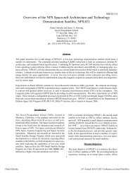
This paper describes the design and performance verification of a magnetically controlled smallsat being built by 

students and staff at the Naval Postgraduate School. The spacecraft (NPSAT1) will carry a number of experiments, 

including two sponsored by the Naval Research Lab and a commercial, off-the-shelf digital camera. Since NPSAT1 

will be a secondary payload, it must be designed for a large mission box at minimum cost. Attitude control pointing 

requirements are less than 10° and an active magnetic control system is planned. NPSAT1 is manifested on the 

Department of Defense Space Test Program (STP) MLV-05, Delta IV mission, due to launch in January 2006. 

Many spacecraft have employed magnetic sensing and actuation for attitude control. However, in most instances, 

the systems are designed with long gravity gradient booms for pitch and roll stabilization. The systems usually 

employ an extended Kalman filter when active damping is required. The NPSAT1 design employs a magnetic 

control system based on favorable moments of inertia realized by optimum equipment placement and ballast. The 

control system uses a standard quaternion control law for attitude control with a linear reduced order estimator for 

rate information. Attitude capture from initial orbit injection rates and steady state attitude errors less than 2° are 

demonstrated by simulation. The simulation is based on an 8th order magnetic field model and includes onboard 

computer sampling, torque rod command quantization, lag and saturation. Sensing and torque events are separated 

in time to prevent contamination of magnetometer data. Air bearing tests are planned for final performance 

verification. The control system hardware and software represent a minimum cost approach to spacecraft attitude 

control. 

b = normalized magnetic field in orbit frame 

B = normalized magnetic field in body frame 

Bdot = derivative of B with respect to time 

Bt = Km B ~Tesla 

Bx,By,Bz = body frame components of B 

B 2 = magnitude squared of B 

gx, gy, gz = actuator time average gains 

Ix, Iy, Iz = principal moments of inertia 

k = Bdot gain 

K = controller gain, [Ka Kb] (3x6) 

Km = field “dipole strength”~Tesla 

Lr = reduced order estimator gain (3x3) 

mp = magnetic moment produced 

mr = magnetic moment requested 

q1 q2 q3 q4 = quaternion elements 

Tp = torque produced by the torque rods 

Nomenclature 

x = state vector (= ~ ϕθψϕθψ) 

, , , , , 

y = measurement vector (= ~ ϕθψ) , , 

Tr = torque requested by the control law 

u = control vector 

α = true anomaly 

β = angle between sun and the orbit plane 

Γ = density variation factor 

ν = orbit angle WRT the sub-solar point 

ρ, ρo, ρmax = atmospheric density, average and max 

ϕθψ , , = yaw, pitch, roll Euler angle sequence 

ω = angular velocity WRT orbit frame 

ωe = spin rate of Earth 

ωn = line of nodes regression rate 

ωo = orbit angular velocity 

1 

16 th Annual AIAA/USU Conference on Small Satellites


Introduction 

Many control system actuator options are available to 

the spacecraft designer. 1,2 This paper considers only 

magnetic actuators because of their compatibility with 

smallsats. The sensing options considered include 

magnetometers, sun sensors, horizon sensors and 

MEMS gyros. Six options using various combinations 

of these sensors have been evaluated in a simulation 

using an IGRF 1,3,4 magnetic field of 8 th degree. All of 

the options meet NPSAT1 pointing requirement of less 

than 10º. The performance of each option would be 

enhanced by the addition of an ideal gravity gradient 

boom. The ideal boom would act as a rigid body in the 

presence satellite librations and thermal distortion. The 

selected option requires only magnetometers and 

magnetic torquers and does not require a boom at the 

560 km mission altitude. The rigid body moments of 

inertia are modified by ballast to avoid resonance with 

the aero and solar disturbance torques at orbital 

frequency. This magnetic control approach does 

require an on board orbit propagator and tracking data 

on a weekly basis to meet pointing requirements. The 

selected control law is based on deriving rate from 

magnetometer data using a reduced order estimator 5 and 

time average 6 linearization of the torque rod control 

law. 2 This time average linearization enhances the 

application of linear analysis techniques. Consequently, 

an LQR approach is used to derive controller gains. 

Estimator gain selection is guided by simulation results. 

This approach is compared with a pole placement 

approach in the Appendix for the baseline spacecraft, a 

spacecraft with Ix slightly greater than Iy and for a 

spacecraft with a short boom. The transient response 

and steady errors of all three spacecraft are acceptable 

for this application. The controller and estimator gain 

calculations for all three spacecraft are based on a 

combined LQR pole placement approach. 

The paper is presented in four sections. Section 1 

describes the control system operation and design. 

Section 2 describes the system simulation. Section 3 

presents simulation results and includes a performance 

comparison with options employing addition sensors. 

Section 4 discusses an error analysis of the baseline all 

magnetic system. The Appendix includes simulation 

details and the gain selection process. 

I. Control System Description 

The baseline control system functional block diagram is 

shown in Fig. 1. Ephemeris data is used to calculate 

components of the magnetic field vector b in orbital 

coordinates based on the International Geomagnetic 

Reference Field (IGRF of 8 th degree.) 

Actuator 

Ctrl Law 

Fig. 1 Control system functional block diagram 

An ideal quaternion control law 2 

u = 2 Ka y + Kb w (1) 

(where y = 2[q1q4 q2q4 q3q4] T ) requires three axis 

attitude information from several sensors or extensive 

filtering of magnetometer data. Accurate calculation of 

w ?from magnetometer data is nontrivial. 7,8 An 

approximation for y, obtained directly from 

magnetometers and ephemeris data is given by: 7,8 

Eq. (2) can be viewed as a cross product steering law. 

The reduced order estimator 5 (ROE) uses this 

measurement, y, to estimate the state vector, x. 

Selection of the gain K and the estimator gain Lr is 

described in the Appendix. Simulation data comparing 

the ideal and approximate approaches is presented in a 

later section.? The actuator control law is given by 2 

(2) 

mr = Tr x B / B 2 (3) 

and the torque on the spacecraft is given by 2 

Tp = mp x B (4) 

In the linear range of the magnetic torquers (i.e., when 

mp = mr), it can be shown that Tp = B Tr 

2 

T r 

1./(gx gy gz) 

u 

-K 

B 

. . 

m r 

~ 

x 

PWM 

k 

Red. Ord. 

Estimator 

B dot 

d/dt 

Magnetometer 

Bxb ^ ^ 

2 

Clock 

y 

~ 

= B 

^ 

x 

^ ~ 

T 

b / 2 = 2[q1q4 q2q4 q3q4] 

y 

B 

b 

Ephemeris 

& b Calc. 


where, 

B = 


(By 2 + Bz 2 )/B 2 -BxBy/ B 2 -BxBz/ B 2 

-BxBy/ B 2 (Bx 2 + Bz 2 )/B 2 -ByBz/ B 2 

-BxBz/ B 2 -ByBz/ B 2 (Bx 2 + By 2 )/B 2 

The off diagonal terms of B have an average value of 

zero. 6 The diagonal terms, defined as gx, gy, and gz 

respectively have average values that are a function of 

orbit inclination. 6 This dependence is shown in Table 1. 

Multiplying the components of Tr by the reciprocals of 

gx, gy, and gz, respectively, yields an average value of 

Tp equal to Tr (i.e.; an ideal actuator, on the average). 

These gains influence performance of the controller and 

estimator gain selection process. 

Table 1 Actuator Average Gains Versus 

Inclination at 560 km (IGRF 2000) 

Inc. g x g y g z Inc. g x g y g z 

0 0.967 0 0.804 60 0.739 0.857 0.39 

10 0.995 0.068 0.781 70 0.709 0.923 0.353 

20 0.922 0.256 0.711 80 0.691 0.965 0.335 

30 0.876 0.46 0.614 90 0.686 0.981 0.333 

40 0.826 0.632 0.522 100 0.691 0.965 0.335 

50 0.78 0.762 0.446 110 0.709 0.923 0.353 

The b vector calculation requires latitude and longitude 

data accurate to approximately 0.1º (about 12 km in 

track). A coarse GPS system would be ideal; however, 

budget constraints forced the evaluation of alternatives. 

The two options being considered are an on-board orbit 

propagator (such as the SGP 9 model) and filtering of 

magnetometer and sun sensor data. 10 The SGP approach 

is currently favored since the code is reasonably 

compact and ground based updates are directly 

compatible with NORAD tracking data. The SGP 

model, with weekly updates from tracking data, should 

provide the required accuracy at the mission altitude of 

560 km. 

II. Simulation Description 

A block diagram of the system simulation is shown in 

Fig. 2. Simulation parameters are summarized in the 

Appendix. The left upper part of the diagram shows the 

dynamics/kinematics being driven by disturbance and 

control torques. 

The upper right part of the diagram shows the 

generation of the circular orbit true anomaly, α=αo+ωot, 

and the location of the Greenwich meridian with respect 

to the right ascension of the ascending node, 

λ=λo+(ωe-?ωn)t. 

Initial simulation work was based on a simple dipole 

model of the Earth’s magnetic field. However, this 

model yielded very optimistic result and was replaced 

by an 8 th degree IGRF model. 

Components of the magnetic field vector are computed 

in latitude and longitude increments of five and ten 

degrees respectively for the mission altitude. This data 

is incorporated in a double look-up table and 

transformed into orbit coordinates of the b vector. The 

Orbit to Body Transformation provides the body frame 

field vector, B. The gravity-gradient, solar and aero 

torques are calculated in the Environmental Torques 

block. The location of the sub-solar point with respect 

to the right ascension of the ascending node, ν=νo+ωot, 

allows calculation of day-night density variation 6 (see 

Appendix). 

The lower part of Fig. 2 shows the spacecraft hardware 

and software. The lower right part of the diagram 

repeats the magnetic field model, discussed above, for 

the purpose of evaluating the impact of ephemeris and 

magnetic field model errors. The lower left part of the 

diagram contains the Torque Rods, Magnetometers and 

the two control modes. The initial control mode, 11 

mr=k Bdot, reduces launch vehicle tip-off rates rapidly. 

The second mode provides attitude capture. Switching 

between modes will be controlled from the ground. 

III. Simulation Results and Comparison of Options 

Fig.3 shows rate and attitude versus time. The upper 

traces are without the Bdot control mode. The center 

traces use Bdot for 10,000 sec. The lower traces use 

Bdot for 20,000 sec. While these results show 

convergence without Bdot, rate damping is clearly 

improved with Bdot. In addition, Bdot convergence to 

low rates can be proven by analysis. 11,12 The Bdot mode 

damps rates but can not accomplish three axis attitude 

pointing. The second mode, referred to as the reduced 

order estimator (ROE) reduces attitude errors to about 

1.5º (erro r primarily due to aero/solar torques). 

The simulation was expanded to examine control 

options using additional sensors. A summary of the 

options and their characteristics is presented in Table 2. 

3 


Body Rates (deg/s) 




8 

6 

4 

2 

0 

-2 

-4 

Body Rates vs Time (w/o Bdot) 

0 1 2 3 4 5 

x 10 4 

-6 

Time (sec) 

Body Rates vs Time (Bdot until 1e4 s) 

8 

6 

4 

2 

0 

-2 

-4 

0 1 2 3 4 5 

x 10 4 

-6 

Time (sec) 

Body Rates vs Time (Bdot until 2e4 s) 

8 

6 

4 

2 

0 

-2 

-4 

T p 

Σ 

m px B t 

m p 

Trq Rod 

& PWM 

m r 

. . 

Trq Rod 

Ctrl Law 

Dynamics, 

Kinematics 

k 

B. 

T r 

d/dt 

K m 

1./ (g x g y g z ) 

DCM 

0 1 2 3 4 5 

x 10 4 

-6 

Time (sec) 

u 

-K 

ROE 

Environmental 

Torques Calc. 

Orbit to body 

x-formation 

y 

B 

Magnet 

-ometer 

^ ^ 

B x b 

2 

Fig. 2 Simulation Block Diagram 

4 

Euler Angles (deg) 



150 

100 

50 

0 

-50 

ouch 

-100 

Euler Angles vs Time (w/o Bdot) 

0 1 2 3 4 5 

x 10 4 

-150 

Time (sec) 

150 

100 

50 

0 

-50 

-100 

Euler Angles vs Time (Bdot until 1e4 s) 

0 1 2 3 4 5 

x 10 4 

-150 

Time (sec) 

Euler Angles vs Time (Bdot until 2e4 s) 

150 

100 

50 

0 

-50 

-100 

Σ 

ν ο 

Fig. 3 Simulation Results 

b 

IGRF 

Look 

Up 

Table 

i 

Lat, 

Lon 

Calc 

i 

0 1 2 3 4 5 

x 10 4 

-150 

Time (sec) 

α 

λ 

α ο 

ω ο 

Σ t 

Clk 

Σ ωe-ωn λ ο 

α ο 

IGRF 

α 

ω 

b Lat, Σ ο 

Look 

t 

Lon 

Clk 

Up 

Σ ωe-ωn Calc 

Table λ 

λ ο 



Table 2 Performance and characteristics of sensing options. 

Option 

Attitude Data Rate Data SS Error Acquisition Option Characteristics 

Day Night ~deg Time~revs* Sensor Suite Power Dcost Dmass 

Option 1 corresponds to the data in the lower part of 

Fig. 3 and uses only magnetometer data. Option 2 

assumes perfect quaternion data during the day but only 

magnetometer data during eclipse. Option 3 assumes 

perfect quaternion data both day and night. All three of 

these options use Bdot, then the ROE. Options 4, 5, and 

6 repeat Options 1, 2 and 3 but the ROE is replaced 

with ideal rate gyros to measure body rates. Clearly, the 

gyros provide better performance; however, they 

require more resources. 

V. Error Sources and Impact 

All of the options mentioned above are subject to errors 

that degrade their steady state accuracy. An error 

analysis of Option 1 is summarized in Table 3. The 

simulation was expanded to evaluate most of the error 

contributors. A modulation approach was used to avoid 

modeling torque rod corruption of magnetometer data. 

The torque rods are used at a 5% duty cycle, every two 

seconds. This provides adequate torque rod decay time 

(approximately 40 time constants). Results indicate an 

RSS error of 3.4º and a worst on worst error of 8.8º. 

While the error analysis requires further verification 

with actual hardware, initial results indicate pointing 

requirements are achievable. 

V. Conclusions 

A low cost control system for small satellites has been 

described. The system requires a three-axis 

magnetometer, three magnetic torque rods and simple 

on board calculations. The system does not require a 

boom or complex filter. Attitude information is derived 

from the cross product of the measured and predicted 

magnetic fields. 7,8 Rate information is derived by 

extending a SISO reduced order estimator 5 to this 

Table 3 Error Analysis Results 

Error Source Allocation Units Error 

MIMO system. Weekly tracking data updates, to the 

SGP orbit propagator, provide a degree of autonomy. 

The system achieves the required pointing accuracy and 

compares favorably with options of greater complexity. 

A process has been outlined for calculation of magnetic 

system controller and estimator gains (see Appendix). 

5 

~W ~K$ ~kg 

1** Mag Mag Estimator 1.5 5 to 24 Mag 1.2 ---- ---- 

2*** Quat Mag 1.3 Mag + SS 1.8 6 0.9 

3 Quat Quat 0.4 Mag + HS 2.2 80 1 

4 Mag Mag Gyros 0.6 4 to 8 Mag + Gyro 4.6 11 0.2 

5 Quat Mag 0.5 Mag+SS+Gyro 5.2 17 1.1 

6 Quat Quat 0.4 Mag+HS+Gyro 5.6 91 1.2 

* Acquisition time is initial condition dependent (attitude, rate, true anomaly and lat./lon.) 

** Magnetometer based control law; *** Quaternion based control law (Mag + SS or HS) 

Δcost = hardware cost only (doesn't include I & T); Mag=magnetometer,SS=Sun senor, HS=horison sensor 

~deg 

Magnetic Field Model* Δ 1.5yrs nT 0.8 

Ephemeris Generator : 12 km 

Latitude Uncertainty 0.1 deg 0.1 

Longitude Uncertainty 0.1 deg 0.1 

Orbit Eccentricity 0.0005 deg 0.07 

Magnetometer: Accuracy ** 0.5 % 0.37 

Alignment 0.25 deg 2 

Linearity ** 0.15 % 0.1 

Noise** 20 pT 0.1 

Orthogonality 0.25 deg 1.7 

Bias** 250 nT 1 

Torque Rod Orthogonality 1 deg 0.05 

Mag Sample / Torque Rod Lag 0.01 sec 0.01 

Ascent Shift 1 mm 0.2 

Disturbance Torques (cm-cp) 8 mm 1.6 

MOI Uncertainty 0.01 kg.m 2 

0.6 

* DGRF vs. IGRF WOW 8.8 

**Billingsley TFM100G2 Spec. RSS 3.42 



Disturbance Torques 

Appendix 

The atmospheric density variation from eclipse to 

sunlight can be expressed as: 6 

? ρ = ρο Γ cosν (A1) 

Eq. (A1) applies when the sun is in the orbit plane (i.e., 

β=0). For nonzero β?, Eq.(A1) has been modified to 

provide a smooth transition from β = 0 to β = pi/2 as 

follows: 

ρ = ρο Γ cosνcosβ (A2) 

Expressing Eq. (A2) in terms of the orbit max density 

(assumed to occur at ν = β= 0) 

ρ = ρmaxΓ (cosνcosβ−1) 

(A3) 

Eq. (A3) was used to calculate aero torques with 

Γ=1.5. 6 Conservative solar torque was also included in 

the simulation. Future work will assess the value of 

incorporating these disturbance torques into the 

estimator. 12 

Simulation Parameters 

The simulation data is summarized in Table A1. 

Table A1 Simulation Parameters 

Parameter & units Value 

Altitude~km 560 

Inclination ~deg 35.4 

Density~kg/m^3 2.21E-13 

Cd 2.5 

Area~cm^2 [ 2674, 2674, 1927] 

(cp-cm)~mm [2, 2, 8] 

Ixx~kg.m^2 5 

Iyy~kg.m^2 5.1 

Izz~kg.m^2 2 

Ixy=Ixz=Iyz (nom.) 0 

k 200 

Km~ Tesla 2.30E-05 

Trqr saturat'n.~ A.m^2 30 

Gain Selection Process 

This section describes three approaches for selecting 

the controller gain, K, and the estimator gain, Lr. The 

design was driven by a requirement to minimize 

response to disturbance torques at orbital frequency. 

The gain selection process actually began by arranging 

equipment within the spacecraft such that favorable 

moments of inertia were achieved (i.e., move the open 

loop roots as far away from ωo as practical). This was 

accomplished while minimizing cross products of 

inertia and the distance between the centers of pressure 

and mass. The average torque gains 6 (gx, gy, gz ) 

provide time average linearization and enhance linear 

analysis techniques. 

The controller gain, K, was initially selected using a 

standard LQR approach to minimize the time integral 

of: 

The matrix Q was selected as the identity matrix. The 

three diagonal elements of R were selected as [1 4 

0.004] to emphasize reduction of the yaw error. The 

REO gain, Lr, was selected as a diagonal matrix. The 

three elements of Lr were varied to achieve maximum 

damping in the presence of noise (a situation analogous 

to the “lead lag” ratio in a SISO system). The resulting 

estimator and controller roots are shown in Table A2. 

Results of a second approach using pole placement are 

also summarized in Table A2. In this approach, the 

controller and estimator gains are calculated with a 

MIMO pole placement routine. Selection of these 

controller poles (round off of the LQR poles) would 

have been difficult without the LQR produced values. 

A third approach combines LQR and pole placement as 

follows: 

Use an LQR routine to select K, with Q as the 6x6 

identity matrix and R as a 3x3 diagonal matrix. Vary 

the three elements of R to achieve best performance for 

reasonable control effort. The LQR routine also outputs 

the three pairs of controller Eigenvalues. Use the norm 

of each pair of these Eigenvalues as a base set of 

estimator poles. Multiply this base set by a factor 

between 6 and 10 (high factors produce greater 

damping but greater noise response). Use the pole 

placement routine to calculate Lr. 

6 

x’Qx+u’Ru 



Table A2 Eigenvalues and Gain Selection 

System Equation Eigenvalues/wo 

LQR * Pole Placem't 

Re part Im part Re part Im part 

Plant A 0 +- 1.687 0 +- 1.687 

0 +-0.2087 0 +-0.2087 

0 +-1.328 0 +-1.328 

Controller A-BK -8.775 +-8.801 -8.8 +-8.8 

-1.054 +-1.876 -1.1 +-1.9 

-0.648 +-1.478 -0.65 +-1.5 

ROE** Abb-LrAab -82.96 0 -74.6 0 

-49.79 0 -13.2 0 

-41.48 0 -9.81 0 

* Q=6x6 identity matrix, R=Diagonal matrix (1 4 0.004), 

Lr=Diagonal matrix (0.09 0.045 0.054) 

**Reduced order estimator: A bb , A ab from partitioned 

A matrix as follows: Abb= rows 4-6, columns 4-6; 

A ab= rows 1-3, columns 4-6. 

A= plant matrix (6x6) ; B= control input matrix (6x3) 

The LQR weighting matrices shown in (Table A2) 

were used with two other sets of moments of inertia, 

namely: [Ix Iy Iz] = [5.7 5.6 2.2] and [20 20 2.2]. No 

adjustment to the simulation was required for the first 

set. Even though Ix>Iy, the results are satisfactory with 

steady state errors only slightly worse (0.1º) than the 

baseline set. The second set, equivalent to adding a 

short boom, required changing the R diagonal matrix to 

(2.1 4 0.0011) to produce comparable results. The 

combined approach still requires some iteration to find 

the best R. However, Lr is calculated by the pole 

placement routine. 

Table A3 LQR / Pole Placement Code 

Q=eye(6); 

[K,S,e]=lqr(A,B,Q,R) 

R=[1 0 0;0 4 0;0 0 .004] 

pe=-6*[norm(e(1)) norm(e(3)) norm(e(5))] 

Lr=place(Abb',Aab',e)' 

Code used in the LQR / Pole Placement approach is 

summarized in Table A3. 

Acknowledgments 

The author acknowledges support from students and 

staff at the Naval Postgraduate School. 

References 

1. Wertz, J. R., “Spacecraft Attitude Determination 

and Control”, Kluwer Academic Publishers, 

Boston, MA, 1994, pp. 779-781 

2. Sidi, M. J., “Spacecraft Dynamics and Control”, 

Cambridge University Press, 1997, p. 129, p. 156. 

3. International Association of Geomagnetism and 

Aeronomy, Division V, Working Group 

4. Revision Of The IGRF for 2000-2005, 

5. Franklin, G. F., Powell, J. D., Emami-Naeini, A., 

“Feedback Control Of Dynamics Systems”, 

Addison Wesley, 1988, pp. 352-356 

6. Martel, F., Pal, P. K., and Psiaki, M., “Active 

Magnetic Control System for Gravity Gradient 

Stabilized Spacecraft”, Second Annual AIAA/USU 

Conference on Small Satellites, (26-28 September 

1988, Logan, UT), Washington, DC: AIAA. 

7. Landiech, Philippe, “Extensive Use of 

Magnetometers and Magnetotorquers for Small 

Satellites Attitude Estimation and Control, 18 th 

Annual AAS Guidance and Control Conference, 

Keystone, Colorado, Feb 1-5, 1995, AAS95-012. 

8. Psiaki, M. L., Martel, F., and Pal, K. P., “Three– 

Axis Attitude Determination via Kalman Filtering 

of Magnetometer Data”, Journal of Guidance, 

Control and Dynamics, Vol. 23, No. 3 pp 506-514. 

9. Hoots, F. R. and Roehrich, R. L., “SPACETRACK 

REPORT NO.3, Models for Propagation of 

NORAD Element Sets”, December 1980, 

Compiled by TS Kelso, 31 Dec 1988. 

10. Jung, H. and Psiaki, M. L., “Tests of 

Magnetometer/Sun Sensor Orbit Determination 

Using Flight Data”, Journal of Guidance, Control 

and Dynamics, Vol.25, No.3 pp. 582-590. 

11. Stickler, C. A. and Alfriend, K. T., “An Elementary 

Magnetic Attitude Control System”, Journal of 

Spacecraft and Rockets, 1976, pp 282-287. 

12. Wisniewski, R., and Blanke, M., “Fully Magnetic 

Attitude Control for Spacecraft Subject to Gravity 

Gradient”, Automatica 35 (1999) pp. 1201-1214. 

7

NPSAT1 Magnetic Attitude Control System - Naval Postgraduate ...

You also want an ePaper? Increase the reach of your titles

Delete template?

Save as template?