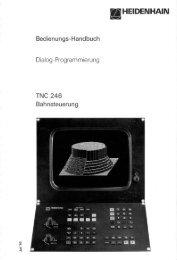
User's Manual TNC 360 (from 259 900-11) - heidenhain
User's Manual TNC 360 (from 259 900-11) - heidenhain
User's Manual TNC 360 (from 259 900-11) - heidenhain

Create successful ePaper yourself
Turn your PDF publications into a flip-book with our unique Google optimized e-Paper software.
May 1994<br />
HEIDENHAIN<br />
<strong>User's</strong> <strong>Manual</strong><br />
HEIDENHAIN Conversational<br />
Programming<br />
<strong>TNC</strong> <strong>360</strong>
Keys and Controls on the <strong>TNC</strong> <strong>360</strong><br />
Controls on the Visual Display Unit<br />
Override Knobs<br />
50<br />
50<br />
Brightness<br />
Machine Operating Modes<br />
Programming Modes<br />
Feed rate<br />
Spindle speed<br />
MANUAL OPERATION<br />
ELECTRONIC HANDWHEEL<br />
POSITIONING WITH MANUAL DATA INPUT<br />
PROGRAM RUN, SINGLE BLOCK<br />
PROGRAM RUN, FULL SEQUENCE<br />
PROGRAMMING AND EDITING<br />
TEST RUN<br />
Program and File Management<br />
PGM<br />
NR<br />
CL<br />
PGM<br />
PGM<br />
CALL<br />
EXT<br />
MOD<br />
Cursor and GOTO keys<br />
GOTO<br />
Graphics<br />
100<br />
0<br />
100<br />
0<br />
MOD<br />
BLK<br />
FORM<br />
MAGN<br />
START<br />
150<br />
F %<br />
150<br />
S %<br />
Select programs and files<br />
Delete programs and files<br />
Enter program call in a program<br />
External data transfer<br />
Supplementary modes<br />
Move cursor (highlight)<br />
Go directly to blocks, cycles and parameter<br />
functions<br />
Graphic operating modes<br />
Define blank form, reset blank form<br />
Magnify detail<br />
Start graphic simulation<br />
Programmable Contours<br />
L<br />
CR<br />
CT<br />
Tool Functions<br />
Straight line<br />
Circle center / Pole for polar coordinates<br />
Circle with center point<br />
Circle with radius<br />
Circle with tangential transition<br />
Corner rounding<br />
Enter or call tool length and radius<br />
Activate tool radius compensation<br />
Cycles, Subprograms and Program Section Repeats<br />
Define and call cycles<br />
Enter and call labels for subprogramming<br />
and program section repeats<br />
Abort an interrupted program run or<br />
enter a program stop in a program<br />
Set a datum with the 3D touch probe or<br />
enter touch probe functions in a program<br />
Entering Numbers and Coordinate Axes, Editing<br />
X<br />
0<br />
.<br />
+/<br />
P<br />
Q<br />
CC<br />
C<br />
RND<br />
TOOL<br />
DEF<br />
R + R<br />
CYCL<br />
DEF<br />
LBL<br />
SET<br />
STOP<br />
TOUCH<br />
PROBE<br />
NO<br />
ENT<br />
ENT<br />
END<br />
CE<br />
DEL<br />
TOOL<br />
CALL<br />
...<br />
...<br />
R- L<br />
CYCL<br />
CALL<br />
LBL<br />
CALL<br />
Q<br />
DEF<br />
IV<br />
9<br />
Select or enter coordinate axes<br />
in a program<br />
Numbers<br />
Decimal point<br />
Algebraic sign<br />
Polar coordinates<br />
Incremental values<br />
Q parameters for part families or<br />
in mathematical functions<br />
Actual position capture<br />
Ignore dialog queries, delete words<br />
Confirm entry and resume dialog<br />
Conclude block<br />
Clear numerical entry<br />
or <strong>TNC</strong> message<br />
Abort dialog; delete program sections
<strong>TNC</strong> Guideline:<br />
From workpiece drawing to<br />
program-controlled machining<br />
Step Task <strong>TNC</strong> Refer to<br />
operating mode Section<br />
Preparation<br />
1 Select tools —— ——<br />
2 Set workpiece datum<br />
for coordinate system —— ——<br />
3 Determine spindle speeds<br />
and feed rates —— 12.4<br />
4 Switch on machine —— 1.3<br />
5 Traverse reference marks or 1.3, 2.1<br />
6 Clamp workpiece —— ——<br />
7 Set the datum /<br />
Reset position display ...<br />
7a ... with the 3D touch probe or 2.5<br />
7b ... without the 3D touch probe or 2.3<br />
Entering and testing part programs<br />
8 Enter part program<br />
or download<br />
over external 5 to 8<br />
data interface or EXT<br />
or 10<br />
9 Test part program for errors 3.1<br />
10 Test run: Run program<br />
block by block without tool 3.2<br />
<strong>11</strong> If necessary: Optimize<br />
part program 5 to 8<br />
Machining the workpiece<br />
12 Insert tool and<br />
run part program 3.2
Sequence of Program Steps<br />
Milling an outside contour<br />
Program step Key Refer to Section<br />
1 Create or select program PGM<br />
4.4<br />
Input: Program number<br />
Unit of measure for programming<br />
NR<br />
2 Define workpiece blank 4.4<br />
3 Define tools 4.2<br />
Input: Tool number<br />
Tool length<br />
Tool radius<br />
4 Call tool data 4.2<br />
Input: Tool number<br />
Spindle axis<br />
Spindle speed<br />
5 Tool change<br />
Input: Coordinates of the tool change position<br />
Radius compensation<br />
Feed rate (rapid traverse)<br />
Miscellaneous function (tool change)<br />
L<br />
e.g. 5.4<br />
6 Move to starting position L<br />
5.2/5.4<br />
Input: Coordinates of the starting position<br />
Radius compensation (R0)<br />
Feed rate (rapid traverse)<br />
Miscellaneous function (spindle on, clockwise)<br />
7 Move tool to (first) working depth<br />
Input: Coordinate of the (first) working depth<br />
Feed rate (rapid traverse)<br />
L<br />
5.4<br />
8 Move to first contour point<br />
Input: Coordinates of the first contour point<br />
Radius compensation for machining<br />
Machining feed rate<br />
if desired, with smooth approach: RND after this block<br />
L<br />
5.2/5.4<br />
9 Machining to last contour point 5 to 8<br />
Input: Enter all necessary values for<br />
each contour element<br />
10 Move to end position<br />
Input: Coordinates of the end position<br />
Radius compensation (R0)<br />
Miscellaneous function (spindle stop)<br />
if desired, with smooth departure: RND after this block<br />
L<br />
5.2/5.4<br />
<strong>11</strong> Retract tool in spindle axis<br />
Input: Coordinates above the workpiece<br />
Feed rate (rapid traverse)<br />
Miscellaneous function (end of program)<br />
L<br />
5.2/5.4<br />
12 End of program<br />
BLK<br />
FORM<br />
TOOL<br />
DEF<br />
TOOL<br />
CALL
How to use this manual<br />
<strong>TNC</strong> <strong>360</strong><br />
This manual describes functions and features available on the <strong>TNC</strong> <strong>360</strong><br />
<strong>from</strong> NC software number <strong>259</strong> <strong>900</strong> <strong>11</strong>.<br />
This manual describes all available <strong>TNC</strong> functions. However, since the<br />
machine builder has modified (with machine parameters) the available<br />
range of <strong>TNC</strong> functions to interface the control to his specific machine,<br />
this manual may describe some functions which are not available on your<br />
<strong>TNC</strong>.<br />
<strong>TNC</strong> functions which are not available on every machine are, for example:<br />
• Probing functions for the 3D touch probe system<br />
• Digitizing<br />
• Rigid tapping<br />
If in doubt, please contact the machine tool builder.<br />
<strong>TNC</strong> programming courses are offered by many machine tool builders as<br />
well as by HEIDENHAIN. We recommend these courses as an effective<br />
way of improving your programming skill and sharing information and<br />
ideas with other <strong>TNC</strong> users.
The <strong>TNC</strong> beginner can use the manual as a workbook. The first part of<br />
the manual deals with the basics of NC technology and describes the <strong>TNC</strong><br />
functions. It then introduces the techniques of conversational programming.<br />
Each new function is thoroughly described when it is first introduced,<br />
and the numerous examples can be tried out directly on the <strong>TNC</strong>.<br />
The <strong>TNC</strong> beginner should work through this manual <strong>from</strong> beginning to end<br />
to ensure that he is capable of fully exploiting the features of this powerful<br />
tool.<br />
For the <strong>TNC</strong> expert, this manual serves as a comprehensive reference<br />
work. The table of contents and cross references enable him to quickly<br />
find the topics and information he needs. Easy-to-read dialog flowcharts<br />
show him how to enter the required data for each function.<br />
The dialog flow charts consist of sequentially arranged instruction boxes.<br />
Each key is illustrated next to an explanation of its function to aid the<br />
beginner when he is performing the operation for the first time. The<br />
experienced user can use the key sequences illustrated in the left part of<br />
the flowchart as a quick overview. The <strong>TNC</strong> dialogs in the instruction<br />
boxes are always presented on a gray background.<br />
Note: Placeholders in the program on the screen for entries which are not<br />
always programmed (such as the abbreviations R, F, M and REP) are not<br />
indicated in the programming examples.<br />
Layout of the dialog flowcharts<br />
Dialog initiation key<br />
L<br />
DIALOG PROMPT (ON <strong>TNC</strong> SCREEN)<br />
e.g.<br />
3 ENT<br />
Answer the prompt with<br />
these keys<br />
NEXT DIALOG QUESTION<br />
Press this key<br />
+/<br />
Or press this key<br />
.<br />
.<br />
.<br />
The functions of the keys are explained here.<br />
Function of the key.<br />
Function of an alternative key.<br />
The trail of dots indicates that:<br />
• the dialog is not fully shown, or<br />
• the dialog continues on the next page.<br />
A dashed line means that either<br />
the key above or below it can be<br />
pressed.<br />
<strong>TNC</strong> <strong>360</strong>
Contents <strong>User's</strong> <strong>Manual</strong> <strong>TNC</strong> <strong>360</strong> (<strong>from</strong> <strong>259</strong> <strong>900</strong>-xx)<br />
Introduction<br />
<strong>Manual</strong> Operation and Setup<br />
Test Run and Program Run<br />
Programming<br />
Programming Tool Movements<br />
Subprograms and Program Section Repeats<br />
Programming with Q Parameters<br />
Cycles<br />
Digitizing 3D Surfaces<br />
External Data Transfer<br />
MOD-Functions<br />
Tabels and Overviews<br />
1<br />
2<br />
3<br />
4<br />
5<br />
6<br />
7<br />
8<br />
9<br />
10<br />
<strong>11</strong><br />
12
1 Introduction<br />
<strong>TNC</strong> <strong>360</strong><br />
1.1 The <strong>TNC</strong> <strong>360</strong> .............................................................................................. 1-2<br />
The Operating Panel ....................................................................................................... 1-3<br />
The Screen ..................................................................................................................... 1-3<br />
<strong>TNC</strong> Accessories ............................................................................................................ 1-5<br />
1.2 Fundamentals of Numerical Control (NC) .............................................. 1-6<br />
Introduction .................................................................................................................... 1-6<br />
What is NC? ................................................................................................................... 1-6<br />
The part program ............................................................................................................ 1-6<br />
Conversational programming ......................................................................................... 1-6<br />
Reference system .......................................................................................................... 1-7<br />
Cartesian coordinate system .......................................................................................... 1-7<br />
Additional axes ............................................................................................................... 1-8<br />
Polar coordinates ............................................................................................................ 1-8<br />
Setting a pole at circle center CC ................................................................................... 1-9<br />
Setting the datum ........................................................................................................... 1-9<br />
Absolute workpiece positions ........................................................................................ 1-<strong>11</strong><br />
Incremental workpiece positions ................................................................................... 1-<strong>11</strong><br />
Programming tool movements ....................................................................................... 1-13<br />
Position encoders ........................................................................................................... 1-13<br />
Reference marks ............................................................................................................ 1-13<br />
1.3 Switch-On ................................................................................................. 1-14<br />
1.4 Graphics and Status Display ................................................................... 1-15<br />
Plan view ........................................................................................................................ 1-15<br />
Projection in three planes ............................................................................................... 1-16<br />
3D view ......................................................................................................................... 1-16<br />
Status Display ................................................................................................................. 1-18<br />
1.5 Programs ................................................................................................... 1-19<br />
Program directory ........................................................................................................... 1-19<br />
Selecting, erasing and protecting programs ................................................................... 1-20
2 <strong>Manual</strong> Operation and Setup<br />
<strong>TNC</strong> <strong>360</strong><br />
2.1 Moving the Machine Axes ....................................................................... 2-2<br />
Traversing with the machine axis direction buttons ....................................................... 2-2<br />
Traversing with the electronic handwheel ..................................................................... 2-3<br />
Working with the HR330 Electronic Handwheel ............................................................ 2-3<br />
Incremental jog positioning ............................................................................................ 2-4<br />
Positioning with manual data input (MDI) ...................................................................... 2-4<br />
2.2 Spindle Speed S, Feed Rate F and Miscellaneous Functions M .......... 2-5<br />
To enter the spindle speed S ......................................................................................... 2-5<br />
To enter the miscellaneous function M .......................................................................... 2-6<br />
To change the spindle speed S ...................................................................................... 2-6<br />
To change the feed rate F .............................................................................................. 2-6<br />
2.3 Setting the Datum Without a 3D Touch Probe...................................... 2-7<br />
Setting the datum in the tool axis .................................................................................. 2-7<br />
To set the datum in the working plane ........................................................................... 2-8<br />
2.4 3D Touch Probe Systems ......................................................................... 2-9<br />
3D Touch probe applications .......................................................................................... 2-9<br />
To select the touch probe menu .................................................................................... 2-9<br />
Calibrating the 3D Touch Probe ...................................................................................... 2-10<br />
Compensating workpiece misalignment ........................................................................ 2-12<br />
2.5 Setting the Datum with the 3D Touch Probe System .......................... 2-14<br />
To set the datum in a specific axis ................................................................................. 2-14<br />
Corner as datum ............................................................................................................. 2-15<br />
Circle center as datum ................................................................................................... 2-17<br />
2.6 Measuring with the 3D Touch Probe System ........................................ 2-19<br />
Finding the coordinate of a position on an aligned workpiece ....................................... 2-19<br />
Finding the coordinates of a corner in the working plane .............................................. 2-19<br />
Measuring workpiece dimensions ................................................................................. 2-20<br />
Measuring angles ........................................................................................................... 2-21
3 Test Run and Program Run<br />
<strong>TNC</strong> <strong>360</strong><br />
3.1 Test Run .................................................................................................... 3-2<br />
To do a test run .............................................................................................................. 3-2<br />
3.2 Program Run ............................................................................................. 3-3<br />
To run a part program ..................................................................................................... 3-3<br />
Interrupting machining ................................................................................................... 3-4<br />
Resuming program run after an interruption .................................................................. 3-5<br />
3.3 Blockwise Transfer: Executing Long Programs ..................................... 3-6
4 Programming<br />
<strong>TNC</strong> <strong>360</strong><br />
4.1 Editing part programs .............................................................................. 4-2<br />
Layout of a program ....................................................................................................... 4-2<br />
Plain language dialog ...................................................................................................... 4-2<br />
Editing functions ............................................................................................................. 4-3<br />
4.2 Tools .......................................................................................................... 4-5<br />
Determining tool data ..................................................................................................... 4-5<br />
Entering tool data into the program ................................................................................ 4-7<br />
Entering tool data in program 0 ...................................................................................... 4-8<br />
Calling tool data .............................................................................................................. 4-9<br />
Tool change .................................................................................................................... 4-10<br />
4.3 Tool Compensation Values ..................................................................... 4-<strong>11</strong><br />
Effect of tool compensation values ................................................................................ 4-<strong>11</strong><br />
Tool radius compensation .............................................................................................. 4-12<br />
Machining corners .......................................................................................................... 4-14<br />
4.4 Program Creation ..................................................................................... 4-15<br />
To create a new part program ........................................................................................ 4-15<br />
Defining the blank form – BLK FORM ............................................................................ 4-15<br />
4.5 Entering Tool-Related Data ..................................................................... 4-16<br />
Feed Rate F .................................................................................................................... 4-16<br />
Spindle speed S .............................................................................................................. 4-17<br />
4.6 Entering Miscellaneous Functions and STOP ........................................ 4-18<br />
4.7 Actual Position Capture ........................................................................... 4-19
5 Programming Tool Movements<br />
<strong>TNC</strong> <strong>360</strong><br />
5.1 General Information on Programming Tool Movements ..................... 5-2<br />
5.2 Contour Approach and Departure .......................................................... 5-4<br />
Starting and end positions .............................................................................................. 5-4<br />
Smooth approach and departure .................................................................................... 5-6<br />
5.3 Path Functions ......................................................................................... 5-7<br />
General information ........................................................................................................ 5-7<br />
Machine axis movement under program control ........................................................... 5-7<br />
Overview of path functions ............................................................................................ 5-8<br />
5.4 Path Contours – Cartesian Coordinates ................................................. 5-9<br />
Straight line .................................................................................................................... 5-9<br />
Chamfer ......................................................................................................................... 5-12<br />
Circle and circular arcs.................................................................................................... 5-14<br />
Circle Center CC ............................................................................................................. 5-15<br />
Circular Path C Around the Center Circle CC ................................................................. 5-17<br />
Circular path CR with defined radius .............................................................................. 5-20<br />
Circular path CT with tangential connection ................................................................... 5-23<br />
Corner rounding RND ..................................................................................................... 5-25<br />
5.5 Path Contours – Polar Coordinates ......................................................... 5-27<br />
Polar coordinate origin: Pole CC ..................................................................................... 5-27<br />
Straight line LP ............................................................................................................... 5-27<br />
Circular path CP around pole CC .................................................................................... 5-30<br />
Circular path CTP with tangential connection................................................................. 5-32<br />
Helical interpolation ........................................................................................................ 5-33<br />
5.6 M-Functions for Contouring Behavior and Coordinate Data ............... 5-36<br />
Smoothing corners: M90 ................................................................................................ 5-36<br />
Machining small contour steps: M97 ............................................................................. 5-37<br />
Machining open contours: M98 ..................................................................................... 5-38<br />
Progamming machine-reference coordinates: M91/M92 ............................................... 5-39<br />
5.7 Positioning with <strong>Manual</strong> Data Input (MDI) ............................................ 5-40
6 Subprograms and Program Section Repeats<br />
<strong>TNC</strong> <strong>360</strong><br />
6.1 Subprograms ............................................................................................ 6-2<br />
Principle ......................................................................................................................... 6-2<br />
Operating limits .............................................................................................................. 6-2<br />
Programming and calling subprograms .......................................................................... 6-3<br />
6.2 Program Section Repeats ........................................................................ 6-5<br />
Principle ......................................................................................................................... 6-5<br />
Programming notes ........................................................................................................ 6-5<br />
Programming and calling a program section repeat ....................................................... 6-5<br />
6.3 Main Program as Subprogram ................................................................ 6-8<br />
Principle ......................................................................................................................... 6-8<br />
Operating limits .............................................................................................................. 6-8<br />
Calling a main program as a subprogram ....................................................................... 6-8<br />
6.4 Nesting ...................................................................................................... 6-9<br />
Nesting depth ................................................................................................................. 6-9<br />
Subprogram in a subprogram ......................................................................................... 6-9<br />
Repeating program section repeats ............................................................................... 6-<strong>11</strong><br />
Repeating subprograms ................................................................................................. 6-12
7 Programming with Q Parameters<br />
<strong>TNC</strong> <strong>360</strong><br />
7.1 Part Families – Q Parameters Instead of Numerical Values ................. 7-3<br />
7.2 Describing Contours Through Mathematical Functions....................... 7-5<br />
Overview ........................................................................................................................ 7-5<br />
7.3 Trigonometric Functions ......................................................................... 7-7<br />
Overview ........................................................................................................................ 7-7<br />
7.4 If-Then Operations with Q Parameters .................................................. 7-8<br />
Jumps ......................................................................................................................... 7-8<br />
Overview ........................................................................................................................ 7-8<br />
7.5 Checking and Changing Q Parameters ................................................... 7-10<br />
7.6 Output of Q Parameters and Messages ................................................. 7-<strong>11</strong><br />
Displaying error messages ............................................................................................. 7-<strong>11</strong><br />
Output through an external data interface ..................................................................... 7-<strong>11</strong><br />
Assigning values for the PLC ......................................................................................... 7-<strong>11</strong><br />
7.7 Measuring with the 3D Touch Probe During Program Run.................. 7-12<br />
7.8 Example for Exercise ................................................................................ 7-14<br />
Rectangular pocket with corner rounding and tangential approach ............................... 7-14<br />
Bolt hole circle ................................................................................................................ 7-15<br />
Ellipse ......................................................................................................................... 7-17<br />
Three-dimensional machining (machining a hemisphere with an end mill) .................... 7-19
8 Cycles<br />
<strong>TNC</strong> <strong>360</strong><br />
8.1 General Overview of Cycles .................................................................... 8-2<br />
Programming a cycle ...................................................................................................... 8-2<br />
Dimensions in the tool axis ............................................................................................ 8-4<br />
Customized macros ........................................................................................................ 8-4<br />
8.2 Simple Fixed Cycles.................................................................................. 8-5<br />
PECKING (Cycle 1) ......................................................................................................... 8-5<br />
TAPPING with floating tap holder (Cycle 2) .................................................................... 8-7<br />
RIGID TAPPING (Cycle 17) ............................................................................................. 8-9<br />
SLOT MILLING (Cycle 3) ................................................................................................ 8-10<br />
POCKET MILLING (Cycle 4) ........................................................................................... 8-12<br />
CIRCULAR POCKET MILLING (Cycle 5) ......................................................................... 8-14<br />
8.3 SL Cycles ................................................................................................... 8-16<br />
CONTOUR GEOMETRY (Cycle 14) ................................................................................ 8-17<br />
ROUGH-OUT (Cycle 6) ................................................................................................... 8-18<br />
SL Cycles: Overlapping contours ................................................................................... 8-20<br />
PILOT DRILLING (Cycle 15) ........................................................................................... 8-26<br />
CONTOUR MILLING (Cycle 16 ...................................................................................... 8-27<br />
8.4 Cycles for Coordinate Transformations ................................................. 8-30<br />
DATUM SHIFT (Cycle 7) ................................................................................................. 8-31<br />
MIRROR IMAGE (Cycle 8) .............................................................................................. 8-33<br />
ROTATION (Cycle 10) ..................................................................................................... 8-35<br />
SCALING FACTOR (Cycle <strong>11</strong>) ........................................................................................ 8-36<br />
8.5 Other Cycles .............................................................................................. 8-38<br />
DWELL TIME (Cycle 9) ................................................................................................... 8-38<br />
PROGRAM CALL (Cycle 12) ........................................................................................... 8-38<br />
ORIENTED SPINDLE STOP (Cycle 13) ........................................................................... 8-39
9 Digitizing 3D Surfaces<br />
<strong>TNC</strong> <strong>360</strong><br />
9.1 The Digitizing Process .............................................................................. 9-2<br />
Generating programs with digitized data ........................................................................ 9-2<br />
Overview: Digitizing cycles ............................................................................................ 9-2<br />
Transferring digitized data .............................................................................................. 9-2<br />
9.2 Digitizing Range ....................................................................................... 9-3<br />
Input data ....................................................................................................................... 9-3<br />
Setting the scanning range ............................................................................................. 9-3<br />
9.3 Line-By-Line Digitizing ............................................................................. 9-5<br />
Starting position ............................................................................................................. 9-5<br />
Contour approach ........................................................................................................... 9-5<br />
Input data ....................................................................................................................... 9-5<br />
Setting the digitizing parameters .................................................................................... 9-6<br />
9.4 Contour Line Digitizing ............................................................................ 9-8<br />
Starting position ............................................................................................................. 9-8<br />
Contour approach ........................................................................................................... 9-8<br />
Input data ....................................................................................................................... 9-8<br />
Limits of the scanning range .......................................................................................... 9-9<br />
Setting the digitizing parameters .................................................................................... 9-9<br />
9.5 Using Digitized Data in a Part Program ................................................. 9-<strong>11</strong><br />
Executing a part program <strong>from</strong> digitized data................................................................. 9-12
10 External Data Transfer<br />
<strong>TNC</strong> <strong>360</strong><br />
10.1 Menu for External Data Transfer ............................................................. 10-2<br />
Blockwise transfer .......................................................................................................... 10-2<br />
10.2 Pin Layout and Connecting Cable for the Data Interface ..................... 10-3<br />
RS-232-C/V.24 Interface ................................................................................................. 10-3<br />
10.3 Preparing the Devices for Data Transfer ................................................ 10-4<br />
HEIDENHAIN Devices .................................................................................................... 10-4<br />
Non-HEIDENHAIN devices ............................................................................................. 10-4
<strong>11</strong> MOD Functions<br />
<strong>TNC</strong> <strong>360</strong><br />
<strong>11</strong>.1 Selecting, Changing and Exiting the MOD Functions........................... <strong>11</strong>-2<br />
<strong>11</strong>.2 NC and PLC Software Numbers .............................................................. <strong>11</strong>-2<br />
<strong>11</strong>.3 Entering the Code Number...................................................................... <strong>11</strong>-3<br />
<strong>11</strong>.4 Setting the External Data Interfaces ...................................................... <strong>11</strong>-3<br />
BAUD RATE ................................................................................................................... <strong>11</strong>-3<br />
RS-232-C Interface ......................................................................................................... <strong>11</strong>-3<br />
<strong>11</strong>.5 Machine-Specific User Parameters ......................................................... <strong>11</strong>-4<br />
<strong>11</strong>.6 Position Display Types ............................................................................. <strong>11</strong>-4<br />
<strong>11</strong>.7 Unit of Measurement ............................................................................... <strong>11</strong>-5<br />
<strong>11</strong>.8 Programming Language .......................................................................... <strong>11</strong>-5<br />
<strong>11</strong>.9 Axes for L Block <strong>from</strong> Actual Position Capture ..................................... <strong>11</strong>-5<br />
<strong>11</strong>.10 Axis Traverse Limits ................................................................................. <strong>11</strong>-6
12 Tables, Overviews, Diagrams<br />
<strong>TNC</strong> <strong>360</strong><br />
12.1 General User Parameters ......................................................................... 12-2<br />
Selecting the general user parameters .......................................................................... 12-2<br />
Parameters for external data transfer............................................................................. 12-2<br />
Parameters for 3D Touch Probes ................................................................................... 12-4<br />
Parameters for <strong>TNC</strong> Displays and the Editor .................................................................. 12-4<br />
Parameters for machining and program run ................................................................... 12-7<br />
Parameters for override behavior and electronic handwheel ......................................... 12-9<br />
12.2 Miscellaneous Functions (M Functions) ................................................. 12-<strong>11</strong><br />
Miscellaneous functions with predetermined effect...................................................... 12-<strong>11</strong><br />
Vacant miscellaneous functions ..................................................................................... 12-12<br />
12.3 Preassigned Q-Parameter ........................................................................ 12-13<br />
12.4 Diagrams for Machining .......................................................................... 12-15<br />
Spindle speed S .............................................................................................................. 12-15<br />
Feed rate F ..................................................................................................................... 12-16<br />
Feed rate F for tapping ................................................................................................... 12-17<br />
12.5 Features, Specifications and Accessories .............................................. 12-18<br />
<strong>TNC</strong> <strong>360</strong> ......................................................................................................................... 12-18<br />
Accessories .................................................................................................................... 12-20<br />
12.6 <strong>TNC</strong> Error Messages ................................................................................. 12-21<br />
<strong>TNC</strong> error messages during programming ..................................................................... 12-21<br />
<strong>TNC</strong> error messages during test run and program run................................................... 12-22<br />
<strong>TNC</strong> error messages with digitizing ............................................................................... 12-25
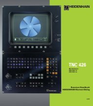
1 Introduction<br />
1.1 The <strong>TNC</strong> <strong>360</strong><br />
1-2<br />
Control<br />
The <strong>TNC</strong> <strong>360</strong> is a shop-floor programmable contouring control for milling<br />
machines, boring machines and machining centers with up to four axes.<br />
The spindle can be rotated to a given angular stop position (oriented<br />
spindle stop).<br />
Visual display unit and operating panel<br />
The monochrome screen clearly displays all information necessary for<br />
operating the <strong>TNC</strong>. In addition to the CRT monitor (BE 212), the <strong>TNC</strong> <strong>360</strong><br />
can also be used with a flat luminescent screen (BF <strong>11</strong>0). The keys on the<br />
operating panel are grouped according to their functions. This<br />
simplifies programming and the application of the <strong>TNC</strong> functions.<br />
Programming<br />
The <strong>TNC</strong> <strong>360</strong> is programmed directly at the machine with the easy to<br />
understand HEIDENHAIN plain language dialog format. Programming in<br />
ISO or in DNC mode is also possible.<br />
Graphics<br />
The graphic simulation feature allows programs to be tested before actual<br />
machining. Various types of graphic representation can be selected.<br />
Compatibility<br />
Any part program can be run on the <strong>TNC</strong> <strong>360</strong> as long as the commands in<br />
the program are within the functional scope of the <strong>TNC</strong> <strong>360</strong>.<br />
<strong>TNC</strong> <strong>360</strong>
1 Introduction<br />
1.1 The <strong>TNC</strong> <strong>360</strong><br />
The Operating Panel<br />
The keys on the <strong>TNC</strong> operating panel are identified with easy-toremember<br />
abbreviations and symbols. The keys are grouped according<br />
to function:<br />
• External data transfer<br />
• Probing functions<br />
• Editing functions<br />
• GOTO statement<br />
• Arrow keys<br />
• STOP key<br />
• Programming of cycles,<br />
program section repeats<br />
and subprograms<br />
• NO ENT key<br />
• Tool-related entries<br />
Graphic operating<br />
modes<br />
• Program selection<br />
• Path function keys<br />
50<br />
PGM<br />
NR<br />
CR<br />
EXT<br />
GOTO<br />
STOP<br />
NO<br />
ENT<br />
MOD<br />
100<br />
0<br />
CL<br />
PGM<br />
RND<br />
TOUCH<br />
PROBE<br />
CYCL<br />
DEF<br />
TOOL<br />
DEF<br />
BLK<br />
FORM<br />
150<br />
F %<br />
PGM<br />
CALL<br />
CT<br />
DEL<br />
CYCL<br />
CALL<br />
TOOL<br />
CALL<br />
GRAPHICS<br />
CC<br />
MAGN START<br />
50<br />
LBL<br />
SET<br />
R- L<br />
Override controls<br />
for spindle speed<br />
and feed rate<br />
100<br />
0<br />
L<br />
C<br />
ENT<br />
LBL<br />
CALL<br />
R + R<br />
7 8 9<br />
4 5 6<br />
1 2 3<br />
<strong>TNC</strong> <strong>360</strong> 1-3<br />
150<br />
S %<br />
X<br />
Y<br />
Z<br />
IV<br />
CE<br />
0<br />
Q<br />
MOD<br />
.<br />
Q<br />
DEF<br />
P<br />
HEIDENHAIN<br />
+/<br />
END<br />
• Numerical entries<br />
• Axis selection<br />
• Q parameter<br />
programming<br />
• Operating modes<br />
• Incremental and<br />
polar coordinates<br />
The functions of the individual keys are described<br />
on the inside front cover.<br />
The machine operating buttons, such as for NC start, are described in the manual for your machine tool.<br />
In this manual they are shown in gray.<br />
The Screen<br />
I<br />
Header<br />
The header of the screen shows the selected operating mode. Dialog<br />
questions and <strong>TNC</strong> messages also appear there.<br />
Brightness control<br />
(BE 212 only)
1 Introduction<br />
1.1 The <strong>TNC</strong> <strong>360</strong><br />
1-4<br />
Screen Layout<br />
MANUAL and EL. HANDWHEEL operating modes:<br />
• Coordinates<br />
• Selected axis<br />
• * means: control<br />
is in operation<br />
• Status display,<br />
e.g. feed rate F,<br />
miscellaneous<br />
function M<br />
Section of<br />
selected<br />
program<br />
Status display<br />
A machine operating mode has been selected<br />
A program run operating mode has been selected<br />
The screen layout is the same in the operating modes PROGRAM RUN,<br />
PROGRAMMING AND EDITING and TEST RUN. The current block is<br />
surrounded by two horizontal lines.<br />
<strong>TNC</strong> <strong>360</strong>
1 Introduction<br />
1.1 The <strong>TNC</strong> <strong>360</strong><br />
<strong>TNC</strong> Accessories<br />
3D Probe Systems<br />
The <strong>TNC</strong> features the following functions for the<br />
HEIDENHAIN 3D touch probe systems:<br />
• Automatic workpiece alignment (compensation<br />
of workpiece misalignment)<br />
• Datum setting<br />
• Measurements of the workpiece can be performed<br />
during program run<br />
• Digitizing 3D forms (optional)<br />
The TS 120 touch probe system is connected to the<br />
control via cable, while the TS 510 communicates<br />
by means of infrared light.<br />
Floppy Disk Unit<br />
The HEIDENHAIN FE 401 floppy disk unit serves as<br />
an external memory for the <strong>TNC</strong>, allowing you to<br />
store your programs externally on diskette.<br />
The FE 401 can also be used to transfer programs<br />
that were written on a PC into the <strong>TNC</strong>. Extremely<br />
long programs which exceed the <strong>TNC</strong>'s memory<br />
capacity are “drip fed” block by block. The machine<br />
executes the transferred blocks and erases them<br />
immediately, freeing memory for further blocks<br />
<strong>from</strong> the FE.<br />
Electronic Handwheels<br />
Electronic handwheels provide precise manual<br />
control of the axis slides. As on conventional<br />
machines, turning the handwheel moves the axis<br />
by a defined amount. The traverse distance per<br />
revolution of the handwheel can be adjusted over a<br />
wide range.<br />
Portable handwheels, such as the HR 330, are<br />
connected to the <strong>TNC</strong> by cable. Built-in handwheels,<br />
such as the HR 130, are built into the<br />
machine operating panel.<br />
An adapter allows up to three handwheels to be<br />
connected simultaneously. Your machine manufacturer<br />
can tell you more about the handwheel<br />
configuration of your machine.<br />
Fig. 1.5: HEIDENHAIN 3D Probe Systems TS 120 and TS 5<strong>11</strong><br />
Fig. 1.6: HEIDENHAIN FE 401 Floppy Disk Unit<br />
Fig. 1.7: The HR 330 Electronic Handwheel<br />
<strong>TNC</strong> <strong>360</strong> 1-5
1 Introduction<br />
1.2 Fundamentals of Numerical Control (NC)<br />
Introduction<br />
1-6<br />
This chapter addresses the following topics:<br />
• What is NC?<br />
• The part program<br />
• Conversational programming<br />
• Cartesian coordinate system<br />
• Additional axes<br />
• Polar coordinates<br />
• Setting a pole at a circle center (CC)<br />
• Datum setting<br />
• Absolute workpiece positions<br />
• Programming tool movements<br />
• Position encoders<br />
• Reference mark evaluation<br />
What is NC?<br />
NC stands for Numerical Control. Simply put, numerical control is the<br />
operation of a machine by means of coded instructions. Modern controls<br />
such as the HEIDENHAIN <strong>TNC</strong>s have a built-in computer for this purpose.<br />
Such a control is therefore also called a CNC (Computer Numerical<br />
Control).<br />
The part program<br />
A part program is a complete list of instructions for machining a workpiece.<br />
It contains such information as the target position of a tool movement,<br />
the tool path — i.e. how the tool should move towards the target<br />
position — and the feed rate. The program must also contain information<br />
on the radius and length of the tools, the spindle speed and the tool axis.<br />
Conversational programming<br />
Conversational programming is a particularly easy way of writing and<br />
editing part programs. From the very beginning, HEIDENHAIN numerical<br />
controls were designed for the machinist who keys in his programs<br />
directly at the machine. This is why they are called <strong>TNC</strong>s, or "Touch<br />
Numerical Controls."<br />
You begin programming each machining step by simply pressing a key.<br />
The control then asks for all further information required to execute the<br />
step. You can also program the <strong>TNC</strong> in ISO format or download programs<br />
<strong>from</strong> a central host computer for DNC operation.<br />
<strong>TNC</strong> <strong>360</strong>
1 Introduction<br />
1.2 Fundamentals of NC<br />
Reference system<br />
In order to define positions, one needs a reference system. For example,<br />
positions on the earth's surface can be defined "absolutely" by their<br />
geographic coordinates of longitude and latitude. The term "coordinate"<br />
comes <strong>from</strong> the Latin word for "that which is arranged". The network of<br />
horizontal and vertical lines around the globe constitute an "absolute<br />
reference system" — in contrast to the "relative" definition of a position<br />
that is referenced, for example, to some other, known location.<br />
Cartesian coordinate system<br />
A workpiece is normally machined on a <strong>TNC</strong> controlled milling machine<br />
according to a workpiece-reference Cartesian coordinate system (a<br />
rectangular coordinate system named after the French mathematician and<br />
philosopher Renatus Cartesius; 1596 to 1650). The Cartesian<br />
coordinate system is based on three coordinate axes X, Y and Z, which are<br />
parallel to the machine guideways. The figure to the right illustrates the<br />
"right hand rule" for remembering the three axis directions: the<br />
middle finger is pointing in the positive direction of the tool axis <strong>from</strong> the<br />
workpiece toward the tool (the Z axis), the thumb is pointing in the<br />
positive X direction, and the index finger in the positive Y direction.<br />
<strong>TNC</strong> <strong>360</strong> 1-7<br />
90°<br />
Greenwich<br />
0° 90°<br />
60°<br />
60°<br />
30°<br />
0°<br />
30°<br />
Fig. 1.9: The geographic coordinate system<br />
is an absolute reference system<br />
+Y<br />
+Y<br />
+Z<br />
+X<br />
+Z<br />
+X<br />
Fig. 1.10: Designations and directions of the<br />
axes on a milling machine
1 Introduction<br />
1.2 Fundamentals of NC<br />
Additional axes<br />
1-8<br />
The <strong>TNC</strong> can control machines which have more than three axes. U, V<br />
and W are secondary linear axes parallel to the main axes X, Y and Z,<br />
respectively (see illustration). Rotary axes are also possible. They are<br />
designated as axes A, B and C.<br />
Polar coordinates<br />
The Cartesian coordinate system is especially<br />
useful for parts whose dimensions are mutually<br />
perpendicular. But when workpieces contain<br />
circular arcs, or when dimensions are given in<br />
degrees, it is often easier to use polar coordinates.<br />
In contrast to Cartesian coordinates, which are<br />
three-dimensional, polar coordinates can only<br />
describe positions in a plane.<br />
The datum for polar coordinates is the circle<br />
center CC. To describe a position in polar coordinates,<br />
think of a scale whose datum point is rigidly<br />
connected to the pole but which can be freely<br />
rotated in a plane around the pole.<br />
Positions in this plane are defined by:<br />
• Polar Radius (PR): The distance <strong>from</strong> circle<br />
center CC to the defined position.<br />
• Polar Angle (PA): The angle between the<br />
reference axis and the scale.<br />
Y+<br />
10<br />
PR<br />
Fig. 1.<strong>11</strong>: Arrangement and designation of<br />
the auxiliary axes<br />
PA 3<br />
W+<br />
PR<br />
CC<br />
Fig. 1.12: Positions on an arc with polar coordinates<br />
Z<br />
30<br />
PA 2<br />
C+<br />
PR<br />
PA 1<br />
B+<br />
U+<br />
A+<br />
Y<br />
V+<br />
0°<br />
X<br />
X+<br />
<strong>TNC</strong> <strong>360</strong>
1 Introduction<br />
1.2 Fundamentals of NC<br />
Setting a pole at circle center CC<br />
Z<br />
The pole (circle center) is defined by setting two Cartesian coordinates.<br />
These two coordinates also determine the reference axis for the polar<br />
angle PA.<br />
CC<br />
Coordinates of the pole Reference axis of the angle<br />
Y<br />
X Y +X<br />
Y Z +Y<br />
Z X +Z<br />
Fig. 1.13: Polar coordinates and their associated reference axes<br />
Setting the datum<br />
+<br />
0°<br />
X<br />
Z<br />
The workpiece drawing identifies a certain prominent point on the workpiece<br />
(usually a corner) as the "absolute datum" and perhaps one or more<br />
other points as relative datums. The process of datum setting establishes<br />
these points as the origin of the absolute or relative coordi-nate systems:<br />
The workpiece, which is aligned with the machine axes, is moved to a<br />
certain position relative to the tool and the display is set either to zero or<br />
to another appropriate position value (e.g. to compen-sate the tool radius).<br />
CC<br />
+<br />
0°<br />
<strong>TNC</strong> <strong>360</strong> 1-9<br />
Y<br />
X<br />
Z<br />
Y<br />
CC<br />
0°<br />
Z<br />
+<br />
Y<br />
Fig. 1.14: The workpiece datum serves as<br />
the origin of the Cartesian<br />
coordinate system<br />
X<br />
X
1 Introduction<br />
1.2 Fundamentals of NC<br />
1-10<br />
Example:<br />
Drawings with several relative datums<br />
(according to ISO 129 or DIN 406, Part <strong>11</strong>; Figure 171)<br />
1225<br />
750<br />
320<br />
0<br />
Example:<br />
Coordinates of the point 1:<br />
X = 10 mm<br />
Y = 5 mm<br />
Z = 0 mm<br />
0<br />
300±0,1<br />
150<br />
0<br />
-150<br />
325<br />
-250<br />
0<br />
-216,5<br />
-125<br />
450<br />
0<br />
125<br />
216,5<br />
250<br />
The datum of the Cartesian coordinate system is located 10 mm away<br />
<strong>from</strong> point 1 on the X axis and 5 mm on the Y axis.<br />
700<br />
<strong>900</strong><br />
950<br />
216,5<br />
125<br />
The 3D Touch Probe System <strong>from</strong> HEIDENHAIN is an especially<br />
convenient and efficient way to find and set datums.<br />
0<br />
-125<br />
-216,5<br />
250<br />
-250<br />
Y<br />
5<br />
Z<br />
Fig. 1.16: Point 1 defines the coordinate<br />
system.<br />
1<br />
10<br />
X<br />
<strong>TNC</strong> <strong>360</strong>
1 Introduction<br />
1.2 Fundamentals of NC<br />
Absolute workpiece positions<br />
Each position on the workpiece is clearly defined by its absolute coordinates.<br />
Example: Absolute coordinates of the position ➀:<br />
X = 20 mm<br />
Y = 10 mm<br />
Z = 15 mm<br />
If you are drilling or milling a workpiece according to a workpiece drawing<br />
with absolute coordinates, you are moving the tool to the coordinates.<br />
Incremental workpiece positions<br />
A position can be referenced to the previous nominal position: i.e. the<br />
relative datum is always the last programmed position. Such coordinates<br />
are referred to as incremental coordinates (increment = growth), or also<br />
incremental or chain dimensions (since the positions are defined as a<br />
chain of dimensions). Incremental coordinates are designated with the<br />
prefix I.<br />
Example: Incremental coordinates of the position ➂<br />
referenced to position ➁<br />
Absolute coordinates of the position ➁ :<br />
X = 10 mm<br />
Y = 5 mm<br />
Z = 20 mm<br />
Incremental coordinates of the position ➂ :<br />
IX = 10 mm<br />
IY = 10 mm<br />
IZ = –15 mm<br />
If you are drilling or milling a workpiece according to a workpiece drawing<br />
with incremental coordinates, you are moving the tool by the coordinates.<br />
An incremental position definition is therefore intended as an immediately<br />
relative definition. This is also the case when a position is defined by the<br />
distance-to-go to the target position (here the relative datum is located at<br />
the target position). The distance-to-go has a negative algebraic sign if the<br />
target position lies in the negative axis direction <strong>from</strong> the actual position.<br />
The polar coordinate system can also express both<br />
types of dimensions:<br />
• Absolute polar coordinates always refer to the<br />
pole (CC) and the reference axis.<br />
• Incremental polar coordinates always refer to<br />
the last programmed nominal position of the<br />
tool.<br />
Fig. 1.17: Position definition through<br />
absolute coordinates<br />
Fig. 1.18: Position definition through<br />
incremental coordinates<br />
<strong>TNC</strong> <strong>360</strong> 1-<strong>11</strong><br />
Y+<br />
10<br />
PR<br />
Y<br />
10 Z=15mm<br />
Y<br />
10<br />
5<br />
+IPR<br />
PR<br />
15<br />
20<br />
0<br />
Z<br />
Z<br />
15<br />
5<br />
1<br />
X=20mm Y=10mm<br />
0<br />
2<br />
+IPA +IPA<br />
PR<br />
PA<br />
30<br />
3<br />
IZ=–15mm<br />
IY=10mm<br />
IX=10mm<br />
Fig. 1.19: Incremental dimensions in polar coordinates (designated<br />
with an "I")<br />
CC<br />
10<br />
20<br />
10<br />
0°<br />
X<br />
X+<br />
X
1 Introduction<br />
1.2 Fundamentals of NC<br />
1-12<br />
Example:<br />
Workpiece drawing with coordinate dimensioning<br />
(according to ISO 129 or DIN 406, Part <strong>11</strong>; Figure 179)<br />
Y1<br />
1<br />
3.5<br />
3.4<br />
3.3<br />
3.6<br />
3.7<br />
3<br />
r<br />
3.2<br />
3.1<br />
3.8<br />
3.12<br />
2.1 3.9<br />
3.10<br />
3.<strong>11</strong><br />
2.2 2<br />
Y2<br />
1.3<br />
2.3<br />
X1<br />
1.1<br />
Dimensions in mm<br />
Coordinate Coordinates<br />
origin<br />
Pos. X1 X2 Y1 Y2 r ϕ d<br />
1 1 0 0 -<br />
1 1.1 325 320 Ø 120 H7<br />
1 1.2 <strong>900</strong> 320 Ø 120 H7<br />
1 1.3 950 750 Ø 200 H7<br />
1 2 450 750 Ø 200 H7<br />
1 3 700 1225 Ø 400 H8<br />
2 2.1 –300 150 Ø 50 H<strong>11</strong><br />
2 2.2 –300 0 Ø 50 H<strong>11</strong><br />
2 2.3 –300 –150 Ø 50 H<strong>11</strong><br />
3 3.1 250 0° Ø 26<br />
3 3.2 250 30° Ø 26<br />
3 3.3 250 60° Ø 26<br />
3 3.4 250 90° Ø 26<br />
3 3.5 250 120° Ø 26<br />
3 3.6 250 150° Ø 26<br />
3 3.7 250 180° Ø 26<br />
3 3.8 250 210° Ø 26<br />
3 3.9 250 240° Ø 26<br />
3 3.10 250 270° Ø 26<br />
3 3.<strong>11</strong> 250 300° Ø 26<br />
3 3.12 250 330° Ø 26<br />
X2<br />
1.2<br />
ϕ<br />
<strong>TNC</strong> <strong>360</strong>
1 Introduction<br />
Programming tool movements<br />
During workpiece machining, an axis position is changed either by moving<br />
the tool or by moving the machine table on which the workpiece is fixed.<br />
You always program as if the tool is moving and the workpiece is<br />
stationary.<br />
If the machine table moves, the axis is designated on the machine<br />
operating panel with a prime mark (e.g. X’, Y’). Whether an axis designation<br />
has a prime mark or not, the programmed direction of axis movement<br />
is always the direction of tool movement relative to the workpiece.<br />
Position encoders<br />
The position encoders – linear encoders for linear axes, angle encoders for<br />
rotary axes – convert the movement of the machine axes into electrical<br />
signals. The control evaluates these signals and constantly calculates the<br />
actual position of the machine axes.<br />
If there is an interruption in power, the calculated position will no longer<br />
correspond to the actual position. When power is returned, the <strong>TNC</strong> can<br />
re-establish this relationship.<br />
Reference marks<br />
The scales of the position encoders contain one or more reference marks.<br />
When a reference mark is passed over, it generates a signal which<br />
identifies that position as the machine axis reference point.<br />
With the aid of this reference mark the <strong>TNC</strong> can re-establish the assignment<br />
of displayed positions to machine axis positions.<br />
If the position encoders feature distance-coded reference marks, each<br />
axis need only move a maximum of 20 mm (0.8 in.) for linear encoders,<br />
and 20° for angle encoders.<br />
Fig. 1.21: On this machine the tool moves in<br />
the Y and Z axes; the workpiece<br />
moves in the X axis.<br />
Fig. 1.22: Linear position encoder, here for<br />
the X axis<br />
Fig. 1.23: Linear scales: above with<br />
distance-coded-reference marks,<br />
below with one reference mark<br />
<strong>TNC</strong> <strong>360</strong> 1-13<br />
+Y<br />
Y<br />
Z<br />
+Z<br />
+X<br />
X
1 Introduction<br />
1.3 Switch-On<br />
1-14<br />
Switch on the power supply for the <strong>TNC</strong> and machine. The <strong>TNC</strong> then<br />
begins the following dialog:<br />
MEMORY TEST<br />
The <strong>TNC</strong> memory is automatically checked.<br />
POWER INTERRUPTED<br />
Message <strong>from</strong> the <strong>TNC</strong> indicating that the power was interrupted.<br />
Clear the message with the CE key.<br />
TRANSLATE PLC PROGRAM<br />
The PLC program of the <strong>TNC</strong> is automatically translated.<br />
RELAY EXT. DC VOLTAGE MISSING<br />
Switch on the control voltage.<br />
The <strong>TNC</strong> checks the functioning of the EMERGENCY STOP circuit.<br />
MANUAL OPERATION<br />
TRAVERSE REFERENCE POINTS<br />
To cross over the reference marks in the displayed sequence:<br />
Press the START button for each axis.<br />
To cross over the reference marks in any sequence:<br />
For each axis, press and hold down the axis direction button<br />
until the reference mark has been crossed over.<br />
The <strong>TNC</strong> is now ready for operation. The operating mode<br />
MANUAL OPERATION is active.<br />
CE<br />
I<br />
I<br />
X Y , , ...<br />
<strong>TNC</strong> <strong>360</strong>
1 Introduction<br />
1.4 Graphics and Status Display<br />
Plan view<br />
The <strong>TNC</strong> features various graphic display modes for testing programs. To<br />
be able to use this feature, you must select a program run operating<br />
mode.<br />
Workpiece machining is simulated graphically in the display modes:<br />
• Plan view<br />
• Projection in three planes<br />
• 3D view<br />
With the fast internal image generation, the <strong>TNC</strong> calculates the contour<br />
and displays a graphic only of the completed part.<br />
Select display mode<br />
GRAPHICS<br />
2 x MOD<br />
ENT<br />
Start graphic display<br />
GRAPHICS<br />
START<br />
Select display mode menu.<br />
Select desired display mode.<br />
Confirm selection.<br />
The START key repeats a graphic simulation as often as desired.<br />
Rotary axis movements cannot be graphically simulated.<br />
An attempted test run will result in an error message.<br />
In this mode, contour height is symbolized by image brightness.<br />
The deeper the contour, the darker the image.<br />
Number of depth levels: 7<br />
This is the fastest of the three display modes.<br />
Start graphic simulation in the selected display mode.<br />
Fig. 1.18: <strong>TNC</strong> graphics, plan view<br />
<strong>TNC</strong> <strong>360</strong> 1-15
1 Introduction<br />
1.4 Graphics and Status Display<br />
Projection in three planes<br />
3D view<br />
1-16<br />
Here the program is displayed as in a technical<br />
drawing, with a plan view and two orthographic<br />
sections. A conical symbol near the graphic indicates<br />
whether the display is in first angle or third<br />
angle projection according to ISO 6433. The type of<br />
projection can be selected with MP 7310.<br />
Moving the sectional plane<br />
The sectional planes can moved to any position<br />
with the arrow keys. The position of the sectional<br />
plane is displayed on the screen while it is being<br />
moved.<br />
This mode displays the simulated workpiece in<br />
three-dimensional space.<br />
Rotating the 3D view<br />
In the 3D view, the image can be rotated around<br />
the vertical axis with the horizontal arrow keys.<br />
The angle of orientation is indicated with a special<br />
symbol:<br />
0 0 rotation<br />
90 0 rotation<br />
180 0 rotation<br />
270 0 rotation<br />
3D view, not true to scale<br />
If the height-to-side ratio is between 0.5 and 50, a non-scaled 3D view can<br />
be selected with the vertical arrow keys. This view improves the resolution<br />
of the shorter workpiece side.<br />
The dimensions of the angle orientation symbol change to indicate the<br />
disproportion.<br />
Fig. 1.19: Projection in three planes<br />
Fig. 1.20: 3D view<br />
Fig. 1.21: Rotated 3D view<br />
<strong>TNC</strong> <strong>360</strong>
1 Introduction<br />
1.4 Graphics and Status Display<br />
Detail magnification of a 3D graphic<br />
GRAPHICS<br />
MAGN<br />
TRANSFER DETAIL = ENT<br />
ENT<br />
GRAPHICS<br />
BLK<br />
FORM<br />
Fig. 1.22: Detail magnification of a 3D graphic<br />
Select function for detail magnification.<br />
Select sectional plane.<br />
Set / reset section.<br />
If desired: switch dialog for transfer of detail.<br />
Magnify detail.<br />
Details can be magnified in any display mode. The abbreviation MAGN appears on the screen to indicate that the<br />
image is magnified.<br />
Return to non-magnified view<br />
Press BLK FORM to display the workpiece in its programmed size.<br />
<strong>TNC</strong> <strong>360</strong> 1-17
1 Introduction<br />
1.4 Graphics and Status Display<br />
Status Display<br />
1-18<br />
The status display in a program run operating mode<br />
shows the current coordinates as well as the<br />
following information:<br />
• Type of position display (ACTL, NOML, ...)<br />
• Axis locked ( in front of the axis)<br />
• Number of current tool T<br />
• Tool axis<br />
• Spindle speed S<br />
• Feed rate F<br />
• Active miscellaneous function M<br />
• <strong>TNC</strong> is in operation (indicated by ❊)<br />
• Machines with gear ranges:<br />
Gear range following "/" character<br />
(depends on machine parameter)<br />
Fig. 1.23: Status display in a program run operating mode<br />
Bar graphs can be used to indicate analog quantities such as spindle speed and feed rate. These bar graphs must be<br />
activated by the machine tool builder.<br />
<strong>TNC</strong> <strong>360</strong>
1 Introduction<br />
1.5 Programs<br />
The <strong>TNC</strong> <strong>360</strong> can store up to 32 part programs at once. The programs can<br />
be written in HEIDENHAIN plain language dialog or according to ISO. ISO<br />
programs are indicated with “ISO”.<br />
Each program is identified by a number with up to eight characters.<br />
Program directory<br />
The program directory is called with the PGM NR<br />
key. To erase programs in <strong>TNC</strong> memory, press the<br />
CL PGM key.<br />
The program directory provides the following<br />
information:<br />
• Program number<br />
• Program type (HEIDENHAIN or ISO)<br />
• Program size in bytes, where one byte is the<br />
equivalent of one character.<br />
Action Mode of Call program<br />
operation directory with ...<br />
Create (a program) ...<br />
Edit ...<br />
Erase ...<br />
Test ...<br />
Execute ...<br />
Fig. 1.24: Program management functions<br />
Fig. 1.25: Program directory on the <strong>TNC</strong> screen<br />
<strong>TNC</strong> <strong>360</strong> 1-19<br />
PGM<br />
NR<br />
PGM<br />
NR<br />
CL<br />
PGM<br />
PGM<br />
NR<br />
PGM<br />
NR
1 Introduction<br />
1.5 Programs<br />
Selecting, erasing and protecting programs<br />
1-20<br />
To select a program:<br />
e.g.<br />
PGM<br />
NR<br />
PROGRAM NUMBER ?<br />
1<br />
or<br />
ENT<br />
To erase a program:<br />
ENT<br />
CL<br />
PGM<br />
or<br />
or<br />
PGM<br />
NR<br />
5<br />
ERASE = ENT / END = NO ENT<br />
To protect a program:<br />
5 ENT<br />
repeatedly<br />
ENT<br />
NO<br />
ENT<br />
PROGRAM NUMBER = ?<br />
0 BEGIN 5 MM<br />
PGM PROTECTION ?<br />
Call the program directory.<br />
Use the arrow keys to highlight the program.<br />
Enter the desired program number, for example 15.<br />
Confirm your selection.<br />
Call the program directory.<br />
Use the arrow keys to highlight the program.<br />
Erase the program or abort.<br />
Call the program directory.<br />
Enter the number of the program to be protected.<br />
Press the key until the dialog prompt "PGM PROTECTION?" appears.<br />
Protect the program.<br />
The letter "P" for protected appears at the end of the first and last program<br />
blocks.<br />
<strong>TNC</strong> <strong>360</strong>
1 Introduction<br />
1.5 Programs<br />
To remove edit protection:<br />
Select the protected program, for example 5.<br />
0 BEGIN 5 MM P<br />
MOD<br />
VACANT BYTES =<br />
repeatedly<br />
CODE NUMBER<br />
8 6 3 5 7<br />
Select MOD functions.<br />
Activate the CODE NUMBER function.<br />
Enter the code number 86357:<br />
Edit protection is removed, the "P" disappears.<br />
<strong>TNC</strong> <strong>360</strong> 1-21
2 <strong>Manual</strong> Operation and Setup<br />
2.1 Moving the Machine Axes<br />
Traversing with the machine axis direction buttons:<br />
2-2<br />
MANUAL OPERATION<br />
e.g. X<br />
You can move several axes at once in this way.<br />
For continuing movement:<br />
MANUAL OPERATION<br />
e.g. Y I<br />
together<br />
You can only move one axis at a time with this method.<br />
Press the machine axis direction button and hold it for as long as you wish<br />
the axis to move.<br />
Press and hold the machine axis direction button, then press the machine<br />
start button. The axis continues to move after you release the key.<br />
To stop the axis, press the machine STOP button.<br />
<strong>TNC</strong> <strong>360</strong>
2 <strong>Manual</strong> Operation and Setup<br />
Travesing with the electronic handwheel:<br />
Interpolation<br />
factor<br />
0<br />
1<br />
2<br />
3<br />
4<br />
5<br />
6<br />
7<br />
8<br />
9<br />
10<br />
ELECTRONIC HANDWHEEL<br />
INTERPOLATION FACTOR: 1 3<br />
e.g.<br />
3 ENT<br />
e.g. X<br />
Traverse in mm per<br />
revolution<br />
20.000<br />
10.000<br />
5.000<br />
2.500<br />
1.250<br />
0.625<br />
0.312<br />
0.156<br />
0.078<br />
0.039<br />
0.019<br />
Fig. 2.1: Interpolation factors for handwheel speed<br />
Enter the desired interpolation factor (see table below).<br />
Select the axis that you wish to move:<br />
for portable handwheels, at the handwheel;<br />
for integral handwheels, at the <strong>TNC</strong> keyboard.<br />
Now move the selected axis with the electronic handwheel. If you are<br />
using the portable handwheel, first press the enabling switch on its back.<br />
Fig. 2.2: HR 330 Electronic Handwheel<br />
The smallest programable interpolation factor depends on the individual machine tool.<br />
Positioning with the electronic handwheel can also be carried out in the operating mode PROGRAMMING (depending<br />
on MP7641).<br />
Working with the HR 330 Electronic Handwheel<br />
Attach the electronic handwheel to a steel surface with the mounting<br />
magnets such that it cannot be operated unintentionally.<br />
Be sure not to press the axis direction keys unintentionally when you<br />
remove the handwheel <strong>from</strong> its position as long as the enabling switch<br />
(between the magnets) is depressed.<br />
If you are using the handwheel for machine setup, press the enabling<br />
switch. Only then can you move the axes with the axis direction keys.<br />
<strong>TNC</strong> <strong>360</strong> 2-3
2 <strong>Manual</strong> Operation and Setup<br />
2.1 Moving the Machine Axes<br />
Incremental jog positioning<br />
2-4<br />
With incremental jog positioning, a machine axis will move by a prese<br />
increment each time you press the corresponding machine axis<br />
direction button.<br />
ELECTRONIC HANDWHEEL<br />
e.g. 8 ENT<br />
e.g.<br />
X<br />
Z<br />
8 8<br />
INTERPOLATION FACTOR: 4<br />
ELECTRONIC HANDWHEEL<br />
Select incremental jog positioning.<br />
8 16<br />
X<br />
Fig. 2.3: Incremental jog positioning in the<br />
X axis<br />
Select incremental jog positioning by pressing the handwheel mode<br />
key again.<br />
JOG-INCREMENT: 4 8<br />
Enter the jog increment (here 8 mm).<br />
Press the machine axis direction button as often as desired.<br />
Incremental jog positioning must be enabled by the machine tool manufacturer.<br />
Positioning with manual data input (MDI)<br />
Page 5-40 describes positioning by manually entering the target coordinates<br />
for the tool.<br />
<strong>TNC</strong> <strong>360</strong>
2 <strong>Manual</strong> Operation and Setup<br />
2.2 Spindle Speed S, Feed Rate F and Miscellaneous Functions M<br />
The following values can be entered and changed in the MANUAL OPER-<br />
ATION AND ELECTRONIC HANDWHEEL modes of operation:<br />
• Miscellaneous function M<br />
• Spindle speed S<br />
• Feed rate F (can be changed but not entered)<br />
For part programs these functions are entered or edited directly in the<br />
PROGRAMMING AND EDITING operating mode.<br />
To enter the spindle speed S:<br />
TOOL<br />
CALL<br />
SPINDLE SPEED S RPM ?<br />
e.g. 1 0 0 0 ENT<br />
I<br />
Initiate the dialog with the TOOL CALL key.<br />
A miscellaneous function M starts spindle rotation at the entered<br />
speed S.<br />
Enter the spindle speed S, for example 1000 rpm.<br />
Fig. 2.4: Knobs for spindle speed and feed<br />
rate overrides<br />
Confirm the spindle speed S with the machine START button.<br />
<strong>TNC</strong> <strong>360</strong> 2-5
2 <strong>Manual</strong> Operation and Setup<br />
2.2 Spindle Speed S, Feed Rate F and Miscellaneous Function M<br />
To enter the miscellaneous function M:<br />
2-6<br />
50<br />
50<br />
STOP<br />
MISCELLANEOUS FUNCTION M ?<br />
e.g. 6 ENT<br />
I<br />
100<br />
0<br />
100<br />
0<br />
150<br />
S %<br />
150<br />
F %<br />
Select the STOP function.<br />
Enter the desired miscellaneous function M.<br />
Chapter 12 provides an overview of the miscellaneous functions.<br />
To change the spindle speed S:<br />
Activate the miscellaneous function M with the machine START key.<br />
Turn the spindle speed override knob:<br />
Adjust the spindle speed S to between 0% and 150% of the last entered<br />
value.<br />
The spindle speed override will function only if your machine tool is equipped with a stepless spindle drive.<br />
To change the feed rate F:<br />
In the MANUAL OPERATION mode the feed rate is set through a machine<br />
parameter.<br />
Turn the feed rate override knob:<br />
Adjust the feed rate to between 0% and 150% of the last entered value.<br />
<strong>TNC</strong> <strong>360</strong>
2 <strong>Manual</strong> Operation and Setup<br />
2.3 Setting the Datum Without a 3D Touch Probe<br />
You fix a datum by setting the <strong>TNC</strong> position display to the coordinates of a<br />
known point on the workpiece. The fastest, easiest and most accurate<br />
way of setting the datum is by using a 3D touch probe system <strong>from</strong><br />
HEIDENHAIN (see p. 2-14).<br />
To prepare the <strong>TNC</strong>:<br />
Clamp and align the workpiece.<br />
Insert the zero tool with known radius into the spindle.<br />
e.g.<br />
Z<br />
e.g. 0 ENT<br />
e.g. 5 0 ENT<br />
Select the MANUAL OPERATION mode.<br />
Ensure that the <strong>TNC</strong> is showing actual position values (see p. <strong>11</strong>-4).<br />
Setting the datum in the tool axis<br />
Fragile workpiece?<br />
If the workpiece surface must not be scratched,<br />
you can lay a metal shim of known thickness d<br />
on it. Then enter a tool axis datum value that is<br />
larger than the desired datum by the value d.<br />
Move the tool until it touches with workpiece surface.<br />
DATUM SET Z =<br />
<strong>TNC</strong> <strong>360</strong> 2-7<br />
Z<br />
Select the tool axis.<br />
X<br />
Fig. 2.5: Datum setting in the tool axis; right with protective shim<br />
For a zero tool: Set the display to Z = 0 or enter thickness d of the shim.<br />
For a preset tool: Set the display to the length L of the tool,<br />
for example Z=50 mm, or enter the sum Z=L+d.<br />
Z<br />
d<br />
X
2 <strong>Manual</strong> Operation and Setup<br />
2.3 Setting the Datum Without a 3D Touch Probe<br />
To set the datum in the working plane:<br />
2-8<br />
Move the zero tool until it touches the side of the workpiece.<br />
e.g. X<br />
e.g. +/<br />
5<br />
ENT<br />
Select the axis.<br />
Repeat the process for all axes in the working plane.<br />
1<br />
Y<br />
–R<br />
–R<br />
Fig. 2.6: Setting the datum in the working plane; plan view (upper<br />
right)<br />
Enter the position of the tool center (here X = –5 mm) in the selected axis.<br />
1<br />
X<br />
2<br />
Y<br />
2<br />
X<br />
<strong>TNC</strong> <strong>360</strong>
2 <strong>Manual</strong> Operation and Setup<br />
2.4 3D Touch Probe Systems<br />
3D Touch probe applications<br />
The <strong>TNC</strong> provides touch functions for application of a HEIDENHAIN 3D<br />
touch probe. Typical applications for the touch probe systems are:<br />
• Compensating workpiece misalignment<br />
(basic rotation)<br />
• Datum setting<br />
• Measuring:<br />
- Lengths and positions on the workpiece<br />
- Angles<br />
- Circle radii<br />
- Circle centers<br />
• Measurements under program control<br />
• Digitizing 3D surfaces (option)<br />
TOUCH<br />
PROBE<br />
Fig. 2.7: HEIDENHAIN TS 120 threedimensional<br />
touch probe<br />
The <strong>TNC</strong> must be specially prepared by the machine tool builder for the use of a 3D touch probe.<br />
After you press the machine START button, the touch probe begins<br />
executing the selected probe function. The machine manufacturer sets<br />
the feed rate at which the probe approaches the workpiece. When the 3D<br />
touch probe contracts the workpiece, it<br />
• transmits a signal to the <strong>TNC</strong>, which stores the coordinates of the<br />
probed position<br />
• stops moving<br />
• returns to its starting position in rapid traverse<br />
To select the touch probe menu:<br />
MANUAL OPERATION<br />
or<br />
ELECTRONIC HANDWHEEL<br />
CALIBRATION EFFECTIVE LENGTH<br />
CALIBRATION EFFECTIVE RADIUS<br />
BASIC ROTATION<br />
SURFACE = DATUM<br />
CORNER = DATUM<br />
CIRCLE CENTER = DATUM<br />
Select the menu of touch probe functions.<br />
F max<br />
<strong>TNC</strong> <strong>360</strong> 2-9<br />
F<br />
Fig. 2.8: Feed rates during probing<br />
F
2 <strong>Manual</strong> Operation and Setup<br />
2.4 3D Touch Probe Systems<br />
Calibrating the 3D Touch Probe<br />
2-10<br />
The touch probe system must be calibrated<br />
• for commissioning<br />
• after a stylus breaks<br />
• when the stylus is changed<br />
• when the probe feed rate is changed<br />
• in case of irregularities, such as those resulting <strong>from</strong> machine heating.<br />
During calibration, the <strong>TNC</strong> finds the “effective” length of the stylus and<br />
the “effective” radius of the ball tip. To calibrate the 3D touch probe,<br />
clamp a ring gauge with known height and known internal radius to the<br />
machine table.<br />
To calibrate the effective length<br />
Set the datum in the tool axis such that for the machine tool table, Z=0.<br />
TOUCH<br />
PROBE<br />
SURFACE = DATUM<br />
e.g.<br />
e.g.<br />
Z<br />
5<br />
or<br />
I<br />
ENT<br />
CALIBRATION EFFECTIVE LENGTH<br />
TOOL AXIS = Z<br />
5<br />
Z<br />
X<br />
Y<br />
Fig. 2.9: Calibrating the touch probe length<br />
Select the calibration function for the touch probe length.<br />
Z+ Z–<br />
If necessary, enter the tool axis, for example Z.<br />
Move the highlight to DATUM.<br />
Enter the height of the ring gauge, for example 5 mm.<br />
Move the touch probe to a position just above the ring gauge.<br />
If necessary, change the displayed traverse direction.<br />
The 3D touch probe contacts the upper surface of the ring gauge.<br />
<strong>TNC</strong> <strong>360</strong>
2 <strong>Manual</strong> Operation and Setup<br />
2.4 3D Touch Probe Systems<br />
To calibrate the effective radius<br />
Position the ball tip in the bore hole of the ring gauge.<br />
TOUCH<br />
PROBE<br />
SURFACE = DATUM<br />
ENT<br />
CALIBRATION EFFECTIVE RADIUS<br />
X+ X– Y+ Y–<br />
RADIUS RING GAUGE = 0<br />
4 x<br />
5 ENT<br />
Displaying calibration values<br />
I<br />
Select the calibration function for the ball-tip radius.<br />
Select RADIUS RING GAUGE.<br />
Enter the radius of the ring gauge, here 5 mm.<br />
The effective length and radius of the 3D touch probe are stored in the<br />
<strong>TNC</strong> for use whenever the touch probe is needed again. The stored values<br />
are displayed the next time the calibration function is called.<br />
Fig. 2.10: Calibrating the touch probe radius<br />
The 3D touch probe contacts one position on the bore for each axis direction.<br />
<strong>TNC</strong> <strong>360</strong> 2-<strong>11</strong><br />
Z<br />
X<br />
10<br />
Y
2 <strong>Manual</strong> Operation and Setup<br />
2.4 3D Touch Probe Systems<br />
Compensating workpiece misalignment<br />
2-12<br />
The <strong>TNC</strong> electronically compensates workpiece<br />
misalignment by computing a “basic rotation.”<br />
Set the ROTATION ANGLE to the angle at which a<br />
workpiece surface should be oriented with respect<br />
to the angle reference axis (see p. 1-12).<br />
TOUCH<br />
PROBE<br />
SURFACE = DATUM<br />
e.g. 0 ENT<br />
or<br />
I<br />
I<br />
ENT<br />
BASIC ROTATION<br />
X+ X- Y+ Y–<br />
ROTATION ANGLE =<br />
PA<br />
A B<br />
Fig. 2.<strong>11</strong>: Basic rotation of a workpiece, probing procedure for compensation<br />
(right). The dashed line is the nominal position;<br />
the angle PA is being compensated.<br />
Select the BASIC ROTATION probe function.<br />
Enter the nominal value of the rotation angle.<br />
Move the ball tip to a starting position A near the first touch point 1 .<br />
X + X – Y + Y –<br />
Select the probe direction.<br />
Probe the workpiece.<br />
Move the ball tip to a starting position B near the second touch point 2 .<br />
Probe the workpiece.<br />
A basic rotation is kept in non-volatile storage and is effective for all<br />
subsequent program runs and graphic simulations.<br />
1<br />
2<br />
<strong>TNC</strong> <strong>360</strong>
2 <strong>Manual</strong> Operation and Setup<br />
2.4 3D Touch Probe Systems<br />
Displaying basic rotation<br />
The angle of the basic rotation is shown in the<br />
rotation angle display. When a basic rotation is<br />
active the abbreviation ROT is highlighted in the<br />
status display.<br />
To cancel a basic rotation:<br />
Select BASIC ROTATION again.<br />
ROTATION ANGLE =<br />
0 ENT<br />
END<br />
Set the rotation angle to 0.<br />
Fig. 2.12: Displaying the angle of an active basic rotation<br />
Terminate the probing function.<br />
<strong>TNC</strong> <strong>360</strong> 2-13
2 <strong>Manual</strong> Operation and Setup<br />
2.5 Setting the Datum with the 3D Touch Probe System<br />
2-14<br />
The following functions are listed for datum setting in the TCH PROBE<br />
menu:<br />
• Datum setting in any axis with<br />
SURFACE = DATUM<br />
• Setting a corner as datum with<br />
CORNER = DATUM<br />
• Setting the datum at a circle center with<br />
CIRCLE CENTER = DATUM<br />
To set the datum in a specific axis:<br />
Select the probe function SURFACE = DATUM.<br />
Move the touch probe to a position near the touch point.<br />
SURFACE = DATUM<br />
X + X – Y + Y – Z + Z –<br />
or<br />
I<br />
e.g. 0 ENT<br />
Y<br />
Z<br />
1<br />
Fig. 2.13: Probing for the datum in the Z axis<br />
Select the probe direction and axis in which you wish to set the datum, for<br />
example Z in the Z– direction.<br />
Probe the workpiece.<br />
Enter the nominal coordinate of the datum.<br />
X<br />
<strong>TNC</strong> <strong>360</strong>
2 <strong>Manual</strong> Operation and Setup<br />
2.5 Setting the Datum with the 3D Touch Probe System<br />
Corner as datum<br />
Select the CORNER = DATUM probe function.<br />
To use the points that just probed for a basic rotation:<br />
TOUCH POINTS OF BASIC ROTATION?<br />
e.g.<br />
0<br />
ENT<br />
or<br />
I<br />
I<br />
.<br />
.<br />
.<br />
ENT<br />
Fig. 2.14: Probing procedure for finding the coordinates of the<br />
corner P<br />
<strong>TNC</strong> <strong>360</strong> 2-15<br />
Y<br />
Y=?<br />
X=?<br />
Transfer the touch point coordinates to memory.<br />
Move the touch probe to a starting position near the first touch point on the side that was not probed for basic<br />
rotation.<br />
CORNER = DATUM<br />
X + X – Y + Y –<br />
Select the probing direction.<br />
Probe the workpiece.<br />
Move the touch probe to a starting position near the second touch point on the same side.<br />
DATUM X =<br />
Probe the workpiece.<br />
Enter the first coordinate of the datum point, here for the X axis.<br />
P<br />
X<br />
Y<br />
4<br />
3<br />
P<br />
1<br />
2<br />
X
2 <strong>Manual</strong> Operation and Setup<br />
2.5 Setting the Datum with the 3D Touch Probe System<br />
2-16<br />
DATUM Y =<br />
.<br />
.<br />
.<br />
e.g. 0 ENT<br />
END<br />
NO<br />
ENT<br />
Select the second coordinate.<br />
Enter the second coordinate of the datum, here in the Y axis.<br />
Terminate the probe function.<br />
If you do not wish to use points that just probed for a basic rotation:<br />
TOUCH POINTS OF BASIC ROTATION?<br />
Probe both workpiece sides twice.<br />
Enter the datum coordinates.<br />
Ignore the dialog prompt.<br />
<strong>TNC</strong> <strong>360</strong>
2 <strong>Manual</strong> Operation and Setup<br />
2.5 Setting the Datum with the 3D Touch Probe System<br />
Circle center as datum<br />
With this function you can set the datum at the center of bore holes,<br />
circular pockets, cylinders, journals, circular islands etc.<br />
Inside circle<br />
The <strong>TNC</strong> automatically probes the inside wall in all four coordinate axis<br />
directions.<br />
For incomplete circles (circular arcs) you can choose the appropriate<br />
probing directions.<br />
Select the CIRCLE CENTER = DATUM function.<br />
Move the touch probe to a position approximately in the center of the circle.<br />
CIRCLE CENTER = DATUM<br />
X + X – Y + Y –<br />
4 x<br />
DATUM X =<br />
DATUM Y =<br />
I<br />
e.g. 8 ENT<br />
e.g. 1 0 ENT<br />
END<br />
Fig. 2.15: Probing an inside cylindrical<br />
surface to find the center<br />
The probe touches four points on the inside of the circle.<br />
Enter the first coordinate of the datum, here in the X axis.<br />
Select the second coordinate.<br />
Enter the second coordinate of the datum, here in the Y axis.<br />
Terminate the probe function.<br />
<strong>TNC</strong> <strong>360</strong> 2-17<br />
Y<br />
10<br />
X–<br />
Y–<br />
8<br />
Y+<br />
X+<br />
X
2 <strong>Manual</strong> Operation and Setup<br />
2.5 Setting the Datum with the 3D Touch Probe System<br />
2-18<br />
Outside circle<br />
Select the CIRCLE CENTER = DATUM probe function.<br />
Move the touch probe to a starting position 1 near the first touch point outside of the circle.<br />
CIRCLE CENTER = DATUM<br />
X + X – Y + Y –<br />
or<br />
I<br />
Select the probing direction.<br />
Probe the workpiece.<br />
Repeat the probing process for points 2 , 3 and 4 (see Fig. 2.16).<br />
Enter the coordinates of the circle center.<br />
After the probing procedure is completed, the <strong>TNC</strong> displays the coordinates<br />
of the circle center and the circle radius PR.<br />
Y<br />
3<br />
X+<br />
1<br />
Y+<br />
Y–<br />
X–<br />
Fig. 2.16: Probing an outside cylindrical<br />
surface to find the center<br />
4<br />
2<br />
X<br />
<strong>TNC</strong> <strong>360</strong>
2 <strong>Manual</strong> Operation and Setup<br />
2.6 Measuring with the 3D Touch Probe System<br />
With the 3D touch probe system you can determine<br />
• Position coordinates, and <strong>from</strong> them,<br />
• dimensions and angles on the workpiece.<br />
Finding the coordinate of a position on an aligned workpiece<br />
Select the SURFACE = DATUM probe function.<br />
Move the probe to a starting position near the touch point.<br />
SURFACE = DATUM<br />
X + X – Y + Y – Z + Z –<br />
or<br />
I<br />
Select the direction and axis in which you wish to find the coordinate.<br />
Probe the workpiece.<br />
The <strong>TNC</strong> displays the coordinates of the touch point as DATUM.<br />
Finding the coordinates of a corner in the working plane<br />
Find the coordinates of the corner point as described under “Corner as<br />
datum.” The <strong>TNC</strong> displays the coordinates of the probed corner as<br />
DATUM.<br />
<strong>TNC</strong> <strong>360</strong> 2-19
2 <strong>Manual</strong> Operation and Setup<br />
2.6 Measuring with the 3D Touch Probe System<br />
Measuring workpiece dimensions<br />
2-20<br />
Select the SURFACE = DATUM probe function.<br />
Move the probe to a starting position 1 near the first touch point.<br />
SURFACE = DATUM<br />
X + X – Y + Y – Z + Z –<br />
or<br />
I<br />
0 ENT<br />
END<br />
.<br />
.<br />
.<br />
Select the probing axis and direction.<br />
Probe the workpiece.<br />
Y<br />
2<br />
Z<br />
Fig. 2.17: Measuring lengths with the 3D<br />
touch probe<br />
If you will need the current datum later, write down the value that appears in the DATUM display.<br />
DATUM X =<br />
Set the DATUM to 0.<br />
Terminate the dialog.<br />
Re-select the SURFACE = DATUM probe function.<br />
Move the touch probe to a starting position 2 near the second touch point.<br />
l<br />
1<br />
X<br />
<strong>TNC</strong> <strong>360</strong>
2 <strong>Manual</strong> Operation and Setup<br />
2.6 Measuring with the 3D Touch Probe System<br />
.<br />
.<br />
.<br />
SURFACE = DATUM<br />
X + X – Y + Y – Z + Z –<br />
or<br />
END<br />
.<br />
.<br />
.<br />
Select the axis direction with the cursor keys —<br />
same axis as for 1 .<br />
Probe the workpiece.<br />
The value displayed as DATUM is the distance between the two points.<br />
To return to the datum that was active before the length measurement:<br />
Measuring angles<br />
I<br />
Select the SURFACE = DATUM probe function.<br />
Probe the first touch point again.<br />
Set the datum to the value that you wrote down previously.<br />
Terminate the dialog.<br />
You can also use the 3D touch probe system to measure angles in the<br />
working plane. You can measure<br />
• the angle between the angle reference axis and a workpiece side, or<br />
• the angle between two sides.<br />
The measured angle is displayed as a value of maximum 90°.<br />
To find the angle between the angle reference axis and a side of the workpiece:<br />
Select the BASIC ROTATION probe function.<br />
ROTATION ANGLE =<br />
If you will need the current basic rotation later, write down the value that appears under ROTATION ANGLE.<br />
Make a basic rotation with the side of the workpiece (see Section “Compensating workpiece misalignment”).<br />
<strong>TNC</strong> <strong>360</strong> 2-21
2 <strong>Manual</strong> Operation and Setup<br />
2.6 Measuring with the 3D Touch Probe<br />
2-22<br />
.<br />
.<br />
.<br />
The angle between the angle reference axis and the side of the workpiece appears as the ROTATION ANGLE in the<br />
BASIC ROTATION function.<br />
Cancel the basic rotation.<br />
Restore the previous basic rotation by setting the ROTATION ANGLE to the value that you wrote down previously.<br />
To measure the angle between two sides of a workpiece:<br />
Select the BASIC ROTATION probe function.<br />
ROTATION ANGLE =<br />
PA<br />
Fig. 2.18: Measuring the angle between two<br />
sides of a workpiece<br />
If you will need the current basic rotation later, write down the value that appears under ROTATION ANGLE.<br />
Make a basic rotation for the first side (see “Compensating workpiece misalignment“).<br />
Probe the second side as for a basic rotation, but do not set the ROTATION ANGLE to zero!<br />
The angle PA between the workpiece sides appears as the ROTATION ANGLE in the BASIC ROTATION function.<br />
Cancel the basic rotation.<br />
Restore the previous basic rotation by setting the ROTATION ANGLE to the value that you wrote down previously.<br />
<strong>TNC</strong> <strong>360</strong>
3 Test Run and Program Run<br />
3.1 Test Run<br />
3-2<br />
In the TEST RUN mode of operation the <strong>TNC</strong> checks programs and<br />
program sections for the following errors without moving the machine<br />
axes:<br />
• Geometrical incompatibility<br />
• Missing data<br />
• Impossible jumps<br />
To do a test run:<br />
The following <strong>TNC</strong> functions can be used in the TEST RUN operating<br />
mode:<br />
• Test interruption at any block<br />
• Optional block skip<br />
TEST RUN<br />
Test run functions<br />
NO<br />
ENT<br />
e.g. 1 0 ENT<br />
TO BLOCK NUMBER =<br />
Test the entire program.<br />
Test the program up to the entered block.<br />
Function Key<br />
• Interrupt the test run<br />
• Continue test run after interruption<br />
STOP<br />
NO<br />
ENT<br />
<strong>TNC</strong> <strong>360</strong>
3 Test Run and Program Run<br />
3.2 Program Run<br />
In the PROGRAM RUN / FULL SEQUENCE mode of operation the <strong>TNC</strong><br />
executes a part program continuously to its end or up to a program stop.<br />
In the PROGRAM RUN /SINGLE BLOCK mode of operation you execute<br />
each block separately by pressing the machine START button.<br />
The following <strong>TNC</strong> functions can be used during a program run:<br />
• Interrupt program run<br />
• Start program run <strong>from</strong> a certain block<br />
• Blockwise transfer of very long programs <strong>from</strong> external storage<br />
• Checking/changing Q parameters<br />
• Graphic simulation of a program run<br />
To run a part program:<br />
• Clamp the workpiece to the machine table.<br />
• Set the datum<br />
• Select the program.<br />
PROGRAM RUN / SINGLE BLOCK<br />
or<br />
PROGRAM RUN / FULL SEQUENCE<br />
Select the part program.<br />
GOTO<br />
0 ENT<br />
I<br />
Only in mode<br />
PROGRAM RUN /<br />
SINGLE BLOCK<br />
I<br />
repeatedly<br />
Go to the first block of the program.<br />
Run the part program.<br />
Run each block of the part program separately.<br />
The feed rate and spindle speed can be changed with the override knobs.<br />
<strong>TNC</strong> <strong>360</strong> 3-3
3 Test Run and Program Run<br />
3.2 Program Run<br />
Interrupting machining<br />
3-4<br />
There are various ways to interrupt a program run:<br />
• Programmed interruptions<br />
• External STOP key<br />
• Switching to PROGRAM RUN / SINGLE BLOCK<br />
• EMERGENCY STOP button<br />
If the <strong>TNC</strong> registers an error during program run, it automatically interrupts<br />
machining.<br />
Programmed interruptions<br />
Interruptions can be programmed directly in the part program. The part<br />
program is interrupted at a block containing one of the following entries:<br />
• STOP<br />
• Miscellaneous functions M0, M02 or M30<br />
• Miscellaneous function M06, if the machine tool builder has assigned it<br />
a stop function<br />
To interrupt or abort machining immediately:<br />
The block which the <strong>TNC</strong> is currently executing is not completed.<br />
The ❊ sign in the status display blinks.<br />
STOP<br />
Interrupt machining.<br />
The part program can be aborted with the STOP key.<br />
The ❊ sign disappears <strong>from</strong> the status display.<br />
Abort program run.<br />
To interrupt machining at the end of the current block:<br />
You can interrupt the program run at the end of the current block by<br />
switching to the PROGRAM RUN / SINGLE BLOCK.<br />
Select PROGRAM RUN / SINGLE BLOCK.<br />
<strong>TNC</strong> <strong>360</strong>
3 Test Run and Program Run<br />
3.2 Program Run<br />
Resuming program run after an interruption<br />
When a program run is interrupted the <strong>TNC</strong> stores:<br />
• The data of the last called tool<br />
• Active coordinate transformations<br />
• The coordinates of the last defined circle center<br />
• The count of a running program section repetition<br />
• The number of the last CALL LBL block<br />
Resuming program run with the START button<br />
You can resume program run by pressing the START button if the program<br />
was interrupted in one of the following ways:<br />
• Pressing the machine STOP button<br />
• A programmed interruption<br />
• Pressing the EMERGENCY STOP button (machine-dependent<br />
function).<br />
Resuming program run after an error<br />
• If the error message is not blinking:<br />
Remove the cause of the error.<br />
Restart the program.<br />
• If the error message is blinking:<br />
0<br />
OFF<br />
CE<br />
I<br />
ON<br />
Remove the cause of the error.<br />
Restart the program.<br />
• If you cannot correct the error:<br />
Clear the error message <strong>from</strong> the screen.<br />
Switch off the <strong>TNC</strong> and the machine.<br />
Write down the error message and contact your repair service agency.<br />
<strong>TNC</strong> <strong>360</strong> 3-5
3 Test Run and Program Run<br />
3.3 Blockwise Transfer: Executing Long Programs<br />
3-6<br />
Part programs that occupy more memory than the <strong>TNC</strong> provides can be<br />
“drip fed” block by block <strong>from</strong> an external storage device.<br />
During program run, the <strong>TNC</strong> transfers program blocks <strong>from</strong> a floppy disk<br />
unit or PC through its data interface, and erases them after execution. This<br />
frees memory space for new blocks.<br />
To prepare for blockwise transfer:<br />
• Prepare the data interface.<br />
• Configure the data interface with the MOD function (see page <strong>11</strong>-3).<br />
• If you wish to transfer a part program <strong>from</strong> a PC, adapt the <strong>TNC</strong> and PC<br />
to each other (see pages 10-4 and 12-2).<br />
• Ensure that the transferred program meets the following requirements:<br />
- The highest block number must not exceed 65534. However, the<br />
block numbers can repeat themselves as often as necessary.<br />
- All programs called <strong>from</strong> the transferred program must be present in<br />
<strong>TNC</strong> memory<br />
- The transferred program must not contain:<br />
Subprograms<br />
Program section repetitions<br />
Digitizing cycles (TOUCH PROBE 5.0 to 7.0)<br />
The function FN 15:PRINT<br />
- The <strong>TNC</strong> can store up to 20 TOOL DEF blocks.<br />
PROGRAM RUN / SINGLE BLOCK<br />
or<br />
TEST RUN<br />
EXT<br />
PROGRAM NUMBER<br />
e.g. 1 0 ENT<br />
I<br />
Select the function for blockwise transfer.<br />
Enter the program number and start data transfer.<br />
Execute the program blocks.<br />
If the data transfer is interrupted, press the START key again.<br />
<strong>TNC</strong> <strong>360</strong>
3 Test Run and Program Run<br />
3.3 Blockwise Transfer: Executing Long Programs<br />
Jumping over blocks<br />
The <strong>TNC</strong> can jump to any desired block in the program to begin transfer.<br />
The preceding blocks are ignored during a program run.<br />
Select the program and start transfer.<br />
GOTO<br />
e.g. 1 5 0 ENT<br />
I<br />
Go to the block number at which you wish to begin data transfer, for<br />
example 150.<br />
Execute the transferred blocks, starting with the block number that<br />
you entered.<br />
<strong>TNC</strong> <strong>360</strong> 3-7
4 Programming<br />
4-2<br />
In the PROGRAMMING AND EDITING mode of operation (see page 1-19)<br />
you can<br />
• create,<br />
• add to,<br />
• edit, and<br />
• erase files.<br />
This chapter describes basic functions and programming input that do not<br />
cause machine axis movement. The entry of geometry for workpiece<br />
machining is described in the next chapter.<br />
4.1 Editing part programs<br />
Layout of a program<br />
A part program consists of individual program<br />
blocks. The <strong>TNC</strong> numbers the blocks in ascending<br />
order. Program blocks contain units of information<br />
called “words.”<br />
Plain language dialog<br />
You initiate a dialog for conversational programming by pressing a function<br />
key (see inside front cover). The <strong>TNC</strong> then asks you for all the information<br />
necessary to program the desired function. After you have answered all<br />
the questions, the <strong>TNC</strong> automatically ends the dialog.<br />
You can shorten the dialog by skipping over words that need not be<br />
programmed or ending the block immediately after entering the necessary<br />
information.<br />
Function Key<br />
• Continue the dialog<br />
• Ignore the dialog question<br />
• End the dialog immediately<br />
• Abort the dialog and erase the block<br />
Block:<br />
10 L X+10 Y+5 R0 F100 M3<br />
Path<br />
function<br />
Block Words<br />
number<br />
Fig. 4 1: Program blocks contain words of specific information<br />
ENT<br />
NO<br />
ENT<br />
END<br />
DEL<br />
<strong>TNC</strong> <strong>360</strong>
4 Programming<br />
4.1 Editing Part Programs<br />
Editing functions<br />
<strong>TNC</strong> <strong>360</strong><br />
Editing means entering, adding to or changing commands for the <strong>TNC</strong>.<br />
The <strong>TNC</strong> enables you to<br />
• Enter data with the keyboard<br />
• Select desired blocks and words<br />
• Insert and erase blocks and words<br />
• Correct erroneously entered values and commands<br />
• Easily clear <strong>TNC</strong> messages <strong>from</strong> the screen<br />
Types of input<br />
Numbers, coordinate axes and radius compensation are entered directly<br />
by keyboard. You can set the algebraic sign either before, during or after a<br />
numerical entry.<br />
Selecting blocks and words<br />
• To call a block with a certain block number:<br />
GOTO<br />
e.g.<br />
1<br />
• To move one block forward or backward:<br />
or<br />
• To select individual words in a block:<br />
or<br />
• To find the same word in other blocks:<br />
or<br />
or<br />
0 ENT<br />
The entered block is shown between two horizontal lines.<br />
Press the vertical cursor keys.<br />
Press the horizontal cursor keys.<br />
Select the word in the block.<br />
Jump to the same word in other blocks.<br />
4-3
4 Programming<br />
4.1 Editing Part Programs<br />
4-4<br />
Inserting blocks<br />
Additional program blocks can be inserted behind any existing block<br />
(except the PGM END block).<br />
or<br />
Program the new block.<br />
GOTO<br />
Select the block in front of the desired insertion.<br />
The block numbers of all subsequent blocks automatically increase by one.<br />
Editing and inserting words<br />
Highlighted words can be changed as desired: simply overwrite the old<br />
value with the new one. Plain language dialog indicates the type of<br />
information required. After entering the new information, press a horizontal<br />
cursor key or the END key to confirm the change.<br />
In addition to changing the existing words in a block, you can also add<br />
new words with the aid of the plain language dialog.<br />
Erasing blocks and words<br />
Function Key<br />
• Set the selected number to 0<br />
• Erase an incorrect number<br />
• Clear a non-blinking error message<br />
• Delete the selected word<br />
• Delete the selected block<br />
• Erase cycles and program sections:<br />
First select the last block of the cycle or<br />
program section to be erased.<br />
CE<br />
CE<br />
CE<br />
NO<br />
ENT<br />
DEL<br />
DEL<br />
<strong>TNC</strong> <strong>360</strong>
4 Programming<br />
4.2 Tools<br />
<strong>TNC</strong> <strong>360</strong><br />
Each tool is identified by a number.<br />
The tool data, consisting of the:<br />
• length L, and<br />
• radius R<br />
are assigned to the tool number.<br />
The tool data can be entered:<br />
• into the individual part program in a TOOL DEF block, or<br />
• once for each tool into a common tool table that is stored as program<br />
0.<br />
Once a tool is defined, the <strong>TNC</strong> then associates its dimensions with the<br />
tool number and accounts for them when executing positioning blocks.<br />
Determining tool data<br />
Tool number<br />
Each tool is designated with a number between 0 and 254.<br />
The tool with the number 0 is defined as having length L = 0 and radius<br />
R = 0. In tool tables, T0 should also be defined with L = 0 and R = 0.<br />
Tool radius R<br />
The radius of the tool is entered directly.<br />
Tool length L<br />
The compensation value for the tool length is measured<br />
• as the difference in length between the tool and a zero tool, or<br />
• with a tool pre-setter.<br />
A tool pre-setter eliminates the need to define a tool in terms of the<br />
difference between its length and that of another tool.<br />
4-5
4 Programming<br />
4.2 Tools<br />
4-6<br />
Determining tool length with a zero tool<br />
For the sign of the tool length L:<br />
L > L A positive value means the tool is longer<br />
0<br />
than the zero tool.<br />
L < L A negative value means the tool is<br />
0<br />
shorter than the zero tool.<br />
Z<br />
L 0<br />
L >0<br />
1<br />
L
4 Programming<br />
4.2 Tools<br />
Entering tool data into the program<br />
<strong>TNC</strong> <strong>360</strong><br />
The following data can be entered for each tool in the part program:<br />
• Tool number<br />
• Tool length compensation value L<br />
• Tool radius R<br />
To enter tool data in the program block:<br />
TOOL<br />
DEF<br />
TOOL NUMBER?<br />
e.g.<br />
e.g.<br />
e.g.<br />
5<br />
1 0<br />
ENT<br />
TOOL LENGTH L?<br />
5 ENT<br />
ENT<br />
TOOL RADIUS R?<br />
Resulting NC block: TOOL DEF 5 L+10 R+5<br />
Designate the tool with a number, for example 5.<br />
Enter the compensation value for the tool length, for example<br />
L = 10 mm.<br />
Enter the tool radius, e.g. R = 5 mm.<br />
You can enter the tool length L directly in the tool definition by using the “actual position capture” function<br />
(see page 4-19).<br />
4-7
4 Programming<br />
4.2 Tools<br />
Entering tool data in program 0<br />
4-8<br />
The data for all tools can be entered in a common tool table. The number<br />
of tools in the table is selected through the machine parameter MP 7260.<br />
If your machine uses an automatic tool changer, the tool data must be<br />
stored in the tool table.<br />
Editing the tool table (program 0)<br />
0<br />
PGM<br />
NR<br />
ENT<br />
Data in the tool table<br />
The tool table contains further information in<br />
addition to the tool dimensions.<br />
Abbreviation<br />
T<br />
S<br />
P<br />
L<br />
R<br />
PROGRAMMING AND EDITING<br />
PROGRAM NUMBER =<br />
Call the program directory.<br />
Select the tool table.<br />
In the ELECTRONIC HANDWHEEL and MANUAL modes of operation, you can call the tool table at any time by<br />
simply pressing ENT.<br />
Input<br />
Fig. 4.3: Tool table<br />
Tool number: the number with which the tool is called<br />
<strong>from</strong> the part program<br />
Special tool with large radius requiring more than one<br />
pocket in the tool magazine. A certain number of pockets<br />
is kept vacant on each side of the special tool. The letter S<br />
then appears in front of the tool number.<br />
Pocket number of the tool in the magazine<br />
Compensation value for the Length of the tool<br />
Radius of the tool<br />
–<br />
Dialog<br />
SPECIAL TOOL?<br />
YES = ENT / NO = NO ENT<br />
POCKET NUMBER?<br />
TOOL LENGTH L?<br />
TOOL RADIUS R?<br />
<strong>TNC</strong> <strong>360</strong>
4 Programming<br />
4.2 Tools<br />
Calling tool data<br />
<strong>TNC</strong> <strong>360</strong><br />
The following data can be programmed in the TOOL CALL block:<br />
• Tool number<br />
• Spindle axis<br />
• Spindle speed in rpm<br />
To call the tool data:<br />
TOOL<br />
CALL<br />
TOOL NUMBER?<br />
e.g. 5<br />
e.g.<br />
5<br />
e.g.<br />
Z<br />
ENT<br />
WORKING SPINDLE AXIS X/Y/Z?<br />
SPINDLE SPEED S IN RPM?<br />
0 0<br />
ENT<br />
Resulting NC block: TOOL CALL 5 Z S500<br />
Enter the number of the tool as it was defined in a tool table or in a<br />
“TOOL DEF” block, for example 5.<br />
Enter the spindle axis, for example Z.<br />
Enter the desired spindle speed, such as S = 500 rpm.<br />
Tool pre-selection with tool tables<br />
If you are using tool tables, you can indicate which tool you will next need<br />
by entering a TOOL DEF block. Simply enter the tool number.<br />
4-9
4 Programming<br />
4.2 Tools<br />
Tool change<br />
4-10<br />
The <strong>TNC</strong> can work with either automatic or manual tool change.<br />
Automatic tool change<br />
If your machine is built for automatic tool changing, the <strong>TNC</strong> controls the<br />
replacement of the inserted tool by another <strong>from</strong> the tool magazine. The<br />
program run is not interrupted.<br />
<strong>Manual</strong> tool change<br />
To change the tool manually, stop the spindle and move the tool to the<br />
tool change position. Sequence of action:<br />
• Interrupt program run (see page 3-4)<br />
• Move to the tool change position (under program control, if desired)<br />
• Change the tool<br />
• Continue the program run (see page 3-5)<br />
Tool change position<br />
A tool change position must lie next to or above the workpiece to prevent<br />
tool collision. With the miscellaneous functions M91 and M92 (see page 5-<br />
39) you can enter machine-referenced rather than workpiece-referenced<br />
coordinates for the tool change position.<br />
If TOOL CALL 0 is programmed before the first tool call, the <strong>TNC</strong> moves<br />
the spindle to an uncompensated position.<br />
<strong>TNC</strong> <strong>360</strong>
4 Programming<br />
4.3 Tool Compensation Values<br />
<strong>TNC</strong> <strong>360</strong><br />
For each tool, the <strong>TNC</strong> adjusts the spindle path in<br />
the tool axis by the compensation value for the tool<br />
length. In the working plane it compensates the<br />
tool radius.<br />
Effect of tool compensation values<br />
Tool length<br />
Length compensation becomes effective automatically as soon as a tool is<br />
called and the tool axis moves.<br />
To cancel length compensation, call a tool with the length L = 0.<br />
Fig. 4.4 : The <strong>TNC</strong> must compensate the length and radius of the tool<br />
If a positive length compensation was in effect before TOOL CALL 0, the clearance to the workpiece is reduced.<br />
If the tool axis is moved immediately after a TOOL CALL, the difference in length between the old and new tools is<br />
added to the programmed value.<br />
Tool radius<br />
Radius compensation becomes effective as soon as a tool is called and is<br />
moved in the working plane with RL or RR.<br />
To cancel radius compensation, program a positioning block with R0.<br />
4-<strong>11</strong>
4 Programming<br />
4.3 Tool Compensation Values<br />
Tool radius compensation<br />
4-12<br />
Tool traverse can be programmed:<br />
• Without radius compensation: R0<br />
• With radius compensation: RL or RR<br />
• As single-axis movements with R+ or R–<br />
Traverse without radius compensation: R0<br />
The tool center moves to the programmed coordinates.<br />
Applications:<br />
• Drilling and boring<br />
• Pre-positioning<br />
To position without radius compensation:<br />
TOOL RADIUS COMP.: RL/RR/NO COMP.?<br />
ENT<br />
.<br />
START<br />
Y<br />
Y<br />
R<br />
Fig. 4.5: Programmed contour (–, +) and the path of the tool<br />
center (- - -)<br />
Fig. 4.6: These drilling positions are entered without radius<br />
compensation<br />
Select tool movement without radius compensation.<br />
X<br />
R<br />
X<br />
<strong>TNC</strong> <strong>360</strong>
4 Programming<br />
4.3 Tool Compensation Values<br />
<strong>TNC</strong> <strong>360</strong><br />
Traverse with radius compensation RR, RL<br />
The tool center moves to the left (RL) or to the right (RR) of the programmed<br />
contour at a distance equal to the tool radius. “Right” or “left”<br />
is meant as seen in the direction of tool movement as if the workpiece<br />
were stationary.<br />
Y<br />
Fig. 4.7: The tool moves to the left (RL) or to the right (RR) of the workpiece during milling<br />
.<br />
To position with radius compensation:<br />
R- L<br />
R + R<br />
R<br />
R<br />
RL<br />
TOOL RADIUS COMP.: RL/RR/NO COMP.?<br />
Radius compensation RR/RL is not in effect until the end of the block in<br />
which it is first programmed.<br />
X<br />
Y<br />
Select tool movement to the left of the programmed contour.<br />
R<br />
R<br />
RR<br />
Select tool movement to the right of the programmed contour.<br />
Between two program blocks with differing radius compensation you must program at least one block without radius<br />
compensation (that is, with R0).<br />
X<br />
4-13
4 Programming<br />
4.3 Tool Compensation Values<br />
4-14<br />
Shortening or lengthening single-axis movements R+, R–<br />
This type of radius compensation is possible only for single-axis movements<br />
in the working plane: The programmed tool path is shortened (R-)<br />
or lengthened (R+) by the tool radius.<br />
Applications:<br />
• Single-axis machining<br />
• Occasionally for pre-positioning the tool, such as for the SLOT<br />
MILLING cycle.<br />
Machining corners<br />
R+ and R– are activated by opening a positioning block with an orange axis key.<br />
Outside corners<br />
The <strong>TNC</strong> moves the tool in a transitional arc around<br />
outside corners. The tool “rolls around” the corner<br />
point.<br />
If necessary, the feed rate F is automatically<br />
reduced at outside corners to reduce machine<br />
strain, for example for very sharp changes in<br />
direction.<br />
RL<br />
Fig. 4.8: The tool “rolls around” outside corners<br />
If you work without radius compensation, you can influence the machining of outside corners with M90<br />
(see page 5-36).<br />
Inside corners<br />
The <strong>TNC</strong> calculates the intersection of the tool<br />
center paths at inside corners. From this point it<br />
then starts the next contour element. This prevents<br />
damage to the workpiece at inside corners.<br />
When two or more inside corners adjoin, the<br />
chosen tool radius must be small enough to fit in<br />
the programmed contour.<br />
RR<br />
S S<br />
Fig. 4.9: Tool path for inside corners<br />
RR<br />
<strong>TNC</strong> <strong>360</strong>
4 Programming<br />
4.4 Program Creation<br />
To create a new part program:<br />
<strong>TNC</strong> <strong>360</strong><br />
e.g. 7 4<br />
ENT<br />
PGM<br />
NR<br />
Select any program.<br />
PROGRAM NUMBER =<br />
3 2<br />
or<br />
NO<br />
ENT<br />
ENT<br />
MM = ENT / INCH = NO ENT<br />
Two program blocks then appear in the <strong>TNC</strong> screen.<br />
0 BEGIN PGM 7432 MM<br />
Block 0: Program beginning, name, unit of measure.<br />
1 END PGM 7432 MM<br />
Block 1: Program end, name, unit of measure.<br />
The <strong>TNC</strong> generates the block numbers and the<br />
BEGIN and END blocks automatically. The unit of<br />
measure used in the program appears behind the<br />
program name.<br />
Defining the blank form – BLK FORM<br />
Call the file directory.<br />
Enter the number of the new program, for example 7432.<br />
If you wish to use the <strong>TNC</strong>'s graphic workpiece simulation you must first<br />
define a rectangular workpiece blank. Its sides lie parallel to the X, Y and Z<br />
axes and can be up to 30 000 mm long.<br />
To start the dialog for blank form definition, press the BLK FORM key.<br />
Indicate whether the dimensions will be entered in millimeter or in<br />
inches.<br />
MIN and MAX points<br />
The blank form is defined by two of its corner points:<br />
• The MIN point — the smallest X, Y and Z coordinates of the blank form,<br />
entered as absolute values.<br />
• The MAX point — the largest X, Y and Z coordinates of the blank form,<br />
entered as absolute or incremental values.<br />
The ratio of the blank-form side lengths must be less than 84:1.<br />
Y<br />
Z<br />
MIN<br />
MAX<br />
Fig. 4.10: The MIN and MAX points define<br />
the blank form<br />
X<br />
4-15
4 Programming<br />
4.5 Entering Tool-Related Data<br />
Feed Rate F<br />
4-16<br />
Besides the tool data and compensation, you must<br />
also enter the following information:<br />
• Feed rate F<br />
• Spindle speed S<br />
• Miscellaneous functions M<br />
The tool-related data can be determined with the<br />
aid of diagrams (see page 12-15).<br />
The feed rate is the speed in (mm/min or inch/min) with which the tool<br />
center moves.<br />
Input range:<br />
F = 0 to 29 999 mm/min (<strong>11</strong>81 inch/min)<br />
The maximum feed rate is set in machine parameters individually for each<br />
axis.<br />
To set the feed rate:<br />
Answer the following dialog question in the positioning block:<br />
FEED RATE F = ? / F MAX = ENT<br />
e.g. 1 0 0 ENT<br />
The question does not always appear with F MAX.<br />
Y<br />
Z<br />
S S<br />
Fig. 4.<strong>11</strong> : Feed rate F and spindle speed S of the tool<br />
Enter the feed rate F, for example F = 100 mm/min.<br />
Rapid traverse<br />
If you wish to program rapid traverse, press ENT for FMAX. If you know<br />
the maximum traverse speed, you can also program it directly. FMAX is<br />
effective only for the block in which it is programmed.<br />
Duration of feed rate F<br />
A feed rate that is entered as a numerical value remains in effect until the<br />
control executes a block in which another feed rate has been programmed.<br />
If the new feed rate is FMAX, after that block is executed the feed rate<br />
returns to the last numerically entered feed rate.<br />
Changing the feed rate F<br />
You can vary the feed rate by turning the knob for feed rate override on<br />
the <strong>TNC</strong> keyboard (see page 2-5).<br />
F<br />
X<br />
<strong>TNC</strong> <strong>360</strong>
4 Programming<br />
4.5 Entering Tool-Related Data<br />
Spindle speed S<br />
<strong>TNC</strong> <strong>360</strong><br />
Enter the spindle speed S in revolutions per minute (rpm) in the TOOL<br />
CALL block.<br />
Input range:<br />
S = 0 to 99 999 rpm<br />
To change the spindle speed S in the part program:<br />
TOOL<br />
CALL<br />
TOOL NUMBER?<br />
NO<br />
ENT<br />
WORKING SPINDLE AXIS X / Y / Z?<br />
NO<br />
ENT<br />
SPINDLE SPEED S?<br />
1<br />
0<br />
Resulting NC block: TOOL CALL S1000<br />
To change the spindle speed S during program run:<br />
50<br />
0<br />
0<br />
e.g. 0<br />
100<br />
150<br />
S %<br />
ENT<br />
Press the TOOL CALL key.<br />
Ignore the prompt for the tool number.<br />
Ignore the prompt for the tool axis.<br />
Enter the spindle speed S, for example 1000 rpm.<br />
You can vary the spindle speed S on machines with stepless<br />
ballscrew drives by turning the spindle speed override knob on the<br />
<strong>TNC</strong> keyboard.<br />
4-17
4 Programming<br />
4.6 Entering Miscellaneous Functions and STOP<br />
4-18<br />
The M functions (M for miscellaneous) affect:<br />
• Program run<br />
• Machine functions<br />
• Tool behavior<br />
On the inside back cover of this manual you will find a list of M functions<br />
that are predetermined for the <strong>TNC</strong>. The list indicates whether an M<br />
function begins at the start or at the end of the block in which it is programmed.<br />
Answer the following prompts in a positioning block:<br />
.<br />
.<br />
.<br />
MISCELLANEOUS FUNCTION M?<br />
STOP<br />
e.g.<br />
3<br />
e.g.<br />
.<br />
.<br />
.<br />
To enter an M function in a STOP block:<br />
MISCELLANEOUS FUNCTION M?<br />
e.g. 5<br />
6<br />
ENT<br />
ENT<br />
Resulting NC block: STOP M5<br />
If the M function was programmed in a STOP block, program run will be<br />
interrupted at that block.<br />
Enter the miscellaneous function, for example M3 (spindle on,<br />
clockwise rotation).<br />
Enter the miscellaneous function, for example M5 (spindle stop).<br />
Some M functions are not effective on certain machines. The machine tool builder may also add some of his own M<br />
functions.<br />
A program run or test run is interrupted when it reaches a block containing<br />
the STOP function.<br />
An M function can be programmed in a STOP block.<br />
If you wish to interrupt the program run or program test for a certain<br />
duration, use the cycle 9: DWELL TIME (see page 8-38).<br />
To enter a STOP function:<br />
Press the STOP key.<br />
MISCELLANEOUS FUNCTION M ?<br />
ENT<br />
Resulting NC block: STOP M6<br />
Enter an M function, if desired, for example M6 (tool change).<br />
<strong>TNC</strong> <strong>360</strong>
4 Programming<br />
4.7 Actual Position Capture<br />
<strong>TNC</strong> <strong>360</strong><br />
Sometimes you may want to enter the actual position<br />
of the tool in a specific axis as a coordinate in<br />
a part program. Instead of reading the actual position<br />
values and entering them with the numeric<br />
keypad, you can simply press the “actual position<br />
capture” key.<br />
A machine parameter determines whether the<br />
coordinates are written into an existing L block or a<br />
new block is generated (see also page <strong>11</strong>-5).<br />
This feature can be used, for example, to enter the<br />
tool length (see page 4-7).<br />
To capture the actual position:<br />
MANUAL OPERATION<br />
Move the tool to the position that you wish to capture.<br />
PROGRAMMING AND EDITING<br />
e.g.<br />
X<br />
Fig. 4.12: Storing the actual position in the <strong>TNC</strong><br />
Select or create the block in which you wish to enter the actual position of the tool.<br />
COORDINATES?<br />
Y<br />
Select the axis in which you wish to capture a coordinate, for<br />
example X.<br />
Transfer the actual position coordinate to the program.<br />
Enter the radius compensation according the position of the tool relative to the workpiece.<br />
Z<br />
X<br />
4-19
4 Programming<br />
4-20<br />
Generating a new L block with the actual position coordinates<br />
PROGRAMMING AND EDITING<br />
In the PROGRAMMING AND EDITING mode, select the block behind which the L-block should be added.<br />
MANUAL OPERATION<br />
Move the tool to the position that you wish to capture.<br />
The coordinates of the actual position are written into an L block.<br />
The generated L block is inserted after the block selected in the PRO-<br />
GRAMMING AND EDITING mode. The L block has no tool radius compensation,<br />
feed rate, or M function. These must be added if needed.<br />
You can use the MOD function to define which axis coordinates are placed in the new L block (see page <strong>11</strong>-5).<br />
The machine and <strong>TNC</strong> must be prepared by the machine tool builder for this feature.<br />
<strong>TNC</strong> <strong>360</strong>
5 Programming Tool Movements<br />
5.1 General Information on Programming Tool Movements<br />
5-2<br />
A tool movement is always programmed as if the<br />
tool is moving and the workpiece is stationary.<br />
Always pre-position the tool at the beginning of a part program to prevent the possibility of damaging the tool or<br />
workpiece.<br />
Path functions<br />
Each element of the workpiece contour is entered<br />
separately using path functions. The various path<br />
functions produce:<br />
• Straight lines<br />
• Circular arcs<br />
You can also program a combination of the two<br />
(helical paths).<br />
The contour elements are executed in sequence to<br />
machine the programmed contour.<br />
X<br />
Fig. 5.1: A contour consists of a combination of straight lines and<br />
circular arcs<br />
L<br />
L<br />
CC<br />
Fig. 5.2: Contour elements are programmed and executed in sequence<br />
L<br />
C<br />
L<br />
Y<br />
<strong>TNC</strong> <strong>360</strong>
5 Programming Tool Movements<br />
5.1 General Information on Programming Tool Movements<br />
<strong>TNC</strong> <strong>360</strong><br />
Subprograms and program section repeats<br />
If a machining sequence repeats itself in a program, you can save time<br />
and reduce the chance of programming error by entering the sequence<br />
once and defining it as a subprogram or program section repeat.<br />
Programming possibilities:<br />
• To repeat a machining routine immediately after it is executed (program<br />
section repeat)<br />
• To insert a machining routine at certain locations in a program (subprogram)<br />
• To call a separate program for execution or test run within the main<br />
program (program call)<br />
Cycles<br />
Common machining routines are delivered with the control as standard<br />
cycles. The <strong>TNC</strong> features fixed cycles for:<br />
• Peck drilling<br />
• Tapping<br />
• Slot milling<br />
• Pocket and island milling<br />
Coordinate transformation cycles can be used to change the coordinates<br />
of a machining sequence in a defined way, i.e.:<br />
• Datum shift<br />
• Mirroring<br />
• Basic rotation<br />
• Enlarging and reducing<br />
Parameter programming<br />
Instead of numerical values you enter markers in the program, so-called<br />
parameters, which are defined through mathematical functions or logical<br />
comparisons. You can use parametric programming for:<br />
• Conditional and unconditional jumps<br />
• Measurements with the 3D touch probe during program run<br />
• Output of values and measurements<br />
• Transferring values to and <strong>from</strong> memory<br />
The following mathematical functions are available:<br />
• Assign<br />
• Addition/Subtraction<br />
• Multiplication/Division<br />
• Angle measurement/Trigonometry<br />
etc.<br />
5-3
5 Programming Tool Movements<br />
5.2 Contour Approach and Departure<br />
5-4<br />
An especially convenient way to approach and depart a workpiece is on a tangential arc. This is done with the<br />
“corner rounding” function (RND) (see page 5-25).<br />
Starting and end positions<br />
Starting position<br />
The tool moves <strong>from</strong> the starting position to the first contour point. The<br />
starting position is programmed without radius compensation.<br />
The starting position must be:<br />
• approachable without collision<br />
• near the first contour point<br />
• located to prevent contour damage during workpiece approach<br />
If you choose a starting position within the hatch marked area of Figure<br />
5.3 the tool will damage the contour as it approaches the first contour<br />
point.<br />
The best starting position S lies on the extension of the tool path for<br />
machining the first contour element.<br />
First contour point<br />
Workpiece machining starts at the first contour point. The tool moves on a<br />
radius-compensated path to this point.<br />
Approaching the starting point in the spindle axis.<br />
The spindle moves to its working depth as it approaches the starting<br />
position S .<br />
If there is any danger of collision, move the spindle axis separately to the<br />
starting position.<br />
Example: L X ... Y ... Positioning in X/Y<br />
L Z–10 Positioning in Z<br />
S<br />
Fig. 5.3: Starting position S for contour<br />
approach<br />
RL<br />
RL<br />
S<br />
A<br />
R0<br />
A<br />
Fig. 5.4: First contour point A for machining<br />
Fig. 5.5: Move the spindle axis separately if<br />
there is any danger of collision<br />
<strong>TNC</strong> <strong>360</strong>
5 Programming Tool Movements<br />
5.2 Contour Approach and Departure<br />
<strong>TNC</strong> <strong>360</strong><br />
End position<br />
The end position, like the starting point, must be<br />
• approachable without collision<br />
• near the last contour point<br />
• located to prevent contour damage during workpiece departure<br />
The best end position E lies on the extension of the tool path. The end<br />
position can be located anywhere outside of the hatch marked area in<br />
Fig. 5.6. It is approached without radius compensation.<br />
Departing the end position in the spindle axis<br />
The spindle axis is moved separately when the end position is departed.<br />
Example: L X ... Y ... R0 approaching the end position<br />
L Z+50 retracting the tool<br />
Common starting and end position<br />
A common starting and end position SE can be located outside of the<br />
hatch marked area in the figures.<br />
The best common starting and end position lies exactly between the<br />
extensions of the tool paths for machining the first and last contour<br />
elements.<br />
A common starting and end position is approached without radius compensation.<br />
Fig. 5.6: End position E after machining<br />
E<br />
Fig. 5.7: Retract separately in the spindle<br />
axis<br />
SE<br />
S<br />
R0<br />
A<br />
R0<br />
Fig. 5.8: Common starting and end position<br />
A<br />
5-5
5 Programming Tool Movements<br />
5.2 Contour Approach and Departure<br />
Smooth approach and departure<br />
5-6<br />
With the RND function the tool approaches and departs the workpiece at<br />
a tangent. This prevents dwell marks on the workpiece surface.<br />
Starting and end position<br />
The starting S and end E positions of machining lie outside of the<br />
workpiece and near the first and last contour elements, respectively.<br />
The tool path to the starting and end positions are programmed without<br />
radius compensation.<br />
Input<br />
The RND function is entered at the following locations in the program:<br />
• During contour approach: after the block in which the first contour point<br />
is programmed, i.e. after the first RL/RR radius-compensated<br />
block.<br />
• During contour departure: after the block in which the last contour point<br />
is programmed, i.e. after the last RL/RR radius-compensated<br />
block.<br />
Program example<br />
.<br />
.<br />
.<br />
L X ... Y ... R0 ... ..................................................... Starting position S<br />
L X ... Y ... RL ... ..................................................... First contour point A<br />
RND R ... .................................................................... Smooth approach<br />
.<br />
.<br />
.<br />
Contour elements<br />
.<br />
.<br />
.<br />
L X ... Y ... RL ... ..................................................... Last contour point B<br />
RND R ... .................................................................... Smooth departure<br />
L X ... Y ... R0 ... ..................................................... End position E<br />
Fig. 5.9: Smooth approach onto a contour<br />
Fig. 5.10: Smooth departure <strong>from</strong> a contour<br />
For proper execution of an RND function, a radius must be chosen such that the arc can connect the start or end<br />
point with the contour point.<br />
S<br />
R0<br />
E<br />
R0<br />
R<br />
B<br />
R<br />
RL<br />
A<br />
RL<br />
<strong>TNC</strong> <strong>360</strong>
5 Programming Tool Movements<br />
5.3 Path Functions<br />
General information<br />
<strong>TNC</strong> <strong>360</strong><br />
Part program input<br />
To create a part program you enter the dimensional information given on<br />
the workpiece drawing. The workpiece coordinates are entered as relative<br />
or absolute values.<br />
You normally program a contour element by entering its end point.<br />
The <strong>TNC</strong> automatically calculates the tool path <strong>from</strong> the tool data and the<br />
radius compensation.<br />
Machine axis movement under program control<br />
All axes programmed in a single block are moved simultaneously.<br />
Paraxial movement<br />
Paraxial movement means that the tool path is parallel to the programmed<br />
axis.<br />
Number of axes programmed in the NC block: 1<br />
Movement in the main planes<br />
With this type of movement the tool moves to the programmed position<br />
on a straight line or circular arc in a “working plane.”<br />
Number of axes programmed in the NC block: 2<br />
Y<br />
Fig. 5.<strong>11</strong>: Paraxial movement<br />
Y<br />
50<br />
Z<br />
Z<br />
L X +100<br />
L X +70 Y +50<br />
70<br />
100<br />
Fig. 5.12: Movement in a main plane (X/Y<br />
plane)<br />
X<br />
X<br />
5-7
5 Programming Tool Movements<br />
5.3 Path Functions<br />
5-8<br />
Movement of three machine axes (3D movement)<br />
The tool moves in a straight line to the programmed position.<br />
Number of axes programmed in the NC block: 3<br />
Exception: A helical path is created by combining a circular movement in<br />
a plane with a linear movement perpendicular to the plane.<br />
Overview of path functions<br />
The path function keys determine the type of contour element and initiate<br />
the plain language dialog.<br />
Function<br />
Line<br />
Circle Center<br />
Circle<br />
Circle by Radius<br />
Circle, Tangential<br />
RouNDing of corners<br />
Key<br />
L<br />
CR<br />
CT<br />
CC<br />
C<br />
RND<br />
Y<br />
Tool movement<br />
Straight line<br />
10<br />
Z<br />
Fig. 5.13: Three-dimensional tool movement<br />
Coordinates of a circle center or pole<br />
Circular arc around a circle center CC to an<br />
arc end point<br />
Circular arc with a certain radius<br />
L X +80 Y 0 Z –10<br />
80<br />
Circular arc with a tangential connection to<br />
the previous contour element<br />
Circular arc with tangential connection to the<br />
previous and subsequent contour elements<br />
X<br />
<strong>TNC</strong> <strong>360</strong>
5 Programming Tool Movements<br />
5.4 Path Contours – Cartesian Coordinates<br />
Straight line<br />
<strong>TNC</strong> <strong>360</strong><br />
To program a straight line, you enter:<br />
• The coordinates of the end point E<br />
• If necessary:<br />
Radius compensation, feed rate, miscellaneous function<br />
The tool moves in a straight line <strong>from</strong> its starting position S to the end<br />
point E . The starting position was reached in the previous block.<br />
To program a straight line:<br />
L<br />
COORDINATES?<br />
e.g.<br />
e.g.<br />
If necessary<br />
X<br />
5 0<br />
If necessary<br />
+ /<br />
e.g.<br />
e.g.<br />
Y<br />
. ..<br />
Z<br />
ENT<br />
. ..<br />
Identify coordinates as relative values.<br />
S<br />
Fig. 5.14: A linear movement<br />
Press the orange axis-selection key, for example X.<br />
Enter the coordinate of the end point, for example 50 mm.<br />
If a coordinate is negative, press the +/- key.<br />
Enter all further coordinates of the end point.<br />
After entering all coordinates, close the dialog with the ENT key.<br />
E<br />
5-9
5 Programming Tool Movements<br />
5.4 Path Contours – Cartesian Coordinates<br />
5-10<br />
.<br />
.<br />
.<br />
TOOL RADIUS COMP.: RL / RR / NO COMP. ?<br />
R- L<br />
R + R<br />
ENT<br />
FEED RATE F = ? / F MAX = ENT<br />
e.g. 1 0 0<br />
ENT<br />
MISCELLANEOUS FUNCTION M?<br />
e.g. 3 ENT<br />
Resulting NC block: L IX–50 Y+10 Z–20 RR F100 M3<br />
ENT<br />
The tool must move to the left of the programmed contour to compensate<br />
its own radius.<br />
The tool must move to the right of the programmed contour to<br />
compensate its own radius.<br />
The tool moves directly to the end point.<br />
Enter the feed rate of the tool on the straight line, for example<br />
100 mm/min.<br />
Enter rapid tool traverse, F = FMAX.<br />
Enter a miscellaneous function, if appropriate, for example M3<br />
(spindle on, clockwise rotation).<br />
<strong>TNC</strong> <strong>360</strong>
5 Programming Tool Movements<br />
5.4 Path Contours – Cartesian Coordinates<br />
<strong>TNC</strong> <strong>360</strong><br />
Example for exercise: Milling a rectangle<br />
Coordinates of the corner points:<br />
1 X = 5 mm Y = 5 mm<br />
2 X = 5 mm Y = 95 mm<br />
3 X = 95 mm Y = 95 mm<br />
4 X = 95 mm Y = 5 mm<br />
Milling depth: Z = –10 mm100<br />
Part program<br />
Y<br />
0 BEGIN PGM <strong>360</strong>5<strong>11</strong> MM ................................... Begin program; program number <strong>360</strong>5<strong>11</strong>; dimensions in<br />
millimeters<br />
1 BLK FORM 0.1 Z X+0 Y+0 Z–20<br />
2 BLK FORM 0.2 X+100 Y+100 Z+0 ..................... Define blank form for graphic workpiece simulation<br />
(MIN and MAX point)<br />
3 TOOL DEF 1 L+0 R+5<br />
4 TOOL CALL 1 Z S1000 ....................................... Define tool in the program; call tool in the spindle axis Z;<br />
spindle speed S = 1000 rpm<br />
5 L Z+100 R0 FMAX M6 ....................................... Retract in the spindle axis; rapid traverse; insert tool<br />
6 L X–10 Y–10 FMAX ............................................. Pre-position in X and Y; rapid traverse<br />
7 L Z–10 FMAX M3 ............................................... Move to working depth; rapid traverse; spindle on with<br />
clockwise rotation<br />
8 L X+5 Y+5 RL F100 ............................................ Move to first contour point – corner point 1 – with radius<br />
compensation (RL) and reduced feed rate (F 100)<br />
9 L Y+95 ................................................................ Move to second contour point – corner point 2: all values that<br />
remain the same as in block 8 need not be re-programmed<br />
10 L X+95 ................................................................ Move to third contour point – corner point 3<br />
<strong>11</strong> L Y+5 .................................................................. Move to fourth contour point – corner point 4<br />
12 L X+5 Y+5 .......................................................... Conclude milling, return to first contour point<br />
13 L X–10 Y–10 R0 FMAX ....................................... For safety reasons, retract in X and Y; rapid traverse<br />
14 L Z+100 FMAX M2 ............................................. Move tool to setup clearance; rapid traverse;<br />
spindle off, coolant off, program stop,<br />
Return jump to block 1<br />
15 END PGM <strong>360</strong>5<strong>11</strong> MM ...................................... End of program<br />
95<br />
5<br />
–10<br />
2<br />
Z<br />
1<br />
5<br />
3<br />
4<br />
X<br />
95<br />
100<br />
5-<strong>11</strong>
5 Programming Tool Movements<br />
5.4 Path Contours – Cartesian Coordinates<br />
Chamfer<br />
5-12<br />
The chamfer function permits you to cut off corners at the intersection of<br />
two straight lines.<br />
You enter the length to be removed <strong>from</strong> each side of the corner.<br />
Prerequisites:<br />
• The blocks before and after the chamfer block must be in the same<br />
working plane.<br />
• The radius compensation before and after the chamfer block must<br />
bethe same.<br />
• An inside chamfer must be large enough to accommodate the<br />
currenttool.<br />
• You cannot start a contour with a chamfer block.<br />
• A chamfer is only possible in the working plane.<br />
• The feed rate for chamfering is taken <strong>from</strong> the previous block.<br />
• The corner point E is cut off by the chamfer and is not part of the resulting contour.<br />
To program a chamfer:<br />
COORDINATES?<br />
L<br />
e.g. 5 ENT<br />
Resulting NC block: L5<br />
Select the “straight line” function.<br />
1<br />
Fig. 5.15: Chamfer <strong>from</strong> S to Z<br />
1 S E<br />
Fig. 5.16: Tool radius too large<br />
Enter the length to be removed <strong>from</strong> each side of the corner, for<br />
example 5 mm.<br />
S<br />
L<br />
Z<br />
E<br />
2<br />
Z<br />
2<br />
L<br />
<strong>TNC</strong> <strong>360</strong>
5 Programming Tool Movements<br />
5.4 Path Contours – Cartesian Coordinates<br />
<strong>TNC</strong> <strong>360</strong><br />
Example for exercise: Chamfering a corner<br />
Coordinates of the<br />
corner points E : X = 95 mm<br />
Y = 5 mm<br />
Chamfer length: L = 10 mm<br />
Milling depth: Z = –15 mm<br />
Tool radius: R =+10 mm<br />
Part program<br />
Z<br />
–15<br />
85<br />
95<br />
100<br />
0 BEGIN PGM <strong>360</strong>513 MM ................................... Begin program<br />
1 BLK FORM 0.1 Z X+0 Y+0 Z–20 ........................ Workpiece blank MIN point<br />
2 BLK FORM X+100 Y+100 Z+0 ........................... Workpiece blank MAX point<br />
3 TOOL DEF 5 L+5 R+10 ...................................... Tool definition<br />
4 TOOL CALL 5 Z S500 ......................................... Tool call<br />
5 L Z+100 R0 FMAX M6 ....................................... Retract spindle and insert tool<br />
6 L X–10 Y–5 FMAX ............................................... Pre-position in X, Y<br />
7 L Z–15 FMAX M3 ............................................... Pre-position to the working depth<br />
8 L X+0 Y+5 RR F200 ............................................ Move with radius compensation (RR) and reduced feed (F200)<br />
to the first contour point<br />
9 L X+95 Y+5 ........................................................ Program the first straight line for corner E<br />
10 L 10 ..................................................................... Chamfer block: inserts a chamfer with L = 10 mm<br />
<strong>11</strong> L X+95 Y+100 .................................................... Program the second straight line for corner E<br />
12 L X+<strong>11</strong>0 Y+<strong>11</strong>0 R0 FMAX .................................. Retract the tool in X, Y (12) and Z (13); return to block 1 (13)<br />
and end program<br />
13 L Z+100 FMAX M2<br />
14 END PGM <strong>360</strong>513 MM<br />
5<br />
15<br />
E<br />
X<br />
100<br />
Y<br />
5-13
5 Programming Tool Movements<br />
5.4 Path Contours – Cartesian Coordinates<br />
Circle and circular arcs<br />
5-14<br />
The <strong>TNC</strong> can control two machine axes simultaneously<br />
to move the tool in a circular path.<br />
Circle Center CC<br />
You can define a circular movement by entering its<br />
center CC.<br />
A circle center can also serve as reference (pole) for<br />
polar coordinates.<br />
Direction of Rotation DR<br />
When there is no tangential transition to another<br />
contour element, enter the mathematical direction<br />
of rotation DR, where<br />
• a clockwise direction of rotation is mathematically<br />
negative: DR-<br />
• a counterclockwise direction of rotation is<br />
mathematically positive: DR+<br />
Y<br />
Fig. 5-17: Circular arc and circle center<br />
Y<br />
Z<br />
Y<br />
Y CC<br />
Fig. 5.18: Circle center coordinates<br />
DR–<br />
DR+<br />
CC CC<br />
Fig. 5.19: Direction of rotation for circular movements<br />
X<br />
Z<br />
Y<br />
Y<br />
CC<br />
CC<br />
CC<br />
X CC<br />
X CC<br />
X<br />
X<br />
X<br />
<strong>TNC</strong> <strong>360</strong>
5 Programming Tool Movements<br />
5.4 Path Contours – Cartesian Coordinates<br />
<strong>TNC</strong> <strong>360</strong><br />
Radius compensation in circular paths<br />
You cannot begin radius compensation in a circle block. It must be<br />
activated beforehand in a line block.<br />
Circles in the main planes<br />
When you program a circle, the <strong>TNC</strong> assigns it to<br />
one of the main planes. This plane is automatically<br />
defined when you set the spindle axis during TOOL<br />
CALL.<br />
Circle Center CC<br />
Spindle axis<br />
Z<br />
Y<br />
X<br />
Fig. 5.20: Defining the spindle axis also defines the main plane<br />
Y<br />
Y<br />
Fig. 5.21: Circle center CC<br />
Main plane<br />
You can program circles that do not lie parallel to a main plane by using Q parameters. See Chapter 7.<br />
If you program an arc using the C path function key, you must first define<br />
the circle center CC by:<br />
• entering the Cartesian coordinates of the circle center<br />
• using the circle center defined in an earlier block<br />
• capturing the actual position<br />
You can define the last programmed position as circle center CC by<br />
entering an empty CC block.<br />
Duration of a circle center definition<br />
A circle center definition remains effective until a new circle center is<br />
defined.<br />
CC<br />
X<br />
XY<br />
ZX<br />
YZ<br />
X<br />
5-15
5 Programming Tool Movements<br />
5.4 Path Contours – Cartesian Coordinates<br />
5-16<br />
Entering CC in relative values<br />
If you enter the circle center with relative coordinates,<br />
you have defined it relative to the last<br />
programmed tool position.<br />
CC<br />
e.g.<br />
e.g.<br />
e.g. 1 0 + /<br />
Y<br />
IY<br />
IX<br />
CC<br />
Fig. 5.22: Incremental circle center coordinates<br />
• The circle center CC also serves as pole for polar coordinates<br />
• CC defines a position as a circle center. The resulting contour is located on the circle, not on the circle center.<br />
To program a circle center (pole):<br />
COORDINATES?<br />
e.g.<br />
2<br />
X<br />
0 ENT<br />
Y<br />
ENT<br />
Resulting NC block: CC X+20 Y-10<br />
Select the coordinate axis, for example X.<br />
Enter the coordinate for the circle center in this axis, for example<br />
X = 20 mm.<br />
Select the second coordinate axis, for example Y.<br />
Enter the coordinate of the circle center, for example Y = –10 mm.<br />
X<br />
<strong>TNC</strong> <strong>360</strong>
5 Programming Tool Movements<br />
5.4 Path Contours – Cartesian Coordinates<br />
Circular Path C Around the Center Circle CC<br />
<strong>TNC</strong> <strong>360</strong><br />
Prerequisites<br />
The circle center CC must have been previously defined in the program.<br />
The tool is located at the arc starting point S .<br />
Input<br />
• Arc end point<br />
• Direction of rotation (DR)<br />
The starting and end points of the arc must lie on the circle.<br />
Input tolerance: up to 0,016 mm.<br />
• To program a full circle, enter the same point for<br />
the end point as for the start point in a C-block.<br />
Y<br />
S E<br />
CC<br />
Fig. 5.24: Full circle around CC with a Cblock<br />
X<br />
Y E<br />
Y CC<br />
Y S<br />
Y<br />
Fig. 5.25: Coordinates of a circular arc<br />
S<br />
CC<br />
Fig. 5.23: A circular arc <strong>from</strong> S to E<br />
around CC<br />
S<br />
X S<br />
CC<br />
X CC<br />
E<br />
X E<br />
E<br />
X<br />
5-17
5 Programming Tool Movements<br />
5.4 Path Contours – Cartesian Coordinates<br />
5-18<br />
To program a circular arc C around a circle center CC:<br />
C<br />
COORDINATES?<br />
e.g.<br />
e.g.<br />
+ /<br />
Y<br />
X 5<br />
+ / 5<br />
ROTATION CLOCKWISE: DR-?<br />
1 x<br />
ENT<br />
2 x<br />
+ /<br />
If necessary, enter also:<br />
• Radius compensation<br />
• Feed rate<br />
• Miscellaneous function<br />
Resulting NC block: C IX+5 Y-5 DR–<br />
or<br />
ENT<br />
Enter the first coordinate of the arc end point, for example<br />
IX = 5 mm.<br />
Enter the second coordinate of the arc end point, for example Y = –<br />
5 mm.<br />
Terminate coordinate entry.<br />
Select negative (DR-) or positive (DR+) direction of rotation.<br />
<strong>TNC</strong> <strong>360</strong>
5 Programming Tool Movements<br />
5.4 Path Contours – Cartesian Coordinates<br />
<strong>TNC</strong> <strong>360</strong><br />
Example for exercise: Milling a full circle in one block<br />
Circle center CC: X = 50 mm<br />
Beginning and end<br />
Y = 50 mm<br />
of a circle center C: X = 50 mm<br />
Y = 0 mm<br />
Milling depth: Z = –5 mm<br />
Tool radius: R = 15 mm<br />
Part program<br />
0 BEGIN <strong>360</strong>519 MM ............................................ Begin program<br />
1 BLK FORM 0.1 Z X+0 Y+0 Z–20 ........................ Define workpiece blank<br />
2 BLK FORM 0.2 X+100 Y+100 Z+0<br />
3 TOOL DEF 6 L+0 R+15 ...................................... Define tool<br />
4 TOOL CALL 6 Z S500 ......................................... Call tool<br />
5 CC X+50 Y+50 .................................................... Coordinates of the circle center CC<br />
6 L Z+100 R0 FMAX M6 ....................................... Insert tool<br />
7 L X+50 Y–40 FMAX ............................................ Pre-position the tool<br />
8 L Z–5 FMAX M3<br />
9 L X+50 Y+0 RL F100 .......................................... Move under radius compensation to the first contour point<br />
10 RND R10 ............................................................. Smooth approach<br />
<strong>11</strong> C X+50 Y+0 DR– ................................................ Mill circular arc C around circle center CC; end point coordinates<br />
X = +50 mm and Y = 0; negative direction of rotation<br />
12 RND R10 ............................................................. Smooth departure<br />
13 L X+50 Y–40 R0 FMAX<br />
14 L Z+100 FMAX M2<br />
15 END PGM <strong>360</strong>519 MM ...................................... Retract tool and end program<br />
Y<br />
50<br />
–5<br />
Z<br />
CC<br />
50<br />
X<br />
5-19
5 Programming Tool Movements<br />
5.4 Path Contours – Cartesian Coordinates<br />
Circular path CR with defined radius<br />
5-20<br />
The tool moves on a circular path with the radius R.<br />
Input<br />
• Coordinates of the arc end point<br />
• Arc radius R<br />
• Direction of rotation DR<br />
• To program a full circle with CR you must enter two successive CRblocks.<br />
• The distance <strong>from</strong> the starting point to the end point cannot be<br />
larger than the diameter of the circle.<br />
• The maximum permissible radius is 30 m (9.8 ft).<br />
Arc radius R<br />
Starting point S and end point E can be connected<br />
by four different arcs with the same radius.<br />
The arcs differ in their curvatures and lengths.<br />
To program a large semicircle enter the radius R<br />
with a negative sign (R0).<br />
R<br />
CCA<br />
R<br />
S E<br />
Fig. 5.26: Circular path <strong>from</strong> S to E with<br />
radius R<br />
S1=E2<br />
Fig. 5.27: Full circle with two CR-blocks<br />
CCA>180°<br />
Fig. 5.28: Circular arcs with central angles greater than and less than<br />
180°<br />
S<br />
R<br />
E<br />
S<br />
CCA<br />
E<br />
R R<br />
E1=S2<br />
CCA
5 Programming Tool Movements<br />
5.4 Path Contours – Cartesian Coordinates<br />
<strong>TNC</strong> <strong>360</strong><br />
Direction of rotation DR and arc shape<br />
This direction of rotation determines whether the arc is<br />
• convex (curved outward) or<br />
• concave (curved inward)<br />
To program a circular arc with defined radius:<br />
CR<br />
COORDINATES?<br />
e.g. X 1 0<br />
e.g.<br />
Y 2<br />
CIRCLE RADIUS (SIGN)?<br />
+/<br />
5<br />
+/<br />
ROTATION CLOCKWISE: DR-?<br />
1x or 2x<br />
ENT<br />
+/<br />
If necessary, enter also:<br />
• Radius compensation<br />
• Feed rate<br />
• Miscellaneous function<br />
Resulting NC block: CR X+10 Y+2 R–5 DR– RL<br />
ENT<br />
ENT<br />
Fig. 5.29: Convex path<br />
RL,DR–,(R0)<br />
Fig. 5.30: Concave path<br />
Enter the coordinates of the arc end point, for example X = 10 mm, Y<br />
= 2 mm.<br />
Enter the arc radius, for example R = 5 mm; and determine the size<br />
of the arc using the sign, here the negative sign.<br />
Define the circular arc with a negative (DR–) or positive direction of<br />
rotation (DR+).<br />
5-21
5 Programming Tool Movements<br />
5.4 Path Contours – Cartesian Coordinates<br />
5-22<br />
Example for exercise: Milling a concave semicircle<br />
Semicircle radius:<br />
Coordinates of the<br />
R = 50 mm<br />
arc starting point: X = 0<br />
Coordinates of the<br />
Y = 0<br />
arc end point: X = 100 mm<br />
Y = 0<br />
Tool radius: R = 25 mm<br />
Milling depth: Z = 18 mm<br />
Part program<br />
Y<br />
100<br />
50<br />
–18<br />
–20<br />
0 BEGIN PGM <strong>360</strong>522 M ...................................... Begin program<br />
1 BLK FORM 0.1 Z X+0 Y+0 Z–20 ........................ Define the workpiece blank<br />
2 BLK FORM 0.2 X+100 Y+100 Z+0<br />
3 TOOL DEF 2 L+0 R+25 ...................................... Define the tool<br />
4 TOOL CALL 2 Z S2000 ....................................... Call the tool<br />
5 L Z+100 R0 FMAX M6 ....................................... Insert and pre-position the tool<br />
6 L X+25 Y–30 FMAX<br />
7 L Z–18 FMAX M3<br />
8 L X+0 Y+0 RR F100 ............................................ First contour point<br />
9 CR X+100 Y+0 R+50 DR– .................................. Mill circular arc CR to the end point X = 100 mm, Y = 0; radius<br />
R = 50 mm, negative direction of rotation<br />
10 L X+70 Y–30 R0 FMAX<br />
<strong>11</strong> L Z+100 FMAX M2<br />
12 END PGM <strong>360</strong>522 MM ...................................... Retract the tool and end the program<br />
Z<br />
100<br />
X<br />
<strong>TNC</strong> <strong>360</strong>
5 Programming Tool Movements<br />
5.4 Path Contours – Cartesian Coordinates<br />
Circular path CT with tangential connection<br />
<strong>TNC</strong> <strong>360</strong><br />
The tool moves in an arc that starts at a tangent<br />
with the previously programmed contour element.<br />
A transition between two contour elements is<br />
called tangential when one contour element makes<br />
a smooth and continuous transition to the next.<br />
There is no visible corner at the intersection.<br />
Input<br />
Coordinates of the arc end point<br />
Prerequisites:<br />
• The contour element to which the tangential arc connects must be<br />
programmed immediately before the CT block.<br />
• There must be at least two positioning blocks defining the tangentially<br />
connected contour element before the CT block.<br />
1 2<br />
Fig. 5.31: The straight line 1 - 2 is connected tangentially to the<br />
circular arc S - E<br />
L1<br />
L2<br />
L3<br />
CT1<br />
CT2<br />
Fig. 5.32: The path of a tangential arc depends on the preceding<br />
contour element<br />
A tangential arc is a two-dimensional operation: the coordinates in the CT block and in the positioning block before it<br />
should be in the plane of the arc.<br />
S<br />
S<br />
E<br />
E<br />
CT3<br />
5-23
5 Programming Tool Movements<br />
5.4 Path Contours – Cartesian Coordinates<br />
5-24<br />
To program a circular path CT with tangential connection:<br />
CT<br />
e.g.<br />
X 5 0<br />
Example for exercise: Circular arc connecting to a straight line<br />
Coordinates of the<br />
transition point <strong>from</strong><br />
the line to the arc: X = 10 mm<br />
Y = 40 mm<br />
Coordinates of the<br />
arc end point: X = 50 mm<br />
Y = 50 mm<br />
Milling depth: Z = –15 mm<br />
Tool radius: R = 20 mm<br />
Part program<br />
COORDINATES?<br />
Y + / 1 0<br />
ENT<br />
If necessary, enter also:<br />
• Radius compensation<br />
• Feed rate<br />
• Miscellaneous function<br />
Resulting NC block: CT IX+50 IY-10 RR<br />
Enter the coordinates of the arc end point, for example IX = 50 mm,<br />
IY = –10 mm.<br />
Y<br />
100<br />
90<br />
50<br />
40<br />
0 BEGIN PGM <strong>360</strong>524 MM ................................... Begin program<br />
1 BLK FORM 0.1 Z X+0 Y+0 Z–20 ........................ Define the workpiece blank<br />
2 BLK FORM 0.2 X+100 Y+100 Z+0<br />
3 TOOL DEF 2 L+0 R+20 ...................................... Define the tool<br />
4 TOOL CALL 2 Z S 1000 ...................................... Call the tool<br />
5 L Z+100 R0 FMAX M6 ....................................... Insert the tool<br />
6 L X+30 Y–30 FMAX ............................................ Pre-position the tool<br />
7 L Z–15 FMAX M3<br />
8 L X+50 Y+0 RL F100 .......................................... First contour point<br />
9 L X+10 Y+40 ...................................................... Straight line connecting tangentially to the arc<br />
10 CT X +50 Y +50 .................................................. Arc to end point with coordinates X = 50 mm and Y =<br />
50 mm; Connects tangentially to the straight line in block 9<br />
<strong>11</strong> L X+100 .............................................................. End of contour<br />
12 L X+130 Y+70 R0 FMAX<br />
13 L Z+100 FMAX M2 ............................................. Retract tool and end program<br />
14 END PGM <strong>360</strong>524 MM<br />
–15<br />
Z<br />
10<br />
50<br />
X<br />
100<br />
<strong>TNC</strong> <strong>360</strong>
5 Programming Tool Movements<br />
5.4 Path Contours – Cartesian Coordinates<br />
Corner rounding RND<br />
<strong>TNC</strong> <strong>360</strong><br />
The tool moves in an arc that connects tangentially<br />
both with the preceding and the subsequent<br />
elements. The RND function is useful for:<br />
• Rounding corners<br />
• Approaching and departing contours on a tangent<br />
Input<br />
• Radius of the arc<br />
• Feed rate for RND<br />
Prerequisite<br />
On inside corners, the rounding arc must be large enough to accommodate<br />
the tool.<br />
1<br />
2<br />
G1<br />
G2<br />
Fig. 5.33: Rounding radius R between G1 and G2<br />
R<br />
R<br />
S<br />
R<br />
Fig. 5.34: Smooth approach with RND<br />
• In the preceding and subsequent blocks both coordinates should lie in the plane of the arc.<br />
• The corner point E is cut off by the rounding arc and is not part of the contour.<br />
• A feed rate programmed in the RND block is effective only in that block. After the RND block the previous feed<br />
rate becomes effective again.<br />
E<br />
5-25
5 Programming Tool Movements<br />
5.4 Path Contours – Cartesian Coordinates<br />
5-26<br />
To program a tangential arc between two contour elements:<br />
RND<br />
Example for exercise: Rounding a corner<br />
Coordinates of<br />
the corner point: X = 95 mm<br />
Y = 5 mm<br />
Rounding radius: R = 20 mm<br />
Milling depth: Z = –15 mm<br />
Tool radius: R = 10 mm<br />
Part program<br />
ROUNDING OFF RADIUS R?<br />
e.g. 1 0 ENT<br />
FEED RATE? F=<br />
e.g. 1 0<br />
ENT<br />
0<br />
Resulting NC block: RND 10 F 100<br />
Enter the rounding radius, for example R = 10 mm.<br />
Enter the feed rate for the rounding radius, here F = 100 mm/min.<br />
0 BEGIN PGM <strong>360</strong>526 MM ................................... Begin program<br />
1 BLK FORM 0.1 Z X+0 Y+0 Z–20 ........................ Define the workpiece blank<br />
2 BLK FORM 0.2 X+100 Y+100 Z+0<br />
3 TOOL DEF 1 L+0 R+10 ...................................... Define the tool<br />
4 TOOL CALL 1 Z S1500 ....................................... Call the tool<br />
5 L Z+100 R0 FMAX M6 ....................................... Insert the tool<br />
6 L X–10 Y–5 FMAX ............................................... Pre-position the workpiece<br />
7 L Z–15 FMAX M3<br />
8 L X+0 Y+5 RR F100 ............................................ First contour element<br />
9 L X+95 ................................................................ First straight line for the corner<br />
10 RND R20 ............................................................. Round the corner with a tangential arc with radius<br />
R = 20 mm between the two sides<br />
<strong>11</strong> L Y+100 .............................................................. Second straight line for the corner<br />
12 L X+120 Y+120 R0 FMAX .................................. Retract the tool and end program<br />
13 L Z+100 R0 FMAX M2<br />
14 END PGM <strong>360</strong>526 MM<br />
Y<br />
100<br />
5<br />
–15<br />
Z<br />
R = 20<br />
X<br />
100<br />
95<br />
<strong>TNC</strong> <strong>360</strong>
5 Programming Tool Movements<br />
5.5 Path Contours – Polar Coordinates<br />
<strong>TNC</strong> <strong>360</strong><br />
Polar coordinates are useful for programming:<br />
• Positions on circular arcs<br />
• Positions <strong>from</strong> workpiece drawings showing<br />
angular dimensions<br />
Section 1.2 “Fundamentals of NC” provides a<br />
detailed description of polar coordinates.<br />
Polar coordinates are marked with a P.<br />
Polar coordinate origin: Pole CC<br />
Straight line LP<br />
You can define the pole anywhere in the program before the blocks<br />
containing polar coordinates. Enter the pole in Cartesian coordinates as a<br />
circle center in a CC block.<br />
• You can enter any value <strong>from</strong> –<strong>360</strong>° to +<strong>360</strong>° for PA.<br />
• Enter the algebraic sign for PA relative to the angle reference axis:<br />
For an angle <strong>from</strong> the reference axis counterclockwise to PR: PA>0<br />
For an angle <strong>from</strong> the reference axis clockwise to PR: PA
5 Programming Tool Movements<br />
5.5 Path Contours – Polar Coordinates<br />
5-28<br />
L<br />
COORDINATES?<br />
P<br />
POLAR COORDINATES RADIUS PR?<br />
e.g.<br />
POLAR COORDINATES ANGLE PA?<br />
e.g.<br />
3<br />
5<br />
0<br />
ENT<br />
ENT<br />
If necessary, enter also:<br />
Radius compensation<br />
Feed rate<br />
Miscellaneous function<br />
Resulting NC block: LP PR+5 PA+30<br />
Select polar coordinates.<br />
Enter the radius <strong>from</strong> the pole to the straight line end point, for<br />
example PR = 5 mm.<br />
Enter the angle <strong>from</strong> the reference axis to PR, for example PA = 30°.<br />
<strong>TNC</strong> <strong>360</strong>
5 Programming Tool Movements<br />
5.5 Path Contours – Polar Coordinates<br />
<strong>TNC</strong> <strong>360</strong><br />
Example for exercise: Milling a hexagon<br />
Corner point coordinates:<br />
1 PA = 180° PR = 45 mm<br />
2 PA = 120° PR = 45 mm<br />
3 PA = 60° PR = 45 mm<br />
4 PA = 0° PR = 45 mm<br />
5 PA = 300° PR = 45 mm<br />
6 PA = 240° PR = 45 mm<br />
Milling depth: Z = –10 mm<br />
Tool radius: R = 5 mm<br />
Part program<br />
0 BEGIN PGM <strong>360</strong>529 MM<br />
1 BLK FORM 0.1 Z X+0 Y+0 Z–20<br />
2 BLK FORM 0.2 X+100 Y+100 Z+0<br />
3 TOOL DEF 1 L+0 R+5<br />
4 TOOL CALL 1 Z S 1000<br />
5 CC X+50 Y+50<br />
6 L Z+100 R0 FMAX M6<br />
7 LP PR+60 PA–190 R0 FMAX<br />
8 L Z–10 FMAX M3<br />
9 LP PR+45 PA+180 RL F100<br />
10 LP PA+120<br />
<strong>11</strong> LP PA+60<br />
12 LP IPA–60<br />
13 LP PA–60<br />
14 LP PA+240<br />
15 LP PA+180<br />
Y<br />
50<br />
100<br />
5<br />
–10<br />
Z<br />
2<br />
1<br />
R =45<br />
CC 60°<br />
6<br />
5<br />
3<br />
5<br />
4<br />
50<br />
General data and first contour point (corner point 1)<br />
Corner points 2 to 6 and last contour point at 1 ;<br />
absolute and incremental programming<br />
16 LP PR+60 PA+170 R0 FMAX ............................. Retract the tool and end the program<br />
17 L Z+100 FMAX M2<br />
18 END PGM <strong>360</strong>529 MM<br />
100<br />
X<br />
5-29
5 Programming Tool Movements<br />
5.5 Path Contours – Polar Coordinates<br />
Circular path CP around pole CC<br />
5-30<br />
The polar coordinate radius is also the radius of the arc. It is already<br />
defined by the distance <strong>from</strong> the pole CC to the starting point S .<br />
Input<br />
• Polar coordinate angle PA for arc end point<br />
• Direction of rotation DR<br />
• For incremental values, enter the same sign for DR and PA.<br />
• You can enter values <strong>from</strong> –5400° to +5400° for PA.<br />
C<br />
COORDINATES?<br />
P<br />
POLAR COORDINATES ANGLE PA?<br />
e.g.<br />
1<br />
ROTATION CLOCKWISE: DR–?<br />
+/<br />
0<br />
ENT<br />
ENT<br />
If necessary, enter also:<br />
Radius compensation<br />
Feed rate<br />
Miscellaneous function<br />
Resulting NC block: CP PA+10 DR–<br />
Select polar coordinates.<br />
Enter the angle PA of the arc end point PA = 10°.<br />
CC<br />
PR<br />
PA<br />
Fig. 5.37: Circular path around a pole<br />
Set the direction of rotation for the tool path, for example negative for<br />
clockwise rotation.<br />
E<br />
DR+<br />
S<br />
<strong>TNC</strong> <strong>360</strong>
5 Programming Tool Movements<br />
5.5 Path Contours – Polar Coordinates<br />
<strong>TNC</strong> <strong>360</strong><br />
Example exercise: Milling a full circle<br />
Circle radius:<br />
Circle center<br />
50 mm<br />
coordinates: X = 50 mm<br />
Y = 50 mm<br />
Milling depth: Z = – 5 mm<br />
Tool radius: R = 15 mm<br />
Part program<br />
0 BEGIN PGM <strong>360</strong>531 MM<br />
1 BLK FORM 0.1 Z X+0 Y+0 Z–20<br />
2 BLK FORM 0.2 X+100 Y+100 Z+0<br />
3 TOOL DEF 1 L+0 R+15<br />
4<br />
5<br />
TOOL CALL 1 Z S1000<br />
CC X+50 Y+50<br />
General data and first contour point<br />
6 L Z+100 R0 FMAX M6<br />
7 LP PR+70 PA+280 FMAX<br />
8 L Z–5 FMAX M3<br />
9 LP PR+50 PA–90 RL F100<br />
10 RND R10 ............................................................. Smooth approach<br />
<strong>11</strong> CP PA+270 DR– ................................................. Circle to end point PA = 270°, negative direction of rotation<br />
12 RND R10 ............................................................. Smooth departure<br />
13<br />
14<br />
LP PR+70 PA–<strong>11</strong>0 R0 FMAX<br />
L Z+100 FMAX M2<br />
Retract tool and end program<br />
15 END PGM <strong>360</strong>531 MM<br />
Y<br />
100<br />
50<br />
–5<br />
Z<br />
CC<br />
50<br />
100<br />
X<br />
5-31
5 Programming Tool Movements<br />
5.5 Path Contours – Polar Coordinates<br />
Circular path CTP with tangential connection<br />
5-32<br />
The tool moves on a circular path, starting tangentially (at 2 ) <strong>from</strong> a<br />
preceding contour element ( 1 to 2 ).<br />
Input:<br />
• Polar coordinate angle PA of the arc end point E<br />
• Polar coordinate radius PR of the arc end point E<br />
• The transition points must be defined exactly.<br />
• The pole is not the center of the contour arc.<br />
CT<br />
COORDINATES ?<br />
1<br />
0<br />
P<br />
POLAR COORDINATES RADIUS PR?<br />
POLAR COORDINATES ANGLE PA ?<br />
8<br />
0<br />
ENT<br />
ENT<br />
If necessary, enter also:<br />
Radius compensation<br />
Feed rate<br />
Miscellaneous function<br />
Resulting NC block: CTP PR +10 PA +80<br />
Select polar coordinates.<br />
1<br />
CC<br />
PR<br />
PA<br />
Fig. 5.38: Circular path around a pole,<br />
tangential connection<br />
Enter the distance <strong>from</strong> the pole to the arc end point, for example<br />
PR = 10 mm.<br />
Enter the angle <strong>from</strong> the reference axis to PR, for example PA = 80°.<br />
2<br />
E<br />
<strong>TNC</strong> <strong>360</strong>
5 Programming Tool Movements<br />
5.5 Path Contours – Polar Coordinates<br />
Helical interpolation<br />
<strong>TNC</strong> <strong>360</strong><br />
A helix is the combination of a circular movement in<br />
a main plane and a linear movement perpendicular<br />
to the plane.<br />
A helix is programmed only in polar coordinates.<br />
Applications:<br />
You can use helical interpolation with form cutters<br />
to machine:<br />
• Large-diameter internal and external threads<br />
• Lubrication grooves<br />
Input<br />
• Total incremental angle of tool traverse on the helix<br />
• Total height of the helix<br />
Input angle<br />
Calculate the incremental polar coordinate angle IPA as follows:<br />
IPA = n . <strong>360</strong>°; where<br />
n = number of revolutions of the helical path.<br />
For IPA you can enter any value <strong>from</strong> –5400° to +5400° (n = ±15).<br />
Input height<br />
Enter the helix height H in the tool axis. The height is calculated as:<br />
H = n x P,<br />
n = number of thread revolutions<br />
P = thread pitch<br />
Radius compensation<br />
Enter the radius compensation for the helix according<br />
to the table at right.<br />
Y<br />
Z<br />
CC<br />
Fig. 5. 39: Helix: a combination of circular and linear paths<br />
Internal thread<br />
Right-hand<br />
Left-hand<br />
Right-hand<br />
Left-hand<br />
External thread<br />
Right-hand<br />
Left-hand<br />
Right-hand<br />
Left-hand<br />
Work direction<br />
Z+<br />
Z+<br />
Z-<br />
Z-<br />
Work direction<br />
Z+<br />
Z+<br />
Z-<br />
Z-<br />
Rotation<br />
DR+<br />
DR-<br />
DR-<br />
DR+<br />
Rotation<br />
DR+<br />
DR-<br />
DR-<br />
DR+<br />
Radius comp.<br />
RL<br />
RR<br />
RR<br />
RL<br />
Radius comp.<br />
RR<br />
RL<br />
RL<br />
RR<br />
Fig. 5.40: The shape of the helix determines the direction of rotation<br />
and the radius compensation<br />
X<br />
5-33
5 Programming Tool Movements<br />
5.5 Path Contours – Polar Coordinates<br />
5-34<br />
To program a helix:<br />
C<br />
COORDINATES ?<br />
If necessary<br />
1 x +/ or 2 x +/<br />
R- L<br />
P<br />
POLAR COORDINATES ANGLE PA ?<br />
e.g. 1 0 8 0<br />
e.g.<br />
Z<br />
COORDINATES ?<br />
e.g. 5<br />
ENT<br />
ROTATION CLOCKWISE: DR-?<br />
ENT<br />
RADIUS COMP.: RL/RR/NO COMP.?<br />
or R + R<br />
Select polar coordinates.<br />
Enter PA incrementally.<br />
Enter the total angle of tool traverse along the helix, for example<br />
PA = 1080°.<br />
Enter the tool axis; for example Z.<br />
Identify the height entry as incremental.<br />
Enter the height H of the helix, for example 5 mm.<br />
Terminate coordinate input.<br />
If necessary, enter also:<br />
Feed rate<br />
Miscellaneous function<br />
Resulting NC block: CP IPA+1080 IZ+5 DR–RL<br />
Clockwise helix: DR– or counterclockwise: DR+<br />
Enter radius compensation according to the table.<br />
<strong>TNC</strong> <strong>360</strong>
5 Programming Tool Movements<br />
5.5 Path Contours – Polar Coordinates<br />
<strong>TNC</strong> <strong>360</strong><br />
Example for exercise: Tapping<br />
Given Data<br />
Thread:<br />
Right-hand internal thread M64 x 1.5<br />
Pitch P: 1.5 mm<br />
Start angle A : 0°<br />
S<br />
End angle A : <strong>360</strong>° = 0° at Z = 0<br />
E E<br />
Thread revolutions n : 8<br />
T<br />
Thread overrun<br />
• at start of thread n : 0.5<br />
S<br />
• at end of thread n : 0.5<br />
E<br />
Number of cuts: 1<br />
Calculating the input values<br />
• Total height H: H = P . n<br />
P = 1.5 mm<br />
n = n + n + n = 8 + 0.5 + 0.5 = 9<br />
T S E<br />
H = 1.5 mm . 9 = 13.5 mm<br />
• Incremental polar coordinate angle IPA:<br />
IPA = n . <strong>360</strong>°<br />
n = 9 (see total height H)<br />
IPA = <strong>360</strong>° . 9 = 3240°<br />
• Start angle A with thread overrun n S S<br />
n = 0.5<br />
S<br />
n = 1 = <strong>360</strong>°, n = 0.5 = 180° (half a revolution)<br />
The starting angle of the helix is advanced by 180°. With positive<br />
rotation this means that A with n = A – 180° = –180°<br />
S S S<br />
• Starting coordinate: Z = P . (n + n ) = –1.5 T S . 8.5 mm = –12.75<br />
Note:<br />
• The thread is being cut in an upward direction towards Z E = 0; therefore<br />
Z S is negative.<br />
Part program<br />
0 BEGIN PGM <strong>360</strong>535 MM<br />
1 BLK FORM 0.1 Z X+0 Y+0 Z–20<br />
2 BLK FORM 0.2 X+100 Y+100 Z+0<br />
3 TOOL DEF 1 L+0 R+5<br />
4 TOOL CALL 1 Z S 1500<br />
5 L Z+100 R0 FMAX M6<br />
6 L X+50 Y+50 FMAX<br />
7 CC<br />
8 L Z–12.75 R0 FMAX M3<br />
9 LP PR+32 PA-180 RL F100<br />
10 CP IPA +3240 IZ+13.5 DR+ RL F200<br />
<strong>11</strong> L X+50 Y+50 R0<br />
12 L Z+100 FMAX M2<br />
13 END PGM <strong>360</strong>535 MM<br />
A =0°<br />
E<br />
A = –180°<br />
A =0°<br />
A<br />
DR+<br />
A = 0°<br />
5-35
5 Programming Tool Movements<br />
5.6 M-Functions for Contouring Behavior and Coordinate Data<br />
5-36<br />
The following miscellaneous functions enable you to change the <strong>TNC</strong>'s<br />
standard contouring behavior in certain situations, such as:<br />
• Smoothing corners<br />
• Machining small contour steps<br />
• Machining open contour corners<br />
• Entering machine-referenced coordinates<br />
Smoothing corners: M90<br />
Standard behavior – without M90<br />
At angular transitions such as internal corners and contours without radius<br />
compensation (i.e. with R0), the <strong>TNC</strong> stops the axes briefly.<br />
Advantages:<br />
• Reduced wear on the machine<br />
• High definition of corners<br />
Note:<br />
In program blocks with radius compensation (RR/RL), at external corners<br />
the <strong>TNC</strong> automatically inserts a transition arc.<br />
Smoothing corners with M90<br />
The tool moves around corners at constant speed.<br />
Advantages:<br />
• Provides a smoother, more continuous surface<br />
• Reduces machining time<br />
Example application:<br />
Surfaces consisting of several straight line elements.<br />
Duration of effect<br />
The miscellaneous function M90 is effective only in the blocks in which it<br />
is programmed. Operation with servo lag must be active.<br />
Fig. 5.41: Standard contouring behavior with<br />
R0 and without M90<br />
Fig. 5.42: Contouring behavior with R0 and<br />
M90<br />
A limit value can be set in machine parameter MP7460 (see page 12-9) below which the tool will move at constant<br />
leed rate (valid for operation both with servo lag and with feed precontrol). This value is valid regardiess of M90.<br />
R0<br />
R0<br />
<strong>TNC</strong> <strong>360</strong>
5 Programming Tool Movements<br />
5.6 M-Functions for Contouring Behavior and Coordinate Data<br />
Machining small contour steps: M97<br />
<strong>TNC</strong> <strong>360</strong><br />
Standard behavior – without M97<br />
The <strong>TNC</strong> inserts a transition arc at outside corners.<br />
At very short contour steps this would cause the<br />
tool to damage the contour. In such cases the <strong>TNC</strong><br />
interrupts the program run and shows the error<br />
message TOOL RADIUS TOO LARGE.<br />
Machining contour steps with M97<br />
The <strong>TNC</strong> calculates the contour intersection S<br />
(see figure) of the contour elements – as at inside<br />
corners – and moves the tool over this point. M97<br />
is programmed in the same block as the outside<br />
corner point.<br />
Duration of effect<br />
The miscellaneous function M97 is effective only in<br />
the blocks in which it is programmed.<br />
Y<br />
WZ<br />
Fig. 5.43: Standard behavior without M97 if the block were to be<br />
executed as programmed<br />
Y<br />
13<br />
14<br />
S<br />
WZ<br />
Fig. 5.44: Contouring behavior with M97<br />
A contour machined with M97 is less complete than one without. You may wish to rework the contour with a<br />
smaller tool.<br />
Program example<br />
.<br />
.<br />
.<br />
5 TOOL DEF L ... R+20 ......................................... Large tool radius<br />
.<br />
.<br />
.<br />
13 L X ... Y ... R.. F .. M97 ....................................... Move to contour point 13<br />
14 L IY–0.5 .... R .. F.. .............................................. Machine the small contour step 13 - 14<br />
15 L IX+100 ... ......................................................... Move to contour point 15<br />
16 L IY+0.5 ... R .. F.. M97 ...................................... Machine the small contour step 15 - 16<br />
17 L X .. Y ... ............................................................ Move to contour point 17<br />
.<br />
.<br />
.<br />
The outer corners are programmed in blocks 13 and 16: these are the<br />
blocks in which you program M97.<br />
S<br />
16<br />
15<br />
17<br />
X<br />
X<br />
5-37
5 Programming Tool Movements<br />
5.6 M-Functions for Contouring Behavior and Coordinate Data<br />
Machining open contours: M98<br />
5-38<br />
Standard behavior – without M98<br />
The <strong>TNC</strong> calculates the intersections S of the<br />
radius-compensated tool paths and changes<br />
traverse direction at these points. If the corners are<br />
open on one side, however, machining is incomplete.<br />
Machining open corners with M98<br />
With the miscellaneous function M98 the <strong>TNC</strong><br />
temporarily suspends radius compensation to<br />
ensure that both corners are completely machined.<br />
Duration of effect<br />
The miscellaneous function M98 is effective only in<br />
the blocks in which it is programmed.<br />
Programming example<br />
.<br />
.<br />
.<br />
Fig. 5.45: Tool path without M98<br />
Fig. 5.46: Tool path with M98<br />
10 L X ... Y ... RL F .. ................................................ Move to contour point 10<br />
<strong>11</strong> L X .. IY–.. ... M98 ............................................... Move to contour point <strong>11</strong><br />
12 L IX + .. ... ........................................................... Move to contour point 12<br />
.<br />
.<br />
.<br />
10<br />
S S<br />
<strong>11</strong> 12<br />
<strong>TNC</strong> <strong>360</strong>
5 Programming Tool Movements<br />
5.6 M-Functions for Contouring Behavior and Coordinate Data<br />
Programming machine-reference coordinates: M91/M92<br />
<strong>TNC</strong> <strong>360</strong><br />
Standard behavior<br />
Coordinates are referenced to the workpiece datum (see page 1-7).<br />
Scale reference point<br />
The position feedback scales are provided with one or more reference<br />
marks. Reference marks are used to indicate the position of the scale<br />
reference point. If the scale has only one reference mark, its position is<br />
the scale reference point. If the scale has several – distance-coded –<br />
reference marks, then the scale reference point is indicated by the leftmost<br />
reference mark (at the beginning of the measuring range).<br />
Machine zero — miscellaneous function M91<br />
The machine zero point is required for the following tasks:<br />
• Defining the limits of traverse (software limit switches)<br />
• Moving to machine-reference positions (e.g. tool-change position)<br />
• Setting the workpiece datum<br />
Machine zero is identical with the scale reference point.<br />
If you want the coordinates in a positioning block to be reference to the<br />
machine zero point, end the block with the miscellaneous function M91.<br />
Coordinates that are referenced to the machine zero point are indicated in<br />
the display with REF.<br />
Additional machine datum M92<br />
In addition to the machine zero point, the machine<br />
tool builder can define another machine-reference<br />
position, the machine datum.<br />
The machine tool builder defines the distance for<br />
each axis <strong>from</strong> the machine zero to the machine<br />
datum.<br />
If you want the coordinates in a positioning block to<br />
be referenced to the machine datum, end the block<br />
with the miscellaneous function M92.<br />
Workpiece datum<br />
The user enters the coordinates of the datum for<br />
workpiece machining in the MANUAL OPERATION<br />
mode (see page 2-7).<br />
Y<br />
M<br />
Z<br />
Y<br />
M<br />
Fig. 5.44: Machine datum and workpiece datum<br />
Z<br />
X<br />
X<br />
M<br />
5-39
5 Programming Tool Movements<br />
5.7 Positioning with <strong>Manual</strong> Data Input (MDI)<br />
5-40<br />
In the POSITIONING WITH MANUAL DATA INPUT mode you can enter<br />
and execute single-axis positioning blocks. The entered positioning blocks<br />
are not stored.<br />
Application examples:<br />
• Pre-positioning<br />
• Face milling<br />
POSITIONING MANUAL DATA INPUT<br />
Select the MDI operating mode.<br />
Press an orange axis-selection key and enter a single-axis positioning block.<br />
BLOCK COMPLETE<br />
Execute the block.<br />
Application example<br />
To remove workpiece misalignment on a rotary table<br />
Preparation:<br />
Perform a basic rotation with the 3D touch probe system; write down the<br />
ROTATION ANGLE and cancel the basic rotation again.<br />
• Switch modes of operation<br />
POSITIONING WITH MANUAL DATA INPUT<br />
Select the positioning with MDI mode of operation.<br />
• Program the desired rotation<br />
IV<br />
I<br />
COORDINATES?<br />
• Enter the ROTATION ANGLE that you previously wrote down.<br />
• Enter the FEED RATE.<br />
END<br />
BLOCK COMPLETE<br />
I<br />
Conclude the block.<br />
The table rotates to correct the misalignment.<br />
<strong>TNC</strong> <strong>360</strong>
6 Subprograms and Program Section Repeats<br />
6-2<br />
Subprograms and program section repeats enable you to program a<br />
machining sequence once and then run it as often as you wish.<br />
Labels<br />
Subprograms and program section repeats are marked by labels.<br />
A label carries a number <strong>from</strong> 0 to 254. Each label number (except 0) can<br />
only appear once in a program. Labels are assigned with the command<br />
LABEL SET.<br />
LABEL 0 marks the end of a subprogram.<br />
6.1 Subprograms<br />
Principle<br />
The program is executed up to the block in which<br />
the subprogram is called with CALL LBL ( 1 ).<br />
Then the subprogram is executed <strong>from</strong> beginning to<br />
end (LBL 0) ( 2 ).<br />
Finally, the main program is resumed <strong>from</strong> the<br />
block after the subprogram call ( 3 ).<br />
Operating limits<br />
• One main program can contain to 254 subprograms.<br />
• Subprograms can be called in any sequence and<br />
as often as desired.<br />
• A subprogram cannot call itself.<br />
• Subprograms should be located at the end of the<br />
main program (after the block with M2 or M30).<br />
• If subprograms are located in the program before<br />
the block with M02 or M30, they will be executed<br />
at least once even without being called.<br />
0 BEGIN PGM ...<br />
.<br />
.<br />
.<br />
.<br />
.<br />
.<br />
.<br />
.<br />
.<br />
.<br />
.<br />
.<br />
.<br />
.<br />
1<br />
CALL LBL 1<br />
3<br />
L Z+100 M2<br />
LBL 1<br />
2<br />
LBL 0<br />
END PGM ...<br />
Fig. 6.1: Flow diagram for a subprogram.<br />
S = jump, R = return jump<br />
R<br />
S<br />
<strong>TNC</strong> <strong>360</strong>
6 Subprograms and Program Section Repeats<br />
6.1 Subprograms<br />
Programming and calling subprograms<br />
<strong>TNC</strong> <strong>360</strong><br />
To mark the beginning of the subprogram:<br />
LBL<br />
SET<br />
LBL<br />
SET<br />
LBL<br />
CALL<br />
LABEL NUMBER?<br />
e.g. 5 ENT<br />
Resulting NC block: LBL 5<br />
To mark the end of the subprogram:<br />
A subprogram must always end with label number 0.<br />
LABEL NUMBER?<br />
e.g.<br />
0 ENT<br />
Resulting NC block: LBL 0<br />
To call the subprogram:<br />
A subprogram is called with its label number.<br />
LABEL NUMBER?<br />
5 ENT<br />
REPEAT REP?<br />
NO<br />
ENT<br />
Resulting NC block: CALL LBL 5<br />
The subprogram begins with label number 5.<br />
End of subprogram.<br />
Calls the subprogram following LBL 5.<br />
Program section is subprogram: no repetitions.<br />
The command CALL LBL 0 is not allowed because label 0 can only be used to mark the end of a subprogram.<br />
6-3
6 Subprograms and Program Section Repeats<br />
6.1 Subprograms<br />
6-4<br />
Example for exercise: Group of four holes at three different locations<br />
The holes are drilled with cycle 1 PECK<br />
DRILLING. You enter the setup clearance, feed<br />
rate, drilling feed rate etc. once in the cycle.<br />
You can then call the cycle with the<br />
miscellaneous function M99 (see page 8-3).<br />
Coordinates of the first hole in each group:<br />
Group 1 X = 15 mm Y = 10 mm<br />
Group 2 X = 45 mm Y = 60 mm<br />
Group 3 X = 75 mm Y = 10 mm<br />
Spacing of holes:<br />
IX = 20 mm IY = 20 mm<br />
Total hole depth (DEPTH): Z = 10 mm<br />
Hole diameter: Ø = 5 mm<br />
Part Program<br />
0 BEGIN PGM <strong>360</strong>064 MM<br />
1 BLK FORM 0.1 Z X+0 Y+0 Z–20<br />
2 BLK FORM 0.2 X+100 Y+100 Z+0<br />
3 TOOL DEF 1 L+0 R+2.5<br />
4 TOOL CALL 1 Z S1000<br />
5 CYCL DEF 1.0 PECK DRILLING<br />
6 CYCL DEF 1.1 SETUP –2<br />
7<br />
8<br />
CYCL DEF 1.2 DEPTH –10<br />
CYCL DEF 1.3 PECKG –10<br />
Cycle definition PECKING (see page 8-5)<br />
9 CYCL DEF 1.4 DWELL 0<br />
10 CYCL DEF 1.5 F100<br />
<strong>11</strong> L Z+100 FMAX<br />
12 L X+15 Y+10 R0 FMAX M6 ................................ Move to hole group 1, insert tool<br />
13 L Z+2 FMAX M3 ................................................. Pre-position in the infeed axis<br />
14 CALL LBL 1 ........................................................ Subprogram call (with block 14 the subprogram is executed<br />
once)<br />
15 L X+45 Y+60 FMAX ........................................... Move to hole group 2<br />
16 CALL LBL 1 ........................................................ Subprogram call<br />
17 L X+75 Y+10 FMAX ........................................... Move to hole group 3<br />
18 CALL LBL 1 ........................................................ Subprogram call<br />
19 L Z+100 FMAX M2 ............................................. Retract tool; return to program (M2):<br />
............................................................................ The subprogram is entered after M2<br />
20 LBL 1 .................................................................. Beginning of subprogram<br />
21 L M99 ................................................................. Execute peck drilling cycle for first hole in group<br />
22 L IX+20 FMAX M99 ............................................ Move to position for second hole and drill<br />
23 L IY+20 FMAX M99 ............................................ Move to position for third hole and drill<br />
24 L IX–20 FMAX M99 ............................................ Move to position for fourth hole and drill<br />
25 LBL 0 .................................................................. End of subprogram<br />
26 END PGM <strong>360</strong>064 MM<br />
Y<br />
60<br />
10<br />
Z<br />
20<br />
20<br />
1<br />
2<br />
20<br />
20<br />
20<br />
5<br />
15 45 75<br />
3<br />
X<br />
<strong>TNC</strong> <strong>360</strong>
6 Subprograms and Program Section Repeats<br />
6.2 Program Section Repeats<br />
Principle<br />
<strong>TNC</strong> <strong>360</strong><br />
As with subprograms, program section repeats are<br />
marked with labels.<br />
The program is executed up to the end of the<br />
labelled program section (block with CALL LBL) ( 1 ,<br />
2 ).<br />
Then the program section between the called LBL<br />
and the label call is repeated the number of times<br />
entered after REP in the CALL LBL command ( 3 ,<br />
4 ).<br />
After the last repetition, the program is resumed<br />
( 5 ).<br />
Programming notes<br />
• A program section can be repeated up to 65 534<br />
times in succession.<br />
• The number behind the slash after REP indicates<br />
the number of remaining repetitions.<br />
• The total number of times the program section<br />
will be carried out is always one more than the<br />
programmed number of repetitions.<br />
Programming and calling a program section repeat<br />
Mark the beginning:<br />
LBL<br />
SET<br />
LBL<br />
CALL<br />
LABEL NUMBER?<br />
e.g.<br />
Resulting NC block: LBL 7<br />
e.g.<br />
e.g.<br />
0<br />
.<br />
BEGIN PGM ...<br />
.<br />
.<br />
1<br />
.<br />
.<br />
LBL 1<br />
.<br />
.<br />
2<br />
R<br />
3<br />
R<br />
4<br />
.<br />
.<br />
CALL LBL 1 REP 2/2<br />
.<br />
.<br />
5<br />
.<br />
END PGM ...<br />
Repeat the program section beginning with LABEL 7.<br />
Number of repetitions<br />
Enter the number of repetitions in the block which calls the label. This<br />
block also identifies the end of the program section.<br />
LABEL NUMBER?<br />
REPEAT REP?<br />
1<br />
7 ENT<br />
7 ENT<br />
Resulting NC block: CALL LBL 7 REP 10/10<br />
0<br />
ENT<br />
Fig. 6.2: Flow diagram with program section repeats, R = return<br />
jump<br />
Execute the program section beginning with LABEL 7.<br />
Repeat the program section <strong>from</strong> LBL 7 to this block 10 times.<br />
The program section will therefore be executed a total of <strong>11</strong> times.<br />
6-5
6 Subprograms and Program Section Repeats<br />
6.2 Program Section Repeats<br />
6-6<br />
Example for exercise: Row of holes parallel to X-axis<br />
Coordinates of 1st hole: X = 5 mm<br />
Spacing between holes: IX =15 mm<br />
Y =10 mm<br />
No. of holes: N = 6<br />
Hole depth: Z = 10<br />
Hole diameter: Ø = 5 mm<br />
Part Program<br />
Y<br />
0 BEGIN PGM <strong>360</strong>066 MM<br />
1 BLK FORM 0.1 Z X+0 Y+0 Z–20<br />
2 BLK FORM 0.2 X+100 Y+100 Z+0<br />
3 TOOL DEF 1 L+0 R+2,5<br />
4 TOOL CALL 1 Z S1000<br />
5 L Z+100 R0 FMAX M6<br />
6 L X–10 Y+10 Z+2 FMAX M3 .............................. Pre-position in negative X-direction<br />
7 LBL 1 .................................................................. Beginning of program section to be repeated<br />
8 L IX+15 FMAX<br />
9 L Z–10 F100<br />
10 L Z+2 FMAX ....................................................... Move to hole position, drill, retract<br />
<strong>11</strong> CALL LBL 1 REP 5/5 ........................................... Call LABEL 1; repeat program section between blocks 7 and<br />
<strong>11</strong> five times (for 6 holes!)<br />
12 L Z+100 R0 FMAX M2<br />
13 END PGM <strong>360</strong>066 MM<br />
10<br />
Z<br />
5<br />
5 15<br />
55<br />
X<br />
<strong>TNC</strong> <strong>360</strong>
6 Subprograms and Program Section Repeats<br />
6.2 Program Section Repeats<br />
<strong>TNC</strong> <strong>360</strong><br />
Example for exercise: Milling with program section repeat without radius compensation<br />
Machining sequence<br />
• Upward milling direction<br />
• Machine the area <strong>from</strong> X=0 to 50 mm<br />
(program all X-coordinates with the tool<br />
radius subtracted) and <strong>from</strong> Y=0 to<br />
100 mm: LBL 1<br />
• Machine the area <strong>from</strong> X=50 to<br />
X=100 mm (program all X-coordinates with<br />
the tool radius added) and <strong>from</strong> Y=0 to<br />
100 mm: LBL 2<br />
• After each upward pass, the tool is moved<br />
by an increment of +2.5 mm in the Y-axis.<br />
The illustration to the right shows the block<br />
numbers containing the end points of the<br />
corresponding contour elements.<br />
Part Program:<br />
Y<br />
100<br />
–20,2<br />
–30<br />
–51<br />
–70<br />
Z<br />
Program section repeat 1: machining <strong>from</strong><br />
X=0 to 50 mm and Y=0 to 100 mm<br />
Retract, reposition<br />
21,646 78,354<br />
<strong>11</strong> 50 89 100<br />
0 BEGIN PGM <strong>360</strong>067 MM<br />
1 BLK FORM 0.1 Z X+0 Y+0 Z–70<br />
2 BLK FORM 0.2 X+100 Y+100 Z+0 ..................... Note: the blank form has changed<br />
3 TOOL DEF 1 L+0 R+10<br />
4 TOOL CALL 1 Z S1000<br />
5 L X–20 Y–1 R0 FMAX M3<br />
6 LBL 1<br />
7 L Z–51 FMAX<br />
8 L X+1 F100<br />
9 L X+<strong>11</strong>.646 Z–20.2<br />
10 CT X+40 Z+0<br />
<strong>11</strong> L X+41<br />
12 L Z+10 FMAX<br />
13 L X–20 IY+2.5<br />
14 CALL LBL 1 REP40/40<br />
15 L Z+20 FMAX<br />
16 L X+120 Y–1<br />
17 LBL2<br />
18 L Z–51 FMAX<br />
19 L X+99 F100<br />
20 L X+88.354 Z–20.2<br />
21 CT X+60 Z+0<br />
22 L X+59<br />
23 L Z+10 FMAX<br />
24 L X+120 IY+2.5<br />
25 CALL LBL 2 REP40/40<br />
26 L Z+100 FMAX M2<br />
27 END PGM <strong>360</strong>067 MM<br />
100<br />
R30<br />
Program section repeat 2: machining <strong>from</strong> X=50 to<br />
100 mm and Y=0 to 100 mm<br />
Y<br />
Z<br />
X<br />
8<br />
9<br />
10<br />
<strong>11</strong> 22<br />
21<br />
20<br />
19<br />
X<br />
6-7
6 Subprograms and Program Section Repeats<br />
6.3 Main Program as Subprogram<br />
Principle<br />
6-8<br />
A program is executed until another program is<br />
called (block with CALL PGM) ( 1 ).<br />
The called program is executed <strong>from</strong> beginning to<br />
end ( 2 ).<br />
Execution of the program <strong>from</strong> which the other<br />
program was called is then resumed with the block<br />
following the CALL PGM block ( 3 ).<br />
Operating limits<br />
• Programs called <strong>from</strong> an external data storage<br />
medium (such as a floppy disk) must not contain<br />
any subprograms or program section repeats.<br />
• No labels are needed to call main programs as<br />
subprograms.<br />
• The called program must not contain the miscellaneous<br />
functions M2 or M30.<br />
• The called program must not contain a jump into<br />
the calling program.<br />
Calling a main program as a subprogram<br />
PGM<br />
CALL<br />
PROGRAM NUMBER?<br />
0<br />
.<br />
BEGIN PGM A...<br />
.<br />
.<br />
1<br />
.<br />
.<br />
CALL PGM B<br />
.<br />
.<br />
3<br />
.<br />
END PGM A...<br />
Enter the main program call and the number of the program you want to call.<br />
Resulting NC block: CALL PGM NAME<br />
A main program can also be called with Cycle 12 PGM CALL (see page 8-38).<br />
S<br />
0 BEGIN PGM B...<br />
.<br />
.<br />
.<br />
. 2<br />
.<br />
.<br />
.<br />
.<br />
END PGM B...<br />
Fig. 6.3: Flow diagram of a main program as subprogram;<br />
S = jump, R = return jump<br />
R<br />
<strong>TNC</strong> <strong>360</strong>
6 Subprograms and Program Section Repeats<br />
6.4 Nesting<br />
Nesting depth<br />
<strong>TNC</strong> <strong>360</strong><br />
Subprograms and program section repeats can be nested in the following<br />
variations:<br />
• Subprograms in subprograms<br />
• Program section repeats in program section repeats<br />
• Subprograms can be repeated<br />
• Program section repeats can appear in subprograms<br />
The nesting depth is the number of successive levels for which subprograms<br />
or program sections can call further subprograms or program<br />
sections.<br />
Maximum nesting depth for subprograms: 8<br />
Maximum nesting depth for calling main programs: 4<br />
Subprogram in a subprogram<br />
Program layout<br />
0<br />
.<br />
BEGIN PGM <strong>360</strong>069 MM<br />
.<br />
.<br />
1<br />
e.g. 17<br />
.<br />
CALL LBL 1 .............................................. Call of subprogram at LBL1<br />
.<br />
.<br />
5<br />
e.g. 35 L Z+100 R0 FMAX M2 ............................. Last program block of main program (with M2)<br />
36<br />
.<br />
LBL 1<br />
.<br />
.<br />
2<br />
e.g. 39<br />
.<br />
CALL LBL 2<br />
.<br />
.<br />
4<br />
e.g. 45 LBL 0 ........................................................ End of subprogram 1<br />
46<br />
.<br />
LBL 2<br />
.<br />
.<br />
3<br />
e.g. 62 LBL 0 ........................................................ End of subprogram 2<br />
63 END PGM <strong>360</strong>069 MM ............................ End of main program<br />
Sequence of program execution<br />
Step 1: Main program <strong>360</strong>069 is executed up to block 17.<br />
Step 2: Subprogram 1 is called and executed up to block 39.<br />
Step 3: Subprogram 2 is called and executed up to block 62.<br />
End of subprogram 2 and return to subprogram <strong>from</strong><br />
which it was called.<br />
Step 4: Subprogram 1 is executed <strong>from</strong> block 40 to block 45.<br />
End of subprogram 1 and return to main program <strong>360</strong>069.<br />
Step 5: Main program <strong>360</strong>069 is executed <strong>from</strong> block 18 to block 35.<br />
Return jump to block 1 and program end.<br />
A subprogramm ending with LBL 0 must not be nested in another subprogram!<br />
Subprogram 1<br />
with program call of<br />
subprogram 2<br />
Subprogram 2<br />
6-9
6 Subprograms and Program Section Repeats<br />
6.4 Nesting<br />
6-10<br />
Example for exercise: Group of four holes at three positions (see page 6-4), but with three different tools<br />
Machining sequence:<br />
Countersinking – Drilling – Tapping<br />
The drilling operation is programmed with cycle<br />
1: PECK DRILLING (see page 8-5) and cycle 2:<br />
TAPPING (see page 8-7). The groups of holes<br />
are approached in one subprogram, and the<br />
machining is performed in a second subprogram.<br />
Coordinates of the first hole in each group:<br />
1 X = 15 mm Y = 10 mm<br />
2 X = 45 mm Y = 60 mm<br />
3 X = 75 mm Y = 10 mm<br />
Spacing between<br />
holes:<br />
Hole data:<br />
IX = 20 mm IY = 20 mm<br />
Countersinking ZS = 3 mm Ø = 7 mm<br />
Drilling ZT = 15 mm Ø = 5 mm<br />
Tapping ZG = 10 mm Ø = 6 mm<br />
Part program<br />
0 BEGIN PGM <strong>360</strong>0610 MM<br />
1 BLK FORM 0.1 Z X+0 Y+0 Z–20<br />
2 BLK FORM 0.2 X+100 Y+100 Z+0<br />
3 TOOL DEF 25 L+0 R+2,5<br />
4 TOOL DEF 30 L+0 R+3<br />
5 TOOL DEF 35 L+0 R+3.5<br />
6 CYCL DEF 1.0 PECKING<br />
7 CYCL DEF 1.1 SETUP–2<br />
8<br />
9<br />
CYCL DEF 1.2 DEPTH–3<br />
CYCL DEF 1.3 PECKG–3<br />
Cycle definition PECKING for countersinking<br />
10 CYCL DEF 1.4 DWELL0<br />
<strong>11</strong> CYCL DEF 1.5 F100<br />
12 TOOL CALL 35 Z S 500<br />
13 CALL LBL 1 ........................................................ Call of subprogram 1<br />
14 CYCL DEF 1.0 PECKING<br />
15 CYCL DEF 1.1 SETUP–2<br />
16<br />
17<br />
CYCL DEF 1.2 DEPTH–25<br />
CYCL DEF 1.3 DEPTH–6<br />
Cycle definition PECKING<br />
18 CYCL DEF 1.4 DWELL0<br />
19 CYCL DEF 1.5 F50<br />
20 TOOL CALL 25 Z S 1000<br />
21 CALL LBL 1 ........................................................ Call of subprogram 1<br />
Tool definition for countersinking (T35), peck drilling (T25) and<br />
tapping (T30)<br />
22 CYCL DEF 2.0 TAPPING<br />
23 CYCL DEF 2.1 SETUP–2<br />
24<br />
25<br />
CYCL DEF 2.2 DEPTH–15<br />
CYCL DEF 2.3 DWELL0<br />
Cycle definition TAPPING<br />
26 CYCL DEF 2.4 F100<br />
27 TOOL CALL 30 Z S 250<br />
28 CALL LBL 1 ........................................................ Call of subprogram 1<br />
29 L Z+100 R0 FMAX M2 ....................................... Last program block, return jump<br />
–3<br />
–15<br />
–20<br />
Z<br />
15<br />
100<br />
75<br />
20 20<br />
X<br />
Continued...<br />
<strong>TNC</strong> <strong>360</strong>
6 Subprograms and Program Section Repeats<br />
6.4 Nesting<br />
<strong>TNC</strong> <strong>360</strong><br />
30 LBL 1<br />
31 L X+15 Y+10 R0 FMAX M3<br />
32 L Z+2 FMAX<br />
33 CALL LBL 2<br />
34 L X+45 Y+60 FMAX<br />
35 CALL LBL 2<br />
36 L X+75 Y+10 FMAX<br />
37 CALL LBL 2<br />
38 LBL 0<br />
39 LBL 2<br />
40 L M99<br />
41 L IX+20 F9999 M99<br />
42 L IY+20 M99<br />
43 L IX–20 M99<br />
44 LBL 0<br />
45 END PGM <strong>360</strong>0610 MM<br />
Repeating program section repeats<br />
Program layout<br />
0<br />
.<br />
BEGIN PGM <strong>360</strong>06<strong>11</strong> MM<br />
.<br />
.<br />
1<br />
e.g. 15. LBL 1<br />
.<br />
.<br />
1<br />
e.g. 20 LBL 2<br />
.<br />
.<br />
.<br />
21<br />
4<br />
2x 2 4 2x 5<br />
Move to first hole in each group, then call subprogram 2<br />
Machine first hole, then move to and machine the other holes<br />
using the same cycle<br />
e.g. 27 CALL LBL 2 REP 2/2 ................................ Program section between this block and LBL 2 (block 20) is<br />
.<br />
repeated twice<br />
. 3 6<br />
.<br />
e.g. 35 CALL LBL 1 REP 1/1 ................................ Program section between this block and LBL 1 (block 15) is<br />
.<br />
.<br />
.<br />
7<br />
repeated once<br />
e.g. 50 END PGM <strong>360</strong>06<strong>11</strong> MM<br />
Sequence of program execution<br />
Step 1: Main program <strong>360</strong>06<strong>11</strong> is executed up to block 27.<br />
Step 2: Program section between block 27 and block 20 is repeated<br />
twice.<br />
Step 3: Main program <strong>360</strong>06<strong>11</strong> is executed <strong>from</strong> block 28 to block 35.<br />
Step 4: Program section between block 35 and block 15 is repeated<br />
once.<br />
Step 5: Repetition of step 2 within step 4 .<br />
Step 6: Repetition of step 3 within step 4 .<br />
Step 7: Main program <strong>360</strong>06<strong>11</strong> is executed <strong>from</strong> block 36 to block 50.<br />
End of program.<br />
6-<strong>11</strong>
6 Subprograms and Program Section Repeats<br />
6.4 Nesting<br />
Repeating subprograms<br />
6-12<br />
Program layout<br />
0<br />
.<br />
BEGIN PGM <strong>360</strong>0612 MM<br />
.<br />
.<br />
1<br />
e.g. 10<br />
<strong>11</strong><br />
LBL 1<br />
CALL LBL 2 ............................................... 2x 3<br />
Subprogram call<br />
12 CALL LBL 1 REP 2/2 ..... Program section repeat<br />
.<br />
.<br />
.<br />
4<br />
e.g. 19 L Z+100 R0 FMAX M2 .............................. Last program block of main program with M2<br />
20 LBL 2 ......................................................... Beginning of subprogram<br />
.<br />
. 52<br />
.<br />
e.g. 28 LBL 0 ......................................................... End of subprogram<br />
29 END PGM <strong>360</strong>0612 MM ........................... End of main program<br />
Sequence of program execution<br />
Step 1: Main program <strong>360</strong>0612 is executed to block <strong>11</strong>.<br />
Step 2: Subprogram 2 is called and executed.<br />
Step 3: Program section between block 12 and block 10 is repeated<br />
twice: subprogram 2 is repeated twice.<br />
Step 4: Main program <strong>360</strong>0612 is executed <strong>from</strong> block 13 to block<br />
19. End of program.<br />
<strong>TNC</strong> <strong>360</strong>
7 Programming with Q Parameters<br />
7-2<br />
Q Parameters are used for:<br />
• Programming families of parts<br />
• Defining contours through mathematical functions<br />
A family of parts can be programmed in the <strong>TNC</strong> in a single part program.<br />
You do this by entering variables — called Q parameters — instead<br />
of numerical values.<br />
Q parameters can represent for example:<br />
• Coordinate values<br />
• Feed rates<br />
• Spindle speeds<br />
• Cycle data<br />
A Q parameter is designated by the letter Q and a number between 0 and<br />
<strong>11</strong>3.<br />
Q parameters also enable you to program contours that are defined<br />
through mathematical functions.<br />
With Q parameters you can make the execution of machining steps<br />
dependent on logical conditions.<br />
Q parameters and numerical values can also be mixed within a program.<br />
Fig. 7.1: Q parameters as variables<br />
The <strong>TNC</strong> automatically assigns data to some Q parameters. For example, parameter Q108 is assigned the current<br />
tool radius. You will find a list of these parameters in chapter 12..<br />
Q1<br />
Q3<br />
Q5<br />
Q6<br />
Q4<br />
Q2<br />
<strong>TNC</strong> <strong>360</strong>
7 Programming with Q Parameters<br />
7.1 Part Families — Q Parameters Instead of Numerical Values<br />
<strong>TNC</strong> <strong>360</strong><br />
The Q parameter function FN0: ASSIGN is used for assigning numerical<br />
values to Q parameters.<br />
Example: Q10 = 25<br />
This enables you to enter variable Q parameters in the program instead of<br />
numerical values.<br />
Example: L X + Q10 (corresponds to L X + 25)<br />
For part families, the characteristic workpiece dimensions can be programmed<br />
as Q parameters. Each of these parameters is then assigned a<br />
different value when the parts are machined.<br />
Example<br />
Cylinder with Q parameters<br />
Cylinder radius R = Q1<br />
Cylinder height H = Q2<br />
Cylinder Z1: Q1 = +30<br />
Q2 = +10<br />
Cylinder Z2: Q1 = +10<br />
Q2 = +50<br />
To assign numerical values to Q parameters:<br />
Q<br />
DEF<br />
FN0: ASSIGN<br />
e.g.<br />
5<br />
e.g. 6<br />
ENT<br />
PARAMETER NUMBER FOR RESULT?<br />
ENT<br />
FIRST VALUE / PARAMETER?<br />
ENT<br />
Resulting NC block: FN0: Q5 = 6<br />
Fig. 7.2: Workpiece dimensions as Q parameters<br />
Open a new block with the function FN0: ASSIGN.<br />
Enter Q parameter number.<br />
The value to the right of the equal sign is assigned to the Q parameter to<br />
the left.<br />
Q1<br />
Q2 Q2<br />
Z1<br />
Q1<br />
Z2<br />
Enter value or another Q parameter whose value is to be assigned to<br />
Q5.<br />
7-3
7 Programming with Q Parameters<br />
7.1 Q Parameters Instead of Numerical Values<br />
7-4<br />
Example for exercise: Full circle<br />
Circle center CC: X = 50 mm<br />
Beginning and end<br />
Y = 50 mm<br />
of circular arc C: X = 50 mm<br />
Y = 0 mm<br />
Milling depth: Z = –5 mm<br />
Tool radius: R = 15 mm<br />
Part program without Q parameters<br />
0 BEGIN <strong>360</strong>074 MM ............................................ Start of program<br />
1 BLK FORM 0.1 Z X+0 Y+0 Z–20 ........................ Blank form definition<br />
2 BLK FORM 0.2 X+100 Y+100 Z+0<br />
3 TOOL DEF 6 L+0 R+15 ...................................... Tool definition<br />
4 TOOL CALL 6 Z S500 ......................................... Tool call<br />
5 CC X+50 Y+50 .................................................... Coordinates of circle center CC<br />
6 L Z+100 R0 FMAX M6 ....................................... Insert tool<br />
7 L X+30 Y–20 FMAX ............................................ Pre-position tool<br />
8 L Z–5 FMAX M3<br />
9 L X+50 Y+0 RR F100 .......................................... Move to first compensation point with radius compensation<br />
10 C X+50 Y+0 DR+ ................................................ Mill circular arc C around circle center CC; coordinates of end<br />
point: X = +50 mm and Y = 0; positive direction of rotation<br />
<strong>11</strong> L X+70 Y–20 R0 FMAX<br />
12 L Z+100 FMAX M2<br />
13 END PGM <strong>360</strong>074 MM ...................................... Retract tool and end program<br />
Part program with Q parameters<br />
0 BEGIN PGM <strong>360</strong>0741 MM<br />
1 FN 0: Q1 = +100 ................................................ Clearance height<br />
2 FN 0: Q2 = +30 .................................................. Start pos. X<br />
3 FN 0: Q3 = –20 ................................................... Start-End pos. Y<br />
4 FN 0: Q4 = +70 .................................................. End pos. X<br />
5 FN 0: Q5 = –5 ..................................................... Milling depth<br />
6 FN 0: Q6 = +50 .................................................. Center point X<br />
7 FN 0: Q7 = +50 .................................................. Center point Y<br />
8 FN 0: Q8 = +50 .................................................. Circle starting point X<br />
9 FN 0: Q9 = +0 .................................................... Circle starting point Y<br />
10 FN 0: Q10 = +0 .................................................. Tool length L<br />
<strong>11</strong> FN 0: Q<strong>11</strong> = +15 ................................................ Tool radius R<br />
12 FN 0: Q20 = +100 .............................................. Milling feed rate F<br />
13 BLK FORM 0.1.Z X+0 Y+0 Z–20<br />
14 BLK FORM 0.2 X+100 Y+100 Z+0<br />
15 TOOL DEF 1 L+Q10 R+Q<strong>11</strong><br />
16 TOOL CALL 1 Z S500<br />
17 CC X+Q6 Y+Q7<br />
18 L Z+Q1 R0 FMAX M6<br />
19 L X+Q2 Y+Q3 F MAX<br />
20 L Z+Q5 F MAX M3<br />
21 L X+Q8 Y+Q9 RR FQ20<br />
22 C X+Q8 Y+Q9 DR+<br />
23 L X+Q4 Y+Q3 R0 FMAX<br />
24 L Z+Q1 FMAX M2<br />
25 END PGM <strong>360</strong>0741 MM<br />
Y<br />
50<br />
–5<br />
Z<br />
CC<br />
50<br />
Blocks 1 to 12:<br />
Assign numerical values to the Q<br />
parameters<br />
Blocks 13 to 24:<br />
Corresponding to blocks 1 to 12<br />
<strong>from</strong> program <strong>360</strong>074<br />
X<br />
<strong>TNC</strong> <strong>360</strong>
7 Programming with Q Parameters<br />
7.2 Describing Contours Through Mathematical Functions<br />
Overview<br />
<strong>TNC</strong> <strong>360</strong><br />
The mathematical functions assign the results of one of the following<br />
operations to a Q parameter:<br />
FN0: ASSIGN<br />
e.g. FN0: Q5 = +60<br />
Assigns a value directly<br />
FN1: ADDITION<br />
e.g. FN1: Q1 = –Q2 + –5<br />
Calculates and assigns the sum of two values<br />
FN2: SUBTRACTION<br />
e.g. FN2: Q1 = +10 – +5<br />
Calculates and assigns the difference between two values<br />
FN3: MULTIPLICATION<br />
e.g. FN3: Q2 = +3 ❊ +3<br />
Calculates and assigns the product of two values<br />
FN4: DIVISION<br />
e.g. FN4: Q4 = +8 DIV +Q2<br />
Calculates and assigns the quotient of two values<br />
Note Note Note: Note Division by 0 is not possible!<br />
FN5: SQUARE ROOT<br />
e.g. FN5: Q20 = SQRT 4<br />
Calculates and assigns the square root of a number<br />
Note: Square root of a negative number is not possible!<br />
The “values” in the overview above can be:<br />
• two numbers<br />
• two Q parameters<br />
• a number and a Q parameter<br />
The Q parameters and numerical values in the equations can be entered<br />
with positive or negative signs.<br />
To select a mathematical operation<br />
Q<br />
DEF<br />
FN0: ASSIGN<br />
or<br />
GOTO<br />
3 ENT<br />
FN3: MULTIPLICATION<br />
ENT<br />
Select function directly or with arrow keys,<br />
e.g. FN3: MULTIPLICATION.<br />
Open a new block with the function FN3: MULTIPLICATION.<br />
7-5
7 Programming with Q Parameters<br />
7.2 Describing Contours Through Mathematical Functions<br />
7-6<br />
Programming example for fundamental operations<br />
Assign the value 10 to parameter Q5, and assign the product of Q5 and 7<br />
to parameter Q12.<br />
Q<br />
DEF<br />
Q<br />
DEF<br />
FN 0 : ASSIGN<br />
ENT<br />
PARAMETER NUMBER FOR RESULT?<br />
FIRST VALUE / PARAMETER?<br />
FN 0 : ASSIGN<br />
GOTO<br />
FN3: MULTIPLICATION<br />
PARAMETER NUMBER FOR RESULT?<br />
FIRST VALUE / PARAMETER?<br />
Q<br />
5 ENT<br />
1 0 ENT<br />
SECOND VALUE / PARAMETER?<br />
7<br />
Resulting NC blocks: FN0:Q5 = +10<br />
FN3:Q12 = +Q5 ❊+7<br />
3<br />
5<br />
ENT<br />
ENT<br />
1 2 ENT<br />
ENT<br />
ENT<br />
Select Q parameter function FN 0.<br />
Enter parameter number, e.g. Q5.<br />
Assign numerical value to Q5.<br />
Select Q parameter function FN 0 again.<br />
Select Q parameter function FN3.<br />
Enter parameter number, for example Q12.<br />
Enter Q5 (=10).<br />
Enter the value 7.<br />
<strong>TNC</strong> <strong>360</strong>
7 Programming with Q Parameters<br />
7.3 Trigonometric Functions<br />
Overview<br />
<strong>TNC</strong> <strong>360</strong><br />
Sine, cosine and tangent are the terms for the ratios of the sides of right<br />
triangles. Trigonometric functions simplify many calculations.<br />
For a right triangle,<br />
Sine: sin α = a / c<br />
Cosine: cos α = b / c<br />
Tangent: tan α = a / b = sin α / cos α<br />
Where<br />
• c is the side opposite the right angle<br />
• a is the side opposite the angle α<br />
• b is the third side<br />
The angle can be derived <strong>from</strong> the tangent:<br />
α = arctan α = arctan (a / b) = arctan (sin α / cos α)<br />
Example: a = 10 mm<br />
b = 10 mm<br />
α = arctan (a / b) = arctan 1 = 45°<br />
Furthermore: a 2 + b 2 = c 2 (a 2 = a . a)<br />
c = a 2 + b 2<br />
FN6: SINE<br />
e.g. FN6: Q20 = SIN –Q5<br />
Calculate sine of an angle in degrees (°) and assign it to a parameter<br />
FN7: COSINE<br />
e.g. FN7: Q21 = COS –Q5<br />
Calculate the cosine of an angle in degrees (°) and assign it to a<br />
parameter<br />
FN8: ROOT SUM OF SQUARES<br />
e.g. FN8: Q10 = +5 LEN +4<br />
Take the square root of the sum of two squares, and assign it to a<br />
parameter<br />
FN13: ANGLE<br />
e.g. FN13: Q20 = +10 ANG –Q1<br />
Calculate the angle <strong>from</strong> the arc tangent of two sides or <strong>from</strong> the<br />
sine and cosine of the angle, and assign it to a parameter<br />
α<br />
c a<br />
b<br />
Fig. 7.3: Sides and angles on a right triangle<br />
7-7
7 Programming with Q Parameters<br />
7.4 If–Then Operations with Q Parameters<br />
Jumps<br />
Overview<br />
7-8<br />
If–Then conditional operations enable the <strong>TNC</strong> to compare a Q parameter<br />
with another Q parameter or with a numerical value.<br />
The jump target is specified in the block through a label number. If the<br />
programmed condition is true, the <strong>TNC</strong> continues the program at the<br />
specified label; if it is false, the next block is executed.<br />
To jump to another program, you enter a PGM CALL after the block with<br />
the target label (see page 6-8).<br />
Abbreviations used:<br />
IF If<br />
EQU Equals<br />
NE Not equal<br />
GT Greater than<br />
LT Less than<br />
GOTO Go to<br />
FN9: IF EQUAL, JUMP<br />
e.g. FN9: IF +Q1 EQU +Q3 GOTO LBL 5<br />
If the two values or parameters are equal,<br />
jump to the specified label.<br />
FN10: IF NOT EQUAL, JUMP<br />
e.g. FN10: IF +10 NE –Q5 GOTO LBL 10<br />
If the two parameters or values are not equal,<br />
jump to the specified label.<br />
FN<strong>11</strong>: IF GREATER THAN, JUMP<br />
e.g. FN<strong>11</strong>: IF +Q1 GT–10 GOTO LBL 5<br />
If the first value or parameter is greater<br />
than the second value or parameter,<br />
jump to the specified label.<br />
FN12: IF LESS THAN, JUMP<br />
e.g. FN12: IF +Q5 LT +0 GOTO LBL 1<br />
If the first value or parameter is less<br />
than the second value or parameter,<br />
jump to the specified label.<br />
<strong>TNC</strong> <strong>360</strong>
7 Programming with Q Parameters<br />
7.4 If–Then Operations with Q Parameters<br />
<strong>TNC</strong> <strong>360</strong><br />
Unconditional jumps<br />
Unconditional jumps are jumps which are always executed because the<br />
condition is always true.<br />
Example:<br />
FN 9: IF +10 EQU +10 GOTO LBL1<br />
Since it is always true that 10=10, the jump will always be executed.<br />
Program example<br />
When Q5 becomes negative, a jump to program 100 will occur.<br />
.<br />
.<br />
.<br />
5 FN0: Q5 = +10 ................................................... Assign value (such as 10) to parameter Q5<br />
.<br />
.<br />
.<br />
9 FN 2: Q5 = +Q5–+12 ......................................... Reduce the value of Q5<br />
10 FN 12: IF +Q5 LT +0 GOTO LBL 5 ..................... If +Q5 is less than 0, jump to label 5<br />
.<br />
.<br />
.<br />
15 LBL 5 .................................................................. Label 5<br />
16 PGM CALL 100 ................................................... Jump to program 100<br />
.<br />
.<br />
.<br />
7-9
7 Programming with Q Parameters<br />
7.5 Checking and Changing Q Parameters<br />
7-10<br />
Q parameters can be checked during program run or during a test run, and<br />
changed if necessary.<br />
Preparation:<br />
• A running program must be aborted (e.g. press machine STOP button<br />
and STOP key)<br />
• If you are doing a test run, you must interrupt it<br />
To call a Q parameter:<br />
Q<br />
Q =<br />
e.g.<br />
e.g.<br />
1 0 ENT<br />
Q10 = + 100<br />
The <strong>TNC</strong> displays the current value.<br />
0 ENT<br />
ENT<br />
Select desired parameter (in this example, Q10).<br />
Change Q parameter (in this example, Q10 is changed to 0).<br />
Leave the Q parameter unchanged.<br />
<strong>TNC</strong> <strong>360</strong>
7 Programming with Q Parameters<br />
7.6 Output of Q Parameters and Messages<br />
Displaying error messages<br />
<strong>TNC</strong> <strong>360</strong><br />
With the function FN14:ERROR you can call messages that were preprogrammed<br />
by the machine tool builder.<br />
If the <strong>TNC</strong> encounters a block with FN 14 during a program run or test run,<br />
it interrupts the run and displays an error message. The program must<br />
then be restarted.<br />
Input example:<br />
FN 14: ERROR = 254<br />
The <strong>TNC</strong> will display the text of error number 254.<br />
Error number to be entered Prepared dialog text<br />
0 to 299 ERROR 0 to ERROR 299<br />
300 to 399 PLC ERROR 01 to PLC ERROR 99<br />
400 to 483 DIALOG 1 to 83<br />
484 to 499 USER PARAMETER 15 to 0<br />
Your machine builder may have programmed a text that differs <strong>from</strong> the above.<br />
Output through an external data interface<br />
The function FN 15: PRINT transmits the values of Q parameters and error<br />
messages over the data interface. This enables you to send such data to<br />
external devices, for example to a printer.<br />
• FN15: PRINT with numerical values up to 200<br />
Example: FN15: PRINT 20<br />
Transmits the corresponding error message (see overview for FN14).<br />
• FN 15: PRINT with Q parameter<br />
Example: FN15: PRINT Q20<br />
Transmits the value of the corresponding Q parameter.<br />
Up to six Q parameters and numerical values can be transmitted simultaneously.<br />
The <strong>TNC</strong> separates them with slashes.<br />
Example: FN15: PRINT 1/Q1/2/Q2<br />
Assigning values for the PLC<br />
Function FN19: PLC transmits up to two numerical values for<br />
Q parameters to the PLC.<br />
Input increment and unit of measure: 1 μm or 0.001°<br />
Example: FN19: PLC = +10/+Q3<br />
The number 10 corresponds to 10 μm or 0.01°.<br />
7-<strong>11</strong>
7 Programming with Q Parameters<br />
7.7 Measuring with the 3D Touch Probe During Program Run<br />
7-12<br />
The 3D touch probe can measure positions on a workpiece during program<br />
run.<br />
Applications:<br />
• Measuring differences in the height of cast surfaces<br />
• Checking tolerances during machining<br />
To activate the touch probe, press the TOUCH PROBE key. You preposition<br />
the probe, which then automatically probes the specified position.<br />
The coordinate measured for the probe point is stored in a Q parameter.<br />
The <strong>TNC</strong> interrupts the probing process if the probe is not deflected within<br />
a certain range (range selected with MP 6130).<br />
To program the use of a touch probe:<br />
TOUCH<br />
PROBE<br />
TCH PROBE 0: REF. PLANE<br />
PARAMETER NUMBER FOR RESULT?<br />
5<br />
PROBING AXIS/PROBING DIRECTION?<br />
+/<br />
X<br />
X<br />
Y 0<br />
Z<br />
ENT<br />
POSITION VALUE?<br />
ENT<br />
5<br />
ENT<br />
ENT<br />
+/ 5<br />
Resulting NC blocks:<br />
TCH PROBE 0.0 REF. PLANE Q5 X–<br />
TCH PROBE 0.1 X+5 Y+0 Z–5<br />
Select the touch probe function.<br />
Fig. 7.4: Workpiece dimensions to be<br />
measured<br />
Enter the number of the Q parameter to which the coordinate is to be<br />
assigned (in this example, Q5).<br />
Enter the probing axis for the coordinate (in this example, X).<br />
Select and confirm the probing direction.<br />
Enter all coordinates of the pre-positioning point values, in this<br />
example, X = 5 mm, Y = 0, Z = –5 mm.<br />
Conclude input.<br />
Pre-position the touch probe manually such that it will not collide with the workpiece when it moves toward the<br />
programmed position.<br />
Y<br />
100<br />
–10<br />
Z<br />
L?<br />
α?<br />
α?<br />
X<br />
100<br />
<strong>TNC</strong> <strong>360</strong>
7 Programming with Q Parameters<br />
7.7 Measuring with the 3D Touch Probe During Program Run<br />
<strong>TNC</strong> <strong>360</strong><br />
Example for exercise: Measuring the height of an island on a workpiece<br />
Coordinates for pre-positioning the 3D touch<br />
probe<br />
Touch point 1: X = + 20 mm (Q<strong>11</strong>)<br />
Y = 50 mm (Q12)<br />
Z = 10 mm (Q13)<br />
Touch point 2: X = + 50 mm (Q21)<br />
Y = 10 mm (Q22)<br />
Z = 0 mm (Q23)<br />
Part program:<br />
0 BEGIN PGM <strong>360</strong>0717 MM<br />
1 FN0: Q<strong>11</strong> = + 20<br />
2 FN0: Q12 = + 50<br />
3 FN0: Q13 = + 10<br />
4 FN0: Q21 = + 50<br />
5 FN0: Q22 = + 10<br />
6 FN0: Q23 = + 0<br />
7 TOOL CALL 0 Z<br />
8 L Z+100 R0 FMAX M6 ....................................... Insert touch probe<br />
9 TCH PROBE 0.0 REF.PLANE Q10 Z–<br />
10 TCH PROBE 0.1 X+Q<strong>11</strong> Y+Q12 Z+Q13 ............. The Z coordinate probed in the negative direction is stored in<br />
Q10 (1st point)<br />
<strong>11</strong> L X+Q21 Y+Q22 ................................................. Auxiliary point for second pre-positioning<br />
12 TCH PROBE 0.0 REF.PLANE Q20 Z–<br />
13 TCH PROBE 0.1 X+Q21 Y+Q22 Z+Q23 ............. The Z coordinate probed in the negative direction is stored in<br />
Q20 (2nd point)<br />
14 FN2: Q1 = Q20–Q10 .......................................... Measure the height of the island and assign to Q1<br />
15 STOP .................................................................. Q1 can be checked after the program run has been stopped<br />
(see page 7-14)<br />
16 L Z+100 R0 FMAX M2<br />
17 END PGM <strong>360</strong>0717 MM .................................... Retract the tool and end the program<br />
Y<br />
Z<br />
Begin the program; assign the coordinates for prepositioning<br />
the touch probe<br />
1<br />
2<br />
X<br />
7-13
7 Programming with Q Parameters<br />
7.8 Example for Exercise<br />
7-14<br />
Rectangular pocket with corner rounding and tangential approach<br />
Pocket center coordinates:<br />
X = 50 mm (Q1)<br />
Y = 50 mm (Q2)<br />
Pocket length X = 90 mm (Q3)<br />
Pocket width Y = 70 mm (Q4)<br />
Working depth Z = (–) 15 mm (–Q5)<br />
Corner radius R = 10 mm (Q6)<br />
Milling feed F = 200 mm/min (Q7)<br />
At the corners 21 and 31 the workpiece will be<br />
machined slightly differently than shown in<br />
the drawing!<br />
Part program<br />
0 BEGIN PGM <strong>360</strong>077 MM<br />
1 BLK FORM 0.1 Z X+0 Y+0 Z–20<br />
2 BLK FORM 0.2 X+100 Y+100 Z+0<br />
3 FN 0: Q1 = +50<br />
4 FN 0: Q2 = +50<br />
5 FN 0: Q3 = +90<br />
6 FN 0: Q4 = +70<br />
7 FN 0: Q5 = +15<br />
8 FN 0: Q6 = +10<br />
9 FN 0: Q7 = +200<br />
10 TOOL DEF 1 L+0 R+5<br />
<strong>11</strong> TOOL CALL 1 Z S1000<br />
12 L Z+100 R0 FMAX M6<br />
13 FN4: Q13 = +Q3 DIV+2<br />
14 FN4: Q14 = +Q4 DIV+2<br />
15 FN4: Q16 = +Q6 DIV+4 ..................................... Rounding radius for tangential approach<br />
16 FN4: Q17 = +Q7 DIV+2 ..................................... Feed rate in corners is half the rate for linear movement<br />
17 L X+Q1 Y+Q2 R0 FMAX M3 .............................. Pre-position in X and Y (pocket center), spindle ON<br />
18 L Z+2 FMAX ....................................................... Pre-position over workpiece<br />
19 L Z–Q5 FQ7 ........................................................ Move to working depth Q5 (= –15 mm) with feed rate Q7<br />
(=100)<br />
20 L IX+Q13 Y+Q2 RL<br />
21 RND RQ16 FQ17<br />
22 L IY+Q14<br />
23 RND RQ6 FQ17<br />
24 L IX–Q3<br />
25 RND RQ6 FQ17<br />
26 L IY–Q4<br />
27 RND RQ6 FQ17<br />
28 L IX+Q3<br />
29 RND RQ6 FQ17<br />
30 L IY+Q14<br />
31 RND RQ16 FQ17<br />
32 L X+Q1 Y+Q2 R0 FMAX<br />
33 L Z+100 FMAX M2 ............................................. Retract tool<br />
34 END PGM <strong>360</strong>077 MM<br />
26<br />
27<br />
28<br />
29<br />
32<br />
31<br />
17<br />
25<br />
24<br />
20<br />
30<br />
21<br />
23<br />
22<br />
<strong>TNC</strong> <strong>360</strong>
7 Programming with Q Parameters<br />
7.8 Examples for Exercise<br />
Bolt hole circle<br />
<strong>TNC</strong> <strong>360</strong><br />
Bore pattern distributed over a full circle:<br />
Entry values are listed below in program<br />
blocks 1 - 8.<br />
Movements in the plane are programmed<br />
with polar coordinates.<br />
Bore pattern distributed over a circle sector:<br />
Entry values are listed below in lines 20 - 24,<br />
Q5, Q7 and Q8 remain the same.<br />
Part program<br />
Y<br />
30 90<br />
0 BEGIN PGM <strong>360</strong>0715 MM ..................................... Load data for bolt hole circle 1:<br />
1 FN 0: Q1 = + 30 ...................................................... Circle center X coordinate<br />
2 FN 0: Q2 = +70 ....................................................... Circle center Y coordinate<br />
3 FN 0: Q3 = +<strong>11</strong> ....................................................... Number of holes<br />
4 FN 0: Q4 = +25 ....................................................... Circle radius<br />
5 FN 0: Q5 = +90 ....................................................... Start angle<br />
6 FN 0: Q6 = +0 ......................................................... Hole angle increment (0: distribute hole over <strong>360</strong>°)<br />
7 FN 0: Q7 = +2 ......................................................... Setup clearance<br />
8 FN 0: Q7 = +15 ....................................................... Total hole depth<br />
9 BLK FORM 0.1 Z X+0 Y+0 Z–20<br />
10 BLK FORM 0.2 X+100 Y+100 Z+0<br />
<strong>11</strong> TOOL DEF 1 L+0 R+4<br />
12 TOOL CALL 1 Z S2500<br />
13 CYCL DEF 1.0 PECKING ....................................... Definition of the pecking cycle<br />
14 CYCL DEF 1.1 SET UP +Q7 .................................. Setup clearance<br />
15 CYCL DEF 1.2 DEPTH –Q8 ................................... Total hole depth according to the load data<br />
16 CYCL DEF 1.3 PECKG +5<br />
17 CYCL DEF 1.4 DWELL 0<br />
18 CYCL DEF 1.5 F250<br />
19 CALL LBL 1 ........................................................... Call bolt hole circle 1, load data for bolt hole circle 2<br />
(only re-enter changed data)<br />
20 FN 0: Q1 = +90 ..................................................... New circle center X coordinate<br />
21 FN 0: Q2 = +25 ..................................................... New circle center Y coordinate<br />
22 FN 0: Q3 = +5 ....................................................... New number of holes<br />
23 FN 0: Q4 = +35 ..................................................... New circle radius<br />
24 FN 0: Q6 = +30 ..................................................... New hole angle increment (not a full circle, 5<br />
holes at 30° intervals)<br />
25 CALL LBL 1 ........................................................... Call bolt hole circle 2<br />
26 L Z+200 R0 F MAX M2<br />
70<br />
25<br />
90°<br />
1<br />
35<br />
30°<br />
2<br />
25<br />
X<br />
Continued ...<br />
7-15
7 Programming with Q Parameters<br />
7.8 Examples for Exercise<br />
7-16<br />
27 LBL 1 ..................................................................... Subprogram bolt hole circle<br />
28 FN 0: Q10 = +0 ..................................................... Set the counter for finished holes<br />
29 FN 10: IF +Q6 NE +0 GOTO LBL 10 .................... If the hole angle increment has been entered, jump to LBL 10<br />
30 FN 4: Q6 = +<strong>360</strong> DIV +Q3 .................................... Calculate the hole angle increment, distribute holes over <strong>360</strong>°<br />
31 LBL 10<br />
32 FN 1: Q<strong>11</strong> = +Q5 + +Q6 ....................................... Calculate second hole position <strong>from</strong> the start angle and hole<br />
angle increment<br />
33 CC X+Q1 Y+Q2 .................................................... Set pole at bolt hole circle center<br />
34 LP PR+Q4 PA+Q5 R0 F MAX M3 ........................ Move in the plane to 1st hole<br />
35 L Z+Q7 R0 F MAX M99 ........................................ Move in Z to setup clearance, call cycle<br />
36 FN 1: Q10 = +Q10 + +1 ....................................... Count finished holes<br />
37 FN 9: IF +Q10 EQU +Q3 GOTO LBL 99 ............... Finished?<br />
38 LBL 2<br />
39 LP PR+Q4 PA+Q<strong>11</strong> R0 F MAX M99 .................... Make a second and further holes<br />
40 FN 1: Q10 = +Q10 + +1 ....................................... Count finished holes<br />
41 FN 1: Q<strong>11</strong> = +Q<strong>11</strong> + +Q6..................................... Calculate angle for next hole<br />
(update)<br />
42 FN 12: IF + Q10 LT + Q3 GOTO LBL 2 ................ Not finished?<br />
43 LBL 99<br />
44 L Z+200 R0 F MAX ............................................... Retract in Z<br />
45 LBL 0 ..................................................................... End of subprogram<br />
46 END PGM <strong>360</strong>0715 MM<br />
<strong>TNC</strong> <strong>360</strong>
7 Programming with Q Parameters<br />
7.8 Examples for Exercise<br />
Ellipse<br />
<strong>TNC</strong> <strong>360</strong><br />
X coordinate calculation: X = a x cos α<br />
Y coordinate calculation: Y = b x sin α<br />
a, b : Semimajor and semiminor axes of the<br />
ellipse<br />
α : Angle between the leading axis and<br />
the connecting line <strong>from</strong> P to the<br />
center of the ellipse.<br />
X 0 , Y 0 : Center of the ellipse<br />
Process:<br />
The points of the ellipse are calculated and<br />
connected by many short lines. The more<br />
points that are calculated and the shorter<br />
the lines between them, the smoother the<br />
curve.<br />
The machining direction can be varied by<br />
changing the entries for start and end angles.<br />
The input parameters are listed below in blocks<br />
1 - 12.<br />
Part program<br />
0 BEGIN PGM <strong>360</strong>079 MM ....................................... Load data<br />
1 FN 0: Q1 = +50 ....................................................... X coordinate for center of ellipse<br />
2 FN 0: Q2 = +50 ....................................................... Y coordinate for center of ellipse<br />
3 FN 0: Q3 = +50 ....................................................... Semiaxis in X<br />
4 FN 0: Q4 = +20 ....................................................... Semiaxis in Y<br />
5 FN 0: Q5 = +0 ......................................................... Start angle<br />
6 FN 0: Q6 = +<strong>360</strong> ..................................................... End angle<br />
7 FN 0: Q7 = +40 ....................................................... Number of calculating steps<br />
8 FN 0: Q8 = +0 ......................................................... Rotational position<br />
9 FN 0: Q9 = +10 ....................................................... Depth<br />
10 FN 0: Q10 = +100 ................................................. Plunging feed rate<br />
<strong>11</strong> FN 0: Q<strong>11</strong> = +350 ................................................. Milling feed rate<br />
12 FN 0: Q12 = +2 ..................................................... Setup clearance Z<br />
13 BLK FORM 0.1 Z X+0 Y+0 Z–20<br />
14 BLK FORM 0.2 X+100 Y+100 Z+0<br />
15 TOOL DEF 1 L+0 R+2.5<br />
16 TOOL CALL 1 Z S2800<br />
17 L Z+2000 R0 F MAX<br />
18 CALL LBL 10 ......................................................... Call subprogram ellipse<br />
19 L Z+20 R0 F MAX M02 ......................................... Retract in Z, end of main program<br />
Y<br />
Y<br />
–a<br />
X 2<br />
Y´<br />
Y1<br />
α 2<br />
Y´<br />
Q5<br />
b<br />
Y 2<br />
–b<br />
αS<br />
α 1<br />
DR–<br />
DR+<br />
P<br />
X 1<br />
a<br />
X´<br />
X<br />
α0=αE<br />
Q4<br />
X´<br />
X<br />
Continued ...<br />
7-17
7 Programming with Q Parameters<br />
7.8 Examples for Exercise<br />
7-18<br />
20 LBL 10<br />
21 CYCL DEF 7.0 DATUM SHIFT<br />
22 CYCL DEF 7.1 X+Q1<br />
23 CYCL DEF 7.2 Y+Q2 ............................................. Shift datum to center of ellipse<br />
24 CYCL DEF 10.0 ROTATION<br />
25 CYCL DEF 10.1 ROT +Q8 ..................................... Activate rotation, if Q8 is loaded<br />
26 FN2: Q35 = +Q6 – +Q5 ........................................ Calculate angle increment (end angle to start angle<br />
divided by number of steps)<br />
27 FN4: Q35 = +Q35 DIV +Q7 .................................. Current angle for calculation =<br />
set start angle<br />
28 FN0: Q36 = +Q5 ................................................... Set counter for milled steps<br />
29 FN0: Q37 = +0 ...................................................... Call subprogram for calculating the points of the ellipse<br />
30 CALL LBL <strong>11</strong> REP ................................................. Call subprogram for calculating the points of the ellipse<br />
31 L X+Q21 Y+Q22 R0 F MAX M03 ......................... Move to start point in the plane<br />
32 L Z+Q12 R0 F MAX M .......................................... Rapid traverse in Z to setup clearance<br />
33 L Z–Q9 R0 FQ10 M ............................................... Plunge to milling depth at plunging feed rate<br />
34 LBL 1<br />
35 FN1: Q36 = +Q36 + +Q35.................................... Update the angle<br />
36 FN1: Q37 = +Q37 + +1 ........................................ Update the counter<br />
37 CALL LBL<strong>11</strong> REP .................................................. Call subprogram for calculating the points of the ellipse<br />
38 L X+Q21 Y+Q22 R0 FQ<strong>11</strong> M ................................ Move to next point<br />
39 FN 12: IF +Q37 LT +Q7 GOTO LBL 1 .................. Unfinished?<br />
40 CYCL DEF 10.0 ROTATION<br />
41 CYCL DEF 10.1 ROT+0 ......................................... Reset rotation<br />
42 CYCL DEF 7.0 DATUM SHIFT<br />
43 CYCL DEF 7.1 X+0<br />
44 CYCL DEF 7.2 Y+0 ................................................ Reset datum shift<br />
45 L Z+Q12 R0 F MAX M .......................................... Move in Z to setup clearance<br />
46 LBL 0 ..................................................................... End of subprogram for milling the ellipse<br />
47 LBL <strong>11</strong><br />
48 FN7: Q21 = COS + Q36<br />
49 FN3: Q21 = +Q21* + Q3 ...................................... Calculate X coordinate<br />
50 FN6: Q22 = SIN + Q36<br />
51 FN3: Q22 = +Q22 * +Q4 ...................................... Calculate Y coordinate<br />
52 LBL 0<br />
53 END PGM <strong>360</strong>079 MM<br />
<strong>TNC</strong> <strong>360</strong>
7 Programming with Q Parameters<br />
7.8 Example for exercise<br />
<strong>TNC</strong> <strong>360</strong><br />
Three-dimensional machining (machining a hemisphere with an end mill)<br />
Notes on the program:<br />
• The tool moves upwards in the ZX plane.<br />
• You can enter an oversize in block 12 (Q12)<br />
if you want to machine the contour in<br />
several steps.<br />
• The tool radius is automatically compensated<br />
with parameter Q108.<br />
The program works with the following values:<br />
• Solid angle: Start angle Q1<br />
End angle Q2<br />
Increment Q3<br />
• Sphere radius Q4<br />
• Setup clearance Q5<br />
• Plane angle: Start angle Q6<br />
End angle Q7<br />
Increment Q8<br />
• Center of sphere: X coordinate Q9<br />
Y coordinate Q10<br />
• Milling feed rate Q<strong>11</strong><br />
• Oversize Q12<br />
The parameters additionally defined in the<br />
program have the following meanings:<br />
• Q15: Setup clearance above the sphere<br />
• Q21: Solid angle during machining<br />
• Q24: Distance <strong>from</strong> center of sphere<br />
to center of tool<br />
• Q26: Plane angle during machining<br />
• Q108: <strong>TNC</strong> parameter with tool radius<br />
Part program<br />
0 BEGIN PGM <strong>360</strong>712 MM<br />
1 FN 0: Q1 = + 90<br />
2 FN 0: Q2 = + 0<br />
3 FN 0: Q3 = + 5<br />
4 FN 0: Q4 = + 45<br />
5 FN 0: Q5 = + 2<br />
6 FN 0: Q6 = + 0<br />
Assign the sphere data to the parameters<br />
7 FN 0: Q7 = + <strong>360</strong><br />
8 FN 0: Q8 = + 5<br />
9 FN 0: Q9 = + 50<br />
10 FN 0: Q10 = + 50<br />
<strong>11</strong> FN 0: Q<strong>11</strong> = + 500<br />
12 FN 0: Q12 = + 0<br />
13 BLK FORM 0.1 Z X+0 Y+0 Z–50<br />
14<br />
15<br />
BLK FORM 0.2 X+100 Y+100 Z+0<br />
TOOL DEF 1 L+0 R+5<br />
Workpiece blank; define and insert tool<br />
16 TOOL CALL 1 Z S1000<br />
17 L Z+100 R0 FMAX M6<br />
18 CALL LBL 10 ...................................................... Subprogram call<br />
19 L Z+100 R0 FMAX M2 ....................................... Retract tool; jump to beginning of program<br />
Continued...<br />
7-19
7 Programming with Q Parameters<br />
7.8 Example for exercise<br />
7-20<br />
20 LBL 10<br />
21 FN1: Q15 = + Q5 + + Q4<br />
22<br />
23<br />
FN0: Q21 = + Q1<br />
FN1: Q24 = + Q4 + + Q108<br />
Determine starting and calculation values<br />
24 FN0: Q26 = + Q6<br />
25 CYCL DEF 7.0 DATUM<br />
26<br />
27<br />
CYCL DEF 7.1 X+Q9<br />
CYCL DEF 7.2 Y+Q10<br />
Shift datum to center of sphere<br />
28 CYCL DEF 7.3 Z–Q4<br />
29<br />
30<br />
CYCL DEF 10.0 ROTATION<br />
CYCL DEF 10.1 ROT + Q6<br />
Rotation for program start (starting plane angle)<br />
31 CC X+0 Y+0<br />
32 LP PR + Q24 PA + Q6 R0 FQ<strong>11</strong> ......................... Pre-positioning before machining<br />
33 LBL 1<br />
34 CC Z+0 X+Q108<br />
35 L Y+0 Z+0 FQ<strong>11</strong> ................................................. Pre-positioning at beginning of each arc<br />
36 LBL 2<br />
37<br />
38<br />
LP PR+Q4 PA+Q21 R0 FQ<strong>11</strong><br />
FN2: Q21 = + Q21 – + Q3<br />
Mill the sphere upward until the highest points is reached<br />
39 FN<strong>11</strong>: IF + Q21 GT + Q2 GOTO LBL2<br />
40<br />
41<br />
LP PR+Q4 PA+Q2<br />
L Z+Q15 R0 F1000<br />
Mill the highest point and then retract the tool<br />
42 L X+Q24 R0 FMAX<br />
43 FN1: Q26 = + Q26 + + Q8 ................................. Prepare the next rotation increment<br />
44 FN0: Q21 = + Q1 ................................................ Reset solid angle for machining to the starting value<br />
45 CYCL DEF 10.0 ROTATION<br />
46 CYCL DEF 10.1 ROT + Q26<br />
47 FN12: IF + Q26 LT + Q7 GOTO LBL1<br />
48 FN9: IF + Q26 EQU + Q7 GOTO LBL1<br />
49 CYCL DEF 10.0 ROTATION<br />
50 CYCL DEF 10.1 ROT + 0<br />
51 CYCL DEF 7.0 DATUM<br />
52 CYCL DEF 7.1 X+0<br />
53 CYCL DEF 7.2 Y+0<br />
54 CYCL DEF 7.3 Z+0<br />
55 LBL 0 .................................................................. End of subprogram<br />
56 END PGM <strong>360</strong>712 MM<br />
Rotate the coordinate system about the Z axis until<br />
plane end angle is reached<br />
Reset rotation and datum shift<br />
<strong>TNC</strong> <strong>360</strong>
8 Cycles<br />
8.1 General Overview of Cycles<br />
8-2<br />
Frequently recurring machining sequences which comprise several steps<br />
are stored in the <strong>TNC</strong> as cycles. Coordinate transformations and other<br />
special functions are also available as cycles.<br />
The cycles are divided into several groups:<br />
• Simple fixed cycles such as pecking and tapping as well as the milling<br />
operations slot milling, circular pocket milling and rectangular pocket<br />
milling.<br />
• SL (Subcontour List) cycles, which allow machining of relatively<br />
complex contours composed of several overlapping subcontours.<br />
• Coordinate transformation cycles which enable datum shift, rotation,<br />
mirror image, enlarging and reducing for various contours.<br />
• Special cycles such as dwell time, program call and oriented spindle<br />
stop.<br />
Programming a cycle<br />
Defining a cycle<br />
Pressing the CYCL DEF key opens the cycle directory. Select the desired<br />
cycle and program it in the dialog. The following example shows how to<br />
define any cycle:<br />
GOTO<br />
CYCL<br />
DEF<br />
CYCL DEF 1 PECKING<br />
1 7 ENT<br />
CYCL DEF 17 RIGID TAPPING<br />
ENT<br />
.<br />
.<br />
.<br />
Open the cycle directory.<br />
Select a cycle with the vertical arrow keys (in this example, cycle 17).<br />
Address the desired cycle directly with GOTO.<br />
Confirm entry of the selected cycle.<br />
<strong>TNC</strong> <strong>360</strong>
8 Cycles<br />
8.1 General Overview<br />
<strong>TNC</strong> <strong>360</strong><br />
CYCL<br />
CALL<br />
+ /<br />
+ /<br />
.<br />
.<br />
.<br />
The <strong>TNC</strong> then requests the data for the selected cycle:<br />
SETUP CLEARANCE?<br />
3<br />
2<br />
TOTAL HOLE DEPTH?<br />
THREAD PITCH?<br />
0<br />
ENT<br />
3 ENT<br />
ENT<br />
0 . 7 5 ENT<br />
Resulting NC block: 17.0 RIGID TAPPING<br />
17.1 SET UP –2<br />
17.2 DEPTH –30<br />
17.3 PITCH +0.75<br />
Enter setup clearance, for example –2 mm.<br />
Enter total hole depth, for example –30 mm.<br />
Enter thread pitch, for example +0.75 mm.<br />
Cycle call<br />
The following cycles become effective immediately upon being defined in<br />
the part program:<br />
• Coordinate transformation cycles<br />
• Dwell time<br />
• The SL cycle CONTOUR<br />
All other cycles must be called separately. Further information on cycle<br />
calls is provided in the descriptions of the individual cycles.<br />
If the cycle is to be programmed after the block in which it was called up,<br />
program the cycle call<br />
• with CYCL CALL<br />
MISCELLANEOUS FUNCTION<br />
Cycle call with miscellaneous function M3.<br />
• with the miscellaneous function M99.<br />
If the cycle is to be run after every positioning block, it must be called with<br />
the miscellaneous function M89 (depending on the machine parameters).<br />
M89 is cancelled through<br />
• M99<br />
• CYCL CALL<br />
• a new cycle definition<br />
Prerequisites:<br />
The following data must be programmed before a cycle call:<br />
• BLK FORM for graphic display<br />
• Tool call<br />
• Positioning block for starting position X, Y<br />
• Positioning block for starting position Z (setup clearance)<br />
• Direction of rotation of the spindle (miscellaneous functions M3/M4)<br />
• Cycle definition (CYCL DEF).<br />
8-3
8 Cycles<br />
8.1 General Overview<br />
Dimensions in the tool axis<br />
8-4<br />
The dimensions for tool axis movement are always referenced to the<br />
position of the tool at the time of the cycle call and interpreted by the<br />
control as incremental dimensions. It is not necessary to press the<br />
incremental key.<br />
The algebraic signs for SETUP CLEARANCE, TOTAL HOLE DEPTH and<br />
JOG INCREMENT define the working direction. They must be entered<br />
identically (usually negative).<br />
Customized macros<br />
The machine tool builder can store additional cycles in the control<br />
memory. These cycles can be called up under cycle numbers 68 to 99.<br />
Information on these cycles is available <strong>from</strong> the machine builder.<br />
The <strong>TNC</strong> assumes that at the beginning of the cycle the tool is positioned over the workpiece at the clearance<br />
height.<br />
<strong>TNC</strong> <strong>360</strong>
8 Cycles<br />
8.2 Simple Fixed Cycles<br />
PECKING (Cycle 1)<br />
<strong>TNC</strong> <strong>360</strong><br />
Process:<br />
• The tool drills at the entered feed rate to the first<br />
pecking depth.<br />
• The tool is then retracted at rapid traverse<br />
(FMAX) to the starting position and advances<br />
again to the first pecking depth, minus the<br />
advanced stop distance t (see calculations).<br />
• The tool advances with another infeed at the<br />
programmed feed rate.<br />
• These steps are repeated until the programmed<br />
total hole depth is reached.<br />
• After a dwell time at the bottom of the hole, the<br />
tool is retracted to the starting position at FMAX<br />
for chip breaking.<br />
1. 2. 3. 4.<br />
A A<br />
Fig. 8.1: PECKING cycle<br />
Input data<br />
• SETUP CLEARANCE A :<br />
Distance between tool tip (at starting position) and workpiece surface<br />
• TOTAL HOLE DEPTH B :<br />
Distance between workpiece surface and bottom of hole (tip of drill<br />
taper)<br />
• PECKING DEPTH C :<br />
Infeed per cut.<br />
If the TOTAL HOLE DEPTH equals the PECKING DEPTH, the tool will<br />
drill to the programmed hole depth in one operation. The PECKING<br />
DEPTH does not have to be a multiple of the TOTAL HOLE DEPTH. If<br />
the PECKING DEPTH is greater than the TOTAL HOLE DEPTH, the tool<br />
only advances to the TOTAL HOLE DEPTH.<br />
• DWELL TIME:<br />
Length of time the tool remains at the total hole depth for chip<br />
breaking.<br />
• FEED RATE:<br />
Traversing speed of the tool when drilling<br />
Calculations<br />
The advanced stop distance is automatically calculated by the control:<br />
• Total hole depth up to 30 mm: t = 0.6 mm<br />
• Total hole depth over 30 mm: t = Total hole depth / 50<br />
maximum advanced stop distance: 7 mm<br />
A<br />
C<br />
A<br />
C<br />
t<br />
t<br />
C<br />
t<br />
A<br />
B<br />
8-5
8 Cycles<br />
8.2 Simple Fixed Cycles<br />
8-6<br />
Example: Pecking<br />
Hole coordinates:<br />
1 X = 20 mm Y = 30 mm<br />
2 X = 80 mm Y = 50 mm<br />
Hole diameter: 6 mm<br />
Setup clearance: 2 mm<br />
Total hole depth: 15 mm<br />
Pecking depth: 10 mm<br />
Dwell time: 1 s<br />
Feed rate: 80 mm/min<br />
PECKING cycle in a part program<br />
Y<br />
50<br />
30<br />
0 BEGIN PGM <strong>360</strong>086 MM<br />
1 BLK FORM 0.1 Z X+0 Y+0 Z–20<br />
2 BLK FORM 0.2 X+100 Y+100 Z+0<br />
3 TOOL DEF 1 L+0 R+3<br />
4 TOOL CALL 1 Z S1000<br />
5 CYCL DEF 1.0 PECKING<br />
6 CYCL DEF 1.1 SET UP –2 ................................... Setup clearance<br />
7 CYCL DEF 1.2 DEPTH –15 ................................. Total hole depth<br />
8 CYCL DEF 1.3 PECKG –10 ................................. Pecking depth<br />
9 CYCL DEF 1.4 DWELL 1 .................................... Dwell time<br />
10 CYCL DEF 1.5 F 80 ............................................. Feed rate<br />
<strong>11</strong> L Z+100 R0 FMAX M6 ....................................... Approach tool change position<br />
12 L X+20 Y+30 FMAX M3 ..................................... Pre-positioning for first hole, spindle on<br />
13 L Z+2 FMAX M99 ............................................... Pre-positioning in Z, first hole, cycle call<br />
14 L X+80 Y+50 FMAX M99 ................................... Approach second hole, cycle call<br />
15 L Z+100 FMAX M2<br />
16 END PGM <strong>360</strong>086 MM<br />
Z<br />
1<br />
2<br />
20<br />
6<br />
80<br />
X<br />
<strong>TNC</strong> <strong>360</strong>
8 Cycles<br />
8.2 Simple Fixed Cycles<br />
TAPPING with floating tap holder (cycle 2)<br />
<strong>TNC</strong> <strong>360</strong><br />
Process<br />
• The thread is cut in one pass.<br />
• When the tool reaches the total hole depth, the<br />
direction of spindle rotation is reversed. After the<br />
programmed dwell time the tool is retracted to<br />
the starting position.<br />
• At the starting position, the direction of rotation<br />
is reversed once again.<br />
Required tool<br />
A floating tap holder is required for tapping. The<br />
floating tap holder compensates the tolerances for<br />
feed rate and spindle speed during the tapping<br />
process.<br />
1. 2. 3. 4.<br />
Fig. 8.2: TAPPING cycle<br />
Input data<br />
• SETUP CLEARANCE A :<br />
Distance between tool tip (starting position) and workpiece surface.<br />
Standard value: 4x thread pitch.<br />
• TOTAL HOLE DEPTH B (thread length):<br />
Distance between workpiece surface and end of thread<br />
• DWELL TIME:<br />
Enter a value between 0 and 0.5 seconds to prevent wedging of the<br />
tool when retracted. (Further information is available <strong>from</strong> the machine<br />
manufacturer.)<br />
• FEED RATE F:<br />
Traversing speed of the tool during tapping.<br />
The signs for setup clearance and total hole depth are the same and<br />
depend on the working direction.<br />
Calculations<br />
The feed rate is calculated as follows:<br />
F = S x p<br />
F: Feed rate (mm/min)<br />
S: Spindle speed (rpm)<br />
p: Thread pitch (mm)<br />
When a cycle is being run, the spindle speed override control is disabled. The feed rate override control is only active<br />
within a limited range (preset by the machine tool builder).<br />
For tapping right-hand threads activate the spindle with M3; for left-hand threads use M4.<br />
B<br />
B<br />
A<br />
8-7
8 Cycles<br />
8.2 Simple Fixed Cycles<br />
8-8<br />
Example: Tapping with a floating tap holder<br />
Cutting an M6 thread at 100 rpm<br />
Coordinates of the hole:<br />
X = 50 mm Y = 20 mm<br />
Pitch p = 1 mm<br />
F = S x p ð F = 100 . 1 = 100 mm/min<br />
Setup clearance: 3 mm<br />
Thread depth: 20 mm<br />
Dwell time: 0.4 s<br />
Feed rate: 100 mm/min<br />
TAPPING cycle in a part program<br />
0 BEGIN PGM <strong>360</strong>088 MM<br />
1 BLK FORM 0.1 Z X+0 Y+0 Z–20<br />
2 BLK FORM 0.2 X+100 Y+100 Z+0<br />
3 TOOL DEF 1 L+0 R+3<br />
4 TOOL CALL 1 Z S1000<br />
5 CYCL DEF 2.0 TAPPING<br />
6 CYCL DEF 2.1 SET UP –3 ................................... Setup clearance<br />
7 CYCL DEF 2.2 DEPTH –20 ................................. Thread depth<br />
8 CYCL DEF 2.3 DWELL 0.4 ................................. Dwell time<br />
9 CYCL DEF 2.4 F 100 ........................................... Feed rate<br />
10 L Z+100 R0 FMAX M6 ....................................... Approach tool change position<br />
<strong>11</strong> L X+50 Y+20 FMAX M3 ..................................... Pre-positioning, spindle on clockwise<br />
12 L Z+3 FMAX M99 ............................................... Pre-positioning in Z, cycle call<br />
13 L Z+100 FMAX M2<br />
14 END PGM <strong>360</strong>088 MM<br />
Y<br />
20<br />
50<br />
X<br />
<strong>TNC</strong> <strong>360</strong>
8 Cycles<br />
8.2 Simple Fixed Cycles<br />
RIGID TAPPING (Cycle 17)<br />
<strong>TNC</strong> <strong>360</strong><br />
Process<br />
The thread is cut without a floating tap holder in one or several passes.<br />
Advantages over tapping with a floating tap holder:<br />
• Higher machining speeds<br />
• Repeated tapping of the same thread; repetitions are made possible by<br />
spindle orientation to the 0° position during cycle call<br />
(depending on machine parameters)<br />
• Increased traverse range of the spindle axis<br />
Machine and control must be specially prepared by the machine manufacturer to enable rigid tapping.<br />
Input data<br />
• SETUP CLEARANCE A :<br />
Distance between tool tip (starting position) and workpiece surface.<br />
• TAPPING DEPTH B :<br />
Distance between workpiece surface (beginning of thread) and<br />
end of thread<br />
The signs for setup clearance and thread pitch are the same and depend<br />
on the working direction.<br />
• THREAD PITCH C :<br />
The sign differentiates between right-hand and left-hand threads:<br />
+ = Right-hand thread<br />
– = Left-hand thread<br />
Z<br />
C<br />
Fig. 8.3: Infeeds and distances in the<br />
ROUGH-OUT cycle<br />
The control calculates the feed rate <strong>from</strong> the spindle speed. If the spindle speed override knob is turned during<br />
tapping, the control automatically adjusts the feed rate accordingly. The feed rate override is disabled.<br />
A<br />
B<br />
X<br />
8-9
8 Cycles<br />
8.2 Simple Fixed Cycles<br />
SLOT MILLING (Cycle 3)<br />
8-10<br />
Process<br />
Roughing process:<br />
• The tool penetrates the workpiece <strong>from</strong> the<br />
starting position and mills in the longitudinal<br />
direction of the slot.<br />
• After downfeed at the end of the slot, milling is<br />
performed in the opposite direction.<br />
These steps are repeated until the programmed<br />
milling depth is reached.<br />
Finishing process:<br />
• The control advances the tool in a quarter circle<br />
at the bottom of the slot by the remaining<br />
finishing cut. The tool subsequently climb mills<br />
the contour (with M3).<br />
• At the end of the cycle, the tool is retracted in<br />
rapid traverse to the setup clearance.<br />
If the number of infeeds was odd, the tool<br />
returns to the starting position at the level of the<br />
setup clearance.<br />
Fig. 8.4: SLOT MILLING cycle<br />
Required tool<br />
This cycle requires a center cut end mill (ISO 1641). The cutter diameter<br />
must not be larger than the width of the slot and not smaller than half the<br />
width of the slot. The slot must be parallel to an axis of the current<br />
coordinate system.<br />
Input data<br />
• Setup clearance A<br />
• Milling depth B : Depth of the slot<br />
• Pecking depth C<br />
• FEED RATE FOR PECKING:<br />
Traversing speed of the tool during penetration.<br />
• FIRST SIDE LENGTH D :<br />
Length of the slot. Specify the sign to determine the first milling<br />
direction.<br />
• SECOND SIDE LENGTH E :<br />
Width of the slot<br />
• FEED RATE:<br />
Traversing speed of the tool in the working plane.<br />
C<br />
Fig. 8.5: Infeeds and distances for the<br />
SLOT MILLING cycle<br />
D<br />
Fig. 8.6: Side lengths of the slot<br />
A<br />
B<br />
E<br />
<strong>TNC</strong> <strong>360</strong>
8 Cycles<br />
8.2 Simple Fixed Cycles<br />
<strong>TNC</strong> <strong>360</strong><br />
Example: Slot milling<br />
A horizontal slot 50 mm x 10 mm and a vertical<br />
slot 80 mm x 10 mm are to be milled.<br />
The starting position takes into account the tool<br />
radius in the longitudinal direction of the slot.<br />
Starting position slot 1 :<br />
X = 76 mm Y = 15 mm<br />
Starting position 2 :<br />
X = 20 mm Y = 14 mm<br />
SLOT DEPTHS: 15 mm<br />
Setup clearances: 2 mm<br />
Milling depths: 15 mm<br />
Pecking depths: 5 mm<br />
Feed rate for pecking: 80 mm/min<br />
1 2<br />
Slot length 50 mm 80 mm<br />
1st milling direction – +<br />
Slot widths: 10 mm<br />
Feed rate: 120 mm/min<br />
SLOT MILLING cycle in a part program<br />
100<br />
90<br />
10<br />
Y<br />
2<br />
10<br />
10<br />
X<br />
15 30 80 100<br />
0 BEGIN PGM <strong>360</strong>8<strong>11</strong> MM<br />
1 BLK FORM 0.1 Z X+0 Y+0 Z–20<br />
2 BLK FORM 0.2 X+100 Y+100 Z+0<br />
3 TOOL DEF 1 L+0 R+4<br />
4 TOOL CALL 1 Z S1000<br />
5 CYCL DEF 3.0 SLOT MILLING ........................... Slot parallel to X-axis<br />
6 CYCL DEF 3.1 SET UP –2 ................................... Setup clearance<br />
7 CYCL DEF 3.2 DEPTH –15 ................................. Milling depth<br />
8 CYCL DEF 3.3 PECKG –5 F80 ............................ Pecking depth, feed rate for pecking<br />
9 CYCL DEF 3.4 X–50 ............................................ Slot length and first milling direction (–)<br />
10 CYCL DEF 3.5 Y+10 ........................................... Slot width<br />
<strong>11</strong> CYCL DEF 3.6 F120 ............................................ Feed rate<br />
12 L Z+100 R0 FMAX M6<br />
13 L X+76 Y+15 FMAX M3 ..................................... Approach starting position, spindle on<br />
14 L Z+2 F1000 M99 ............................................... Pre-positioning in Z, cycle call<br />
15 CYCL DEF 3.0 SLOT MILLING ........................... Slot parallel to Y-axis<br />
16 CYCL DEF 3.1 SET UP –2 ................................... Setup clearance<br />
17 CYCL DEF 3.2 DEPTH –15 ................................. Milling depth<br />
18 CYCL DEF 3.3 PECKG –5 F80 ............................ Pecking depth, feed rate for pecking<br />
19 CYCL DEF 3.4 Y+80 ........................................... Slot length and first milling direction (+)<br />
20 CYCL DEF 3.5 X+10 ........................................... Slot width<br />
21 CYCL DEF 3.6 F<strong>11</strong>0 ............................................ Feed rate<br />
22 L X+20 Y+14 FMAX ........................................... Approach starting position<br />
23 CYCL CALL ......................................................... Cycle call<br />
24 L Z+100 FMAX M2<br />
25 END PGM <strong>360</strong>8<strong>11</strong> MM<br />
1<br />
8-<strong>11</strong>
8 Cycles<br />
8.2 Simple Fixed Cycles<br />
POCKET MILLING (Cycle 4)<br />
8-12<br />
Process<br />
The rectangular pocket milling cycle is a roughing cycle, in which<br />
• the tool penetrates the workpiece at the starting position (pocket<br />
center)<br />
• the tool subsequently follows the programmed path at the specified<br />
feed rate (see Fig. 8.9) .<br />
The cutter begins milling in the positive axis direction of the longer side.<br />
With square pockets, the cutter begins in the positive Y-direction. At the<br />
end of the cycle, the tool returns to the starting position.<br />
Requirements / Limitations<br />
This cycle requires a center-cut end mill (ISO 1641) or a separate pilot<br />
drilling operation at the pocket center. The pocket sides are parallel to the<br />
axes of the coordinate system.<br />
Input data<br />
• Setup clearance A<br />
• Milling depth B<br />
• Pecking depth C<br />
• FEED RATE FOR PECKING:<br />
Traversing speed of the tool during penetration.<br />
• FIRST SIDE LENGTH D :<br />
Length of the pocket, parallel to the first main axis of the working<br />
plane.<br />
• SECOND SIDE LENGTH E :<br />
Width of the pocket<br />
The signs of the side lengths are always positive<br />
• FEED RATE:<br />
Traversing speed of the tool in the working plane.<br />
• DIRECTION OF THE MILLING PATH:<br />
DR + : Climb milling with M3<br />
DR – : Up-cut milling with M3<br />
Fig. 8.7: Infeeds and distances for the<br />
POCKET MILLING cycle<br />
Fig. 8.8: Side lengths of the pocket<br />
The radius of the pocket corners is determined by the cutter radius. The tool does not perform any circular movement<br />
in the pocket corners.<br />
Calculations:<br />
Stepover factor k:<br />
k = K x R<br />
K: Overlap factor (preset by the machine builder)<br />
R: Cutter radius<br />
C<br />
F<br />
Fig. 8.9: Tool path for roughing out<br />
D<br />
A<br />
B<br />
DR+<br />
DR–<br />
E<br />
k<br />
<strong>TNC</strong> <strong>360</strong>
8 Cycles<br />
8.2 Simple Fixed Cycles<br />
<strong>TNC</strong> <strong>360</strong><br />
Example: Rectangular pocket milling<br />
Coordinates of the pocket center:<br />
X = 60 mm Y = 35 mm<br />
Setup clearance: 2 mm<br />
Milling depth: 10 mm<br />
Pecking depth: 4 mm<br />
Feed rate for pecking: 80 mm/min<br />
First side length: 80 mm<br />
Second side length: 40 mm<br />
Milling feed rate: 100 mm/min<br />
Direction of cutter path: +<br />
POCKET MILLING cycle in a part program<br />
55<br />
15<br />
40<br />
Y<br />
80<br />
R5<br />
20 100<br />
0 BEGIN PGM <strong>360</strong>813 MM<br />
1 BLK FORM 0.1 Z X+0 Y+0 Z–20<br />
2 BLK FORM 0.2 X+<strong>11</strong>0 Y+100 Z+0 ..................... Note: BLK FORM has been changed!<br />
3 TOOL DEF 1 L+0 R+5<br />
4 TOOL CALL 1 Z S1000<br />
5 CYCL DEF 4.0 POCKET MILLING<br />
6 CYCL DEF 4.1 SET UP –2 ................................... Setup clearance<br />
7 CYCL DEF 4.2 DEPTH –10 ................................. Milling depth<br />
8 CYCL DEF 4.3 PECKG –4 F80 ............................ Pecking depth and feed rate for pecking<br />
9 CYCL DEF 4.4 X+80 ........................................... First side length of pocket<br />
10 CYCL DEF 4.5 Y+40 ........................................... Second side length of pocket<br />
<strong>11</strong> CYCL DEF 4.6 F100 DR+RADIUS 0 ................... Feed rate and direction of cutter path<br />
12 L Z+100 R0 FMAX M6<br />
13 L X+60 Y+35 FMAX M3 ..................................... Pre-positioning in X, Y (pocket center), spindle on<br />
14 L Z+2 FMAX ....................................................... Pre-positioning in Z<br />
15 CYCL CALL ......................................................... Cycle call<br />
16 L Z+100 FMAX M2<br />
17 END PGM <strong>360</strong>813 MM<br />
X<br />
8-13
8 Cycles<br />
8.2 Simple Fixed Cycles<br />
CIRCULAR POCKET MILLING (Cycle 5)<br />
8-14<br />
Process<br />
• Circular pocket milling is a roughing cycle. The tool penetrates the<br />
workpiece <strong>from</strong> the starting position (pocket center).<br />
• The cutter then follows a spiral path at the programmed feed rate (see<br />
illustration at right). The stepover factor is determined by the value of k<br />
(see Cycle 4, RECTANGULAR POCKET MILLING: calculations).<br />
• The process is repeated until the programmed milling depth is reached.<br />
• At the end of the cycle the tool returns to the starting position.<br />
Required tool<br />
This cycle requires a center-cut end mill (ISO 1641) or a separate pilot<br />
drilling operation at the pocket center.<br />
Input data<br />
• SETUP CLEARANCE A<br />
• MILLING DEPTH B : depth of the pocket<br />
• PECKING DEPTH C<br />
• FEED RATE FOR PECKING:<br />
Traversing speed of the tool during penetration<br />
• CIRCLE RADIUS R :<br />
Radius of the circular pocket<br />
• FEED RATE:<br />
Traversing speed of the tool in the working plane<br />
• DIRECTION OF THE MILLING PATH:<br />
DR + : Climb milling with M3<br />
DR – : Up-cut milling with M3<br />
Fig. 8.10: Cutter path for roughing-out<br />
C<br />
Fig. 8.<strong>11</strong>: Distances and infeeds with<br />
CIRCULAR POCKET MILLING<br />
F<br />
DR+ DR–<br />
R<br />
Fig. 8.12: Direction of the cutter path<br />
A<br />
B<br />
<strong>TNC</strong> <strong>360</strong>
8 Cycles<br />
8.2 Simple Fixed Cycles<br />
<strong>TNC</strong> <strong>360</strong><br />
Example: Milling a circular pocket<br />
Coordinates of the pocket center:<br />
X = 60 mm Y = 50 mm<br />
Setup clearance: 2 mm<br />
Milling depth: 12 mm<br />
Pecking depth: 6 mm<br />
Feed rate for pecking: 80 mm/min<br />
Circle radius: 35 mm<br />
Milling feed rate: 100 mm/min<br />
Direction of the cutter path: –<br />
CIRCULAR POCKET MILLING cycle in the part program<br />
0 BEGIN PGM <strong>360</strong>815 MM<br />
1 BLK FORM 0.1 Z X+0 Y+0 Z–20<br />
2 BLK FORM 0.2 X+100 Y+100 Z+0<br />
3 TOOL DEF 1 L+0 R+10<br />
4 TOOL CALL 1 Z S2000<br />
5 CYCL DEF 5.0 CIRCULAR POCKET<br />
6 CYCL DEF 5.1 SET UP –2 ................................... Setup clearance<br />
7 CYCL DEF 5.2 DEPTH –12 ................................. Milling depth<br />
8 CYCL DEF 5.3 PECKG –6 F80 ............................ Pecking depth and feed rate for pecking<br />
9 CYCL DEF 5.4 RADIUS 35 .................................. Circle radius<br />
10 CYCL DEF 5.5 F 100 DR– ................................... Milling feed rate and direction of cutter path<br />
<strong>11</strong> L Z+100 R0 FMAX M6<br />
12 L X+60 Y+50 FMAX M3 ..................................... Pre-positioning in X, Y, pocket center, spindle on<br />
13 L Z+2 FMAX M99 ............................................... Starting position in Z, cycle call<br />
14 L Z+100 FMAX M2<br />
15 END PGM <strong>360</strong>815 MM<br />
Y<br />
50<br />
Z<br />
12<br />
35<br />
60<br />
X<br />
8-15
8 Cycles<br />
8.3 SL Cycles<br />
8-16<br />
Subcontour list (SL) cycles are very powerful cycles that enable you to mill<br />
any plane contour. They are characterized by the following features:<br />
• A contour can consist of superimposed subcontours. Pockets and<br />
islands compose the subcontours.<br />
• The subcontours are programmed as subprograms.<br />
• The control automatically superimposes the subcontours and calculates<br />
the points of intersection of the subcontours with each other.<br />
Cycle 14 CONTOUR GEOMETRY contains the subcontour list and is a<br />
purely geometric cycle, containing no cutting data or infeed values.<br />
Programming the parallel axes<br />
Pockets and islands can also be machined in planes formed by parallel<br />
axes.<br />
Prerequisite:<br />
The plane has to be perpendicular to the tool axis in TOOL CALL.<br />
Example:<br />
Tool axis Z or W; possible planes X/Y, U/Y, X/V, U/V<br />
The coordinates of the desired machining plane must be in the first<br />
coordinate block (positioning block or CC block) of the first subprogram<br />
named in cycle 14 CONTOUR GEOMETRY.<br />
Example:<br />
Tool axis Z, machining plane X/V<br />
.<br />
.<br />
.<br />
TOOL DEF 1 L+0 R+3<br />
TOOL CALL 1 Z S 1000<br />
CYCL DEF 14.0 CONTOUR GEOM.<br />
CYCL DEF 14.1 CONTOUR LABEL 1/2/3<br />
.<br />
.<br />
.<br />
L....M2<br />
LBL 1<br />
CC X+20 V+10<br />
.<br />
.<br />
.<br />
All other coordinates are then ignored.<br />
<strong>TNC</strong> <strong>360</strong>
8 Cycles<br />
8.3 SL Cycles<br />
<strong>TNC</strong> <strong>360</strong><br />
The machining data are defined in the following cycles:<br />
• PILOT DRILLING (cycle 15)<br />
• ROUGH-OUT (cycle 6)<br />
• CONTOUR MILLING (cycle 16)<br />
Each subprogram defines whether RL or RR radius compensation applies.<br />
The sequence of points determines the direction of rotation in which the<br />
contour is to be machined. The control deduces <strong>from</strong> these data whether<br />
the specific subprogram describes a pocket or an island:<br />
• For a pocket the tool path is inside the contour<br />
• For an island the tool path is outside the contour<br />
• The way the SL contour is machined is determined by MP7420.<br />
• We recommend a graphical test run before you machine the part. This will show if all contours were correctly<br />
defined.<br />
• All coordinate transformations are allowed in the subprograms for the subcontours.<br />
• F and M words are ignored in the subprograms for the subcontours.<br />
The following examples will at first use only the ROUGH-OUT cycle.<br />
Later, as the examples become more complex, the full range of possibilities<br />
of this group of cycles will be illustrated.<br />
CONTOUR GEOMETRY (Cycle 14)<br />
Application<br />
Cycle 14 CONTOUR GEOMETRY contains the list<br />
of subcontours that make up the complete contour<br />
Input data<br />
Enter the LABEL numbers of the subprograms. A<br />
maximum of 12 subprograms can be listed.<br />
Effect<br />
Cycle 14 becomes effective as soon as it is defined.<br />
C<br />
D<br />
A B<br />
Fig. 8.13: Example of an SL contour: A, B = pockets; C, D = islands<br />
8-17
8 Cycles<br />
8.3 SL Cycles<br />
ROUGH-OUT (Cycle 6)<br />
8-18<br />
Process<br />
Cycle 6 specifies the cutting path and partitioning.<br />
• The tool is positioned in the tool axis above the first infeed point, taking<br />
the finishing allowance into account.<br />
• Then the tool penetrates into the workpiece at the programmed feed<br />
rate for pecking.<br />
Milling the contour:<br />
• The tool mills the first subcontour at the specified feed rate, taking the<br />
finishing allowance into account.<br />
• When the tool returns to the infeed point, it is advanced to the next<br />
pecking depth.<br />
This process is repeated until the programmed milling depth is reached.<br />
• Further contours are milled in the same manner.<br />
Roughing out pockets:<br />
• After milling the contour the pocket is roughed out. The stepover is<br />
defined by the tool radius. Islands are jumped over.<br />
• If necessary, pockets can be cleared out with several downfeeds.<br />
• At the end of the cycle the tool returns to the setup clearance.<br />
Required tool<br />
This cycle requires a center cut end mill (ISO 1641) if the pocket is not<br />
separately pilot drilled or if the tool must repeatedly jump over contours.<br />
Input data<br />
• SETUP CLEARANCE A<br />
• MILLING DEPTH B<br />
• PECKING DEPTH C<br />
• FEED RATE FOR PECKING:<br />
Traversing speed of the tool during penetration<br />
• FINISHING ALLOWANCE D :<br />
Allowance in the machining plane (positive number)<br />
• ROUGH-OUT ANGLE α :<br />
Feed direction for roughing out. The rough-out angle is relative to the<br />
angle reference axis and can be set such that the resulting cuts are as<br />
long as possible with few cutting movements.<br />
• FEED RATE:<br />
Traversing speed of the tool in the machining plane.<br />
Machine parameters determine whether<br />
• the contour is first milled and then surface machined, or vice-versa<br />
• the contour is milled conventionally or by climb milling<br />
• all pockets are first roughed out to the full milling depths and then<br />
contour milled, or vice-versa<br />
• contour milling and roughing out are performed together for each<br />
pecking depth.<br />
D<br />
Fig. 8.14: Infeeds and distances with the<br />
ROUGH-OUT cycle<br />
α<br />
Fig. 8.15: Tool path for rough-out<br />
C<br />
D<br />
A<br />
B<br />
<strong>TNC</strong> <strong>360</strong>
8 Cycles<br />
8.3 SL Cycles<br />
<strong>TNC</strong> <strong>360</strong><br />
Example: Roughing out a rectangular pocket<br />
Rectangular pocket with rounded corners<br />
Tool: center-cut end mill (ISO 1641),<br />
radius 5 mm.<br />
Coordinates of the island corners:<br />
X Y<br />
1 70 mm 60 mm<br />
2 15 mm 60 mm<br />
3 15 mm 20 mm<br />
4 70 mm 20 mm<br />
Coordinates of the auxiliary pocket:<br />
X Y<br />
6 –5 mm –5 mm<br />
7 105 mm –5 mm<br />
8 105 mm 105 mm<br />
9 –5 mm 105 mm<br />
Starting point for machining:<br />
5 X = 40 mm Y = 60 mm<br />
Setup clearance: 2 mm<br />
Milling depth: 15 mm<br />
Pecking depth: 8 mm<br />
Feed rate for pecking: 100 mm/min<br />
Finishing allowance: 0<br />
Rough-out angle: 00 Feed rate for milling: 500 mm/min<br />
Cycle in a part program<br />
Y<br />
60<br />
20<br />
2<br />
5<br />
3 4<br />
15 70<br />
R12<br />
1<br />
LBL<br />
0 BEGIN PGM <strong>360</strong>819 MM<br />
1 BLK FORM 0.1 Z X+0 Y+0 Z–20<br />
2 BLK FORM 0.2 X+100 Y+100 Z+0<br />
3 TOOL DEF 1 L+0 R+3<br />
4 TOOL CALL 1 Z S1000<br />
5 CYCL DEF 14.0 CONTOUR GEOM.<br />
6 CYCL DEF 14.1 CONTOUR LABEL 2/1<br />
7 CYCL DEF 6.0 ROUGH-OUT .............................. Cycle definition ROUGH-OUT<br />
8 CYCL DEF 6.1 SET UP –2 DEPTH –15<br />
9 CYCL DEF 6.2 PECKG –8 F100 ALLOW +0<br />
10 CYCL DEF 6.3 ANGLE +0 F500<br />
<strong>11</strong> L Z+100 R0 FMAX M6<br />
12 L X+40 Y+50 FMAX M3 ..................................... Pre-positioning in X, Y, spindle on<br />
13 L Z+2 FMAX M99 ............................................... Pre-positioning in Z, cycle call<br />
14 L Z+100 FMAX M2<br />
15 LBL 1<br />
16 L X+40 Y+60 RR<br />
17 L X+15<br />
18 RND R12<br />
19 L Y+20<br />
20 RND R12<br />
21 L X+70<br />
22 RND R12<br />
23 L Y+60<br />
24 RND R12<br />
25 L X+40<br />
26 LBL 0<br />
27 LBL 2<br />
28 L X–5 Y–5 RL<br />
29 L X+105<br />
30 L Y+105<br />
31 L X–5<br />
32 L Y–5<br />
33 LBL 0<br />
34 END PGM <strong>360</strong>819 MM<br />
9<br />
X<br />
6<br />
Subprogram 1:<br />
Geometry of the island<br />
(From radius compensation RR and counterclockwise<br />
machining, the control concludes that contour element 1<br />
is an island)<br />
Subprogram 2:<br />
Geometry of the auxiliary pocket<br />
External limitation of the machined surface<br />
(From radius compensation RL and counter-clockwise<br />
machining, the control concludes that contour<br />
element 2 is a pocket)<br />
8<br />
7<br />
8-19
8 Cycles<br />
8.3 SL Cycles<br />
SL Cycles: Overlapping contours<br />
8-20<br />
Pockets and islands can be overlapped to form a new contour. The area of<br />
a pocket can thus be enlarged by another pocket or reduced by an island.<br />
Starting position<br />
Machining begins at the starting position of the first pocket in cycle 14<br />
CONTOUR GEOMETRY. The starting position should be located as far as<br />
possible <strong>from</strong> the overlapping contours.<br />
Example: Overlapping pockets<br />
Machining begins with the first contour label defined in block 6. The first<br />
pocket must begin outside the second pocket.<br />
Inside machining with a center-cut end mill<br />
(ISO 1641), tool radius 3 mm.<br />
Coordinates of the circle centers:<br />
1 X = 35 mm Y = 50 mm<br />
2 X = 65 mm Y = 50 mm<br />
Circle radii<br />
R = 25 mm<br />
Setup clearance: 2 mm<br />
Milling depth: 10 mm<br />
Pecking depth: 5 mm<br />
Feed rate for pecking: 500 mm/min<br />
Finishing allowance: 0<br />
Rough-out angle: 0<br />
Milling feed rate: 500 mm/min<br />
Y<br />
50<br />
R25<br />
Y<br />
Y<br />
Z<br />
Z<br />
Fig. 8.16: Example for overlapping contours<br />
R25<br />
1 2<br />
35 65<br />
X<br />
X<br />
X<br />
Continued...<br />
<strong>TNC</strong> <strong>360</strong>
8 Cycles<br />
8.3 SL Cycles<br />
<strong>TNC</strong> <strong>360</strong><br />
Cycle in a part program<br />
0 BEGIN PGM <strong>360</strong>821 MM<br />
1 BLK FORM 0.1 Z X+0 Y+0 Z–20<br />
2 BLK FORM 0.2 X+100 Y+100 Z+0<br />
3 TOOL DEF 1 L+0 R+3<br />
4 TOOL CALL 1 Z S1000<br />
5 CYCL DEF 14.0 CONTOUR GEOM.<br />
6 CYCL DEF 14.1 CONTOUR LABEL 1/2 .............. "List" of contour subprograms<br />
7 CYCL DEF 6.0 ROUGH-OUT .............................. Cycle definition ROUGH-OUT<br />
8 CYCL DEF 6.1 SET UP –2 DEPTH –10<br />
9 CYCL DEF 6.2 PECKG –5 F500 ALLOW +0<br />
10 CYCL DEF 6.3 ANGLE +0 F500<br />
<strong>11</strong> L Z+100 R0 FMAX M6<br />
12 L X+50 Y+50 FMAX M3 ..................................... Pre-positioning X, Y, spindle on<br />
13 L Z+2 FMAX M99 ............................................... Setup clearance Z, cycle call<br />
14 L Z+100 FMAX M2 ............................................. Retract, return to start of program<br />
15 LBL 1<br />
.<br />
.<br />
.<br />
19 LBL 0<br />
20 LBL 2<br />
.<br />
.<br />
.<br />
24 LBL 0<br />
25 END PGM <strong>360</strong>821 MM<br />
Subprograms: Overlapping pockets<br />
The pocket elements A and B overlap.<br />
The control automatically calculates the points of intersection S1 and S2,<br />
so these points do not have to be programmed.<br />
The pockets are programmed as full circles.<br />
15 LBL 1<br />
16 L X+10 Y+50 RL<br />
17 CC X+35 Y+50<br />
18 C X+10 Y+50 DR+<br />
19 LBL 0<br />
20 LBL 2<br />
21 L X+90 Y+50 RL<br />
22 CC X+65 Y+50<br />
23 C X+90 Y+50 DR+<br />
24 LBL 0<br />
25 END PGM <strong>360</strong>821 MM<br />
A Left pocket<br />
Subprograms on pages 8-21 and<br />
8-22 are inserted here<br />
B Right pocket<br />
Depending on the control setup (machine parameters), machining starts<br />
either with the outline or the surface:<br />
Fig. 8.18: Outline is machined first Fig. 8.19: Surface is machined first<br />
A B<br />
S 1<br />
S 2<br />
Fig. 8.17: Points of intersection S 1 and S 2 of<br />
pockets A and B<br />
8-21
8 Cycles<br />
8.3 SL Cycles<br />
8-22<br />
Area of inclusion<br />
Both areas (element A and element B) are to be<br />
machined — including the area of overlap.<br />
• A and B must be pockets.<br />
• The first pocket (in cycle 14) must start outside<br />
the second.<br />
15 LBL 1<br />
16 L X+10 Y+50 RL<br />
17 CC X+35 Y+50<br />
18 C X+10 Y+50 DR+<br />
19 LBL 0<br />
20 LBL 2<br />
21 L X+90 Y+50 RL<br />
22 CC X+65 Y+50<br />
23 C X+90 Y+50 DR+<br />
24 LBL 0<br />
Area of exclusion<br />
Surface A is to be machined without the portion<br />
overlapped by B:<br />
• A must be a pocket and B an island.<br />
• A must start outside of B.<br />
15 LBL 1<br />
16 L X+10 Y+50 RL<br />
17 CC X+35 Y+50<br />
18 C X+10 Y+50 DR+<br />
19 LBL 0<br />
20 LBL 2<br />
21 L X+90 Y+50 RR<br />
22 CC X+65 Y+50<br />
23 C X+90 Y+50 DR+<br />
24 LBL 0<br />
Area of intersection<br />
Only the area of intersection of A and B is to be<br />
machined.<br />
• A and B must be pockets.<br />
• A must start inside B.<br />
15 LBL 1<br />
16 L X+60 Y+50 RL<br />
17 CC X+35 Y+50<br />
18 C X+60 Y+50 DR+<br />
19 LBL 0<br />
20 LBL 2<br />
21 L X+90 Y+50 RL<br />
22 CC X+65 Y+50<br />
23 C X+90 Y+50 DR+<br />
24 LBL 0<br />
The subprograms are used in the main program on page 8-21.<br />
A<br />
Fig. 8.20: Overlapping pockets: area of inclusion<br />
A<br />
Fig. 8.21: Overlapping pockets: area of exclusion<br />
Fig. 8.22: Overlapping pockets: area of intersection<br />
B<br />
A<br />
B<br />
B<br />
<strong>TNC</strong> <strong>360</strong>
8 Cycles<br />
8.3 SL Cycles<br />
<strong>TNC</strong> <strong>360</strong><br />
Subprograms: Overlapping islands<br />
An island always requires a pocket as an additional boundary (here,<br />
LBL 1). A pocket can also reduce several island surfaces. The starting<br />
point of this pocket must be within the first island. The starting points of<br />
the remaining intersecting island contours must lie outside the pocket.<br />
0 BEGIN PGM <strong>360</strong>823 MM<br />
1 BLK FORM 0.1 Z X+0 Y+0 Z–20<br />
2 BLK FORM 0.2 X+100 Y+100 Z+0<br />
3 TOOL DEF 1 L+0 R+2.5<br />
4 TOOL CALL 1 Z S1000<br />
5 CYCL DEF 14.0 CONTOUR GEOM.<br />
6 CYCL DEF 14.1 CONTOUR LABEL 2/3/1<br />
7 CYCL DEF 6.0 ROUGH-OUT<br />
8 CYCL DEF 6.1 SET UP –2 DEPTH –10<br />
9 CYCL DEF 6.2 PECKG –5 F500 ALLOW +0<br />
10 CYCL DEF 6.3 ANGLE +0 F500<br />
<strong>11</strong> L Z+100 R0 FMAX M6<br />
12 L X+50 Y+50 FMAX M3<br />
13 L Z+2 FMAX M99<br />
14 L Z+100 FMAX M2<br />
15 LBL 1<br />
16 L X+5 Y+5 RL<br />
17 L X+95<br />
18 L Y+95<br />
19 L X+5<br />
20 L Y+5<br />
21 LBL 0<br />
22 LBL 2<br />
.<br />
.<br />
.<br />
26 LBL 0<br />
27 LBL 3<br />
.<br />
.<br />
.<br />
31 LBL 0<br />
32 END PGM <strong>360</strong>823 MM<br />
Area of inclusion<br />
Elements A and B are to be left unmachined<br />
including the mutually overlapped surface:<br />
• A and B must be islands.<br />
• The first island must start outside the second<br />
island.<br />
22 LBL 2<br />
23 L X+10 Y+50 RR<br />
24 CC X+35 Y+50<br />
25 C X+10 Y+50 DR+<br />
26 LBL 0<br />
27 LBL 3<br />
28 L X+90 Y+50 RR<br />
29 CC X+65 Y+50<br />
30 C X+90 Y+50 DR+<br />
31 LBL 0<br />
32 END PGM <strong>360</strong>823 MM<br />
A<br />
Fig. 8.23: Overlapping islands: area of inclusion<br />
The supplements and subprograms are entered in the main program on page 8-23.<br />
B<br />
8-23
8 Cycles<br />
8.3 SL Cycles<br />
8-24<br />
Area of exclusion<br />
All of surface A is to be left unmachined except the<br />
portion overlapped by B:<br />
• A must be an island and B a pocket.<br />
• B must start inside A.<br />
22 LBL 2<br />
23 L X+10 Y+50 RR<br />
24 CC X+35 Y+50<br />
25 C X+10 Y+50 DR+<br />
26 LBL 0<br />
27 LBL 3<br />
28 L X+40 Y+50 RL<br />
29 CC X+65 Y+50<br />
30 C X+40 Y+50 DR+<br />
31 LBL 0<br />
32 END PGM <strong>360</strong>823 MM<br />
Area of intersection<br />
Only the area of intersection of A and B is to remain<br />
unmachined.<br />
• A and B must be islands.<br />
• A must start inside B.<br />
22 LBL 2<br />
23 L X+60 Y+50 RR<br />
24 CC X+35 Y+50<br />
25 C X+60 Y+50 DR+<br />
26 LBL 0<br />
27 LBL 3<br />
28 L X+90 Y+50 RR<br />
29 CC X+65 Y+50<br />
30 C X+90 Y+50 DR+<br />
31 LBL 0<br />
32 END PGM <strong>360</strong>823 MM<br />
A<br />
Fig. 8.24: Overlapping islands: area of exclusion<br />
Fig. 8.25: Overlapping islands: area of intersection<br />
B<br />
A B<br />
<strong>TNC</strong> <strong>360</strong>
8 Cycles<br />
8.3 SL Cycles<br />
<strong>TNC</strong> <strong>360</strong><br />
Example: Overlapping pockets and islands<br />
PGM <strong>360</strong>825 is an expansion of PGM <strong>360</strong>821<br />
for the inside islands C and D.<br />
Tool: Center-cut end mill (ISO 1641),<br />
radius 3 mm.<br />
The SL contour is composed of the elements<br />
A and B (two overlapping pockets) as well as<br />
C and D (two islands within these pockets).<br />
Cycle in a part program<br />
0 BEGIN PGM <strong>360</strong>825 MM<br />
1 BLK FORM 0.1 Z X+0 Y+0 Z–20<br />
2 BLK FORM 0.2 X+100 Y+100 Z+0<br />
3 TOOL DEF 1 L+0 R+3<br />
4 CYCL DEF 14.0 CONTOUR GEOM.<br />
5 CYCL DEF 14.1 CONTOUR LABEL 1/2/3/4<br />
6 CYCL DEF 6.0 ROUGH-OUT<br />
7 CYCL DEF 6.1 SET UP –2 DEPTH –10<br />
8 CYCL DEF 6.2 PECKG –5 F100 ALLOW +2<br />
9 CYCL DEF 6.3 ANGLE +0 F100<br />
10 TOOL CALL 1 Z S1000<br />
<strong>11</strong> L Z+2 R0 FMAX M3<br />
12 CYCL CALL<br />
13 L Z+100 R0 FMAX M2<br />
14 LBL 1<br />
15 L X+10 Y+50 RL<br />
16 CC X+35 Y+50<br />
17 C X+10 Y+50 DR+<br />
18 LBL 0<br />
19 LBL 2<br />
20 L X+90 Y+50 RL<br />
21 CC X+65 Y+50<br />
22 C X+90 Y+50 DR+<br />
23 LBL 0<br />
24 LBL 3<br />
25 L X+27 Y+42 RL<br />
26 L Y+58<br />
27 L X+43<br />
28 L Y+42<br />
29 L X+27<br />
30 LBL 0<br />
31 LBL 4<br />
32 L X+57 Y+42 RR<br />
33 L X+73<br />
34 L X+65 Y+58<br />
35 L X+57 Y+42<br />
36 LBL 0<br />
37 END PGM <strong>360</strong>825 MM<br />
Y<br />
50<br />
R25<br />
16 16<br />
R25<br />
35 65<br />
16<br />
X<br />
Fig. 8.26: Milling the outlines<br />
Fig. 8.27: Milling completed<br />
C D<br />
A B<br />
8-25
8 Cycles<br />
8.3 SL Cycles<br />
PILOT DRILLING (Cycle 15)<br />
8-26<br />
Process<br />
Pilot drilling of holes for cutter infeed at the starting points of the subcontours.<br />
With SL contours that consist of several overlapping surfaces, the<br />
cutter infeed point is the starting point of the first subcontour:<br />
• The tool is positioned above the first infeed point.<br />
• The subsequent drilling sequence is identical to that of cycle 1<br />
PECKING.<br />
• The tool is then positioned above the next infeed point, and the drilling<br />
process is repeated.<br />
Input data<br />
• SETUP CLEARANCE<br />
• TOTAL HOLE DEPTH<br />
• PECKING DEPTH<br />
• DWELL TIME<br />
• FEED RATE<br />
Identical to cycle 1<br />
PECKING<br />
• FINISHING ALLOWANCE<br />
Allowed material for the drilling operation (see Fig. 8.29).<br />
The sum of the tool radius and finishing allowance should be the same<br />
for pilot drilling and roughing out.<br />
Y<br />
Fig. 8.28: Example of cutter infeed points<br />
for PECKING<br />
Y<br />
R<br />
D<br />
Fig. 8.29: Finishing allowance<br />
X<br />
X<br />
<strong>TNC</strong> <strong>360</strong>
8 Cycles<br />
8.3 SL Cycles<br />
CONTOUR MILLING (Cycle 16)<br />
<strong>TNC</strong> <strong>360</strong><br />
Cycle 16 CONTOUR MILLING is used to finish-mill the contour pocket.<br />
This cycle can also be used generally for milling contours.<br />
Process<br />
• The tool is positioned above the first starting point.<br />
• The tool then penetrates at the programmed feed rate to the first<br />
pecking depth.<br />
• On reaching the first pecking depth, the tool mills the first contour at<br />
the programmed feed rate and in the specified direction of rotation.<br />
• At the infeed point, the tool is advanced to the next pecking depth.<br />
This process is repeated until the programmed milling depth is reached.<br />
The remaining subcontours are milled in the same manner.<br />
Required tool<br />
This cycle requires a center-cut end mill (ISO 1641).<br />
Input data<br />
• SETUP CLEARANCE A<br />
• MILLING DEPTH B<br />
• PECKING DEPTH C<br />
• FEED RATE FOR PECKING:<br />
Traversing speed of the tool during penetration.<br />
• DIRECTION OF ROTATION FOR CONTOUR MILLING:<br />
The following is valid for M3:<br />
DR+: Climb milling for pocket and<br />
island<br />
DR–: Up-cut milling for pocket and<br />
island<br />
• FEED RATE:<br />
Traversing speed of the tool in the machining plane.<br />
C<br />
Fig. 8.30: Infeeds and distances for<br />
CONTOUR MILLING<br />
Y<br />
D<br />
A<br />
B<br />
Fig. 8.31: Finishing allowance<br />
X<br />
8-27
8 Cycles<br />
8.3 SL Cycles<br />
8-28<br />
The following scheme illustrates the application of the cycles Pilot Drilling,<br />
Rough-Out and Contour Milling in part programming:<br />
1. List of contour subprograms<br />
CYCL DEF 14.0 CONTOUR GEOM.<br />
Cycle call not required.<br />
2. Drilling<br />
Define and call the drilling<br />
CYCL DEF 15.0 PILOT DRILLING<br />
Pre-positioning<br />
Cycle call required!<br />
3. Rough-out<br />
Define and call tool for rough milling<br />
CYCL DEF 6.0 ROUGH-OUT<br />
Pre-positioning<br />
Cycle call required!<br />
4. Finishing<br />
Define and call finish milling tool<br />
CYCL DEF 16.0 CONTOUR MILLING<br />
Pre-positioning<br />
Cycle call required!<br />
5. Contour subprograms<br />
STOP M02<br />
Subprograms for the subcontours.<br />
Fig. 8.32: PILOT DRILLING cycle<br />
Fig. 8.33: ROUGH-OUT cycle<br />
Fig. 8.34: CONTOUR MILLING cycle<br />
<strong>TNC</strong> <strong>360</strong>
8 Cycles<br />
8.3 SL Cycles<br />
<strong>TNC</strong> <strong>360</strong><br />
Example: Overlapping pockets with islands<br />
Inside machining with pilot drilling, roughing out<br />
and finishing.<br />
PGM <strong>360</strong>830 is based on <strong>360</strong>825:<br />
The main program has been expanded by the<br />
cycle definition and cycle calls for pilot drilling<br />
and finishing.<br />
The contour subprograms 1 to 4 are identical to<br />
those in PGM <strong>360</strong>825 (see page 8-25) and are<br />
to be added after block 39.<br />
0 BEGIN PGM <strong>360</strong>830 MM<br />
1 BLK FORM 0.1 Z X+0 Y+0 Z–20<br />
2 BLK FORM 0.2 X+100 Y+100 Z+0<br />
3 TOOL DEF 1 L+0 R+2.2 ..................................... Drill<br />
4 TOOL DEF 2 L+0 R+3 ........................................ Rough mill<br />
5 TOOL DEF 3 L+0 R+2.5 ..................................... Finish mill<br />
6 CYCL DEF 14.0 CONTOUR GEOM.<br />
7 CYCL DEF 14.1 CONTOUR LABEL 1/2/3/4<br />
8 CALL LBL 10<br />
9 STOP M6<br />
10 TOOL CALL 1 Z S 2000<br />
<strong>11</strong> CYCL DEF 15.0 PILOT DRILL<br />
12<br />
13<br />
CYCL DEF 15.1 SET UP –2 DEPTH –10<br />
CYCL DEF 15.2 PECKG –5 F500 ALLOW +2.8<br />
Pilot drilling<br />
14 L Z+2 R0 FMAX<br />
15 CYCL CALL M3<br />
16 CALL LBL 10<br />
17 STOP M6<br />
18 TOOL CALL 2 Z S 1750<br />
19 CYCL DEF 6.0 ROUGH-OUT<br />
20<br />
21<br />
CYCL DEF 6.1 SET UP –2 DEPTH –10<br />
CYCL DEF 6.2 PECKG –5 F100 ALLOW +2 Rough out<br />
22 CYCL DEF 6.3 ANGLE +0 F500<br />
23 L Z+2 R0 FMAX<br />
24 CYCL CALL M3<br />
25 CALL LBL 10<br />
26 STOP M6<br />
27 TOOL CALL 3 Z S 2500<br />
28 CYCL DEF 16.0 CONTOUR MILLING<br />
29 CYCL DEF 16.1 SET UP –2 DEPTH –10 Finishing<br />
30 CYCL DEF 16.2 PECKG –5 F100 DR– F500<br />
31 L Z+2 R0 FMAX<br />
32 CYCL CALL M3<br />
33 CALL LBL 10<br />
34 L Z+20 R0 FMAX M2 ......................................... Retract and rapid return<br />
35 LBL 10<br />
36 TOOL CALL 0 Z .................................................. Tool change<br />
37 L Z+100 R0 FMAX<br />
38 L X–20 Y–20 R0 FMAX<br />
39 LBL 0<br />
From block 40: add the subprograms listed on page 8-25<br />
63 END PGM <strong>360</strong>830 MM<br />
8-29
8 Cycles<br />
8.4 Cycles for Coordinate Transformations<br />
8-30<br />
Coordinate transformations enable a programmed<br />
contour to be changed in its position, orientation or<br />
size. A contour can be:<br />
• shifted (cycle 7 DATUM SHIFT)<br />
• mirrored (cycle 8 MIRROR IMAGE)<br />
• rotated (cycle 10 ROTATION)<br />
• made smaller or larger<br />
(cycle <strong>11</strong> SCALING)<br />
The original contour must be identified as a subprogram<br />
or program section.<br />
Activation of coordinate transformation<br />
Immediate activation: A coordinate transformation<br />
becomes effective as soon as it is defined (it does<br />
not have to be called). The transformation remains<br />
effective until it is changed or cancelled.<br />
To cancel a coordinate transformation:<br />
• Define cycle for basic behavior with new values,<br />
such as scaling factor 1.0<br />
• Execute miscellaneous function M02, M30 or<br />
END PGM block (depending on machine parameters)<br />
• Select a new program<br />
NULLPUNKT-<br />
VERSCHIEBUNG:<br />
Fig. 8.35: Examples of coordinate transformations<br />
SPIEGELN:<br />
DREHUNG: MASSFAKTOR:<br />
<strong>TNC</strong> <strong>360</strong>
8 Cycles<br />
8.4 Cycles for Coordinate Transformations<br />
DATUM SHIFT (Cycle 7)<br />
<strong>TNC</strong> <strong>360</strong><br />
Application<br />
With the aid of a datum shift, machining operations can be repeated at<br />
various locations on the workpiece.<br />
Activation<br />
When the DATUM SHIFT cycle has been defined, all coordinate data are<br />
based on the new datum. Shifted axes are identified in the status display<br />
by the letter N.<br />
Input data<br />
Only the coordinates of the new datum need to be entered. Absolute<br />
values are based on the workpiece datum manually defined with datum<br />
setting. Incremental values are based on the last valid datum; this datum<br />
can itself be shifted.<br />
Y<br />
Fig. 8.36: Activation of the datum shift<br />
Fig. 8.37: Datum shift, absolute Fig. 8.38: Datum shift, incremental<br />
Cancellation<br />
To cancel a datum shift, enter the datum shift coordinates X = 0, Y = 0<br />
and Z = 0.<br />
When combining transformations, program the datum shift first.<br />
Z<br />
X<br />
Y<br />
X<br />
Y<br />
Y<br />
Y<br />
Z<br />
Z<br />
Z<br />
IX<br />
IY<br />
X<br />
X<br />
X<br />
8-31
8 Cycles<br />
8.4 Cycles for Coordinate Transformations<br />
8-32<br />
Example: Datum shift<br />
A machining sequence in the form of a<br />
subprogram is to be executed twice:<br />
a) once, referenced to the specified datum 1<br />
X+0/Y+0 and<br />
b) a second time, referenced to the shifted<br />
datum 2 X+40/Y+60.<br />
Cycle in a part program<br />
0 BEGIN PGM <strong>360</strong>833 MM<br />
1 BLK FORM 0.1 Z X+0 Y+0 Z–20<br />
2 BLK FORM 0.2 X+100 Y+100 Z+0<br />
3 TOOL DEF 1 L+0 R+4<br />
4 TOOL CALL 1 Z S1000<br />
5 L Z+100 R0 FMAX<br />
6 CALL LBL 1 ........................................................ Without a datum shift<br />
7 CYCL DEF 7.0 DATUM SHIFT<br />
8 CYCL DEF 7.1 X+40<br />
9 CYCL DEF 7.2 Y+60<br />
10 CALL LBL 1 ........................................................ With a datum shift<br />
<strong>11</strong> CYCL DEF 7.0 DATUM SHIFT ............................ Cancellation of datum shift<br />
12 CYCL DEF 7.1 X+0<br />
13 CYCL DEF 7.2 Y+0<br />
14 L Z+100 R0 FMAX M2<br />
15 LBL 1<br />
16 L X–10 Y–10 R0 FMAX M3<br />
17 L Z+2 FMAX<br />
18 L Z–5 F200<br />
19 L X+0 Y+0 RL<br />
20<br />
21<br />
L Y+20<br />
L X+25<br />
Subprogram for the geometry of the original contour<br />
22 L X+30 Y+15<br />
23 L Y+0<br />
24 L X+0<br />
25 L X–10 Y–10 R0<br />
26 L Z+2 FMAX<br />
27 LBL 0<br />
28 END PGM <strong>360</strong>833 MM<br />
The location of the subprogram (NC block) depends on the transformation<br />
cycle:<br />
LBL 1 LBL 0<br />
Datum shift Block 15 Block 27<br />
Mirror image, rotation, scaling Block 19 Block 31<br />
Y<br />
20 15<br />
20<br />
Y<br />
Z<br />
40<br />
1<br />
Z<br />
2<br />
15<br />
25<br />
30<br />
25<br />
30<br />
60<br />
X<br />
X<br />
<strong>TNC</strong> <strong>360</strong>
8 Cycles<br />
8.4 Cycles for Coordinate Transformations<br />
MIRROR IMAGE (Cycle 8)<br />
<strong>TNC</strong> <strong>360</strong><br />
Application<br />
This cycle makes it possible to machine the mirror<br />
image of a contour in the machining plane.<br />
Activation<br />
The Mirror Image cycle becomes active as soon as<br />
it is defined:<br />
Mirrored axes are identified in the status display by<br />
the letter S.<br />
• If one axis is mirrored, the machining direction of<br />
the tool is reversed (this holds only for machining<br />
cycles).<br />
• If two axes are mirrored, the machining direction<br />
remains the same.<br />
The mirror image depends on the location of the<br />
datum:<br />
• If the datum is located on the mirrored contour,<br />
the part "flips over."<br />
• If the datum is located outside the mirrored<br />
contour, the part flips over and also moves to<br />
another location.<br />
Input data<br />
Enter the axis that you wish to mirror. The tool axis<br />
cannot be mirrored.<br />
Cancellation<br />
To cancel a mirror image, answer the dialog query<br />
with NO ENT.<br />
Y<br />
Fig. 8.39: MIRROR IMAGE cycle<br />
Fig. 8.40: Multiple mirroring and milling direction<br />
Y<br />
Fig. 8.41: Datum lies outside the mirrored contour<br />
Z<br />
Y<br />
Z<br />
Z<br />
X<br />
X<br />
X<br />
8-33
8 Cycles<br />
8.4 Cycles for Coordinate Transformations<br />
8-34<br />
Example: Mirror image<br />
A machining sequence (subprogram 1) is to be<br />
executed once – as originally programmed –<br />
referenced to the datum X+0/Y+0 1 and then<br />
again referenced to X+70/Y+60 2 mirrored 3<br />
in X.<br />
MIRROR IMAGE cycle in a part program<br />
Y<br />
60<br />
20 15<br />
Z<br />
3<br />
1<br />
Y<br />
Z<br />
2<br />
25 30<br />
0 BEGIN PGM <strong>360</strong>836 MM<br />
1 BLK FORM 0.1 Z X+0 Y+0 Z–20<br />
2 BLK FORM 0.2 X+100 Y+100 Z+0<br />
3 TOOL DEF 1 L+0 R+4<br />
4 TOOL CALL 1 Z S1000<br />
5 L Z+100 R0 FMAX<br />
6 CALL LBL 1 ........................................................ Not mirrored 1 ; mirrored execution sequence:<br />
7 CYCL DEF 7.0 DATUM ....................................... 1. Datum shift 2<br />
8 CYCL DEF 7.1 X+70<br />
9 CYCL DEF 7.2 Y+60<br />
10<br />
<strong>11</strong><br />
CYCL DEF 8.0 MIRROR IMAGE ......................... 2. Mirror image 3<br />
CYCL DEF 8.1 X<br />
12 CALL LBL 1 ........................................................ 3. Subprogram call<br />
13 CYCL DEF 8.0 MIRROR IMAGE ......................... Cancel mirror image<br />
14 CYCL DEF 8.1<br />
15 CYCL DEF 7.0 DATUM ....................................... Cancel datum shift<br />
16 CYCL DEF 7.1 X+0<br />
17 CYCL DEF 7.2 Y+0<br />
18 L Z+100 R0 FMAX M2<br />
19 LBL 1<br />
20 L X–10 Y–10 R0 FMAX M3<br />
21 L Z+2 FMAX<br />
22 L Z–5 F200<br />
23 L X+0 Y+0 RL<br />
24 L Y+20<br />
25 L X+25<br />
26 L X+30 Y+15<br />
27 L Y+0<br />
28 L X+0<br />
29 L X–10 Y–10 R0<br />
30 L Z+2 FMAX<br />
31 LBL 0<br />
32 END PGM <strong>360</strong>836 MM<br />
This subprogram is identical to the subprogram<br />
on page 8-32<br />
70<br />
X<br />
X<br />
<strong>TNC</strong> <strong>360</strong>
8 Cycles<br />
8.4 Cycles for Coordinate Transformations<br />
ROTATION (Cycle 10)<br />
<strong>TNC</strong> <strong>360</strong><br />
Application<br />
Within a program the coordinate system can rotated about the active<br />
datum in the working plane.<br />
Activation<br />
A rotation becomes active as soon as the cycle is defined. This cycle is<br />
also effective in the POSITIONING WITH MANUAL INPUT mode.<br />
Reference axis for the rotation angle:<br />
• X/Y plane X-axis<br />
• Y/Z plane Y-axis<br />
• Z/X plane Z-axis<br />
The active rotation angle is indicated in the status display with ROT.<br />
Input data<br />
The angle of rotation is entered in degrees (°).<br />
Entry range: –<strong>360</strong>° to +<strong>360</strong>° (absolute or incremental)<br />
Cancellation<br />
To cancel a rotation, enter a rotation angle of 0°.<br />
Example: Rotation<br />
A contour (subprogram 1) is to be executed<br />
once – as originally programmed – referenced<br />
to the datum X+0/Y+0 and then executed again<br />
referenced to X+70 Y+60 and rotated by 35°.<br />
Y<br />
60<br />
Y<br />
Z<br />
1<br />
3<br />
2<br />
Z<br />
70<br />
X<br />
35°<br />
X<br />
Continued...<br />
8-35
8 Cycles<br />
8.4 Cycles for Coordinate Transformations<br />
8-36<br />
Cycle in a part program<br />
0 BEGIN PGM <strong>360</strong>838 MM<br />
1 BLK FORM 0.1 Z X+0 Y+0 Z–20<br />
2 BLK FORM 0.2 X+100 Y+100 Z+0<br />
3 TOOL DEF 1 L+0 R+5<br />
4 TOOL CALL 1 Z S1000<br />
5 L Z+100 R0 FMAX<br />
6 CALL LBL 1 ........................................................ Non-rotated execution 1<br />
7 CYCL DEF 7.0 DATUM ....................................... Rotated execution. Sequence:<br />
8 CYCL DEF 7.1 X+70<br />
9 CYCL DEF 7.2 Y+60 ........................................... 1. Datum shift 2<br />
10 CYCL DEF 10.0 ROTATION ................................ 2. Rotation 3<br />
<strong>11</strong> CYCL DEF 10.1 ROT +35<br />
12 CALL LBL 1 ........................................................ 3. Subprogram call<br />
13 CYCL DEF 10.0 ROTATION ................................ Cancel rotation<br />
14 CYCL DEF 10.1 ROT 0<br />
15 CYCL DEF 7.0 DATUM ....................................... Cancel datum shift<br />
16 CYCL DEF 7.1 X+0<br />
17 CYCL DEF 7.2 Y+0<br />
18 L Z+100 R0 FMAX M2<br />
19 LBL 1<br />
.<br />
.<br />
.<br />
LBL 0<br />
END PGM <strong>360</strong>838 MM<br />
The corresponding subprogram (see page 8-32) is programmed after M02.<br />
SCALING FACTOR (Cycle <strong>11</strong>)<br />
Application<br />
This cycle allows you to increase or reduce the size of contours within a<br />
program, such as for shrinkage or finishing allowances.<br />
Activation<br />
A scaling factor becomes effective as soon as the cycle is defined.<br />
Scaling factors can be applied<br />
• in the machining plane, or to all three coordinate axes at the same time<br />
(depending on MP7410)<br />
• to the dimensions in cycles<br />
• also in the parallel axes U, V, W<br />
The scaling factor is indicated in the status display with SCL.<br />
Input data<br />
The cycle is defined by entering the scaling factor SCL. The <strong>TNC</strong> multiplies<br />
the coordinates and radii by the SCL factor (as described under<br />
“Activation” above).<br />
To increase the size: enter SCL greater than 1 (max. 99.999 999)<br />
To reduce the size: enter SCL less than 1 (down to 0.000 001)<br />
Cancellation<br />
To cancel a scaling factor, enter a scaling factor of 1.<br />
Prerequisite<br />
Before entering a scaling factor it is advisable to set the datum to an edge<br />
or corner of the contour.<br />
<strong>TNC</strong> <strong>360</strong>
8 Cycles<br />
8.4 Cycles for Coordinate Transformations<br />
<strong>TNC</strong> <strong>360</strong><br />
Example: Scaling factor<br />
A contour (subprogram 1) is to be executed<br />
once – as originally programmed – at the<br />
manually set datum X+0/Y+0 and then executed<br />
again referenced to the position X+60/Y+70 and<br />
with a scaling factor of 0.8.<br />
SCALING FACTOR cycle in a part program<br />
0 BEGIN PGM <strong>360</strong>839 MM<br />
1 BLK FORM 0.1 Z X+0 Y+0 Z–20<br />
2 BLK FORM 0.2 X+100 Y+100 Z+0<br />
3 TOOL DEF 1 L+0 R+5<br />
4 TOOL CALL 1 Z S1000<br />
5 L Z+100 R0 FMAX<br />
6 CALL LBL 1 ........................................................ Execution at original size 1<br />
7 CYCL DEF 7.0 DATUM ....................................... Execution with scaling factor. Sequence:<br />
8 CYCL DEF 7.1 X+60<br />
9 CYCL DEF 7.2 Y+70 ........................................... 1. Datum shift 2<br />
10 CYCL DEF <strong>11</strong>.0 SCALING ................................... 2. Define scaling factor 3<br />
<strong>11</strong> CYCL DEF <strong>11</strong>.1 SCL 0.8<br />
12 CALL LBL 1 ........................................................ 3. Call subprogram (scaling factor active)<br />
13 CYCL DEF <strong>11</strong>.0 SCALING ................................... Cancel transformations<br />
14 CYCL DEF <strong>11</strong>.1 SCL 1<br />
15 CYCL DEF 7.0 DATUM<br />
16 CYCL DEF 7.1 X+0<br />
17 CYCL DEF 7.2 Y+0<br />
18 L Z+100 R0 FMAX M2<br />
19 LBL 1<br />
20 L X–10 Y–10 R0 FMAX M3<br />
21 L Z+2 FMAX<br />
22 L Z–5 F200<br />
23 L X+0 Y+0 RL<br />
24 L Y+20<br />
25 L X+25<br />
26 L X+30 Y+15<br />
27 L Y+0<br />
28 L X+0<br />
29 L X–10 Y–10 R0<br />
30 L Z+2 FMAX<br />
31 LBL 0<br />
32 END PGM <strong>360</strong>839 MM<br />
70<br />
Y<br />
20 15<br />
Z<br />
16<br />
Y<br />
12<br />
1<br />
2<br />
Z<br />
20<br />
3<br />
25<br />
24<br />
30<br />
X<br />
60<br />
X<br />
8-37
8 Cycles<br />
8.5 Other Cycles<br />
DWELL TIME (Cycle 9)<br />
8-38<br />
Application<br />
Within a running program, the execution of the next block is delayed by<br />
the programmed dwell time.<br />
The dwell time cycle can be used, for example, for chip breaking.<br />
Activation<br />
This cycle becomes effective as soon as it is defined. Modal conditions<br />
(such as a spindle rotation) are not affected.<br />
Input data<br />
A dwell time is entered in seconds.<br />
Entry range: 0 to 30 000 s (approx. 8.3 hours) in increments of 0.001 s.<br />
PROGRAM CALL (Cycle 12)<br />
Application and activation<br />
Part programs such as special drilling cycles, curve milling or geometric<br />
modules, can be written as main programs and then called for use just like<br />
fixed cycles.<br />
Input data<br />
Enter the file name of the program to be called.<br />
The program is called with<br />
• CYCL CALL (separate block) or<br />
• M99 (blockwise) or<br />
• M89 (modally)<br />
Example: Program call<br />
A callable program (program 50) is to be called into a program with a cycle<br />
call.<br />
Part program<br />
.<br />
CYCL DEF 12.0 PGM CALL ........................................ Definition:<br />
CYCL DEF 12.1 PGM 50 ............................................. “Program 50 is a cycle”<br />
L X+20 Y+50 FMAX M99 ........................................... Call of program 50<br />
.<br />
<strong>TNC</strong> <strong>360</strong>
8 Cycles<br />
8.5 Other Cycles<br />
ORIENTED SPINDLE STOP (Cycle 13)<br />
<strong>TNC</strong> <strong>360</strong><br />
Application<br />
The control can address the machine tool spindle as a 5th axis and turn<br />
it to a certain angular position. Oriented spindle stops are required for:<br />
• Tool changing systems with a defined tool change position<br />
• Orientation of the transmitter/receiver window of the TS 5<strong>11</strong> Touch<br />
Probe System <strong>from</strong> HEIDENHAIN<br />
Activation<br />
The angle of orientation defined in the cycle is positioned to with M19. If<br />
M19 is executed without a cycle definition, the machine tool spindle will<br />
be oriented to the angle set in the machine parameters.<br />
Oriented spindle stops can also be programmed in machine parameters.<br />
Prerequisite<br />
The machine must be set up for this cycle.<br />
Input data<br />
Angle of orientation (based on the reference axis of the machining plane)<br />
Input range: 0 to <strong>360</strong>°<br />
Input resolution: 0.1°<br />
OO<br />
Fig. 8.42: Oriented spindle stop<br />
8-39
9 Digitizing 3D Surfaces<br />
9-2<br />
The digitizing option enables you to reduce a three-dimensional part into<br />
discrete digital information by scanning it with the TS 120 touch probe.<br />
The following components are required for digitizing:<br />
• TS 120 three-dimensional touch probe<br />
• “Digitizing option” software module in the <strong>TNC</strong><br />
• External data storage, such as:<br />
HEIDENHAIN FE 401 floppy disk unit<br />
or<br />
PC (IBM-compatible) with HEIDENHAIN <strong>TNC</strong>.EXE data transfer software<br />
The digitized surface data can be evaluated with the<br />
• SUSA evaluation software for IBM-compatible PCs<br />
.<br />
The <strong>TNC</strong> and machine must have been prepared by the machine tool builder for the use of a 3D touch probe.<br />
9.1 The Digitizing Process<br />
The touch probe scans a 3D surface point-for-point in a selectable grid.<br />
The scanning speeds vary <strong>from</strong> 200 to 600 mm/min (about 8 to 24 ipm).<br />
The <strong>TNC</strong> transmits the digitized positions as straight-line blocks in<br />
HEIDENHAIN format. The interface function PRINT (see page 7-15)<br />
determines where the blocks are stored:<br />
• In the program memory of the <strong>TNC</strong><br />
• Externally via RS-232 interface<br />
If very large amounts of data are generated, you will have to store them in<br />
a PC.<br />
Generating programs with digitized data<br />
The <strong>TNC</strong> automatically converts the digitized data into an NC part program.<br />
Such a program can be run without any additional processing<br />
provided that the cutter has the same radius as the probe stylus tip.<br />
The HEIDENHAIN evaluation software SUSA calculates male/female<br />
transformations and tool paths for tool radii and tool shapes that differ<br />
<strong>from</strong> the shape of the probe stylus tip.<br />
Overview: Digitizing cycles<br />
The following digitizing cycles are available:<br />
• RANGE For defining the scanning range<br />
• MEANDER For digitizing line by line<br />
• CONTOUR LINES For digitizing contour lines<br />
Transferring digitized data<br />
The digitized data are stored externally in a file which you name in cycle 5:<br />
RANGE.<br />
• The digitizing cycles operate in HEIDENHAIN conversational dialog.<br />
• Digitizing cycles are programmed only for the axes X, Y and Z.<br />
• Coordinate transformations or a basic rotation must not be active during digitizing.<br />
<strong>TNC</strong> <strong>360</strong>
9 Digitizing 3D Surfaces<br />
9.2 Digitizing Range<br />
Input data<br />
<strong>TNC</strong> <strong>360</strong><br />
The digitizing range is defined in cycle 5: RANGE. The model to be<br />
scanned must lie within this range. You also enter the name of the file for<br />
the digitized data as well as a clearance height for pre-positioning the<br />
touch probe.<br />
• PGM NAME<br />
Name of the file in which the digitized data is to be stored<br />
• MIN POINT RANGE<br />
Coordinates of the lowest point in the range to be digitized<br />
• MAX POINT RANGE<br />
Coordinates of the highest point in the range to be digitized<br />
• CLEARANCE HEIGHT<br />
Position in the probe axis at which the probe cannot collide with the<br />
model<br />
Setting the scanning range<br />
TOUCH<br />
PROBE<br />
TCH PROBE: 0 REF. PLANE<br />
GOTO<br />
5<br />
Z<br />
.<br />
.<br />
.<br />
ENT<br />
TCH PROBE: 5 RANGE<br />
e.g.<br />
ENT<br />
PGM NAME?<br />
Select digitizing cycle 5: RANGE.<br />
Confirm selection.<br />
Enter the name of the file in which the digitizing data are to be stored.<br />
TCH PROBE AXIS?<br />
Enter the touch probe axis.<br />
Y<br />
Z<br />
ZS<br />
MAX<br />
MIN<br />
Fig. 9.1: Clearance height and digitizing<br />
range<br />
X<br />
9-3
9 Digitizing 3D Surfaces<br />
9.2 Digitizing Range<br />
9-4<br />
e.g.<br />
e.g.<br />
e.g.<br />
e.g.<br />
e.g.<br />
0<br />
0<br />
.<br />
.<br />
.<br />
MIN. POINT RANGE ?<br />
0 ENT<br />
1 0<br />
1 0<br />
2<br />
0<br />
ENT<br />
ENT<br />
MAX. POINT RANGE?<br />
1 0 0<br />
ENT<br />
ENT<br />
ENT<br />
CLEARANCE HEIGHT?<br />
ENT<br />
Resulting NC blocks:<br />
.<br />
.<br />
.<br />
TCH PROBE 5.0 RANGE<br />
TCH PROBE 5.1 PGM NAME: 5007<br />
TCH PROBE 5.2 Z X+0 Y+0 Z+0<br />
TCH PROBE 5.3 X+10 Y+10 Z+20<br />
TCH<br />
.<br />
.<br />
.<br />
PROBE 5.4 HEIGHT: + 100<br />
Enter in sequence the X, Y and Z coordinates of the range MIN point.<br />
Enter in sequence the X, Y and Z coordinates of the range MAX point.<br />
Enter the clearance height for the touch probe.<br />
<strong>TNC</strong> <strong>360</strong>
9 Digitizing 3D Surfaces<br />
9.3 Line-By-Line Digitizing<br />
<strong>TNC</strong> <strong>360</strong><br />
The MEANDER cycle scans and digitizes a 3D<br />
contour in a back-and-forth (“meandering”) series<br />
of parallel lines.<br />
Starting position<br />
• Coordinates <strong>from</strong> the RANGE cycle:<br />
X and Y coordinates of the MIN point<br />
Z coordinate = CLEARANCE HEIGHT<br />
• Automatically move to the starting position:<br />
first Z, then X and Y<br />
Contour approach<br />
Input data<br />
The touch probe moves in the negative Z direction towards the model.<br />
Upon contact, the <strong>TNC</strong> stores the position.<br />
• LINE DIRECTION<br />
Coordinate axis in whose positive direction the touch probe moves<br />
(beginning with the first contour point).<br />
• LIMIT IN NORMAL LINES DIRECTION<br />
Distance the probe is retracted <strong>from</strong> the model after each deflection of<br />
the stylus during scanning<br />
• LINE SPACING<br />
The offset by which the probe moves at the ends of the lines before<br />
scanning the next line<br />
• MAX. PROBE POINT INTERVAL<br />
Maximum spacing between consecutive digitized positions<br />
Fig. 9.2: Scanning a line on the 3D surface<br />
The LINE SPACING and MAX. PROBE POINT INTERVAL cannot exceed 5 mm.<br />
Y<br />
Z<br />
X<br />
9-5
9 Digitizing 3D Surfaces<br />
9.3 Line-By-Line Digitizing<br />
9-6<br />
The touch probe moves in the positive direction of<br />
the axis entered under LINE DIRECTION. When the<br />
probe reaches the MAX coordinate on this axis, it<br />
moves by the line spacing (L.SPAC) in the positive<br />
direction of the other axis in the working plane (i.e.<br />
in the column direction). It then moves back in the<br />
negative line direction, and at the other end moves<br />
again by the programmed line spacing.<br />
This process is repeated until the entire range has<br />
been scanned.<br />
While the probe is moving, the coordinates of the<br />
center of the probe tip are stored at intervals equal<br />
to or less than the programmed probe point<br />
interval.<br />
When the entire range has been scanned, the<br />
touch probe returns to the CLEARANCE HEIGHT.<br />
Setting the digitizing parameters:<br />
TOUCH<br />
PROBE<br />
TCH PROBE: 0 REF PLANE<br />
e.g.<br />
e.g.<br />
GOTO<br />
e.g.<br />
0 . 5<br />
0<br />
6 ENT<br />
TCH PROBE: 6 MEANDER<br />
ENT<br />
LINE DIRECTION ?<br />
X ENT<br />
ENT<br />
.<br />
ENT<br />
2<br />
Y<br />
Z<br />
Fig. 9.3: Digitizing with the MEANDER cycle<br />
Select the digitizing cycle 6: MEANDER.<br />
Confirm your selection.<br />
LIMIT IN NORMAL LINES DIRECTION ?<br />
LINE SPACING ?<br />
.<br />
.<br />
.<br />
Enter the line direction, for example X.<br />
Enter the distance by which the probe is to retract <strong>from</strong> the surface,<br />
for example 0.5 mm.<br />
Enter the desired line spacing, for example 0.2 mm.<br />
X<br />
<strong>TNC</strong> <strong>360</strong>
9 Digitizing 3D Surfaces<br />
9.3 Line-By-Line Digitizing<br />
<strong>TNC</strong> <strong>360</strong><br />
e.g.<br />
.<br />
.<br />
.<br />
MAX. PROBE POINT INTERVAL ?<br />
0 . 8<br />
ENT<br />
Resulting NC blocks:<br />
TCH PROBE 6.0 MEANDER<br />
TCH PROBE 6.1 DIRECTN: X<br />
TCH PROBE 6.2 TRAVEL: 0.5 L.SPAC: 0.2<br />
P.P. INT: 0.8<br />
Enter the maximum probe point interval, for example 0.8 mm.<br />
Before cycle 6: MEANDER the program must have a range defined in digitizing cycle 5: RANGE.<br />
9-7
9 Digitizing 3D Surfaces<br />
9.4 Contour Line Digitizing<br />
9-8<br />
The CONTOUR LINES cycle scans a 3D contour by<br />
circling around the model in a series of upwardly<br />
successive levels.<br />
Starting position<br />
• Z coordinate of the MIN point <strong>from</strong> the RANGE cycle if the line spacing<br />
was entered as a positive value, or Z coordinate of the MAX point if the<br />
line spacing was entered as a negative value.<br />
• Define the X and Y coordinates in the CONTOUR LINES cycle<br />
• Automatically approach the starting point:<br />
first in Z to the CLEARANCE HEIGHT (<strong>from</strong> RANGE cycle), then in<br />
X and Y<br />
Contour approach<br />
Input data<br />
The probe moves towards the surface in the programmed direction. When<br />
it makes contact, the <strong>TNC</strong> stores the position coordinates.<br />
• TIME LIMIT<br />
The time within which the probe must orbit the model and reach the<br />
first probe point. If the time limit is exceeded, the control aborts the<br />
digitizing cycle. The input value 0 means there is no time limit.<br />
• STARTING POINT<br />
Coordinates of the starting point in the plane perpendicular to the probe<br />
axis.<br />
• AXIS AND DIRECTION OF APPROACH<br />
Coordinate axis and direction in which the probe approaches the model.<br />
• STARTING PROBE AXIS AND DIRECTION<br />
Coordinate axis and direction in which the probe begins scanning the<br />
model.<br />
• LIMIT IN NORMAL LINES DIRECTION<br />
Distance by which the probe is retracted <strong>from</strong> the model after a stylus<br />
deflection.<br />
• LINE SPACING<br />
Offset by which the probe moves to start a new contour line. The<br />
algebraic sign determines the direction.<br />
• MAX. PROBE POINT INTERVAL<br />
Maximum distance between digitized positions.<br />
Y<br />
Z<br />
Fig. 9.4: Scanning one level of a 3D surface<br />
• The LINE SPACING and MAX. PROBE POINT INTERVAL cannot exceed 5 mm.<br />
• After digitizing, the <strong>TNC</strong> moves the 3D touch probe back to the programmed STARTING POINT.<br />
1<br />
X<br />
<strong>TNC</strong> <strong>360</strong>
9 Digitizing 3D Surfaces<br />
9.4 Contour Line Digitizing<br />
Limits of the scanning range<br />
<strong>TNC</strong> <strong>360</strong><br />
• In the touch probe axis:<br />
The defined range must be lower than the highest point of the 3D<br />
model by at least the radius of the probe tip.<br />
• In the plane perpendicular to the touch probe:<br />
The defined range must be larger than the 3D model by at least the<br />
radius of the probe.<br />
The probe starts scanning in the direction that was<br />
entered as the STARTING PROBE AXIS AND<br />
DIRECTION. The scanned positions are digitized at<br />
intervals equal to or less than the MAX. PROBE<br />
POINT interval.<br />
When the probe has orbited the model and returned<br />
to the first probe point, it then moves in Z<br />
direction by the programmed LINE SPACING:<br />
• Positive LINE SPACING:<br />
offset in positive Z direction<br />
• Negative LINE SPACING:<br />
offset in negative Z direction<br />
The probe must return to the coordinates of the<br />
first digitized position to within one-quarter of the<br />
programmed point spacing. The process is repeated<br />
until the entire range is scanned.<br />
When the entire range has been scanned, the<br />
probe returns to the CLEARANCE HEIGHT.<br />
Setting the digitizing parameters<br />
TOUCH<br />
PROBE<br />
TCH PROBE: 0 REF. PLANE<br />
e.g.<br />
GOTO<br />
7 ENT<br />
TCH PROBE: 7 CONTOUR LINES<br />
ENT<br />
TIME LIMIT ?<br />
2 0 0<br />
ENT<br />
STARTING POINT ?<br />
X e.g. 5 0<br />
Y e.g. 0<br />
ENT<br />
.<br />
.<br />
Y<br />
Z<br />
Fig. 9.5: Digitizing with the CONTOUR LINES cycle<br />
Select digitizing cycle 7: CONTOUR LINES.<br />
Confirm your selection.<br />
Enter the time limit, for example 200 seconds.<br />
Enter the coordinates of the starting point (for example, X = 50 mm<br />
and Y = 0), and confirm your entry.<br />
1<br />
X<br />
9-9
9 Digitizing 3D Surfaces<br />
9.4 Contour Line Digitizing<br />
9-10<br />
e.g.<br />
e.g.<br />
e.g.<br />
.<br />
.<br />
.<br />
AXIS AND DIRECTION OF APPROACH ?<br />
z.B. Y + ENT /<br />
STARTING PROBE AXIS AND DIRECTN?<br />
X<br />
+ /<br />
0 . 5<br />
+ /<br />
ENT<br />
ENT<br />
ENT<br />
e.g. 0 . 2<br />
ENT<br />
LIMIT IN NORMAL LINES DIRECTION ?<br />
LINE SPACING AND DIRECTION ?<br />
MAX. PROBE POINT INTERVAL ?<br />
Resulting NC blocks:<br />
TCH PROBE 7.0 CONTOUR LINES<br />
TCH PROBE 7.1 TIME: 200 X+50 Y+0<br />
TCH PROBE 7.2 ORDER Y–/X+<br />
TCH PROBE 7.3 TRAVEL: 0.5 L.SPAC: –1 P.P. INT: 0.2<br />
Enter the approach direction, for example Y–.<br />
Enter the starting direction, for example X+.<br />
Enter the distance the probe is retracted, for example 0.5 mm.<br />
Enter the line spacing, here 1 mm. The algebraic sign determines the<br />
direction in which the probe moves to start the next contour line.<br />
Enter the maximum probe point interval, for example 0.2 mm.<br />
Before Cycle 7: CONTOUR LINES, the program must have a range defined in digitizing Cycle 5: RANGE.<br />
<strong>TNC</strong> <strong>360</strong>
9 Digitizing 3D Surfaces<br />
9.4 Contour Line Digitizing<br />
<strong>TNC</strong> <strong>360</strong><br />
The <strong>TNC</strong> generates an NC part program <strong>from</strong> the digitized data. The<br />
program name is entered in the scanning cycle RANGE.<br />
During machine execution, the tool radius determines the shape of the<br />
machined contour.<br />
When tool radius equals the effective probe tip radius<br />
The program can be run without any changes. The model that has been<br />
scanned is reproduced.<br />
When the tool radius does not equal the effective probe tip radius<br />
In this case the machined part will be either smaller or larger than the<br />
model. The HEIDENHAIN evaluation software SUSA can reproduce the<br />
original shape of workpiece models that were scanned with the meander<br />
scanning process.<br />
9.5 Using Digitized Data in a Part Program<br />
Program example with digitized data <strong>from</strong> the CONTOUR LINES cycle<br />
0 BEGIN PGM DATA MM ..................................... Program name DATA.H is entered in the RANGE cycle<br />
1 L Z+40 FMAX ..................................................... Starting point in Z<br />
2 L X+0 Y–25 FMAX .............................................. Starting point in X, Y<br />
3 L X+2.005 Y–12.561 ........................................... 1st digitized position<br />
4 L X+2.025 Y–12.375 ........................................... 2nd digitized position<br />
.<br />
.<br />
.<br />
.<br />
.<br />
.<br />
.<br />
.<br />
.<br />
.<br />
.<br />
.<br />
L X+2.005 Y–12.560 ........................................... Contour line completed: probe has returned to first digitized<br />
position<br />
L Z+0.5 X+0 Y–10.423 ........................................ 1st digitized position at the height of the new line<br />
L X+0 Y–12.560 .................................................. Last digitized position<br />
L X+0 Y–25 FMAX .............................................. Return to starting point in X, Y<br />
L Z+40 FMAX ..................................................... Return to clearance height<br />
END PGM DATA MM ......................................... Program end<br />
Note:<br />
• The feed rate of the touch probe system for approaching the starting<br />
point and departing the end point is set in machine parameters for the<br />
touch probe.<br />
• The program length is limited only by the capacity of the external<br />
storage device. After block 65535 the numbering begins again with 0.<br />
• The probe scans the contour up to the next contour line.<br />
• The <strong>TNC</strong> automatically marks the program beginning and end for data<br />
transfer.<br />
9-<strong>11</strong>
9 Digitizing 3D Surfaces<br />
9.5 Using Digitized Data in a Part Program<br />
Executing a part program <strong>from</strong> digitized data<br />
9-12<br />
Before the digitized data program can be transferred blockwise<br />
(see page 3-6) and executed, the <strong>TNC</strong> must receive the following information<br />
<strong>from</strong> another program:<br />
• Tool radius and length<br />
• Feed rate of tool<br />
• Radius compensation<br />
• Spindle axis and rpm<br />
• Miscellaneous function for spindle<br />
The program must contain the following five lines:<br />
0 BEGIN PGM 444 MM ......................................... Any program number<br />
1 TOOL DEF 1 L+30 R+4 ...................................... Tool<br />
2 TOOL CALL 1 Z S1000 ....................................... Tool axis and spindle speed<br />
3 L R0 F500 M3 ..................................................... No radius compensation<br />
4 L R F M xy .......................................................... M xy: M function defined by the machine builder, through<br />
which the tool, feed rate and direction of spindle<br />
rotation remain effective even when a new program<br />
(the digitized data program) is selected.<br />
5 END PGM 444 MM<br />
At the end of the digitized data program generated by the CONTOUR LINES cycle, the tool is returned to the programmed<br />
starting point.<br />
<strong>TNC</strong> <strong>360</strong>
10 External Data Transfer<br />
10-2<br />
The <strong>TNC</strong> features an RS-232-C data interface for<br />
transferring data to and <strong>from</strong> other devices. It can<br />
be used in the PROGRAMMING AND EDITING<br />
operating mode and in a program run mode.<br />
Possible applications:<br />
• Blockwise transfer (DNC mode)<br />
• Downloading program files into the <strong>TNC</strong><br />
• Transferring program files <strong>from</strong> the <strong>TNC</strong> to<br />
external storage devices<br />
• Printing files<br />
10.1 Menu for External Data Transfer<br />
To select external data transfer:<br />
Use the arrow keys to select the individual menu<br />
options.<br />
Fig. 10.1: Menu for external data transfer<br />
Menu for external data transfer appears on the screen.<br />
Function Menu option<br />
Display program numbers of the programs PROGRAM DIRECTORY<br />
on the storage medium<br />
Transfer all programs <strong>from</strong> the storage medium READ-IN ALL PROGRAMS<br />
into the <strong>TNC</strong><br />
Display programs for transfer into the <strong>TNC</strong> READ-IN PROGRAM OFFERED<br />
Transfer selected program into the <strong>TNC</strong> READ-IN SELECTED PROGRAM<br />
Transfer selected program to an external device READ-OUT SELECTED PROGRAM<br />
Transfer all programs which are in <strong>TNC</strong> memory READ-OUT ALL PROGRAMS<br />
to an external device<br />
Aborting data transfer<br />
To abort a data transfer process, press END.<br />
Blockwise transfer<br />
EXT<br />
If you are transferring data between two <strong>TNC</strong>s, the receiving control must be started first.<br />
In the operating modes PROGRAM RUN/FULL SEQUENCE and SINGLE<br />
BLOCK, it is possible to transfer programs which exceed the memory<br />
capacity of the <strong>TNC</strong> by means of blockwise transfer with simultaneous<br />
execution (see page 3-6).<br />
PROGRAMMING AND EDITING<br />
SELECTION = ENT/END = NOENT<br />
PROGRAM DIRECTORY<br />
READ-IN ALL PROGRAMS<br />
READ-IN PROGRAM OFFERED<br />
READ-IN SELECTED PROGRAM<br />
READ-OUT SELECTED PROGRAM<br />
READ-OUT ALL PROGRAMS<br />
<strong>TNC</strong> <strong>360</strong>
10 External Data Transfer<br />
10.2 Pin Layout and Connecting Cable for the Data Interface<br />
RS-232-C/V.24 Interface<br />
<strong>TNC</strong> <strong>360</strong><br />
HEIDENHAIN devices<br />
External unit<br />
eg. FE<br />
GND<br />
TXD<br />
RXD<br />
RTS<br />
CTS<br />
DSR<br />
GND<br />
DTR<br />
WH/BN<br />
HEIDENHAIN<br />
standard cable<br />
3 m<br />
Id.-Nr. 242 869 01<br />
WH/BN<br />
V.24adapter<br />
block<br />
Id.-Nr. 239 758 01<br />
Fig. 10.2: Pin layout of the RS-232-C/V.24 interface for HEIDENHAIN devices<br />
The connecting pin layout on the <strong>TNC</strong> logic unit (X25) is different <strong>from</strong> that on the adapter block.<br />
Non-HEIDENHAIN devices<br />
The connector pin layout on a non-HEIDENHAIN device may differ<br />
considerably <strong>from</strong> that on a HEIDENHAIN device. The pin layout will<br />
depend on the unit and the type of data transfer.<br />
HEIDENHAIN<br />
connecting cable<br />
max. 17 m<br />
WH/BN<br />
Id.-Nr. 239 760..<br />
1<br />
2<br />
3<br />
4<br />
5<br />
6<br />
7<br />
1<br />
2<br />
3<br />
4<br />
5<br />
6<br />
7<br />
GN<br />
YL<br />
GY<br />
PK<br />
BL<br />
RD<br />
1<br />
2<br />
3<br />
4<br />
5<br />
6<br />
7<br />
1<br />
2<br />
3<br />
4<br />
5<br />
6<br />
7<br />
1<br />
2<br />
3<br />
4<br />
5<br />
6<br />
7<br />
1<br />
2<br />
3<br />
4<br />
5<br />
6<br />
7<br />
YL<br />
GN<br />
PK<br />
GY<br />
BN<br />
RD<br />
1<br />
2<br />
3<br />
4<br />
5<br />
6<br />
7<br />
1<br />
2<br />
3<br />
4<br />
5<br />
6<br />
7<br />
GND<br />
RXD<br />
TXD<br />
CTS<br />
RTS<br />
DTR<br />
GND<br />
Chassis<br />
Receive Data<br />
Transmit Data<br />
Clear To Send<br />
Request To Send<br />
Data Terminal Ready<br />
Signal Ground<br />
8 8<br />
8 8 8 8<br />
8 8<br />
9 9<br />
9 9 9 9<br />
9 9<br />
10 10<br />
10 10 10 10<br />
10 10<br />
<strong>11</strong> <strong>11</strong><br />
<strong>11</strong> <strong>11</strong> <strong>11</strong> <strong>11</strong><br />
<strong>11</strong> <strong>11</strong><br />
12 12<br />
12 12 12 12<br />
12 12<br />
13 13<br />
13 13 13 13<br />
13 13<br />
14 14<br />
14 14 14 14<br />
14 14<br />
15 15<br />
15 15 15 15<br />
15 15<br />
16 16<br />
16 16 16 16<br />
16 16<br />
17 17<br />
17 17 17 17<br />
17 17<br />
18 18<br />
18 18 18 18<br />
18 18<br />
19<br />
20<br />
19<br />
20<br />
BN<br />
19<br />
20<br />
19<br />
20<br />
19<br />
20<br />
19<br />
20<br />
BL<br />
19<br />
20<br />
19<br />
20 DSR Data Set Ready<br />
WH/BN<br />
X21<br />
<strong>TNC</strong><br />
10-3
10 External Data Transfer<br />
10.3 Preparing the Devices for Data Transfer<br />
HEIDENHAIN Devices<br />
10-4<br />
HEIDENHAIN devices (FE floppy disk unit and ME magnetic tape unit) are<br />
designed for use with the <strong>TNC</strong>. They can be used for data transfer<br />
without further adjustments.<br />
Example: FE 401 Floppy Disk Unit<br />
• Connect the power cable to the FE<br />
• Connect the FE and the <strong>TNC</strong> with data transfer cable<br />
• Switch on the FE<br />
• Insert a diskette into the upper drive<br />
• Format the diskette if necessary<br />
• Set the interface (see page <strong>11</strong>-3)<br />
• Transfer the data<br />
The baud rate can be selected on the FE 401 floppy disk unit.<br />
Non-HEIDENHAIN devices<br />
The <strong>TNC</strong> and non-HEIDENHAIN devices must be adapted to each other.<br />
Adapting a non-HEIDENHAIN <strong>TNC</strong><br />
• PC: Adapt the software<br />
• Printer: Adjust the DIP switches<br />
Adapting the <strong>TNC</strong> for a non-HEIDENHAIN device<br />
• Set user parameter 5020<br />
<strong>TNC</strong> <strong>360</strong>
<strong>11</strong> MOD Functions<br />
<strong>11</strong>-2<br />
The MOD functions provide additional displays and input possibilities. The<br />
MOD functions available depend on the selected operating mode.<br />
Functions available in the operating modes PROGRAMMING AND EDIT-<br />
ING and TEST RUN:<br />
• Display NC software number<br />
• Display PLC software number<br />
• Enter code number<br />
• Set the data interface<br />
• Machine-specific user parameters<br />
• Selection of axes for L block generation<br />
Functions available in all other modes:<br />
• Display NC software number<br />
• Display PLC software number<br />
• Select position display<br />
• Select unit of measurement (mm/inch)<br />
• Select programming language<br />
• Set traverse limits<br />
• Selection of axes for L block generation<br />
<strong>11</strong>.1 Selecting, Changing and Exiting the MOD Functions<br />
To select the MOD functions:<br />
MOD<br />
To change the MOD functions:<br />
Repeatedly<br />
Select the MOD functions.<br />
Select the desired MOD function with the arrow keys.<br />
To exit the MOD functions:<br />
END<br />
<strong>11</strong>.2 NC and PLC Software Numbers<br />
ENT<br />
Page through the MOD functions until you find the desired function.<br />
Close the MOD functions.<br />
The software numbers of the NC and PLC are displayed in the dialog field<br />
when the corresponding MOD function is selected.<br />
<strong>TNC</strong> <strong>360</strong>
<strong>11</strong> MOD Functions<br />
<strong>11</strong>.3 Entering the Code Number<br />
<strong>TNC</strong> <strong>360</strong><br />
The <strong>TNC</strong> asks for a code number before allowing access to certain<br />
functions:<br />
Function Code number<br />
Cancel erase/edit protection (status P) 86357<br />
Select user parameters 123<br />
Timers for:<br />
Control ON<br />
Program run<br />
Spindle ON 857282<br />
Code numbers are entered in the dialog field after the corresponding MOD<br />
function is selected.<br />
<strong>11</strong>.4 Setting the External Data Interfaces<br />
BAUD RATE<br />
Two functions are available for setting the external data interface:<br />
• BAUD RATE<br />
• RS-232 INTERFACE<br />
Use the vertical arrow keys to select the functions.<br />
The baud rate is the speed of data transfer in bits per second.<br />
Permissible baud rates (enter with the numerical keys):<br />
<strong>11</strong>0, 150, 300, 600, 1200, 2400, 4800, 9600, 19200, 38400 baud<br />
The ME 101 has a baud rate of 2400.<br />
RS-232-C Interface<br />
The proper setting depends on the connected device.<br />
Use the ENT key to select the baud rate.<br />
External device RS-232-C interface =<br />
HEIDENHAIN FE 401 and FE 401B<br />
floppy disk units FE<br />
HEIDENHAIN ME 101 magnetic tape<br />
unit (no longer in production) ME<br />
Non-HEIDENHAIN units such as printers,<br />
tape punchers, and PCs without <strong>TNC</strong>.EXE EXT<br />
No transfer of data – empty –<br />
<strong>11</strong>-3
<strong>11</strong> MOD Functions<br />
<strong>11</strong>.5 Machine-Specific User Parameters<br />
<strong>11</strong>-4<br />
The machine tool builder can assign functions to up to 16 USER<br />
PARAMETERS. For more detailed information, refer to the operating<br />
manual for the machine tool.<br />
<strong>11</strong>.6 Selecting Position Display Types<br />
The positions indicated in Fig. <strong>11</strong>.1 are:<br />
•<br />
•<br />
Starting position A<br />
Target position of the tool Z<br />
•<br />
•<br />
Workpiece datum W<br />
Scale datum M<br />
The <strong>TNC</strong> position display can show the<br />
following coordinates:<br />
• Nominal position (the value presently<br />
commanded by the <strong>TNC</strong>) 1 ...................................................... NOML.<br />
• Actual position (the position at which the<br />
tool is presently located) 2 ........................................................ ACTL.<br />
• Servo lag (difference between the nominal<br />
and actual positions) 3 .............................................................. LAG<br />
• Reference position (the actual position as<br />
referenced to the scale datum) 4 .............................................. REF<br />
• Distance remaining to the programmed position<br />
(difference between actual and target position) 5 .................... DIST.<br />
Select the desired information with the ENT key. It is then displayed<br />
directly in the status field.<br />
M<br />
W<br />
A<br />
2 3<br />
Fig. <strong>11</strong>.1: Characteristic positions on the workpiece and scale<br />
4<br />
1<br />
Z<br />
5<br />
<strong>TNC</strong> <strong>360</strong>
<strong>11</strong> MOD Functions<br />
<strong>11</strong>.7 Selecting the Unit of Measurement<br />
<strong>TNC</strong> <strong>360</strong><br />
This MOD function determines whether coordinates are displayed in<br />
millimeters or inches.<br />
• Metric system: e.g. X = 15.789 (mm)<br />
MOD function CHANGE MM/INCH<br />
The value is displayed with 3 places after the decimal point<br />
• Inch system: e.g. X = 0.6216 (inch)<br />
MOD function CHANGE MM/INCH<br />
The value is displayed with 4 places after the decimal point<br />
<strong>11</strong>.8 Selecting the Programming Language<br />
The MOD function PROGRAM INPUT lets you choose between programming<br />
in HEIDENHAIN plain language format and ISO format:<br />
• To program in HEIDENHAIN format:<br />
Set the PROGRAM INPUT function to HEIDENHAIN<br />
• To program in ISO format:<br />
Set the PROGRAM INPUT function to: ISO<br />
<strong>11</strong>.9 Axes for L Block <strong>from</strong> Actual Position Capture<br />
With the MOD function AXIS SELECTION you can determine which axis<br />
coordinates will be stored in the L block generated through actual position<br />
capture. Press the orange axes keys to select the desired axes. You can<br />
select up to three axes.<br />
The machine and <strong>TNC</strong> must be prepared for this feature by the machine tool builder.<br />
<strong>11</strong>-5
<strong>11</strong> MOD Functions<br />
<strong>11</strong>.10 Setting the Axis Traverse Limits<br />
<strong>11</strong>-6<br />
The AXIS LIMIT mod function allows you to set<br />
limits to axis traverse within the machine's maximum<br />
working envelope.<br />
Possible application:<br />
to protect an indexing fixture <strong>from</strong> tool collision.<br />
The maximum traverse range is defined by software<br />
limit switches. This range can be additionaly<br />
limited through the AXIS LIMIT mod function. With<br />
this function you can enter the maximum traverse<br />
positions for the positive and negative directions.<br />
These values are referenced to the scale datum.<br />
Z max<br />
Z min<br />
Working without additional traverse limits<br />
To allow certain coordinate axes to use their full range of traverse, enter<br />
the maximum traverse of the <strong>TNC</strong> (+/– 30 000 mm) as the AXIS LIMIT.<br />
To find and enter the maximum traverse:<br />
Select POSITION DISPLAY REF.<br />
MOD<br />
Z<br />
X min<br />
X max<br />
Fig. <strong>11</strong>.2: Traverse limits on the workpiece<br />
Move the spindle to the desired positive and negative end positions of the X, Y and Z axes.<br />
Write down the values, noting the algebraic sign.<br />
Select the MOD functions.<br />
Enter the values that you wrote down as LIMITS in the corresponding axes.<br />
END<br />
Exit the MOD functions.<br />
X<br />
Y min<br />
• The tool radius is not automatically compensated in the axis traverse limits values.<br />
• Traverse range limits and software limit switches become active as soon as the reference marks are crossed<br />
over.<br />
• In every axis the <strong>TNC</strong> checks whether the negative limit is smaller than the positive one.<br />
• The reference positions can also be captured directly with the Actual Position Capture function<br />
(see page 4-19).<br />
Y<br />
Y max<br />
<strong>TNC</strong> <strong>360</strong>
12 Tables, Overviews, Diagrams<br />
12.1 General User Parameters<br />
12-2<br />
General user parameters are machine parameters which affect the<br />
behavior of the <strong>TNC</strong>. These parameters set such things as:<br />
• Dialog language<br />
• Interface behavior<br />
• Traversing speeds<br />
• Machining sequence<br />
• Effect of the overrides<br />
Selecting the general user parameters<br />
General user parameters are selected with code number 123 in the MOD<br />
functions.<br />
The MOD functions also include machine-specific user parameters.<br />
Parameters for external data transfer<br />
These parameters define control characters for blockwise transfer.<br />
Input values: Number between 0 and 32 382<br />
(ASCII character with 16-bit coding)<br />
Note:<br />
The character defined here for end of program is also valid for the setting<br />
of the standard interface.<br />
MP 5010<br />
Function M P Bit<br />
• End of program 5010.0 .................................................................................. 0 to 7<br />
• Beginning of program 5010.0 .................................................................................. 8 to 15<br />
• Data input 5010.1 .................................................................................. 0 to 15<br />
• Data output 5010.2 .................................................................................. 0 to 15<br />
• Beginning of command block 5010.3 .................................................................................. 0 to 7<br />
• End of command block 5010.3 .................................................................................. 8 to 15<br />
• Positive acknowledgment 5010.4 .................................................................................. 0 to 7<br />
• Negative acknowledgment 5010.4 .................................................................................. 8 to 15<br />
• End of data transfer 5010.5 .................................................................................. 0 to 15<br />
<strong>TNC</strong> <strong>360</strong>
12 Tables, Overviews, Diagrams<br />
12.1 General User Parameters<br />
<strong>TNC</strong> <strong>360</strong><br />
Integrating the <strong>TNC</strong> interfaces to external devices:<br />
Data format and transmission stop<br />
Input value: number between 0 and 255<br />
Sum of the individual values <strong>from</strong> the “value” column.<br />
MP 5020<br />
Function Selections Values<br />
• Number of data bits 7 data bits (ASCII code, 8th bit = parity) .................................... +0<br />
8 data bits (ASCII code, 9th bit = parity) .................................... +1<br />
• Block Check Character (BCC) BCC can be any character ............................................................ +0<br />
BCC control character not allowed ............................................... +2<br />
• Transmission stop with RTS Active ........................................................................................... +4<br />
Inactive ......................................................................................... +0<br />
• Transmission stop with DC3 Active ........................................................................................... +8<br />
Inactive ......................................................................................... +0<br />
• Character parity Even ............................................................................................. +0<br />
Odd ............................................................................................. +16<br />
• Character parity Not desired ................................................................................... +0<br />
Desired ....................................................................................... +32<br />
• Number of stop bits 1 1 / 2 stop bits ................................................................................ +0<br />
2 stop bits .............................................................................. +64<br />
1 stop bit .............................................................................. +128<br />
1 stop bit .............................................................................. +192<br />
Example<br />
To adapt the <strong>TNC</strong> interface to an external non-HEIDENHAIN device, use<br />
the following setting:<br />
8 data bits, BCC any character, transmission stop with DC3, even character<br />
parity, character parity desired, 2 stop bits.<br />
Input value: 1+0+8+0+32+64 = 105, so enter 105 for MP 5020.<br />
Interface type<br />
MP 5030<br />
Function Selections Value<br />
• Interface type Standard .......................................................................................... 0<br />
Interface for blockwise transfer ...................................................... 1<br />
12-3
12 Tables, Overviews, Diagrams<br />
12.1 General User Parameters<br />
Parameters for 3D Touch Probes<br />
12-4<br />
Signal transmission type<br />
MP 6010<br />
Function Value<br />
• Cable transmission...........................................................................................................................................0<br />
• Infrared transmission ....................................................................................................................................... 1<br />
Traversing behavior of touch probe<br />
Parameter Function Value<br />
MP 6120 Probing feed rate in mm/min ............................................................... 80 to 30 000<br />
MP 6130 Maximum measuring range to first scanning point in mm .................... 0 to 30 000<br />
MP 6140 Safety clearance over probing point<br />
during automatic probing, in mm ........................................................... 0 to 30 000<br />
MP 6150 Rapid traverse for probe cycle in mm/min ........................................... 80 to 30 000<br />
Parameters for <strong>TNC</strong> Displays and the Editor<br />
Programming station<br />
MP 7210<br />
Function Value<br />
• <strong>TNC</strong> with machine ...........................................................................................................................................0<br />
• <strong>TNC</strong> as programming station with active PLC ................................................................................................. 1<br />
• <strong>TNC</strong> as programming station with inactive PLC .............................................................................................. 2<br />
<strong>TNC</strong> <strong>360</strong>
12 Tables, Overviews, Diagrams<br />
12.1 General User Parameters<br />
<strong>TNC</strong> <strong>360</strong><br />
Block number increment with ISO programming<br />
MP 7220<br />
Function Value<br />
• Block number increment...................................................................................................................... 0 to 255<br />
Dialog language<br />
MP 7230<br />
Function Value<br />
• National dialog language .................................................................................................................................. 0<br />
• Dialog language English (standard) .................................................................................................................. 1<br />
Edit-protect OEM cycles<br />
For protection against editing of programs whose program number is the<br />
same as an OEM cycle number.<br />
MP 7240<br />
Function Value<br />
• Edit-protect OEM cycles .................................................................................................................................. 0<br />
• No edit protection of OEM cycles ...................................................................................................................1<br />
Defining a tool table (program 0)<br />
Input: numerical value<br />
Parameter Function Value<br />
• MP 7260 Total number of tools in the table ......................................... 0 to 99<br />
• MP 7261 Number of tools with pocket numbers ................................. 0 to 99<br />
• MP 7264 Number of reserved pockets next to special tools ................. 0 to 3<br />
12-5
12 Tables, Overviews, Diagrams<br />
12.1 General User Parameters<br />
12-6<br />
Settings for MANUAL OPERATION mode<br />
Entry values 0 to 3:<br />
Sum of the individual values <strong>from</strong> the “value” column.<br />
MP 7270<br />
Function Selections Value<br />
• Display feed rate in manual mode Display feed rate .......................................................................... +1<br />
Do not display feed rate ............................................................... +0<br />
• Spindle speed S and M functions S and M still active ....................................................................... +0<br />
still active after STOP S and M no longer active.............................................................. +2<br />
Decimal character<br />
MP 7280<br />
Function Value<br />
• Decimal point ................................................................................................................................................... 1<br />
• Decimal comma ...............................................................................................................................................0<br />
<strong>TNC</strong> <strong>360</strong>
12 Tables, Overviews, Diagrams<br />
12.1 General User Parameters<br />
<strong>TNC</strong> <strong>360</strong><br />
Display step for coordinate axes<br />
MP 7290<br />
Function Value<br />
• Display step 0.001 mm ....................................................................................................................................0<br />
• Display step 0.005 mm ....................................................................................................................................1<br />
Q parameters and status display<br />
MP 7300<br />
Function Selections Value<br />
• Q parameters and status display Do not erase ................................................................................. +0<br />
Erase with M02, M30 and END PGM .......................................... +1<br />
• Last programmed tool after Do not activate ............................................................................. +0<br />
power interruption Activate ........................................................................................ +4<br />
Graphics display<br />
Entry range: 0 to 3 (sum of the individual values)<br />
MP 7310<br />
Function Selections Value<br />
• View in 3 planes Projection method 1 .................................................................... +0<br />
according to ISO 6433 Projection method 2 .................................................................... +1<br />
• Rotate coordinate system Rotate ........................................................................................... +2<br />
by 90° in the working plane Do not rotate ................................................................................ +0<br />
Parameters for machining and program run<br />
Effect of cycle <strong>11</strong> SCALING<br />
MP 7410<br />
Function Value<br />
• SCALING effective in 3 axes............................................................................................................................0<br />
• SCALING effective in the working plane .........................................................................................................1<br />
MP 74<strong>11</strong> Tool compensation data in the TOUCH PROBE block<br />
Function Value<br />
• Overwrite current tool data with the calibrated data of the touch probe .........................................................0<br />
• Retain current tool data ....................................................................................................................................1<br />
12-7
12 Tables, Overviews, Diagrams<br />
12.1 General User Parameters<br />
12-8<br />
Behavior of machining cycles<br />
This general user parameter affects pocket milling.<br />
Entry value: 0 to 15 (sum of the individual values in the “value” column)<br />
MP 7420<br />
Function Cases Value<br />
• Milling direction for a Clockwise for pockets, counterclockwise for islands .................. +1<br />
channel around the contour Counterclockwise for pockets, clockwise for islands .................. +0<br />
• Sequence of roughing out and First mill contour channel, then rough out.................................... +0<br />
channel milling First rough out, then mill contour channel.................................... +2<br />
• Merge contours Merge compensated contours ..................................................... +0<br />
Merge uncompensated contours ................................................. +4<br />
• Milling in depth At each pecking depth, mill channel and rough out<br />
before going to next depth ........................................................... +8<br />
Mill contour channel to full pocket depth, then<br />
rough out to full pocket depth ...................................................... +0<br />
Overlapping with pocket milling<br />
Overlap factor with pocket milling:<br />
product of MP7430 and the tool radius<br />
MP 7430<br />
Function Value<br />
• Overlap factor for pockets ............................................................................................................. 0.1 to 1.414<br />
Effect of M functions<br />
The M functions M6 and M89 are influenced by MP 7440:<br />
Entry range: 0 to 7<br />
(Sum of the individual values in the “value” column)<br />
MP 7440<br />
Function Cases Value<br />
• Programmable stop with M06 Program stop with M06 ............................................................... +0<br />
No program stop .......................................................................... +1<br />
• Modal cycle call with M89 Modal cycle call with M89 ........................................................... +2<br />
M89 vacant M function ................................................................ +0<br />
• Axes are stopped when M Axis stop with M functions .......................................................... +4<br />
function carried out No axis stop.................................................................................. +0<br />
<strong>TNC</strong> <strong>360</strong>
12 Tables, Overviews, Diagrams<br />
12.1 General User Parameters<br />
<strong>TNC</strong> <strong>360</strong><br />
Safety limit for machining corners at constant path speed<br />
Corners whose inside angle is less than the entered value are no longer<br />
machined at constant path speed with M90.<br />
MP 7460<br />
Function Value<br />
• Maintain constant path speed at inside corners for angles of (degrees) ...................................... 0 to 179.999<br />
Coordinate display for rotary axis<br />
MP 7470<br />
Function Value<br />
• Angle display up to ± 359.999° ........................................................................................................................0<br />
• Angle display up to ± 30 000° ..........................................................................................................................1<br />
Parameters for override behavior and electronic handwheel<br />
Override<br />
Entry range: 0 to 7 (sum of the individual values in the “value” column)<br />
MP 7620<br />
Function Cases Value<br />
• Feed rate override when rapid traverse Override effective ............................................................. +1<br />
key pressed in program run mode Override not effective ....................................................... +0<br />
• Increments for overrides 1% increments ................................................................. +0<br />
2% increments ................................................................. +8<br />
• Feed rate override when rapid traverse key Override effective ............................................................. +4<br />
and machine axis direction button pressed Override not effective ....................................................... +0<br />
12-9
12 Tables, Overviews, Diagrams<br />
12-10<br />
Setting the <strong>TNC</strong> for handwheel operation<br />
Entry range: 0 to 5<br />
MP 7640<br />
Function Value<br />
• No handwheel ..................................................................................................................................................0<br />
• HR 330 with additional keys – the keys for traverse direction<br />
and rapid traverse are evaluated by the NC .....................................................................................................1<br />
• HR 130 without additional keys .......................................................................................................................2<br />
• HR 330 with additional keys – the keys for traverse direction<br />
and rapid traverse are evaluated by the PLC ................................................................................................... 3<br />
• HR 332 with 12 additional keys .......................................................................................................................4<br />
• Multi-axis handwheel with additional keys ...................................................................................................... 5<br />
<strong>TNC</strong> <strong>360</strong>
12 Tables, Overviews, Diagrams<br />
12.2 Miscellaneous Functions (M Functions)<br />
Miscellaneous functions with predetermined effect<br />
<strong>TNC</strong> <strong>360</strong><br />
M<br />
M00<br />
M02<br />
M03<br />
M04<br />
M05<br />
M06<br />
M08<br />
M09<br />
M13<br />
M14<br />
M30<br />
M89<br />
M90<br />
M91<br />
M92<br />
M93<br />
M94<br />
M95<br />
M96<br />
M97<br />
M98<br />
M99<br />
Function<br />
Stop program run / Spindle stop / Coolant off<br />
Stop program run / Spindle stop / Coolant off. Clear the status display<br />
(depending on machine parameter) / Return to block 1<br />
Spindle on clockwise<br />
Spindle on counterclockwise<br />
Spindle stop<br />
Tool change / Stop program run (depending on machine parameter) / Spindle<br />
stop<br />
Coolant on<br />
Coolant off<br />
Spindle on clockwise / Coolant on<br />
Spindle on counterclockwise / Coolant on<br />
Same function as M02<br />
Vacant miscellaneous function<br />
or<br />
Cycle call, modally effective (depending on machine parameter)<br />
Smoothing corners<br />
Within the positioning block:<br />
Coordinates are referenced to the machine datum<br />
Within the positioning block:<br />
Coordinates are referenced to a position defined by the<br />
machine tool builder (such as a tool change position)<br />
Within the positioning block:<br />
Coordinates are referenced to the current tool position.<br />
Effective in blocks with R0, R+ R–<br />
Limit display of rotary axis to value under <strong>360</strong>°<br />
Reserved<br />
Reserved<br />
Machine small contour steps<br />
Completely machine open contours<br />
Blockwise cycle call<br />
Effective at<br />
start of end of<br />
block block<br />
•<br />
•<br />
•<br />
•<br />
•<br />
•<br />
•<br />
•<br />
•<br />
•<br />
•<br />
•<br />
•<br />
•<br />
•<br />
•<br />
•<br />
•<br />
•<br />
•<br />
•<br />
•<br />
•<br />
12-<strong>11</strong>
12 Tables, Overviews, Diagrams<br />
12.2 Miscellaneous Functions (M Functions)<br />
Vacant miscellaneous functions<br />
12-12<br />
Vacant M functions are defined by the machine tool builder.<br />
They are described in the operating manual of your machine tool.<br />
Effect of vacant miscellaneous functions<br />
M Function Effective at<br />
start of end of<br />
block block<br />
M01 •<br />
M07 •<br />
M10 •<br />
M<strong>11</strong> •<br />
M12 •<br />
M16 •<br />
M17 •<br />
M18 •<br />
M19 •<br />
M20 •<br />
M21 •<br />
M22 •<br />
M23 •<br />
M24 •<br />
M25 •<br />
M26 •<br />
M27 •<br />
M28 •<br />
M29 •<br />
M30 •<br />
M31 •<br />
M32 •<br />
M33 •<br />
M34 •<br />
M35 •<br />
M36 •<br />
M37 •<br />
M38 •<br />
M39 •<br />
M40 •<br />
M41 •<br />
M42 •<br />
M43 •<br />
M44 •<br />
M45 •<br />
M46 •<br />
M47 •<br />
M48 •<br />
M49 •<br />
M Function Effective at<br />
start of end of<br />
block block<br />
M50 •<br />
M51 •<br />
M52 •<br />
M53 •<br />
M54 •<br />
M55 •<br />
M56 •<br />
M57 •<br />
M58 •<br />
M59 •<br />
M60 •<br />
M61 •<br />
M62 •<br />
M63 •<br />
M64 •<br />
M65 •<br />
M66 •<br />
M67 •<br />
M68 •<br />
M69 •<br />
M70 •<br />
M71 •<br />
M72 •<br />
M73 •<br />
M74 •<br />
M75 •<br />
M76 •<br />
M77 •<br />
M78 •<br />
M79 •<br />
M80 •<br />
M81 •<br />
M82 •<br />
M83 •<br />
M84 •<br />
M85 •<br />
M86 •<br />
M87 •<br />
M88 •<br />
<strong>TNC</strong> <strong>360</strong>
12 Tables, Overviews, Diagrams<br />
12.3 Preassigned Q Parameters<br />
<strong>TNC</strong> <strong>360</strong><br />
The Q parameters Q100 to Q<strong>11</strong>3 are assigned values by the <strong>TNC</strong>. Such<br />
values include:<br />
• Values <strong>from</strong> the PLC<br />
• Tool and spindle data<br />
• Data on operating status, etc.<br />
Values <strong>from</strong> the PLC: Q100 to Q107<br />
The <strong>TNC</strong> uses the parameters Q100 to Q107 to transfer values <strong>from</strong> the<br />
PLC to an NC program.<br />
Tool radius: Q108<br />
The radius of the current tool is assigned to Q108.<br />
Tool axis: Q109<br />
The value of parameter Q109 depends on the current tool axis.<br />
.<br />
Tool axis Parameter value<br />
No tool axis defined Q109 = –1<br />
Z axis Q109 = 2<br />
Y axis Q109 = 1<br />
X axis Q109 = 0<br />
Spindle status: Q<strong>11</strong>0<br />
The value of Q<strong>11</strong>0 depends on the M function last programmed for the<br />
spindle.<br />
M function Parameter value<br />
No spindle status defined Q<strong>11</strong>0 = –1<br />
M03: Spindle on clockwise Q<strong>11</strong>0 = 0<br />
M04: Spindle on counterclockwise Q<strong>11</strong>0 = 1<br />
M05 after M03 Q<strong>11</strong>0 = 2<br />
M05 after M04 Q<strong>11</strong>0 = 3<br />
Coolant on/off: Q<strong>11</strong>1<br />
M function Parameter value<br />
M08: Coolant on Q<strong>11</strong>1 = 1<br />
M09: Coolant off Q<strong>11</strong>1 = 0<br />
12-13
12 Tables, Overviews, Diagrams<br />
12.3 Preassigned Q Parameters<br />
12-14<br />
Overlap factor: Q<strong>11</strong>2<br />
The overlap factor for pocket milling (MP 7430) is assigned to Q<strong>11</strong>2.<br />
Unit of measurement: Q<strong>11</strong>3<br />
The value of Q<strong>11</strong>3 specifies whether the highest-level NC program (for<br />
nesting with PGM CALL) is programmed in millimeters or inches.<br />
After NC start, Q<strong>11</strong>3 is set as follows:<br />
Unit of measurement (main program) Parameter value<br />
Millimeters Q<strong>11</strong>3 = 0<br />
Inches Q<strong>11</strong>3 = 1<br />
Current tool length: Q<strong>11</strong>4<br />
The current value of the tool length is assigned to Q<strong>11</strong>4.<br />
Coordinates <strong>from</strong> probing during program run<br />
Parameters Q<strong>11</strong>5 to Q<strong>11</strong>8 are assigned the coordinates of the spindle<br />
position upon probing during a programmed measurement with the 3D<br />
touch probe.<br />
Coordinate axis Parameter<br />
X axis Q<strong>11</strong>5<br />
Y axis Q<strong>11</strong>6<br />
Z axis Q<strong>11</strong>7<br />
IV axis Q<strong>11</strong>8<br />
Current tool radius compensation<br />
The current tool radius compensation is assigned to parameter Q123 as<br />
follows:<br />
Current tool compensation Parameter value<br />
R0 Q123 = 0<br />
RL Q123 = 1<br />
RR Q123 = 2<br />
R+ Q123 = 3<br />
R– Q123 = 4<br />
<strong>TNC</strong> <strong>360</strong>
12 Tables, Overviews, Diagrams<br />
12.4 Diagrams for Machining<br />
Spindle speed S<br />
<strong>TNC</strong> <strong>360</strong><br />
The spindle speed S can be calculated <strong>from</strong> the tool radius R and the<br />
cutting speed v as follows:<br />
S =<br />
V<br />
2 . R . π<br />
Units:<br />
S in rpm<br />
V in mm/min<br />
R in mm<br />
You can read the spindle speed directly <strong>from</strong> the diagram.<br />
Example:<br />
Tool radius R = 15 mm<br />
Cutting speed V = 50000 mm/min<br />
Spindle speed S ≈ 500 rpm<br />
(calculated S = 530 rpm)<br />
Tool radius<br />
R [mm]<br />
Cutting velocity<br />
V [m/min]<br />
12-15
12 Tables, Overviews, Diagrams<br />
12.4 Diagrams for Machining<br />
Feed rate F<br />
12-16<br />
The feed rate F of the tool is calculated <strong>from</strong> the number of tool teeth n,<br />
the permissible depth of cut per tooth d, and the spindle speed S:<br />
F = n . d . S<br />
Units:<br />
F in mm/min<br />
d in mm<br />
S in rpm<br />
The feed rate read <strong>from</strong> the diagram must be multiplied by the number of<br />
tool teeth.<br />
Example:<br />
Depth of cut per tooth d = 0.1 mm<br />
Spindle speed S = 500 rpm<br />
Feed rate <strong>from</strong> diagram F = 50 mm/min<br />
Number of tool teeth n = 6<br />
Feed rate to enter F = 300 mm/min<br />
The diagram provides approximate values and assumes the following:<br />
• Downfeed in the tool axis = 0.5 . R and the tool is cutting through solid metal, or<br />
• Lateral metal-to-air ratio = 0.25 . R and downfeed in the tool axis = R<br />
Depth of cut per tooth<br />
d [mm]<br />
Spindle speed<br />
S [rpm]<br />
<strong>TNC</strong> <strong>360</strong>
12 Tables, Overviews, Diagrams<br />
12.4 Diagrams for Machining<br />
Feed rate F for tapping<br />
<strong>TNC</strong> <strong>360</strong><br />
The feed rate for tapping F is calculated <strong>from</strong> the thread pitch p and the<br />
spindle speed S:<br />
F = p . S<br />
Units:<br />
F in mm/min<br />
p in mm/1<br />
S in rpm<br />
The feed rate for tapping can be read directly <strong>from</strong> the diagram below.<br />
Example:<br />
Thread pitch p = 1 mm/rev<br />
Spindle speed S = 100 rpm<br />
Feed rate for tapping F = 100 mm/min<br />
Thread pitch<br />
p [mm/rev]<br />
Spindle speed<br />
S [rpm]<br />
12-17
12 Tables, Overviews, Diagrams<br />
12.5 Features, Specifications and Accessories<br />
<strong>TNC</strong> <strong>360</strong><br />
12-18<br />
Description<br />
Contouring control for up to 4 axes, with oriented spindle stop.<br />
Components<br />
Logic unit, keyboard, monochrome flat luminescent screen or CRT.<br />
Data interface<br />
RS-232-C / V.24<br />
Simultaneous axis control for contour elements<br />
• Straight lines up to 3 axes<br />
• Circles in 2 axes<br />
• Helices 3 axes<br />
Background programming<br />
For editing one part program while the <strong>TNC</strong> is running another.<br />
Test run<br />
Internally and with test run graphics.<br />
Program types<br />
• HEIDENHAIN plain Language format and ISO programs<br />
• Tool table<br />
Program memory<br />
• Battery-buffered for up to 32 programs<br />
• Capacity: approximately 4000 program blocks<br />
Tool definitions<br />
• Up to 254 tools in one program or up to 99 tools in the tool table<br />
(program 0).<br />
<strong>TNC</strong> <strong>360</strong>
12 Tables, Overviews, Diagrams<br />
12.5 Features, Specifications and Accessories<br />
<strong>TNC</strong> <strong>360</strong><br />
Programmable Functions<br />
Contour elements<br />
Straight line, chamfer, circle center, circle radius, tangentially connecting<br />
arc, corner rounding.<br />
Program jumps<br />
Subprogram, program section repetition, main program as subprogram.<br />
Fixed cycles<br />
Peck drilling, tapping (also with synchronized spindle), rectangular and<br />
circular pocket milling, slot milling, milling pockets and islands <strong>from</strong> a list<br />
of subcontour elements.<br />
Coordinate transformations<br />
Datum shift, mirroring, rotation, scaling factor.<br />
3D Touch Probe System<br />
Probing functions for measuring and datum setting, digitizing 3D surfaces<br />
(optional).<br />
Mathematical functions<br />
Basic operations +, –, x and %, trigonometric functions<br />
sin, cos, tan and arctan.<br />
Square roots ( a ) and root sum of squares ( a2 + b2 ).<br />
Logical comparisons greater than, smaller than, equal to, not equal to.<br />
<strong>TNC</strong> Specifications<br />
Block execution time 1500 blocks/min (40 ms per block)<br />
Control loop cycle time 6 ms<br />
Data transfer rate Max. 38400 baud<br />
Ambient temperature 0°C to 45°C (operation)<br />
–30°C to 70°C (storage)<br />
Traverse Max. ± 30 m (<strong>11</strong>81 inches)<br />
Traversing speed Max. 30 m/min (<strong>11</strong>81 ipm)<br />
Spindle speed Max. 99 999 rpm<br />
Input resolution As fine as 1 µm (0.0001 in.) or 0.001°<br />
12-19
12 Tables, Overviews, Diagrams<br />
12.5 Features, Specifications and Accessories<br />
Accessories<br />
12-20<br />
FE 401 Floppy Disk Unit<br />
Description Portable bench-top unit<br />
Applications All <strong>TNC</strong> contouring controls,<br />
<strong>TNC</strong> 131, <strong>TNC</strong> 135<br />
Data interfaces Two RS-232-C interface ports<br />
Data transfer rate • <strong>TNC</strong> : 2400 to 38400 baud<br />
• PRT : <strong>11</strong>0 to 9600 baud<br />
Diskette drives Two drives, one for copying,<br />
capacity 795 kilobytes (approx.<br />
25 000 blocks), up to 256 files<br />
Diskette type 3.5", DS DD, 135 TPI<br />
Triggering 3D Touch Probes<br />
Description Touch probe system with ruby tip<br />
and stylus with rated break point,<br />
standard shank for spindle insertion<br />
Models TS 120: Cable transmission,<br />
integrated interface<br />
TS 5<strong>11</strong>: Infrared transmission,<br />
separate transmitting<br />
and receiving units<br />
Spindle insertion TS 120: manual<br />
TS 5<strong>11</strong>: automatic<br />
Probing reproducibility Better than 1 µm (0.000 04 in.)<br />
Probing speed Max. 3 m/min (<strong>11</strong>8 ipm)<br />
Electronic Handwheels<br />
HR 130 • Integrable unit<br />
HR 330 • Portable version with cable<br />
transmission, equipped with<br />
axis address keys, rapid traverse<br />
key, safety switch, emergency<br />
stop button.<br />
<strong>TNC</strong> <strong>360</strong>
12 Tables, Overviews, Diagrams<br />
12.6 <strong>TNC</strong> Error Messages<br />
<strong>TNC</strong> <strong>360</strong><br />
The <strong>TNC</strong> automatically generates error messages when it detects such<br />
things as<br />
• Incorrect data input<br />
• Logical errors in the program<br />
• Contour elements that are impossible to machine<br />
• Incorrect use of the touch probe system<br />
An error message containing a program block number was caused by an<br />
error in that block or in the preceding block. To clear a <strong>TNC</strong> error message,<br />
first correct the problem and then press the CE key.<br />
Some of the more frequent <strong>TNC</strong> error messages are explained in the<br />
following list.<br />
<strong>TNC</strong> error messages during programming<br />
ENTRY VALUE INCORRECT<br />
• Enter a correct LBL number.<br />
• Observe the input limits.<br />
EXT. IN-/OUTPUT NOT READY<br />
The external device is not correctly connected.<br />
FURTHER PROGRAM ENTRY IMPOSSIBLE<br />
Erase some old files to make room for new ones.<br />
LABEL NUMBER ALLOCATED<br />
Label numbers can only be assigned once.<br />
JUMP TO LABEL 0 NOT PERMITTED<br />
Do not program CALL LBL 0.<br />
12-21
12 Tables, Overviews, Diagrams<br />
12.6 <strong>TNC</strong> Error Messages<br />
<strong>TNC</strong> error messages during test run and program run<br />
12-22<br />
ANGLE REFERENCE MISSING<br />
• Define the arc and its end points unambiguously.<br />
• If you enter polar coordinates, define the polar coordinate angle correctly.<br />
ARITHMETICAL ERROR<br />
You have attempted to calculate with illegal values.<br />
• Define values within the range limits.<br />
• Choose probe positions for the 3D touch probe that are farther separated.<br />
• Calculations must be mathematically possible.<br />
AXIS DOUBLE PROGRAMMED<br />
Each axis can only have one value for position coordinates.<br />
BLK FORM DEFINITION INCORRECT<br />
• Program the MIN and MAX points according to the instructions.<br />
• Choose a ratio of sides less than 84:1.<br />
• When programming with PGM CALL, copy the BLK FORM into the<br />
main program.<br />
CHAMFER NOT PERMITTED<br />
• A chamfer block must be inserted between two straight line blocks.<br />
CIRCLE END POS. INCORRECT<br />
• Enter complete information for tangential arcs.<br />
• Enter end points that lie on the circular path.<br />
CYCL INCOMPLETE<br />
• Define the cycle with all data in the proper sequence.<br />
• Do not call coordinate transformation cycles.<br />
• Define a cycle before calling it.<br />
• Enter a pecking depth other than 0.<br />
EXCESSIVE SUBPROGRAMMING<br />
• Conclude subprograms with LBL0.<br />
• Program CALL LBL for subprograms without REP.<br />
• Program CALL LBL for program section repeats to include the repetitions<br />
(REP).<br />
• Subprograms cannot call themselves.<br />
• Subprograms cannot be nested in more than 8 levels.<br />
• Main programs cannot be nested as subprograms in more than 4<br />
levels.<br />
FEED RATE IS MISSING<br />
• Enter the feed rate for the positioning block.<br />
• Enter FMAX in each block.<br />
<strong>TNC</strong> <strong>360</strong>
12 Tables, Overviews, Diagrams<br />
12.6 <strong>TNC</strong> Error Messages<br />
<strong>TNC</strong> <strong>360</strong><br />
GROSS POSITIONING ERROR<br />
The <strong>TNC</strong> monitors positions and movements. If the actual position<br />
deviates too greatly <strong>from</strong> the nominal position, this blinking error message<br />
is displayed. To correct the error, press and hold the END key for several<br />
seconds (warm start).<br />
KEY NON-FUNCTIONAL<br />
This message always appears when you press a key that is not needed for<br />
the current dialog.<br />
LABEL NUMBER NOT ALLOCATED<br />
You can only call labels numbers that have been assigned.<br />
PATH OFFSET WRONGLY ENDED<br />
Do not cancel tool radius compensation in a block with a circular<br />
path.<br />
PATH OFFSET WRONGLY STARTED<br />
• Use the same radius compensation before and after a RND and CHF<br />
block.<br />
• Do not begin tool radius compensation in a block with a circular path.<br />
PGM SECTION CANNOT BE SHOWN<br />
• Enter a smaller tool radius.<br />
• Movements in a rotary axis cannot be graphically simulated.<br />
• Enter a tool axis for simulation that is the same as the axis in the BLK<br />
FORM.<br />
PLANE WRONGLY DEFINED<br />
• Do not change the tool axis while a basic rotation is active.<br />
• Define the main axes for circular arcs correctly.<br />
• Define both main axes for CC.<br />
PROBE SYSTEM NOT READY<br />
• Orient transmitting/receiving window of TS 5<strong>11</strong> to face receiving unit.<br />
• Check whether the touch probe is ready for operation.<br />
PROGRAM-START UNDEFINED<br />
• Begin the program only with a TOOL DEF block.<br />
• Do not resume an interrupted program at a block with a tangential arc<br />
or pole transfer.<br />
RADIUS COMPENSATION UNDEFINED<br />
Enter radius compensation in the first subprogram to cycle 14:<br />
CONTOUR GEOM.<br />
12-23
12 Tables, Overviews, Diagrams<br />
12.6 <strong>TNC</strong> Error Messages<br />
12-24<br />
ROUNDING OFF NOT DEFINED<br />
Enter tangentially connecting arcs and rounding arcs correctly.<br />
ROUNDING RADIUS TOO LARGE<br />
Rounding arcs must fit between contour elements.<br />
SELECTED BLOCK NOT ADDRESSED<br />
Before a test run or program run you must go to the beginning of the<br />
program by entering GOTO 0.<br />
STYLUS ALREADY IN CONTACT<br />
Before probing, pre-position the stylus so that it is not touching the<br />
workpiece surface.<br />
TOOL RADIUS TOO LARGE<br />
Enter a tool radius that<br />
• lies within the given limits, and<br />
• permits the contour elements to be calculated and machined.<br />
TOUCH POINT INACCESSIBLE<br />
Pre-position the 3D touch probe to a point nearer the surface.<br />
WRONG AXIS PROGRAMMED<br />
• Do not attempt to program locked axes.<br />
• Program a rectangular pocket or slot in the working plane.<br />
• Do not mirror rotary axes.<br />
• Chamfer length must be positive.<br />
WRONG RPM<br />
Program a spindle speed within the permissible range.<br />
WRONG SIGN PROGRAMMED<br />
Enter the correct sign for the cycle parameter.<br />
<strong>TNC</strong> <strong>360</strong>
12 Tables, Overviews, Diagrams<br />
12.6 <strong>TNC</strong> Error Messages<br />
<strong>TNC</strong> error messages with digitizing<br />
<strong>TNC</strong> <strong>360</strong><br />
AXIS DOUBLE PROGRAMMED<br />
Program two different axes for the coordinates of the starting point<br />
(CONTOUR LINES cycle).<br />
EXCHANGE TOUCH PROBE BATTERY<br />
Exchange the battery in the touch probe head (TS 5<strong>11</strong>). This message is<br />
displayed when the probe reaches the end of a line.<br />
FAULTY RANGE DATA<br />
• Enter MIN coordinates that are smaller than their MAX coordinates.<br />
• Define the RANGE within the limits set by software limit switches.<br />
• Define the RANGE for the MEANDER and CONTOUR LINES cycles.<br />
MIRRORING NOT PERMITTED<br />
Reset all coordinate transformations before digitizing.<br />
PLANE WRONGLY DEFINED<br />
Define the starting position coordinates (CONTOUR LINES cycle) in axes<br />
different <strong>from</strong> the stylus axis.<br />
PROBE SYSTEM NOT READY<br />
• Orient transmitting/receiving window of TS 5<strong>11</strong> to face receiving unit.<br />
• Check that the touch probe is ready for operation.<br />
• The touch probe cannot be retracted (collision with workpiece).<br />
RANGE EXCEEDED<br />
Enter a RANGE that includes the entire 3D surface to be scanned.<br />
ROTATION NOT PERMITTED<br />
Reset all coordinate transformations before digitizing.<br />
SCALING FACTOR NOT ALLOWED<br />
Reset all coordinate transformations before digitizing.<br />
START POSITION INCORRECT<br />
Program the starting point coordinates for the CONTOUR LINES cycle so<br />
that they lie within the RANGE.<br />
12-25
12 Tables, Overviews, Diagrams<br />
12.6 <strong>TNC</strong> Error Messages<br />
12-26<br />
STYLUS ALREADY IN CONTACT<br />
Pre-position the touch probe so that the stylus cannot be deflected before<br />
it reaches the RANGE.<br />
TIME LIMIT EXCEEDED<br />
Enter a TIME LIMIT that is appropriate to the 3D surface to be scanned<br />
(CONTOUR LINES cycle).<br />
TOUCH POINT INACCESSIBLE<br />
• The stylus must not be deflected before it reaches the RANGE.<br />
• The stylus must be deflected somewhere within the RANGE.<br />
WRONG AXIS PROGRAMMED<br />
Enter calibrated touch probe axis in the RANGE cycle.<br />
<strong>TNC</strong> <strong>360</strong>
Miscellaneous Functions (M Functions)<br />
Miscellaneous functions with predetermined effect<br />
M<br />
M00<br />
M02<br />
M03<br />
M04<br />
M05<br />
M06<br />
M08<br />
M09<br />
M13<br />
M14<br />
M30<br />
M89<br />
M90<br />
M91<br />
M92<br />
M93<br />
M94<br />
M95<br />
M96<br />
M97<br />
M98<br />
M99<br />
Function<br />
Stop program run / Spindle stop / Coolant off<br />
Stop program run / Spindle stop / Coolant off. Clear the status display (depending<br />
on machine parameter) / Return to block 1<br />
Spindle on clockwise<br />
Spindle on counterclockwise<br />
Spindle stop<br />
Tool change / Stop program run (depending on machine parameter) / Spindle<br />
stop<br />
Coolant on<br />
Coolant off<br />
Spindle on clockwise / Coolant on<br />
Spindle on counterclockwise / Coolant on<br />
Same function as M02<br />
Vacant miscellaneous function<br />
or<br />
Cycle call, modally effective (depending on machine paraemeter)<br />
Smoothing corners<br />
Within the positioning block:<br />
Coordinates are referenced to the machine datum<br />
Within the positioning block:<br />
Coordinates are referenced to a position defined by the<br />
machine tool builder (such as a tool change position)<br />
Within the positioning block:<br />
Coordinates are referenced to the current tool position.<br />
Effective in blocks with R0, R+, R–<br />
Limit display of rotary axis to value under <strong>360</strong>°<br />
Reserved<br />
Reserved<br />
Machine small contour steps<br />
Completely machine open contours<br />
Blockwise cycle call<br />
Effective at<br />
start of end of<br />
block block<br />
•<br />
•<br />
•<br />
•<br />
•<br />
•<br />
•<br />
•<br />
•<br />
•<br />
•<br />
•<br />
•<br />
•<br />
•<br />
•<br />
•<br />
•<br />
•<br />
•<br />
•<br />
•<br />
•