ESWW-2 - ESA Space Weather Web Server
ESWW-2 - ESA Space Weather Web Server
ESWW-2 - ESA Space Weather Web Server

You also want an ePaper? Increase the reach of your titles
YUMPU automatically turns print PDFs into web optimized ePapers that Google loves.
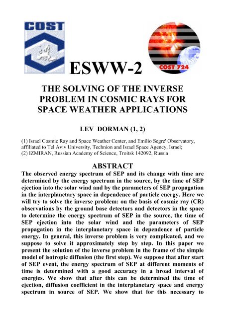
<strong>ESWW</strong>-2<br />
THE SOLVING OF THE INVERSE<br />
PROBLEM IN COSMIC RAYS FOR<br />
SPACE WEATHER APPLICATIONS<br />
LEV DORMAN (1, 2)<br />
(1) Israel Cosmic Ray and <strong>Space</strong> <strong>Weather</strong> Center, and Emilio Segre' Observatory,<br />
affiliated to Tel Aviv University, Technion and Israel <strong>Space</strong> Agency, Israel;<br />
(2) IZMIRAN, Russian Academy of Science, Troitsk 142092, Russia<br />
ABSTRACT<br />
The observed energy spectrum of SEP and its change with time are<br />
determined by the energy spectrum in the source, by the time of SEP<br />
ejection into the solar wind and by the parameters of SEP propagation<br />
in the interplanetary space in dependence of particle energy. Here we<br />
will try to solve the inverse problem: on the basis of cosmic ray (CR)<br />
observations by the ground base detectors and detectors in the space<br />
to determine the energy spectrum of SEP in the source, the time of<br />
SEP ejection into the solar wind and the parameters of SEP<br />
propagation in the interplanetary space in dependence of particle<br />
energy. In general, this inverse problem is very complicated, and we<br />
suppose to solve it approximately step by step. In this paper we<br />
present the solution of the inverse problem in the frame of the simple<br />
model of isotropic diffusion (the first step). We suppose that after start<br />
of SEP event, the energy spectrum of SEP at different moments of<br />
time is determined with a good accuracy in a broad interval of<br />
energies. We show that after this can be determined the time of<br />
ejection, diffusion coefficient in the interplanetary space and energy<br />
spectrum in source of SEP. We show that for this necessary to
determine energy spectrum of SEP on the Earth at least in three<br />
different moments of time.<br />
1. Observation data and inverse problems for isotropic<br />
diffusion, for anisotropic diffusion, and for kinetic description<br />
of solar CR propagation<br />
It is well known that Solar Energetic Particle (SEP) events in the beginning stage are very<br />
anisotropic, especially during great events as in February 1956, July 1959, August 1972,<br />
September-October 1989, July 2000, January 2005, and many others (Dorman, M1957, M1963a,b,<br />
M1978; Dorman and Miroshnichenko, M1968; Miroshnichenko, M2001). To determine on the<br />
basis of experimental data the properties of the SEP source and parameters of propagation, i.e. to<br />
solve the inverse problem, is very difficult, and it needs data from many CR stations. By the<br />
procedure developed in Dorman and Zukerman (2003), Dorman, Pustil’nik, Sternlieb, and<br />
Zukerman, 2005; see review in Chapter 3 in Dorman, M2004), for each CR station the starting<br />
moment of SEP event can be automatically determined and then for different moments of time by<br />
the method of coupling functions to determine the energy spectrum of SEP out of the atmosphere<br />
above the individual CR station. As result we may obtain the planetary distribution of SEP intensity<br />
out of the atmosphere and then by taking into account the influence of geomagnetic field on<br />
particles trajectories – the SEP angle distribution out of the Earth’s magnetosphere. By this way by<br />
using of the planetary net of CR stations with on-line registration in real time scale can be organized<br />
the continue on-line monitoring of great ground observed SEP events (Dorman, Pustil’nik, Sternlieb<br />
et al., 2004; Mavromichalaki, Yanke, Dorman et al., 2004).<br />
In this paper we practically base on the two well established facts:<br />
1) the time of particle acceleration on the Sun and injection into solar wind is very short<br />
in comparison with time of propagation, so it can be considered as delta-function<br />
from time;<br />
2) the very anisotropic distribution of SEP with developing of the event in time after few<br />
scattering of energetic particles became near isotropic (well known examples of<br />
February 1956, September 1989 and many others).<br />
This paper is the first step for solution of inverse problem in the theory of solar CR propagation<br />
by using only one on-line detector on the ground for high energy particles and one on-line detector<br />
on satellite for small energies. Therefore we will base here on the simplest model of generation<br />
(delta function in time and in space) and on the simplest model of propagation (isotropic diffusion).<br />
The second step will be based on anisotropic diffusion, and the third – on kinetic description of SEP<br />
propagation in the interplanetary space.<br />
The observed energy spectrum of SEP and its change with time are determined by the energy<br />
spectrum in the source, by the time of SEP ejection into the solar wind and by the parameters of<br />
SEP propagation in the interplanetary space in dependence of particle energy. Here we will try to<br />
solve the inverse problem: on the basis of CR observations by the ground base detectors and<br />
detectors in the space to determine the energy spectrum of SEP in the source, the time of SEP<br />
ejection into the solar wind and the parameters of SEP propagation in the interplanetary space in<br />
dependence of particle energy. In general this inverse problem is very complicated, and we suppose<br />
to solve it approximately step by step. In this Section we present the solution of the inverse problem<br />
in the frame of the simple model of isotropic diffusion of solar CR (the first step). We suppose that<br />
after start of SEP event, the energy spectrum of SEP at different moments in time is determined<br />
with good accuracy in a broad interval of energies by the method of coupling functions (see in<br />
detail in Chapter 3 in Dorman, M2004). We show then that after this the time of ejection, diffusion<br />
coefficient in the interplanetary space and energy spectrum in source of SEP can be determined.<br />
This information, obtained on line on the basis of real-time scale data, may be useful also for<br />
radiation hazard forecasting.
2. The inverse problem for the case when diffusion coefficient<br />
depends only from particle rigidity<br />
In this case the solution of isotropic diffusion for the pointing instantaneous source described by<br />
function<br />
will be<br />
( R r,<br />
t)<br />
= N ( R)<br />
δ ( r)<br />
( t)<br />
Q , o δ<br />
(1)<br />
( R,<br />
r,<br />
t)<br />
= N ( R)<br />
× 2<br />
2π<br />
( κ ( R)<br />
t)<br />
N o<br />
[ ] ( ) ⎟ − ⎛ ⎞<br />
× ⎜ r<br />
2<br />
3 2<br />
1<br />
exp −<br />
1 , (2)<br />
⎜<br />
⎝ 4κ<br />
R t ⎠<br />
where r is the distance from the Sun, t is the time after ejection, No ( R)<br />
is the rigidity spectrum of<br />
total number of SEP at the source, and κ ( R)<br />
is the diffusion coefficient in the interplanetary space<br />
during SEP event. Let us suppose that at distance from the Sun r = r1<br />
= 1AU<br />
and at several<br />
moments of time ti ( i = 1,<br />
2,<br />
3,...)<br />
after SEP ejection into solar wind the observed rigidity spectrum<br />
out of the Earth’s atmosphere ( R r t ) N ( R)<br />
,<br />
N i i ≡ , 1 are determined in high energy range on the basis<br />
of ground CR measurements by neutron monitors and muon telescopes (by using method of<br />
coupling functions, spectrographic and global spectrographic methods, see review in Dorman,<br />
M2004)) as well as determined directly in low energy range on the basis of satellite CR<br />
measurements. Let us suppose also that the UT time of ejection T e as well as the diffusion<br />
coefficient κ ( R)<br />
and the SEP rigidity spectrum in source No ( R)<br />
are unknown. To solve the inverse<br />
problem, i.e. to determine these three unknown parameters, we need information on SEP rigidity<br />
spectrum Ni ( R)<br />
at least at three different moments of time T 1 , T 2 and T 3 (in UT). In this case for<br />
these three moments of time after SEP ejection into solar wind we obtain:<br />
t1 = T1<br />
−Te<br />
= x,<br />
t2<br />
= T2<br />
−Te<br />
= T2<br />
−T1<br />
+ x,<br />
t3<br />
= T3<br />
−Te<br />
= T3<br />
−T1<br />
+ x , (3)<br />
where T2 -T 1 and T3 -T 1 are known values and x = T1<br />
−Te<br />
is unknown value to be determined<br />
(because T e is unknown). From three equations for t 1,<br />
t 2 and t3<br />
of the type of Eq. 2 by taking into<br />
account Eq. 3 and dividing one equation on other for excluding unknown parameter No ( R)<br />
, we<br />
obtain two equations for determining unknown two parameters x and κ ( R)<br />
:<br />
x<br />
T2 T1<br />
4κ<br />
= −<br />
2 1 r<br />
( T −T<br />
+ x)<br />
x<br />
( R)<br />
⎧ N1(<br />
R)<br />
× ln⎨<br />
( x ( T2<br />
−T1<br />
+ x)<br />
)<br />
2 N ( R)<br />
− 3 2<br />
( T −T<br />
+ x)<br />
1<br />
T3 T1<br />
4κ<br />
= −<br />
3 1 r<br />
⎩<br />
2<br />
( R)<br />
⎧ N1(<br />
R)<br />
× ln⎨<br />
( x ( T3<br />
−T1<br />
+ x)<br />
)<br />
2 N ( R)<br />
− 3 2<br />
1<br />
⎩<br />
3<br />
⎫<br />
⎬ , (4)<br />
⎭<br />
⎫<br />
⎬ . (5)<br />
⎭<br />
To exclude unknown parameter κ ( R)<br />
let us divide Eq. 4 by Eq. 5; in this case we obtain equation<br />
for determining unknown e T T x − = 1 :<br />
[ ( T −T<br />
) Ψ − ( T −T<br />
) ] ( − Ψ)<br />
x = 1 , (6)<br />
2<br />
1<br />
3<br />
1
where<br />
3 2<br />
[ N1(<br />
R)<br />
( x ( T2<br />
−T1<br />
+ x)<br />
) N 2 ( R)<br />
]<br />
N ( R)<br />
( x ( T −T<br />
3 2<br />
+ x)<br />
) N ( R)<br />
ln<br />
Ψ = [ ( T3<br />
−T1<br />
) ( T2<br />
−T1<br />
) ] ×<br />
. (7)<br />
ln<br />
[ ]<br />
1<br />
Eq. 6 can be solved by the iteration method: as a first approximation, we can use<br />
x 1 = T1<br />
−Te<br />
≈ 500 sec which is the minimum time propagation of relativistic particles from the<br />
Sun to the Earth’s orbit. Then, by Eq. 7 we determine Ψ ( x1<br />
) and by Eq. 6 we determine the second<br />
approximation x 2 . To put x 2 in Eq. 7 we compute Ψ ( x2<br />
) , and then by Eq. 6 we determine the<br />
third approximation x 3 , and so on. After solving Eq. 6 and determining the time of ejection, we can<br />
compute very easily diffusion coefficient from Eq. 4 or Eq. 5:<br />
( T2<br />
−T1<br />
) 4x(<br />
T2<br />
−T1<br />
+ x)<br />
1(<br />
R)<br />
3 2<br />
( x ( T2<br />
−T1<br />
+ x)<br />
)<br />
( R)<br />
3<br />
1<br />
3<br />
( T3<br />
−T1<br />
) 4x(<br />
T3<br />
−T1<br />
+ x)<br />
1(<br />
R)<br />
3 2<br />
( x ( T3<br />
−T1<br />
+ x)<br />
)<br />
( R)<br />
2<br />
2<br />
r<br />
1<br />
r<br />
1<br />
κ ( R)<br />
= −<br />
= −<br />
. (8)<br />
⎧ N<br />
⎫ ⎧ N<br />
⎫<br />
ln⎨<br />
⎬ ln⎨<br />
⎬<br />
⎩ N 2<br />
⎭ ⎩ N3<br />
⎭<br />
After determining the time of ejection and diffusion coefficient, it is easy to determine the SEP<br />
source spectrum:<br />
N o<br />
( ) 1/<br />
2 ( ) ( ( ) ) 3/<br />
2 2<br />
R = 2 N R × κ R x expr<br />
/ ( 4κ<br />
( R)<br />
x)<br />
π<br />
1<br />
= 2π1/<br />
2 N2<br />
= 2π1/<br />
2 N3<br />
( 1 )<br />
3/<br />
2 2<br />
+ x exp(<br />
r1<br />
/ ( 4κ<br />
R T2<br />
−T1<br />
+ x ) )<br />
3/<br />
2 2<br />
+ x exp(<br />
r / ( 4κ<br />
R T −T<br />
+ x ) ) .<br />
( 9)<br />
( R)<br />
× ( κ(<br />
R)(<br />
T −T<br />
) ) ( )( )<br />
2<br />
( R)<br />
× ( κ(<br />
R)(<br />
T −T<br />
) ) ( )( )<br />
3<br />
1<br />
1<br />
3. The inverse problem for the case when diffusion coefficient<br />
depends from the particle rigidity and the distance to the Sun<br />
Let us suppose, according to Parker (M1963), that the diffusion coefficient<br />
( ) ( ) ( ) β<br />
R , r κ R × r r<br />
In this case the solution of diffusion equation will be<br />
N<br />
( R,<br />
r,<br />
t)<br />
=<br />
N o<br />
1<br />
κ = 1 1 . (10)<br />
( ) ( ) ( ( ) ) ( )<br />
( ) ( ) ( ) ( ( ) ) ( ) ( ) ⎟⎟<br />
3β<br />
2−β<br />
−3<br />
2−β<br />
×<br />
⎛ β 2−β<br />
R r<br />
⎞<br />
1 κ1<br />
R t<br />
×<br />
⎜ r1<br />
r<br />
exp<br />
⎜<br />
−<br />
4+<br />
β 2−β<br />
2<br />
2 − β<br />
Γ 3 2 − β<br />
2 − β κ R t<br />
3<br />
⎝<br />
1<br />
1<br />
⎠<br />
, (11)<br />
where t is the time after SEP ejection into solar wind. So now we have four unknown parameters:<br />
time of SEP ejection into solar wind T e , β , κ 1(<br />
R)<br />
, and No ( R)<br />
. Let us assume that according to<br />
ground and satellite measurements at the distance r = r1<br />
= 1 AU from the Sun we know<br />
N1 ( R)<br />
, N2(<br />
R)<br />
, N3(<br />
R)<br />
, N4(<br />
R)<br />
at UT times T 1, T2<br />
, T 3 , T4<br />
. In this case<br />
For each N ( R r r , T )<br />
i<br />
t1 = T1<br />
−Te<br />
= x,<br />
t2<br />
= T2<br />
−T1<br />
+ x,<br />
t3<br />
= T3<br />
−T1<br />
+ x,<br />
t4<br />
= T4<br />
−T1<br />
+ x , (2.34.12)<br />
, = 1 i we obtain from Eq. 2.34.11 and Eq. 2.34.12:
Ni<br />
( R,<br />
r = r , T )<br />
( ) ( ) ( ( )( ) ) ( )<br />
( ) ( ) ( ) 3β<br />
2−<br />
β<br />
−3<br />
2−<br />
β<br />
R × r1<br />
κ1<br />
R Ti<br />
− T1<br />
+ x<br />
4+<br />
β 2−<br />
β<br />
2 − β<br />
Γ(<br />
3 ( 2 − β ) )<br />
( )<br />
( )( ) ,<br />
2 −2<br />
r1<br />
2 − β ⎞<br />
R T − T + x<br />
1 exp<br />
⎟<br />
1 1<br />
⎟<br />
No<br />
⎛<br />
⎜<br />
i =<br />
× −<br />
⎜<br />
⎝<br />
κ i ⎠<br />
where i = 1, 2, 3, and 4. To determine x let us step by step exclude unknown parameters No ( R)<br />
,<br />
κ 1(<br />
R)<br />
, and then β . In the first we exclude No ( R)<br />
by forming from four Eq. 13 for different i three<br />
equations for ratios<br />
−3<br />
( 2−<br />
β )<br />
2<br />
N1(<br />
R,<br />
r = r1,<br />
T1<br />
) ⎛ x ⎞<br />
⎛<br />
exp⎜<br />
r<br />
=<br />
× −<br />
1<br />
( , , ) ⎜<br />
⎟<br />
N =<br />
⎜ 2<br />
i R r r1<br />
Ti<br />
⎝ Ti<br />
− T1<br />
+ x ⎠<br />
⎝ 2 − β κ1<br />
( ) ( R)<br />
⎛ 1 1 ⎞⎞<br />
⎟<br />
⎜ −<br />
⎟ ,<br />
⎝ x T ⎟<br />
i − T1<br />
+ x ⎠⎠<br />
where i = 2, 3, and 4. To exclude κ 1(<br />
R)<br />
let us take logarithm from both parts of Eq. 2.34.14 and<br />
then divide one equation on another; as result we obtain following two equations:<br />
ln<br />
ln<br />
ln<br />
ln<br />
( N1<br />
N 2 ) + ( 3 ( 2 − β ) ) ln(<br />
x ( T2<br />
−T1<br />
+ x)<br />
)<br />
( N N ) + ( 3 ( 2 − β ) ) ln(<br />
x ( T −T<br />
+ x)<br />
)<br />
1<br />
3<br />
( N1<br />
N 2 ) + ( 3 ( 2 − β ) ) ln(<br />
x ( T2<br />
−T1<br />
+ x)<br />
)<br />
( N N ) + ( 3 ( 2 − β ) ) ln(<br />
x ( T −T<br />
+ x)<br />
)<br />
1<br />
4<br />
3<br />
4<br />
1<br />
1<br />
=<br />
=<br />
( 1 x)<br />
− ( 1 ( T2<br />
−T1<br />
+ x)<br />
)<br />
( 1 x)<br />
− ( 1 ( T −T<br />
+ x)<br />
)<br />
3<br />
( 1 x)<br />
− ( 1 ( T2<br />
−T1<br />
+ x)<br />
)<br />
( 1 x)<br />
− ( 1 ( T −T<br />
+ x)<br />
)<br />
4<br />
1<br />
1<br />
(13)<br />
(14)<br />
, (15)<br />
. (16)<br />
After excluding from Eq. 15 and Eq. 16 unknown parameter β , we obtain equation for determining<br />
x:<br />
where<br />
2<br />
( a a − a a ) + xd(<br />
a b + b a − a b − b a ) + d ( b b − b b ) = 0<br />
2<br />
x 1 2 3 4 1 2 1 2 3 4 3 4 1 2 3 4 , (17)<br />
( T −T<br />
)( T −T<br />
)( T T ),<br />
d = 2 1 3 1 4 − 1<br />
(18)<br />
( T −T<br />
)( T −T<br />
) ( N N ) − ( T −T<br />
)( T T ) ln(<br />
N N ),<br />
a1 = 2 1 4 1 ln 1 3 3 1 4 − 1 1 2 (19)<br />
a 2 = ( T3<br />
−T1<br />
)( T4<br />
−T1<br />
) ln( x ( T2<br />
−T1<br />
+ x)<br />
) − ( T2<br />
−T1<br />
)( T3<br />
−T1<br />
) ln(<br />
x ( T4<br />
−T1<br />
+ x)<br />
), (20)<br />
( T −T<br />
)( T −T<br />
) ( N N ) − ( T −T<br />
)( T T ) ln(<br />
N N ),<br />
a3 = 2 1 3 1 ln 1 4 3 1 4 − 1 1 2 (21)<br />
a 4 = ( T3<br />
−T1<br />
)( T4<br />
−T1<br />
) ln( x ( T2<br />
−T1<br />
+ x)<br />
) − ( T2<br />
−T1<br />
)( T4<br />
−T1<br />
) ln(<br />
x ( T3<br />
−T1<br />
+ x)<br />
), (22)<br />
b 1 = ln( N1<br />
N3<br />
) − ln(<br />
N1<br />
N 2 ) , b2<br />
= ln(<br />
x ( T2<br />
−T1<br />
+ x)<br />
) − ln(<br />
x ( T4<br />
−T1<br />
+ x)<br />
), (23)<br />
b 3 = ln( N1<br />
N 4 ) − ln(<br />
N1<br />
N 2 ) , b4<br />
= ln(<br />
x ( T2<br />
−T1<br />
+ x)<br />
) − ln(<br />
x ( T3<br />
−T1<br />
+ x)<br />
). (24)<br />
As it can be seen from Eq. 20 and Eq. 22-24, coefficients a 2 , a4<br />
, b2<br />
, b4<br />
very weekly (as logarithm)<br />
depend from x. Therefore Eq. 17 we solve by iteration method, as above we solved Eq. 6: as a first<br />
approximation, we use 1 = 1 − e ≈ 500 sec<br />
T T x (which is the minimum time propagation of
elativistic particles from the Sun to the Earth’s orbit). Then by Eq. 20 and Eq. 22-24 we determine<br />
a 2 ( x1<br />
) , a4<br />
( x1<br />
) , b2<br />
( x1<br />
) , b4<br />
( x1<br />
) and by Eq. 17 we determine the second approximation x 2 , and<br />
so on. After determining x, i.e. according Eq. 12 determining t 1 , t2<br />
, t3<br />
, t4<br />
, the final solutions for<br />
β , κ 1(<br />
R)<br />
, and N o ( R)<br />
can be found. Unknown parameter β in Eq. 10 we determine from Eq. 15<br />
and Eq. 16:<br />
−1<br />
⎡<br />
t ( )<br />
( ( ) ) 3 t2<br />
− t1<br />
⎤ ⎡<br />
t ( )<br />
2 3 ln<br />
ln(<br />
) ( ln(<br />
) ) 3 t2<br />
− t1<br />
⎤<br />
β = − ⎢ t2<br />
t1<br />
−<br />
t3<br />
t1<br />
⎥ × ⎢ N1<br />
N2<br />
− ln(<br />
N1<br />
N3<br />
) ⎥ . (25)<br />
⎣<br />
t2<br />
( t3<br />
− t1)<br />
⎦ ⎣<br />
t2<br />
( t3<br />
− t1)<br />
⎦<br />
Then we determine unknown parameter ( R)<br />
κ<br />
1<br />
2 −1<br />
−1<br />
r ( )<br />
( ) 1 t1<br />
− t<br />
R =<br />
2<br />
κ 1 in Eq. 10 from Eq. 14:<br />
−1<br />
−1<br />
( t − t )<br />
2<br />
r<br />
=<br />
1 1 3<br />
2<br />
3( 2 − β ) ln(<br />
t2<br />
t1)<br />
− ( 2 − β ) ln(<br />
N1<br />
N2<br />
) 3<br />
3 1<br />
1 3<br />
( ) ( ) ( ) ( ) .<br />
2<br />
2 − β ln t t − 2 − β ln N N<br />
After determining parameters β and κ ( R)<br />
we can determine the last parameter ( R)<br />
13:<br />
No<br />
( ) ( ) ( ) ( ) 4+<br />
β 2−<br />
β<br />
−3β<br />
( ( ) ) ( 2−<br />
β )<br />
R = N 2 − β<br />
Γ 3 2 − β r ( κ ( R)<br />
t )<br />
i<br />
1<br />
1<br />
1<br />
i<br />
3<br />
( )<br />
⎛<br />
2−<br />
β<br />
× exp⎜<br />
⎜<br />
⎝<br />
(26)<br />
N o from Eq.<br />
2<br />
r<br />
( ) ( ) ⎟ ⎟ 1<br />
2<br />
2 − β κ R t<br />
1<br />
⎞<br />
(27)<br />
i ⎠<br />
where index i = 1, 2 or 3.<br />
Above we show that for some simple model of SEP propagation is possible to solve inverse<br />
problem based on ground and satellite measurements at the beginning of the event. Obtained results<br />
we used in the method of great radiation hazard forecasting based on on-line CR one-minute ground<br />
and satellite data (Dorman, Iucci, Murat et al., 2005).<br />
Let us note that described solutions of inverse problem may be partly useful for solving more<br />
complicated inverse problems in case of SEP propagation described by anisotropic diffusion and by<br />
kinetic equation.<br />
ACKNOWLEDGEMENTS<br />
This research was partly supported by COST-724.<br />
REFERENCES<br />
Dorman L.I., Cosmic Ray Variations. Gostekhteorizdat, Moscow, M1957 (in Russian). English<br />
translation: US Department of Defense, Ohio Air-Force Base, M1958.<br />
Dorman L.I., Geophysical and Astrophysical Aspects of Cosmic Rays. North-Holland, Amsterdam,<br />
in series ‘Progress in Physics of Cosmic Ray and Elementary Particles’, ed. J.G. Wilson and<br />
S.A. Wouthuysen, Vol. 7, pp. 1-324, M1963a.<br />
Dorman L.I., Cosmic Ray Variations and <strong>Space</strong> Research. Nauka, Moscow, M1963b (in Russian).<br />
Dorman L.I., Cosmic Rays of Solar Origin, VINITI, Moscow (in series ‘Summary of Science’,<br />
<strong>Space</strong> Investigations, Vol.12), M1978 (in Russian).<br />
Dorman L.I., Cosmic Rays in the Earth’s Atmosphere and Underground, Kluwer Academic<br />
Publishers, Dordrecht/Boston/London, M2004.<br />
Dorman L.I. and L.I. Miroshnichenko, Solar Cosmic Rays, Physmatgiz, Moscow, M1968 (in<br />
Russian). English translation: NASA, Washington, DC, M1976.
Dorman L.I., L.A. Pustil’nik, A. Sternlieb, and I.G. Zukerman ‘Forecasting of Radiation Hazard: 1.<br />
Alerts on Great FEP Events Beginning; Probabilities of False and Missed Alerts; on-Line<br />
Determination of Solar Energetic Particle Spectrum by using Spectrographic Method’, Adv.<br />
<strong>Space</strong> Res., 35, (2005), in press.<br />
Dorman L.I., L.A. Pustil’nik, A. Sternlieb, I.G. Zukerman, A.V. Belov, E.A. Eroshenko, V.G.<br />
Yanke, H. Maromichalaki, C. Sarlanis, G. Souvatzoglou, S. Tatsis, N. Iucci, G. Villoresi, Yu.<br />
Fedorov, B.A. Shakhov, and M. Murat ‘Monitoring and Forecasting of Great Solar Proton<br />
Evnts Using the Neutron Monitor Network in Real Time’, IEEE Transactions on Plasma<br />
Science, 0093-3813, pp. 1-11 (2004).<br />
Dorman L. and I. Zukerman ‘Initial Concept for Forecasting the Flux and Energy Spectrum of<br />
Energetic Particles Using Ground-Level Cosmic Ray Observations’, Adv. <strong>Space</strong> Res., 31, No.<br />
4, 925-932 (2003).<br />
Mavromichalaki H., V. Yanke, L. Dorman, N. Iucci, A. Chilingaryan, and O. Kryakunova,<br />
‘Neutron Monitor Network in Real Time and <strong>Space</strong> <strong>Weather</strong>’, Effects of <strong>Space</strong> <strong>Weather</strong> on<br />
Technology Infrastructure, ed. by I.A. Daglis, NATO Science Series II, Mathematics, Physics<br />
and Chemistry, 176, Kluwer Academic Publishers, Dordrecht, 301-317 (2004)<br />
Miroshnichenko L.I., Solar Cosmic Rays, Kluwer Ac. Publishers, Dordrecht/Boston/London,<br />
M2001.<br />
Parker E.N., Interplanetary Dynamical Processes, John Wiley and Suns, New York-London,<br />
M1963. In Russian (ed. L.I. Dorman; transl. L.I. Miroshnichenko): Inostrannaja Literatura,<br />
Moscow, M1965.