Ionospheric Scintillation Monitoring - ESA Space Weather Web Server
Ionospheric Scintillation Monitoring - ESA Space Weather Web Server
Ionospheric Scintillation Monitoring - ESA Space Weather Web Server

Create successful ePaper yourself
Turn your PDF publications into a flip-book with our unique Google optimized e-Paper software.
NOTTINGHAM<br />
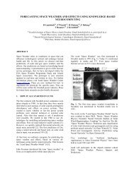
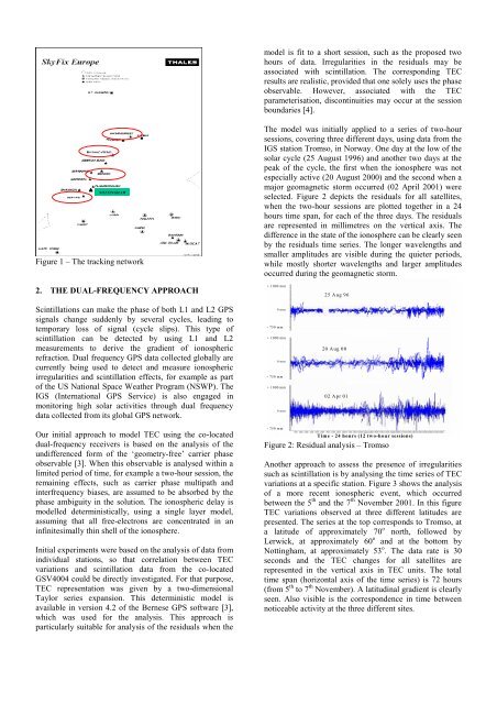
Figure 1 – The tracking network<br />
2. THE DUAL-FREQUENCY APPROACH<br />
<strong>Scintillation</strong>s can make the phase of both L1 and L2 GPS<br />
signals change suddenly by several cycles, leading to<br />
temporary loss of signal (cycle slips). This type of<br />
scintillation can be detected by using L1 and L2<br />
measurements to derive the gradient of ionospheric<br />
refraction. Dual frequency GPS data collected globally are<br />
currently being used to detect and measure ionospheric<br />
irregularities and scintillation effects, for example as part<br />
of the US National <strong>Space</strong> <strong>Weather</strong> Program (NSWP). The<br />
IGS (International GPS Service) is also engaged in<br />
monitoring high solar activities through dual frequency<br />
data collected from its global GPS network.<br />
Our initial approach to model TEC using the co-located<br />
dual-frequency receivers is based on the analysis of the<br />
undifferenced form of the ‘geometry-free’ carrier phase<br />
observable [3]. When this observable is analysed within a<br />
limited period of time, for example a two-hour session, the<br />
remaining effects, such as carrier phase multipath and<br />
interfrequency biases, are assumed to be absorbed by the<br />
phase ambiguity in the solution. The ionospheric delay is<br />
modelled deterministically, using a single layer model,<br />
assuming that all free-electrons are concentrated in an<br />
infinitesimally thin shell of the ionosphere.<br />
Initial experiments were based on the analysis of data from<br />
individual stations, so that correlation between TEC<br />
variations and scintillation data from the co-located<br />
GSV4004 could be directly investigated. For that purpose,<br />
TEC representation was given by a two-dimensional<br />
Taylor series expansion. This deterministic model is<br />
available in version 4.2 of the Bernese GPS software [3],<br />
which was used for the analysis. This approach is<br />
particularly suitable for analysis of the residuals when the<br />
model is fit to a short session, such as the proposed two<br />
hours of data. Irregularities in the residuals may be<br />
associated with scintillation. The corresponding TEC<br />
results are realistic, provided that one solely uses the phase<br />
observable. However, associated with the TEC<br />
parameterisation, discontinuities may occur at the session<br />
boundaries [4].<br />
The model was initially applied to a series of two-hour<br />
sessions, covering three different days, using data from the<br />
IGS station Tromso, in Norway. One day at the low of the<br />
solar cycle (25 August 1996) and another two days at the<br />
peak of the cycle, the first when the ionosphere was not<br />
especially active (20 August 2000) and the second when a<br />
major geomagnetic storm occurred (02 April 2001) were<br />
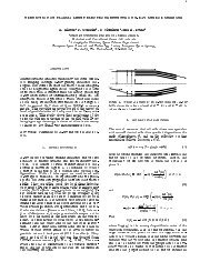
selected. Figure 2 depicts the residuals for all satellites,<br />
when the two-hour sessions are plotted together in a 24<br />
hours time span, for each of the three days. The residuals<br />
are represented in millimetres on the vertical axis. The<br />
difference in the state of the ionosphere can be clearly seen<br />
by the residuals time series. The longer wavelengths and<br />
smaller amplitudes are visible during the quieter periods,<br />
while mostly shorter wavelengths and larger amplitudes<br />
occurred during the geomagnetic storm.<br />
+ 1000 mm<br />
0 mm<br />
- 750 mm<br />
+ 1000 mm<br />
0 mm<br />
- 750 mm<br />
+ 1000 mm<br />
0 mm<br />
- 750 mm<br />
25 Aug 96<br />
20 Aug 00<br />
02 Apr 01<br />
Time - 24 hours (12 two-hour sessions)<br />
Figure 2: Residual analysis – Tromso<br />
Another approach to assess the presence of irregularities<br />
such as scintillation is by analysing the time series of TEC<br />
variations at a specific station. Figure 3 shows the analysis<br />
of a more recent ionospheric event, which occurred<br />
between the 5 th and the 7 th November 2001. In this figure<br />
TEC variations observed at three different latitudes are<br />
presented. The series at the top corresponds to Tromso, at<br />
a latitude of approximately 70 o north, followed by<br />
Lerwick, at approximately 60 o and at the bottom by<br />
Nottingham, at approximately 53 o . The data rate is 30<br />
seconds and the TEC changes for all satellites are<br />
represented in the vertical axis in TEC units. The total<br />
time span (horizontal axis of the time series) is 72 hours<br />
(from 5 th to 7 th November). A latitudinal gradient is clearly<br />
seen. Also visible is the correspondence in time between<br />
noticeable activity at the three different sites.