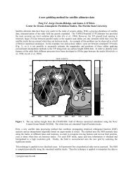
A numerical model of coastal upwelling. - Center for Ocean ...
A numerical model of coastal upwelling. - Center for Ocean ...
A numerical model of coastal upwelling. - Center for Ocean ...

Create successful ePaper yourself
Turn your PDF publications into a flip-book with our unique Google optimized e-Paper software.
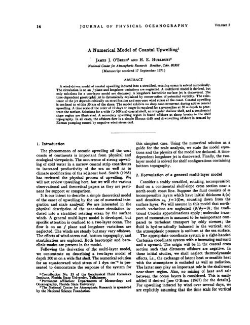
14<br />
1. Introduction<br />
)OURNAL OF PHYSICAL OCEANOGRAPHY<br />
A Numerical Model <strong>of</strong> Coastal Upwellingl<br />
JAKES J. O'BRIEN' AND H. E. HURLBURT'<br />
National CmIer <strong>for</strong> Almospheric Research BOIJdv, Clio. 8OJQZ<br />
(Manuscript received 17 September 1971)<br />
ABSTRACT<br />
A wind-driven <strong>model</strong> <strong>of</strong> <strong>coastal</strong> <strong>upwelling</strong> induced into a stratified, rotating ocean is, solved <strong>numerical</strong>ly.<br />
The circulation is on an fplane and longshore variations are neglected. A multilevel <strong>model</strong> is derived, but<br />
only solutions <strong>for</strong> a two-layer <strong>model</strong> are discussed. A longshore baroclinic surface jet is discovered. The<br />
time-dependent geostrophic jet is dynamically explained by conservation <strong>of</strong> potential vorticity. The existtence<br />
<strong>of</strong> the jet depends critically on stratification and non-zero wind stress at the coast. Coastal <strong>upwelling</strong><br />
is confined to within 30 km <strong>of</strong> the shore. The <strong>model</strong> exhibits no deep countercurrent during active <strong>coastal</strong><br />
<strong>upwelling</strong>. A time scale <strong>of</strong> the order <strong>of</strong> 10 days or longer is required <strong>for</strong> a pycnocline at 50 m depth to penetrate<br />
the surface. Solutions <strong>for</strong> a \\ide (>300 km).<strong>coastal</strong> shelf, an irregular shallow shelf, and a continental<br />
slope region are illustrated. A secondary <strong>upwelling</strong> region is found <strong>of</strong>fshore at sharp breaks in the shelf<br />
~aphy. In all cases, the <strong>of</strong>fshore flow is a simple Ekman drift and downwelling <strong>of</strong>fshore is created by<br />
Ekman pumping caused by negative wind-stress curl.<br />
The phenomenon <strong>of</strong> oceanic <strong>upwelling</strong> <strong>of</strong>f the west<br />
coasts <strong>of</strong> continents is important from physical and<br />
ecological viewpoints. The occurrence <strong>of</strong> strong <strong>upwelling</strong><br />
<strong>of</strong> cold water in a narrow <strong>coastal</strong> strip contributes<br />
to increased productivity <strong>of</strong> the sea as well as to<br />
climate modification <strong>of</strong> the adjacent land. Smith (1968)<br />
has reviewed the physical process <strong>of</strong> <strong>upwelling</strong>. We<br />
will not review <strong>upwelling</strong> here, but we will cite various<br />
observational and theoretical papers as they are pertinent<br />
<strong>for</strong> support or comparison.<br />
It is our intent to describe a simple theoretical <strong>model</strong><br />
<strong>of</strong> the onset <strong>of</strong> <strong>upwelling</strong> by the use <strong>of</strong> <strong>numerical</strong>integration<br />
and scale analysit. We are interested in the<br />
physical description <strong>of</strong> the near-shore circulation induced<br />
into a stratified rotating ocean by the surface<br />
winds. A general multi-layer <strong>model</strong> is developed, but<br />
specific attention is confined to a two-layer ocean. The<br />
Bow is on an f plane and longshore variations are<br />
neglected. The winds are steady but may vary <strong>of</strong>fshore.<br />
The effects <strong>of</strong> wind-stress curl, bottom topography, and<br />
stratification are explored. Both barotropic and baroclinic<br />
modes are present in the <strong>model</strong>.<br />
Following the derivation <strong>of</strong> -t4e multi-layer <strong>model</strong>,<br />
we concentrate on describing a two-layer <strong>model</strong> <strong>of</strong><br />
depth 200 m on a wide Bat shelf. The <strong>numerical</strong> solution<br />
<strong>for</strong> an equatorward wind stress <strong>of</strong> 1 dyn an~ is presented<br />
to demonstrate the response <strong>of</strong> the system <strong>for</strong><br />
-<br />
1 Contn"bution No. SS <strong>of</strong> the Geophysi(:al Fluid Dynamics<br />
Institute, Florida State University, T.~assee.<br />
t Pennanent affiliation: Departments <strong>of</strong> Meteorology and<br />
<strong>Ocean</strong>ography, Florida State University.<br />
a The National <strong>Center</strong> <strong>for</strong> Atmospheric Research is sponsored<br />
by the National Science Foundation.<br />
VOLUME 2<br />
this simplest case. Using the <strong>numerical</strong> solution as a<br />
guide <strong>for</strong> the scale analysis, we scale the <strong>model</strong> equations<br />
and the physics <strong>of</strong> the <strong>model</strong>aie deduced. A time-<br />
dependent longshore jet is discovered. Finally, the twolayer<br />
<strong>model</strong> is solved <strong>for</strong> shelf configurations containing<br />
bottom topography.<br />
2. Formulation <strong>of</strong> a general multi-layer <strong>model</strong><br />
Consider a stably stratified, rotating, incompressible<br />
fluid on a continental shelf-slope crbSS section near a<br />
north-south coast line. Suppose the fluid consists <strong>of</strong> m<br />
incompressible layers which have initial thickness 1I;(x)<br />
and densities Ph j = 1 (l)m, counting down from the<br />
surface layer. We will assume in this <strong>model</strong> that northsouth<br />
variations are neglected (a/a,=O); the traditional<br />
Coriolis approximations apply; molecular transport<br />
<strong>of</strong> momentum is assumed to be unimportant compared<br />
to turbulent transport by eddy stresses; the<br />
fluid is hydrostatically balanced in the vertical; and<br />
the atmospheric pressure is uni<strong>for</strong>m at the sea surface.<br />
The appropriate {;oordinate system is a right-handed<br />
Cartesian coordinate system with x increasing eastward<br />
and s upward. The origin will be in the <strong>coastal</strong> cross<br />
section such that distances <strong>of</strong>fshore are negative. In<br />
these initial studies, we shall neglect thennodynamic<br />
effects, i.e., the exchange <strong>of</strong> latent heat or sensible heat<br />
with the atmosphere is excluded as well as radiation.<br />
The latter may play an important role in the shallowest<br />
near-shore region. Also, no mixing <strong>of</strong> heat and ,salt<br />
between the ocean layers is considered. This is easily<br />
added if desired [see O'Brien (1967) <strong>for</strong> the detailsJ.<br />
For <strong>upwelling</strong> induced by wind over several days, we<br />
are explicitly assuming that the time scale <strong>for</strong> vertical
JANUARY 1972<br />
J I<br />
mixing is much slower than that <strong>for</strong> vertical transport<br />
<strong>of</strong> fluid.<br />
We are particularly interested in the vertically averaged<br />
velocity within each layer and the vertical velocity<br />
at the interface <strong>of</strong> each layer. If the pertinent<br />
hydrodynamic equations <strong>of</strong> motion are integrated<br />
vertically over the depth <strong>of</strong> each layer and the vertically<br />
averaged horizontal velocity components I'i, 'OJ are<br />
assumed independent <strong>of</strong> depth within eaCh layer, we<br />
obtain<br />
aUi<br />
at<br />
aui '1'.<br />
+ur-+Pi- ~s+[(... .<br />
8:% i<br />
avi<br />
~<br />
at<br />
av;<br />
ax<br />
Bs<br />
'1', )/pilJ+A<br />
,.. B.<br />
--~(.,. -.,. )/ph;]+A<br />
I ;<br />
O'BRIEN AND H E HURLBURT<br />
a2Ui<br />
-,<br />
ax'<br />
a~;<br />
-, ar<br />
(1)<br />
(2)<br />
alii allJUi<br />
I -0, (3)<br />
at axwhere<br />
P; is the pressure integral <strong>for</strong> the layer and T r<br />
and TIJ are the stresses at the top and bottom <strong>of</strong> each<br />
layer. When j=l, ~r =Tf~+iTfY, where these components<br />
are the wind stresses at the sea surface. They will<br />
be specified as functions <strong>of</strong> x and t. The vertical velocity<br />
is implicit in (3) and may be obtained a posteriori from<br />
the h; and 11; fields. Both barotropic and baroclinic<br />
modes have been retained. The barotropic mode will<br />
be shown to be fundamentally important <strong>for</strong> the winddriven<br />
<strong>upwelling</strong> problem. It has been neglected by<br />
previous investigators.<br />
o. The pressure integrals<br />
From the hydrostatic assumption, it follows that the<br />
pressure p, at any point inSide ,a layer k is given by<br />
layer 1<br />
: layer 21<br />
1-1 ~.<br />
Pt,=P.4+ #1 PJthl+p.,[/=J ~I+D(x)-.],<br />
layer<br />
(-i)<br />
where m is the number <strong>of</strong> discrete layers, P A the uni<strong>for</strong>m<br />
atmospheric pressure, and D(x) the elevation <strong>of</strong><br />
the bottom above the reference level s=O. The influence<br />
<strong>of</strong> the torque <strong>of</strong> the atmospheric pressure<br />
gradient may be included if desired (e.g., Galt, 1971).<br />
The x derivatives <strong>of</strong> these pressures are<br />
apt "-1 ah; {<br />
-- y psg-:-+p<br />
-. all--i a<br />
j<br />
~ -+- .<br />
ax 1=1 ax ~ ax as<br />
(5)<br />
1$<br />
Integrating these over the appropriate layer, we find<br />
that<br />
1 12' at'.<br />
PJli= - -=-ds<br />
p. B a~<br />
h. ~l ani - { -. all-; a<br />
- I:; pJt-:-+h ~ -+- ~<br />
p. 1-1 a~ ~ ax ax<br />
(6)<br />
These values <strong>of</strong> P. are used in (1). Thus, <strong>for</strong> an appropriate<br />
specification <strong>of</strong> th~ wind stress, a functional<br />
<strong>for</strong>m <strong>of</strong> the interior stresses, and valid initial and<br />
boundary conditions, the <strong>for</strong>mal statement <strong>of</strong> the<br />
problem will be complete.<br />
The <strong>for</strong>m <strong>of</strong> P. can be simplified if either 1) the<br />
bottom layer (or layers) is at rest or 2) there is no<br />
bottom topography.<br />
b. Initial conditions and boundary conditions<br />
There are several allowable initial conditions. First,<br />
if the interface surfaces are horizontal, then the appropriate<br />
initial condition is Ui=lIi=O. If Pi does not<br />
vanish initially in any layer, the initial conditions may<br />
be Ui=O, flli=Pi, i.e., the layer is in geostrophic<br />
equilibrium.<br />
The velocity components vanish at the coast, i.e., at<br />
x=O. At x= - ~, the fluid velocity takes on its initial<br />
value. We anticipate specifying a wind-stress distribution<br />
that approaches zero far <strong>of</strong>fshore. In such a case,<br />
a radiational condition (Shapiro and O'Brien, 1970) or<br />
a viscous far field (Galt, 1971) may be used to close<br />
the solution at a computational outer boundary. We<br />
will demonstrate that the solution in the <strong>upwelling</strong><br />
zone is independent <strong>of</strong> the~<strong>for</strong>cing outside the <strong>upwelling</strong><br />
zone and thus apply far-field boundary conditions<br />
which cannot alter the solution near the coast in any<br />
significant way.<br />
c. The interior stresses<br />
The equations <strong>of</strong> motion (1)-(3) are coupled <strong>for</strong><br />
adjacent layers through the preSsure gradients P J and<br />
the interior stresses. To complete the statement <strong>of</strong> the<br />
problem, we must specify a functional <strong>for</strong>m <strong>of</strong> these<br />
stresses.<br />
The stresses must be continuous across the interfaces,<br />
i.e., "':.="'~1 and .,.:--.,.1;1' They act in opposition<br />
to one another on the interface and thus are<br />
balanced. We wish to choose a functional <strong>for</strong>m <strong>of</strong><br />
~j=.,.~+i.,.~ de~ndent upon the velocity q;=uJ+illj,<br />
but not dependent upon aq,Ios. The logical physical<br />
choice is a quadratic <strong>for</strong>m from a dimensional argument.<br />
To arrive at an appropriate <strong>for</strong>m, let us consider the<br />
energy equation.<br />
In general, <strong>for</strong> a continuously stratified system<br />
(A =0), one obtains an integral energy equation <strong>of</strong> the
16<br />
fOrD}<br />
aE<br />
JOURNAL OF PHYSICAL OCEANOGRAPHY<br />
1"<br />
-+VgoJat<br />
B<br />
a'f<br />
q.-ds=I,<br />
as<br />
(7)<br />
where E is the swn <strong>of</strong> the kinetic and potential energy<br />
densities and .J is an energy fiu..'t density. H we con.<br />
centrate our attention on the integral on the right (I),<br />
we can arrive at an integrated expression <strong>for</strong> I and<br />
eventually at a <strong>for</strong>m <strong>for</strong> 'C. The approach outlined<br />
below was suggested by Robert O. Reid (personal<br />
communication) <strong>for</strong> a somewhat different problem.<br />
Integrating I by parts, we obta.in<br />
I-[..'C]r-[q.'C]B'<br />
.r<br />
,1.<br />
If the velocity q or the stress ~ vanishes at the bottom,<br />
the second term vanishes. The first term is the rate <strong>of</strong><br />
supply <strong>of</strong> kinetic energy from the winds. The integral<br />
on the right represents collectively the rate <strong>of</strong> decrease<br />
<strong>of</strong> energy <strong>of</strong> the organized motion, i.e., the rate <strong>of</strong><br />
conversion to turbulence and ultimately to thermal<br />
energy. Moreover, from the second law <strong>of</strong> thermodynamics,<br />
we expect that the integrand<br />
aq<br />
>0.<br />
a.<br />
-<br />
e<br />
o<br />
-<br />
d<br />
z<br />
.<br />
aq<br />
az<br />
(8)<br />
(9)<br />
VOLUME 2<br />
3. The two-layer <strong>model</strong><br />
-<br />
We will explore the details <strong>of</strong> a two-layer <strong>model</strong>.<br />
Consider a two-layer fluid governed by the dynamics<br />
derived in the previous section. The equations are<br />
aU1 aU1<br />
-+u1--c-+g(h1+it+D).<br />
at ax<br />
- JVt+ ("aa_.,.,8)/(piIs) +A<br />
a~<br />
+.r ~+("s- - ,.,-)/ (plIv + A-,<br />
at a%<br />
,\...t<br />
Ot/l<br />
a.i<br />
attll<br />
-,<br />
ax'<br />
ah1<br />
,-<br />
ax<br />
8tu2<br />
- fts+("z8-orB8)/(p/I,)+A-,<br />
8r<br />
a"2
JANUARY 1972 J J<br />
O'BRIEN AND H. E. HURLBURT<br />
FIG. 1. Typical geometry <strong>for</strong> a two-layer <strong>model</strong> with a free surface and one interface.<br />
The bottom topography is D(z), and"l and"t are the thicknesses <strong>of</strong> each layer <strong>of</strong> density<br />
PI and Pt. The velocities are depth-averaged.<br />
For a nonlinear problem, we must resort to <strong>numerical</strong><br />
methods <strong>of</strong> solution. The techniques used are new and<br />
extremely efficient, and they are explained in the next<br />
section.<br />
Boundary conditions are required to close the problem.<br />
At the coast, Ui=Vl=Ut=v,=O and hl and h2 are<br />
determined from the continuity equation using a onesided<br />
finite difference. At x= - ~, all <strong>of</strong> the velocities<br />
vanish and hl and ht are independent <strong>of</strong> time. In the<br />
computer <strong>model</strong>, we should utilize a radiational condition<br />
or the method 9f characteristics at some large<br />
but finite distance from the coast. However, empirical<br />
experimentation demonstrated that infinite channel<br />
(no slip) boundary conditions at a considerable distance<br />
(~300 kIn) from the coast do n9t affect the solution in<br />
the <strong>coastal</strong> region. . . .<br />
500 ~a KAt 100<br />
0<br />
2<br />
N<br />
I~<br />
U<br />
f/)<br />
~<br />
0%<br />
~<br />
%-<br />
-I t-<br />
FIG. 2. Wmd stress components as a function <strong>of</strong> distance <strong>of</strong>fshore;<br />
, is 1 dyn cm-t Dear the coast; 7"'- is zero everywhere.<br />
-2<br />
It is practically impossible to obtain oceanographic<br />
estimates <strong>of</strong> -r(x,t) in <strong>upwelling</strong> regions. The data just<br />
do not exist. For this simple <strong>model</strong>, we choose a wind<br />
stress which is independent <strong>of</strong> time and space <strong>for</strong><br />
XE[O, -200 kIn] and drops <strong>of</strong>f rapidly in magnitude<br />
200 kIn <strong>of</strong>f the coast (Fig. 2).<br />
The parameters <strong>for</strong> the standard case are f = lij-4<br />
sec-i, g=lO' an sec-'!, D=O, T8s=O, p=l, A=lO' ant<br />
sec-i, g'=2, c=3Xlij-4. We have altered these <strong>for</strong><br />
various computer solutions. The importance <strong>of</strong> the<br />
parameter values will become clearer in the section on<br />
scale aD;alYSis.<br />
4. Semi-implicit method<br />
We have designed an extremely efficient <strong>numerical</strong><br />
scheme following the example <strong>of</strong> K wizak and Robert<br />
(1971). For the present one-dimensionallayered <strong>model</strong>,<br />
the scheme is sufficiently different from Kwizak and<br />
Robert that ,we shall present the technique in some<br />
detail.<br />
Since the equations contain external gravity waves<br />
as solutions (as :w-ell as internal gravity waves), the<br />
garden variety explicit finite-difference schemes require<br />
a tinle step At bounded above by 4%/(gB)t, where H is<br />
the total depth <strong>of</strong> the fluid. The fine resolution<br />
[4%=0(1 km)] and the deep fluid [H=0(1 kIn)],<br />
envisioned <strong>for</strong> realistic simulation <strong>of</strong> <strong>coastal</strong> <strong>upwelling</strong>,<br />
dictate a time-step < 1 min, whereas we anticipate<br />
integrating our <strong>model</strong> <strong>for</strong> days. Kwizak and Robert<br />
demonstrate that if we choose an implicit scheme <strong>for</strong><br />
the terms which govern the physics <strong>of</strong> the fastest<br />
moving waves, a much larger time step may be utilized.<br />
We elect to treat both the external gravity wave and
~<br />
18 JOURNAL OF PHYSICAL OCEANOGRAPHY<br />
VOLUllE2<br />
the internal gravity wave modes implicitly. If the<br />
pressure gradient terms in the momentum equations<br />
and the divergence term in the continuity equations<br />
are treated implicitly, then we may use a much larger<br />
time step, say on the order <strong>of</strong> 1 hr. Application <strong>of</strong> the<br />
following scheme resulted in a factor <strong>of</strong> 20 savings in<br />
computer time <strong>for</strong> the present problem on a CDC~;<br />
i.e., a 20-min integration time using an explicit finitedifference<br />
scheme is reduced to less than 1 min by<br />
using the semi-implicit method. Identical results were<br />
obtained using both methods.<br />
Consider the <strong>model</strong> equations in the <strong>for</strong>m<br />
~I+<br />
-2Al~+ilTl<br />
.- ~H1- 8II1J_l<br />
. 8s i<br />
~1-:-(h1 a + it+ D) .,.. 4tg'ailJe+l<br />
a~ 8s i<br />
-LIt (25)<br />
-2.6JU~+~1<br />
8 8il J -'<br />
~(iJ+it+D)-~t'-<br />
-Lt. (26)<br />
0..1 a<br />
-+t-:-(.h1+.h,+D)-Ul,<br />
at as<br />
ail 0..1 0..1 ail<br />
-+H~- -hI' -"I--Dt,<br />
at as as<br />
(19)<br />
(20)<br />
cJscJsiAi(H.+D)hI<br />
] -+-1<br />
hti-+l+<br />
Bsl<br />
ht J_I<br />
At(H.+D)-<br />
-<br />
ax<br />
8M, a a~l<br />
-+r(~l+ht+D) -g'-=<br />
at ~ a%<br />
Ut,<br />
(21)<br />
=2AJDI/'+itrl-<br />
-L.. (27)<br />
as I<br />
All spatial derivatives are replaced by second-order<br />
finite differences. The subscripts j and n imply <strong>for</strong> any<br />
ait<br />
-+(B.+D)-at<br />
8M,<br />
a~<br />
-11.'<br />
aus ail<br />
-~+D--DI,<br />
as as<br />
~<br />
as<br />
(22)<br />
scalar q that<br />
qj--q(-j~, 1IAI). (28)<br />
where B 1 is the mean depth <strong>of</strong> the upper layer and<br />
Bt+D the mean height <strong>of</strong> the interface between the<br />
two layers. No approximations have been made; Ul<br />
and U t are all the remaining tenns in the %-directed<br />
momentum equations. The linear part <strong>of</strong> the divergence<br />
term in the continuity equation is retained on the lefthand<br />
side. The primed quantities are defined by<br />
All <strong>of</strong> the right-hand side terms, defined now as L,<br />
(i= 1, 2, 3, 4), are "known" at any time level in the<br />
calculations. We wish to find (lIl,Ut,"I,"I)j_+l <strong>for</strong> all j<br />
at time level (11+ 1) AI. K wi.7.ak and Robert recommend<br />
elimination <strong>of</strong> the velocities and the solution <strong>of</strong> coupled<br />
Helmholtz equations <strong>for</strong> "1 and "1. Since we have<br />
homogeneous bQundary conditions <strong>for</strong> III and Ut, we<br />
elect to p-liminate "1 and "1 fIml the above and obtain<br />
it-il'+BI<br />
} .<br />
II-I,'+B,<br />
J ~1 l<br />
+(C-(J) [~<br />
tI~l-b[~ as' "<br />
]"'l<br />
{23)<br />
.<br />
It is important to ~ iliat Hi and Iit+D are constants.<br />
We will treat the left-hand side <strong>of</strong> (19)-(22)<br />
implicitly and the right-hand side explicitly. (We have<br />
-4, . 8,si I<br />
--V""l+NtJ-+ t+C[ ~ ] '" t<br />
-..<br />
8,si J<br />
(29)<br />
(.'to)<br />
also made the horizontal diffusive terDlS implicit using where 4=tH1~, b=t(Hs+D) ~, c-iH1~, and d<br />
the Crank-Nicholson method. This is not included and e are a linear combination <strong>of</strong> the L,. These equa-<br />
below to simplify the discussion.) The tendencies are<br />
evaluated over 2411 and the pressure gradient terms<br />
and the divergence terms are averaged between time<br />
levels (ft-1) 411 and (ft+ 1) 411.<br />
The time-differenced equations are<br />
tions are coupled one-dimensional, Helmholtz equations<br />
in the unknowns "1-+1 and fIt-+1 lor all space<br />
points j. When the spatial derivatives are replaced by<br />
standard second-order finite differences, the resulting<br />
algebraic equations are tridiagonal and are easily solved<br />
by the special "up-down" variant <strong>of</strong> Gaussian elimination.<br />
In practice, we solve (29) and (30) iteratively by<br />
.~.+<br />
solving (30) <strong>for</strong> "iJ'-+l using "up-down" and ~en (29)<br />
<strong>for</strong> flti-+l. Only a few scans are needed <strong>for</strong> convergence.<br />
The )'-directed momentum equations are solved using<br />
-2AIU~+-rl<br />
4l~(hl+il+D)<br />
8~<br />
]_l<br />
-Lit<br />
I<br />
(24)<br />
well known techniques-leap-frog <strong>for</strong> time differences,<br />
a quadratic-averaging method known as Scheme F from<br />
Grammeitvedt (1969) <strong>for</strong> the advective terms, Crank-<br />
Nicholson <strong>for</strong> the diffusive terms, and centered-in-time
~<br />
JANUARY 1972<br />
Coriolis terms. We believe it unnecessary to repeat<br />
these well-known finite-difIerence schemes here.<br />
5. Flat shelf case<br />
A simple flat shelf case is used to e.xplore the basic<br />
physics <strong>of</strong> our modd <strong>of</strong> the onset <strong>of</strong> <strong>upwelling</strong>. This<br />
standard <strong>model</strong> is integrated <strong>numerical</strong>ly until hi approaches<br />
zero near the wall. The solutions are shown<br />
in Figs. 3-10. The fluid is initially at rest with hi = 50 m,<br />
h, = 150 m <strong>for</strong> all x.<br />
In Fig. 3, the height anomaly <strong>of</strong> the interface and<br />
free surface are shown after 4 days. Near the shore in<br />
a width <strong>of</strong> 20 km or so, the interface height anomaly<br />
is order 10 m. The free surface anomaly is order - 20<br />
cm. Offshore, where .,.8 approaches zero, a negative<br />
height anomaly is calculated. We shall refer to positive<br />
height anomalies as <strong>upwelling</strong> and negative as downwelling.<br />
We shall demonstrate that the downwelling is<br />
simple Ekman pumping which occurs when curl ~ 8 is<br />
,<br />
J<br />
J. O'BRIEN AND H. E HURLBURT<br />
50<br />
.5<br />
~G<br />
~cn 0:<br />
50~<br />
~~<br />
20~<br />
t5 Zto<br />
E-o<br />
5:I:<br />
02<br />
-5t&1<br />
:I:<br />
-to<br />
-t5<br />
~O 200- KM tOO D -20<br />
FIG. 3. Interface height anomaly after 4 days as a function <strong>of</strong> %.<br />
Upwelling is indicated by positive height anomaly near the shore.<br />
Downwelling is found centered at 210 kID. The dashed line is the<br />
free surface anomaly. ~<br />
~<br />
IS<br />
.0<br />
S<br />
~<br />
~<br />
20<br />
15<br />
-20<br />
5OC 200 KM 100<br />
0<br />
10<br />
5<br />
0<br />
-5<br />
'1'<br />
19<br />
FIG. 5. Interface height anomaly after 10 days. The interface<br />
bas almost surfaced near the shore. The downwelling is centered<br />
near 210 km. The dashed line is the free surface anomaly.<br />
-100<br />
~O 200 KM tOO<br />
~<br />
I' aUtaJ<br />
-I' f/)<br />
"-<br />
-21 :s<br />
-,~ U<br />
~O ~<br />
-so >-<br />
E-<br />
~~ U 0<br />
-7' ~<br />
~<br />
-Be ><br />
FIG. 6. Velocity pr<strong>of</strong>iles as a function <strong>of</strong> s afw 10 days. Dashed<br />
lines are lower layer velocity components. A strong surface jet<br />
occurs near s=O. The longshore velocities are barotropic between<br />
50-150 kin.<br />
~O 200 KM 100 0 .<br />
\<br />
-~<br />
10<br />
9<br />
8<br />
rU1<br />
>ct;<br />
60<br />
5Z -<br />
rn<br />
~<br />
~<br />
~<br />
ze--<br />
:I:<br />
to)<br />
&3<br />
:I:<br />
.r:1 2<br />
.-<br />
3f-o<br />
2<br />
FIG. 7. Contours <strong>of</strong> fll as a function <strong>of</strong> time and ~ The<br />
inertial oscillations are visible. The minimum #1 is O( -3 CD!<br />
sec-1). The inertial oscillations decay in time in the <strong>for</strong>ced region.<br />
The oountdur interval is 1 cm sec-1.
~<br />
20<br />
JOURNAL OF PHYSICAL OCEANOGRAPHY<br />
~<br />
e<br />
VOLUMB2<br />
40<br />
cn<br />
~~<br />
5GCaJ<br />
Z5~<br />
202<br />
15 Z-<br />
10 E-<br />
5:1:<br />
0,9<br />
-5CaJ<br />
:I:<br />
-II<br />
-15<br />
- 200 KAt I" . -21<br />
FIG. 10. Interface ~t anomaly <strong>for</strong> each day as a function <strong>of</strong> ~.<br />
After 10 days, ..- 2 m at the w.n aDd 6Sm near 210 km.<br />
negative. The dynamics <strong>of</strong> the <strong>upwelling</strong> at the wall<br />
the height anomaly is alm~t 50 ro, i.e., hi is approaching<br />
zero. The downwelling OCCUR 200 km <strong>of</strong>fshore.<br />
The free surface anomaly is order -50 an. It is im-<br />
are more complicated.<br />
In Fig. 4, the four velocity components are shown<br />
after 4 days as a function <strong>of</strong> space. The upper layer<br />
Bow is <strong>of</strong>fshore (111
i ;. JANUARY 1972<br />
j. j. O'BRIEN ANP H E HURLBURT<br />
21<br />
tive, downwdling occurs through Ekman pun1ping.<br />
Except <strong>for</strong> the presence <strong>of</strong> the baroclinic jet and the<br />
narrowness <strong>of</strong> the <strong>upwelling</strong> region, this description is<br />
s [ HSOUs - au, a<br />
RsAs ~ at +Fr-
~<br />
22<br />
JOURNAL OF PHYSICAL OCEANOGRAPHY V~UME2<br />
the multiple balance. The horizontal friction tenn is hI/hIe> 1. There<strong>for</strong>e, "1 must be a nllnimum at the<br />
required to bring the longshore flow to zero at the wall.<br />
There<strong>for</strong>e, on the shore side <strong>of</strong> the jet, 0_' will be<br />
coast and fJz must be a maximum. This s&}'S that the<br />
jet and the <strong>upwelling</strong> region have the same width<br />
important. The acceleration tenn must be important scale! Near the shore, the barotropic pressure gradient<br />
in the vicinity <strong>of</strong> the jeL In the steady state, there must increase since 81 is geostrophic. This demonstrates<br />
cannot be any jet. (This has been found numerica.l1y the real importance <strong>of</strong> the free surface in the problem.<br />
<strong>for</strong> large c, but not shown here.)<br />
When horizontal friction is included, the minimum in<br />
The presence <strong>of</strong> the jet depends on two important 81 will be displaced away from the shore a distance<br />
physical processe.s which are included in this <strong>model</strong>,<br />
but not in previous <strong>model</strong>s <strong>of</strong> <strong>coastal</strong> <strong>upwelling</strong>. First,<br />
the wind stress may not vanish near the coast as in<br />
ffidaka (1954) and Hsueh and Kenney (19.72). Secondly,<br />
AV. I .<br />
L.-(jU;) ~S km.<br />
the <strong>upwelling</strong> <strong>model</strong> must be truly time-dependent and<br />
not steady state as in Yoshida (1967) and Hidaka.<br />
This estimate is obtained by setting EHA1-1=1. Since<br />
A 1 decreases in the jet region, the estimate <strong>for</strong> Lv is a<br />
Since the jet is observed in nature (Mooers, 1970;<br />
Mooers et 01., 1972), it is a real feature <strong>of</strong> <strong>coastal</strong><br />
lower bound. This scaling predicts that the jet must<br />
vanish as we approach the equator. If A is large enough<br />
<strong>upwelling</strong>.<br />
The scaling thus far has not clearly supported the<br />
dynamical basis <strong>for</strong> the jet; however, a potential vorticity<br />
argwnent does. Consider the equations<br />
at/l av. ,..'<br />
-+-t-+ f"l - -,<br />
(43)<br />
at ax HJP<br />
ani a<br />
-+-(111"1) =0,<br />
(M)<br />
at aoS<br />
~ att<br />
-+~-+ J",=o,<br />
(45)<br />
c)1 ! h<br />
(10' an' sec-i) to pennit the viscous boundary layer<br />
to envelop the entire <strong>upwelling</strong> region, no jet will<br />
develop. These conclusions have been verified <strong>numerical</strong>ly.<br />
It is our thesis that horizontal eddy ~ity<br />
must not be allowed to playa dominant role in more<br />
complicated <strong>model</strong>s <strong>of</strong> <strong>coastal</strong> <strong>upwelling</strong>, since real<br />
physical features <strong>of</strong> the circulation will be smeared<br />
away.<br />
For the v, momentum equation, the outer balance is<br />
HI at.<br />
R.-- = -tit-<br />
HI at<br />
The onshore flow is balanced by the tendency tenJ:\<br />
ail, a<br />
I (/I.-s) -0.<br />
at h<br />
(46)<br />
when HI> H 1. Since the E~!r'1Ln drift <strong>of</strong>fshore will<br />
always be confined to a thin upper layer even in a<br />
continuously stratified ocean, this balance must be<br />
valid. The absence <strong>of</strong> the longshore pressure gradient<br />
to balance tit confuses our physical argument. Garvine<br />
(1971) allows a constant (but small) longshore pressure<br />
gradient <strong>for</strong> his steady-state <strong>model</strong>. However, a con-<br />
(47)<br />
sequence <strong>of</strong> his <strong>model</strong> is that the vertical integral <strong>of</strong><br />
the longshore flow must vanish. This is rarely obserVed.<br />
He does obtain a deep poleward flowing countercurrent<br />
which does not appear in our <strong>model</strong>. From our <strong>model</strong>,<br />
we conclude that the commonly observed deep counter-<br />
-0,<br />
(48)<br />
current is produced by the large-scale circulation<br />
(Pedlosky, 1969; Durance and Johnson, 1970) and not<br />
by the local wind-induced <strong>upwelling</strong>. This is, <strong>of</strong> course,<br />
where the curl <strong>of</strong> the wind stress near the coast has sheer speculation which must be tested in fully threebeen<br />
neglected. Since the fluid is at rest initially, we ~imensional <strong>model</strong>s <strong>of</strong> <strong>coastal</strong> <strong>upwelling</strong>.<br />
may integrate once and obtain<br />
Near the shore, i.e., where (I~I
JANUARY 1972 1.1 O'BRIEN AND H E HU_RL'BURT<br />
UI<br />
U.<br />
VI<br />
V.<br />
HI<br />
Ht<br />
H<br />
L T<br />
TABLE 1. Values <strong>of</strong> P8;rametcrs and scaling<br />
variables.<br />
2 cm sec-l<br />
i cm sec-l<br />
50 cm sec-1<br />
17 cm sec-1<br />
SXIO1 cm<br />
lSXIO1 cm<br />
IScm<br />
JOkm<br />
10 days<br />
f<br />
}<br />
At'<br />
P<br />
c<br />
As<br />
41<br />
G<br />
1&-4 sec-l<br />
1~ cm sec-'<br />
2cmsec-'<br />
10' cml sec-1<br />
1 dyn cm-t<br />
1 gIn cm-t<br />
3XIO"""<br />
lkm<br />
3Omin<br />
10-1<br />
in the dynamics <strong>of</strong> the <strong>model</strong>. The time scale T = L/ U 1<br />
is order 10 days or larger. This means that the interface,<br />
originally at 50 m, will surface in about 10 da}-s.<br />
This implies an average vertical velocity <strong>of</strong> 3 X 10-' cm<br />
sec-1. In the real ocean, the decrease <strong>of</strong> temperature<br />
with depth will allow appearance <strong>of</strong> cold upwelled<br />
water almost immediately after the onset <strong>of</strong> <strong>upwelling</strong>.<br />
However, our solution implies that it will take several<br />
days <strong>for</strong> a subsurface thermocline or pycnocline to<br />
appear at the surface as an oceanic front.<br />
The assumed values <strong>of</strong> the parameters and the<br />
-.C- '-'-'-~"'" ,-- _.,_i -} .' 0<br />
20<br />
40 (/)<br />
~<br />
6OCzJ<br />
Z-<br />
eot<br />
:2<br />
100<br />
120 :c<br />
e-<br />
1'0 Co<br />
~<br />
160 0<br />
180<br />
ZaG<br />
300 200 KM 100 C<br />
2.3<br />
FIG. 11. Geometry <strong>for</strong> the ~lf case. The upper layer is<br />
SO m thick initially. The lower layer is 14 m thick near the coast<br />
and 150 m thick <strong>of</strong>fshore.<br />
layer is only 14 m thick, whereas seaward <strong>of</strong> 100 kIn it<br />
is 150 m thick. The wind stress pr<strong>of</strong>ile is identical to<br />
the standard case (Fig. 2).<br />
The <strong>numerical</strong> solutions are shown in Figs. 12-16.<br />
In Fig. 12, the velocity pr<strong>of</strong>iles after 10 days' integration<br />
are shown. The effect <strong>of</strong> the shelf is clearly seen.<br />
The upper layer flow <strong>of</strong>fshore (UI) is unchanged. The<br />
compensating onshore flow in the lower layer increases<br />
as the sea bottom rises near 100 km. The longshore<br />
velocities are barotropic between 50-150 kIn. A weak<br />
deduced values <strong>of</strong> the scaling variables are given <strong>for</strong><br />
convenience in Table 1. The reader should realize that<br />
if a larger value <strong>of</strong> the bottom drag coefficien t c is us"ed,<br />
bottom friction will be important in the tit momentum<br />
equation. We have tried to reduce the dynamic role<br />
<strong>of</strong> bottom friction in our <strong>upwelling</strong> <strong>model</strong> by keeping<br />
c small. The kinematic role <strong>of</strong> bottom friction has been neaIShore jet in VI is still evident. At 210 kIn, the wind<br />
retained. In the <strong>numerical</strong> solutions given in this paper, stress curl creates a secondary baroclinic region. In<br />
the interface surfaces (and the computations are termi- Fig. 13, the height anomaly <strong>for</strong> the upper layer is<br />
nated) be<strong>for</strong>e bottom or internal stresses play any shown as a function <strong>of</strong> time. A weak secondary up-<br />
appreciable role in the dynamics <strong>of</strong> the problem. welling region is found at 100 km. The potential<br />
The downwelling occurs through Ekman pumping. vorticity argument, (49), easily explains the dynamics<br />
Far <strong>of</strong>fshore, the balance in (36) can only be<br />
<strong>of</strong> the secondary <strong>upwelling</strong> region. After a few days,<br />
U.lll=TS., (53)<br />
this actually decreases, but at the shore the <strong>upwelling</strong><br />
is still occurring. Comparing Figs. 10 and 13, we ob-<br />
whose curl is<br />
serve that the presence <strong>of</strong> the bottom topography<br />
ax at<br />
(54)<br />
Since curl 'C
~<br />
~<br />
24<br />
JOURNAL OF PHYSICAL OCEANOGRAPHY<br />
, ":-.' "\ ~<br />
I ~<br />
j "<br />
--<br />
I cn<br />
~==:::;: ~<br />
~<br />
~ ..~<br />
- 200 KM '10<br />
~~i~<br />
c<br />
~ --<br />
~<br />
j~D:<br />
:E '28 :s<br />
t! Z-<br />
21<br />
t.<br />
t<br />
-f,<br />
-28 2<br />
U<br />
-,.<br />
I... ~<br />
I<br />
~<br />
f::<br />
... u<br />
-"I 9<br />
C&J<br />
.. ><br />
..<br />
FIG. 14. Pr<strong>of</strong>iles <strong>of</strong> \'I e8ch day <strong>for</strong> the ~ cue. The ~ven<br />
spacing <strong>of</strong> the lines indicates the iriertial oscillations. 8. Oregon coast case<br />
~~1O-C-<br />
II .<br />
, .'-'<br />
,I ~.<br />
~~<br />
.~<br />
,~~<br />
c:::a.<br />
rc--=~<br />
.<br />
q<br />
-f"<br />
,<br />
~<br />
~~~-.I.<br />
~O . 200 KW 100 .<br />
t: ~<br />
. DC-' -<br />
I <strong>of</strong>' ~~ :I:<br />
-'!<br />
-21<br />
.: at KY 'H 0<br />
Flc. 13. IntedKe betcht anomaly ~ <strong>for</strong> e8Ch day. After 10<br />
days, "1-19 m at the cout.<br />
., 9<br />
e<br />
T~<br />
6~<br />
sZ-<br />
. ~ 2<br />
3E=<br />
2<br />
.<br />
FIG. 15. CCR1tourI <strong>of</strong> "-WI u a fuDCtioD. <strong>of</strong> time aDd ~ <strong>for</strong><br />
the ~ caa. The C8tour intecva1 is 5 CID eec:-t. The am-<br />
1)Jiblde <strong>of</strong> the iDertial C*iUation at 150 km is 0(2 CID wc-t).<br />
'!'he IOIki line at the coast indicates the_baroclink.Jet.<br />
delays the <strong>upwelling</strong> at the coast. In the standard case,<br />
111=2 m after 10 days, ~ut 111=19 m in the sharp-shelf<br />
case after 10 days. The downwelling in this ~ al5O<br />
u<br />
ru<br />
cn<br />
> -<br />
- -<br />
-<br />
> -<br />
- - ~<br />
~<br />
--- --<br />
50. 200 KM \00 . .<br />
..<br />
Vm.UKE2<br />
9<br />
6<br />
7m >-<br />
. <<br />
60<br />
5Z-<br />
.CaJ<br />
:2<br />
;&::<br />
,<br />
FIG. 16. Contours <strong>of</strong> III as a function <strong>of</strong> time and ~ <strong>for</strong> the<br />
lhaIp-sbeU case. The contour interval is 1 cm sec-1. The inertial<br />
.-,.ll8.donl near 150 kIn have au amplitude <strong>of</strong> 2 cm.c-t.<br />
occurs <strong>of</strong>fshore at 210 km in response to the negative<br />
wind stress curl.<br />
The evolution <strong>of</strong> III is shown in Fig. 14. The uneven<br />
spacing <strong>of</strong> the lines indicates the presence <strong>of</strong> the inertial<br />
oscillations. These are seen more clearly in Fig. 15<br />
where the baroclinic velocity VI-III is contoured as a<br />
function <strong>of</strong> time. It is <strong>of</strong> interest to observe that the<br />
amplitude <strong>of</strong> the inertial oscillation is damped over the<br />
shelf. In Fig. 16, tit is contoured on the x, t plane. The<br />
strong inertial oscillations are primarily observed between<br />
100-200 kin. At 6 days (when the secondary<br />
<strong>upwelling</strong> has diminished at the edge <strong>of</strong> the she1f), the<br />
pattern <strong>of</strong> the inertial oscillations is affected by a<br />
shoreward propagating internal wave.<br />
There is some value in integrating a case with<br />
bottom topography similar to the Newport, Oregon<br />
region, since considerable amounts <strong>of</strong> direct current<br />
observations have been acquired in this area by Oregon<br />
State University. In Fig. 17, the simulated topography<br />
,<br />
.,.<br />
2M rn<br />
~, E<br />
lH ~<br />
eo, Z-<br />
I:~<br />
-<br />
;, , .., Q<br />
. . . . .<br />
;:::::::::~...<br />
:::::::::::::: ..<br />
;,.;:::::::;:::::. . .<br />
~. at<br />
KM<br />
100 0'00'<br />
Fro. 17. Bottom topography <strong>for</strong> the simulated Oreaon Coat<br />
caR. The ~ layer is 15 m thkk initially. The lower layer it<br />
1 kin tbkk <strong>of</strong>isOOR.
JANUARY 1972<br />
""-_"c.C\_~.,'\I<br />
J<br />
-:--:-:-:-:-:-:-: ::---<br />
J. O'BRIEN AND H.K. HURLBURT<br />
~<br />
.u raJ<br />
oScn<br />
I.I~~<br />
: .15 U<br />
-2~ ~<br />
.-25 >-<br />
E-<br />
-55 U 0<br />
-~ 1<br />
-41 ~<br />
FIG. 18. Veloci~y pr<strong>of</strong>iles after 3 days <strong>for</strong> the Oregon Coast case.<br />
The lower layer velocity pr<strong>of</strong>iles are dashed. A narro\v jet in VI<br />
is centered at 5 km <strong>of</strong>fshore.<br />
9. Critique<br />
25<br />
We have idealized <strong>coastal</strong> <strong>upwelling</strong> in this paper.<br />
Even within the framework <strong>of</strong> our layered <strong>model</strong>, it<br />
is possible to vary many parameters. We have run<br />
numerous solutions, 0(100), varying bottom topography,<br />
wind stress, stratification, latitude, frictional<br />
constants, etc. Space does not permit a full disclosure<br />
<strong>of</strong> these results. There are some comments, however,<br />
that are appropriate.<br />
Our simple two-layer <strong>model</strong> has no realistic steadystate<br />
solution. Examination <strong>of</strong> (14) and (17) will con-<br />
~ 200- -KM- 100<br />
-4S<br />
C ~<br />
vince the reader that the only steady~state solution is<br />
Ul=U2=O everywhere. The longshore velocities are<br />
geostrophic and the three y-directed vertical and horizontal<br />
stresses must balance. Clearly, the role <strong>of</strong> the<br />
north-south pressure' gradient must be included to<br />
balance non-zero x-directed motion in a realistic steady<br />
state. Since steady-state motion never occurs in the<br />
real ocean and we are concerned with the onset <strong>of</strong><br />
<strong>for</strong> this case is shown. The shelf drops <strong>of</strong>f to 200 m by <strong>upwelling</strong> over a few days, we do not regard this as a<br />
30 kIn <strong>of</strong>fshore and to 1 kIn depth at 100 kIn <strong>of</strong>fshore. serious problem. It is our intention to develop fully<br />
In this example, we ch()OSe the upper layer to be only three-dimensional <strong>model</strong>s in the futUre.<br />
In real eastern boundary currents, a deep poleward<br />
flowing countercurrent is almost always present<br />
(Wooster and Reid, 1963). Our <strong>model</strong> has no mechanism<br />
<strong>for</strong> producing a countercurrent. Huyer (1971) has<br />
shown that during a period <strong>of</strong> strong <strong>upwelling</strong> <strong>of</strong>f the<br />
Oregon Coast the countercurrent is greatly diminished.<br />
Hidaka (1954) reported that <strong>upwelling</strong> is a maximum,<br />
when the wind is equatorward but with an angle 21°<br />
<strong>of</strong>fshore. We do not concur. In our stratified <strong>model</strong>,<br />
the ma.'timum rate <strong>of</strong> <strong>upwelling</strong> occurs when the wind<br />
is only slightly <strong>of</strong>fshore [0 (5°)J. As f decreases and<br />
we approach the equator, this angle increases; at 4N<br />
the angle is 0(30°) (solutions not shown). The wind<br />
angle <strong>for</strong> maximum <strong>upwelling</strong> is an unknown function<br />
<strong>of</strong> latitUde, strauncation, depth <strong>of</strong> the upper mixed<br />
layer, and time.<br />
15 m thick. This is necessary to avoid a major reprogramming<br />
ef<strong>for</strong>t. Sielecki and Wurtele (1970) have<br />
shown how to integrate the shallow water equations<br />
in a basin wi th sloping sides. Their ideas are being left<br />
<strong>for</strong> future work.<br />
We adopt the same wind stress pr<strong>of</strong>ile (Fig. 2) with<br />
0.5 amplitude in .,.8r. The velocity pr<strong>of</strong>iles after 3 days<br />
are shown in Fig. 18. The longshore jet is narrow,<br />
0(15 kIn). The solution is essentially barotropic from<br />
50-150 km. In Fig. 19, the height anomaly is shown as<br />
a function <strong>of</strong> time. Since the upper layer is quite thin<br />
(15 m) initially, tIle interface has almost surfaced in<br />
3 da)"S. The downwelling occurs, as predicted, at 210<br />
km <strong>of</strong>fshore. . .<br />
.,,0 2"" ' ~<br />
'" .. KM tOO I<br />
IS<br />
cn<br />
10 ~ raJ<br />
f-o<br />
raJ<br />
2<br />
5~<br />
f-o<br />
:I:<br />
t-'<br />
.~ :J:<br />
FIG. 19. Interface height anomaly <strong>for</strong> the Oregon Coast case<br />
after 3 days. The interface bas risen at the coast to ~-ithin 1 m <strong>of</strong><br />
the surface. Downwelling occurs <strong>of</strong>fshore at 210 km.<br />
10. Summary<br />
A two-layer <strong>numerical</strong> <strong>model</strong> <strong>of</strong> <strong>coastal</strong> <strong>upwelling</strong> in<br />
a stratified ocean on an f plane has been solved. A<br />
geostrophic baroclinic surface jet has been discovered<br />
and explained dynamically by a potential vorticity<br />
argument. The <strong>coastal</strong> <strong>upwelling</strong> and the jet are shown<br />
to be confined to within 30 km <strong>of</strong> the coast.<br />
Considerable experimentation can be done with the<br />
<strong>model</strong> described here. We have pedormed many <strong>numerical</strong><br />
experiments varying the parameters <strong>of</strong> the<br />
<strong>model</strong>. Solutions with several layers and time-dependent<br />
winds have been obtained, but these must be<br />
reported elsewhere. It seems essential that the next<br />
generation <strong>of</strong> <strong>numerical</strong> <strong>model</strong>s <strong>of</strong> <strong>coastal</strong> <strong>upwelling</strong><br />
mtlSt be three-dimensional to explore the dynamic role<br />
<strong>of</strong> the north-50uth pressure gradient and the northsouth<br />
divergence.
26<br />
JOURNAL OF PHYSICAL OCEANOGRAPHY<br />
VOLU)IE 2<br />
Acknowledgments. This paper is the basis <strong>of</strong>amaster's<br />
thesis <strong>for</strong> Mr. Hurlburt in the Department <strong>of</strong> Meteorology,<br />
Florida State University. Mr. Hurlburt has<br />
ffidaka, K., 1954: A contribution to the theory <strong>of</strong> <strong>upwelling</strong> and<br />
<strong>coastal</strong> currents. T,./JftS. A_. Geophys. Union, 35, 431-444.<br />
Hsueh, Y., and R. N. Kenney ill, 1972: Steady <strong>coastal</strong> <strong>upwelling</strong><br />
in a continuously stratified ocean. J. P",s. Oceon<strong>of</strong>t'., 2,<br />
been partially supported by a NASA fellowship. J. J.<br />
O'Brien haS been supported by NCAR during the<br />
summers <strong>of</strong> 1970 and 1971. The Computer Facility at<br />
NCAR has provided CDC 6600 time <strong>for</strong> the computa-<br />
27-33.<br />
Huyer, A., 1971: A study <strong>of</strong> the relationship between local winds<br />
and currents over the continental shell <strong>of</strong>f Oregon. M. S.<br />
thesis, Oregon State University, Corvallis.<br />
Kwizak, M., and A. Robert, 1971: A semi-implicit scheme <strong>for</strong><br />
tions. The Florida State University Computing <strong>Center</strong> grid point atmospheric <strong>model</strong>s <strong>of</strong> the primitive equations.<br />
has provided some computer time on its CDC 6400.<br />
The bulk <strong>of</strong> the research costs was supplied by the<br />
Office <strong>of</strong> Naval Research under Contract NONR-<br />
N14-67-A-235-(xx)2 at Florida State. Partial support<br />
Mon. Wea. Rev., 99, 32-36.<br />
Mooers, C. N. K., 1970: The interaction <strong>of</strong> an internal tide with<br />
the frontal zone in a <strong>coastal</strong> <strong>upwelling</strong> region. Ph.D. dissertation,<br />
Oregon State University, Corvallis.<br />
-, R. L. Smith, C. A. Collins and J. G. Pattullo, 1972: The<br />
has been derived from National Science Foundation dynamic structure <strong>of</strong> the frontal zone in the <strong>coastal</strong><br />
under Grant GA-29734.<br />
We wish to acknowledge the encouragement, insight<br />
<strong>upwelling</strong> region <strong>of</strong>f Oregon. Deep-Sea Res. ("m press).<br />
O'Brien, J. J., 1965: The non-linear response <strong>of</strong> a two-layer,<br />
baroclinic ocean to a stationary, axially-symmetric hurricane.<br />
and support <strong>of</strong> Phil Hsueh, Christopher Mooers, John Tech. Rept., Ref. 6S-34T, Texas A & M University, 99 pp.<br />
Allen, Dana Thompson and Richard McNider during<br />
the evolution <strong>of</strong> this research.<br />
-, 1967: The non-linear response <strong>of</strong> a two-layer, baroclinic<br />
ocean to a stationary, axially-symmetric hurricane: Part II.<br />
Upwelling and mixing induced by momentum transfer.<br />
REFERENCES<br />
J. Almos. Sci., 24,208-215.<br />
Pedlosky, J., 1969: Linear theory <strong>of</strong> the circulation <strong>of</strong> a stratified<br />
Cherney, J. G., 1955: The generation <strong>of</strong> oceaniC currents by \vind.<br />
ocean. J. Fluid M ech., 35, 185-205.<br />
Schott, F., 1971: Spatial structure <strong>of</strong> inertial-period motions in<br />
J. Marin8Ru., 14,477-498.<br />
a two-layered sea, based on observations. J. Marine Res.,<br />
Csanady, G. T., 1968: Motions in a <strong>model</strong> Great Lake due to a<br />
suddenly imposed wind. J. Geophys. Res., 73, 6435-6447.<br />
Durance, J. A., and J. A. Johnson, 1970: East coast ocean cur-<br />
29, 85-102.<br />
Shapiro, M. A., and J. J. O'Brien, 1970: Boundary conditions<br />
<strong>for</strong> fine-mesh <strong>for</strong>ecasting. J. Appl. MeteOr'., 9, 343-349.<br />
rents. J. FI1Iid Mech., 44,161-172.<br />
Sielecki, A., and M. G. Wurtele, 1970: The <strong>numerical</strong> integration<br />
Ekman, V. W., 1905: On the infiuence <strong>of</strong> the earth's rotation on <strong>of</strong> the nonlinear shallow-water equations with sloping<br />
ocean currents. A,.ki,. Mal. AslrOlt. Fym., 12,1-52.<br />
boundaries. J. Com put. Phys., 6, 219-236.<br />
Galt, J. A., 1971: A <strong>numerical</strong> investigation <strong>of</strong> pressure-induced Smith, R. L., 1968: Upwelling. <strong>Ocean</strong>oV/Jphic Marine Biology,<br />
storm surges over the continental shelf. J. Ph,s. <strong>Ocean</strong>ogr., A1J18Dl Review, Vol. 6. London, Geo. Allen and Unwin, Ltd.,<br />
1, 82-91.<br />
11-47.<br />
Garvine, R. W., 1971: A simple <strong>model</strong> <strong>of</strong> <strong>coastal</strong> <strong>upwelling</strong> dy- Wooster, W. S., and J. L. Reid, Jr., 1963: Eastern boundary<br />
namics. J. Ph,s. Dc_V., 1,169-179.<br />
currents. TJI. Sea, Vol. 2, New York, lnterscience, 253-280.<br />
Grammeltvedt, A., 1969: A s~y <strong>of</strong> finite-difference schemes Yoshida, K., 1967: Circulation in the eastern tropical oceallS with<br />
<strong>for</strong> the primitive equations <strong>for</strong> a barotropic fluid. MOIl. Wea. special reference to <strong>upwelling</strong> and undercurrents. J/JPIIn. J.<br />
Ref., 97, 384-404.<br />
Geophys., 4, No.2, 1-75.