Circulation dynamics and larval transport mechanisms in the Florida ...
Circulation dynamics and larval transport mechanisms in the Florida ...
Circulation dynamics and larval transport mechanisms in the Florida ...

You also want an ePaper? Increase the reach of your titles
YUMPU automatically turns print PDFs into web optimized ePapers that Google loves.
THE FLORIDA STATE UNIVERSITY<br />
COLLEGE OF ARTS AND SCIENCES<br />
CIRCULATION DYNAMICS AND LARVAL TRANSPORT MECHANISMS IN THE<br />
FLORIDA BIG BEND<br />
By<br />
AUSTIN C. TODD<br />
A Dissertation submitted to <strong>the</strong><br />
Department of Earth, Ocean <strong>and</strong> Atmospheric Science<br />
<strong>in</strong> partial fulfillment of <strong>the</strong><br />
requirements for <strong>the</strong> degree of<br />
Doctor of Philosphy<br />
Degree Awarded:<br />
Spr<strong>in</strong>g Semester, 2013
Aust<strong>in</strong> C. Todd defended this dissertation on February 1, 2013.<br />
The members of <strong>the</strong> supervisory committee were:<br />
Eric Chassignet<br />
Professor Direct<strong>in</strong>g Dissertation<br />
Mark Bourassa<br />
University Representative<br />
Allan Clarke<br />
Committee Member<br />
Felicia Coleman<br />
Committee Member<br />
William Dewar<br />
Committee Member<br />
Markus Heuttel<br />
Committee Member<br />
Steven Morey<br />
Committee Member<br />
The Graduate School has verified <strong>and</strong> approved <strong>the</strong> above-named committee members,<br />
<strong>and</strong> certifies that <strong>the</strong> dissertation has been approved <strong>in</strong> accordance with <strong>the</strong> university<br />
requirements.<br />
ii
TABLE OF CONTENTS<br />
List of Tables . . . . . . . . . . . . . . . . . . . . . . . . . . . . . . . . . . . . . . . . v<br />
List of Figures . . . . . . . . . . . . . . . . . . . . . . . . . . . . . . . . . . . . . . . vi<br />
List of Abbreviations . . . . . . . . . . . . . . . . . . . . . . . . . . . . . . . . . . . . ix<br />
Abstract . . . . . . . . . . . . . . . . . . . . . . . . . . . . . . . . . . . . . . . . . . . x<br />
1 Introduction 1<br />
2 Background 3<br />
2.1 Gag Grouper . . . . . . . . . . . . . . . . . . . . . . . . . . . . . . . . . . . 5<br />
2.2 <strong>Circulation</strong> <strong>in</strong> <strong>the</strong> NEGOM . . . . . . . . . . . . . . . . . . . . . . . . . . . 6<br />
2.3 Research Overview . . . . . . . . . . . . . . . . . . . . . . . . . . . . . . . . 11<br />
3 The impact of variable atmospheric forc<strong>in</strong>g on <strong>the</strong> spr<strong>in</strong>gtime circulation<br />
<strong>in</strong> <strong>the</strong> Big Bend region 13<br />
3.1 Introduction . . . . . . . . . . . . . . . . . . . . . . . . . . . . . . . . . . . . 13<br />
3.2 W<strong>in</strong>d Variability . . . . . . . . . . . . . . . . . . . . . . . . . . . . . . . . . 15<br />
3.2.1 Description of <strong>the</strong> datasets . . . . . . . . . . . . . . . . . . . . . . . 15<br />
3.2.2 Discussion of <strong>the</strong> variability . . . . . . . . . . . . . . . . . . . . . . . 16<br />
3.3 Description of <strong>the</strong> ocean model . . . . . . . . . . . . . . . . . . . . . . . . . 20<br />
3.4 Model Validation . . . . . . . . . . . . . . . . . . . . . . . . . . . . . . . . . 22<br />
3.4.1 Sea level . . . . . . . . . . . . . . . . . . . . . . . . . . . . . . . . . . 22<br />
3.4.2 Temperature . . . . . . . . . . . . . . . . . . . . . . . . . . . . . . . 24<br />
3.4.3 Currents . . . . . . . . . . . . . . . . . . . . . . . . . . . . . . . . . . 29<br />
3.5 Mean circulation features . . . . . . . . . . . . . . . . . . . . . . . . . . . . 36<br />
3.6 Variability . . . . . . . . . . . . . . . . . . . . . . . . . . . . . . . . . . . . . 42<br />
3.7 Summary . . . . . . . . . . . . . . . . . . . . . . . . . . . . . . . . . . . . . 47<br />
4 Transport <strong>mechanisms</strong> <strong>in</strong> <strong>the</strong> <strong>Florida</strong> Big Bend Region 50<br />
4.1 Introduction . . . . . . . . . . . . . . . . . . . . . . . . . . . . . . . . . . . . 50<br />
4.2 Vorticity characteristics of <strong>the</strong> flow . . . . . . . . . . . . . . . . . . . . . . . 52<br />
4.3 Lagrangian particle advection model . . . . . . . . . . . . . . . . . . . . . . 55<br />
4.4 Transport <strong>mechanisms</strong> <strong>and</strong> particle pathways . . . . . . . . . . . . . . . . . 55<br />
4.5 Application to gag grouper larvae . . . . . . . . . . . . . . . . . . . . . . . . 59<br />
4.6 Summary . . . . . . . . . . . . . . . . . . . . . . . . . . . . . . . . . . . . . 62<br />
iii
5 Summary <strong>and</strong> Conclusions 65<br />
5.1 Summary of <strong>the</strong> work . . . . . . . . . . . . . . . . . . . . . . . . . . . . . . 65<br />
5.2 Conclusions of <strong>the</strong> work . . . . . . . . . . . . . . . . . . . . . . . . . . . . . 68<br />
5.3 Future work . . . . . . . . . . . . . . . . . . . . . . . . . . . . . . . . . . . . 70<br />
A Description of <strong>the</strong> BBROMS model<strong>in</strong>g framework 73<br />
B Filter<strong>in</strong>g procedures for sub-<strong>in</strong>ertial flow 78<br />
C Description of <strong>the</strong> Lagrangian Particle Advection Model 79<br />
References . . . . . . . . . . . . . . . . . . . . . . . . . . . . . . . . . . . . . . . . . . 81<br />
Biographical Sketch . . . . . . . . . . . . . . . . . . . . . . . . . . . . . . . . . . . . 88<br />
iv
LIST OF TABLES<br />
3.1 Atmospheric model grid specifications. . . . . . . . . . . . . . . . . . . . . . . 17<br />
3.2 L<strong>in</strong>ear regression fits for w<strong>in</strong>ds calculated from each atmospheric dataset nearest<br />
buoys 42036 <strong>and</strong> 42039, <strong>and</strong> Tower SGOF1 observed w<strong>in</strong>ds at each location 18<br />
3.3 L<strong>in</strong>ear regression fits for SSTs between ocean model runs <strong>and</strong> moored observations.<br />
. . . . . . . . . . . . . . . . . . . . . . . . . . . . . . . . . . . . . . . 29<br />
v
LIST OF FIGURES<br />
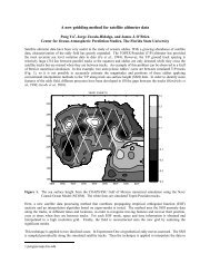
2.1 The <strong>Florida</strong> Big Bend Region doma<strong>in</strong>. Grey contours denote <strong>the</strong> isobaths<br />
from <strong>the</strong> high-resolution ocean model configured for <strong>the</strong> doma<strong>in</strong>. Triangles<br />
depict observational towers, open circles represent NDBC buoys, closed circles<br />
represent coastal sea level stations, dots depict Lagrangian particle seed<strong>in</strong>g<br />
locations, <strong>and</strong> <strong>the</strong> star denotes <strong>the</strong> location of <strong>the</strong> current profiler at site S. . 4<br />
3.1 Synoptic b<strong>and</strong> of <strong>the</strong> alongshore w<strong>in</strong>d stress power spectra dur<strong>in</strong>g <strong>the</strong> spr<strong>in</strong>g<br />
months, calculated us<strong>in</strong>g <strong>the</strong> maximum entropy method. . . . . . . . . . . . 19<br />
3.2 a)W<strong>in</strong>d stress rose for 7 years of spr<strong>in</strong>gtime w<strong>in</strong>d stresses taken from <strong>the</strong> ocean<br />
model simulation forced with CFSR, <strong>and</strong> b) box <strong>and</strong> whisker plots demonstrat<strong>in</strong>g<br />
<strong>the</strong> distribution of spr<strong>in</strong>gtime w<strong>in</strong>d stress orig<strong>in</strong>at<strong>in</strong>g from each direction.<br />
Vertical box edges <strong>in</strong>dicate <strong>the</strong> upper <strong>and</strong> lower quantiles, <strong>and</strong> hash marks<br />
designate 1.5 times <strong>the</strong> <strong>in</strong>terquartile range (IQR). Red l<strong>in</strong>es <strong>in</strong>dicate <strong>the</strong> median<br />
value. Direction of boxes on <strong>the</strong> w<strong>in</strong>d rose <strong>in</strong>dicate <strong>the</strong> direction from<br />
which <strong>the</strong> w<strong>in</strong>d stress orig<strong>in</strong>ates. . . . . . . . . . . . . . . . . . . . . . . . . 20<br />
3.3 Correlations, R, of modeled sea level to observed sea level at Cedar Key,<br />
Apalachicola, <strong>and</strong> Panama City dur<strong>in</strong>g each quarter (Jan-Mar; Apr-Jun; Jul-<br />
Sep; Oct-Dec). Red, green, blue, <strong>and</strong> black dots depict <strong>the</strong> correlation dur<strong>in</strong>g<br />
each quarter for BBROMS models forced by CFSR, COAMPS, NARR, <strong>and</strong><br />
NOGAPS, respectively. The colored numbers represent <strong>the</strong> maximum lagged<br />
correlations calculated for <strong>the</strong> entire 7-year time series, where numbers <strong>in</strong><br />
paren<strong>the</strong>ses show <strong>the</strong> number of hours lag at which <strong>the</strong> highest correlation is<br />
found. . . . . . . . . . . . . . . . . . . . . . . . . . . . . . . . . . . . . . . . 23<br />
3.4 Comparison of modeled <strong>and</strong> observed spr<strong>in</strong>gtime sub-<strong>in</strong>ertial sea level near<br />
Panama City, FL. Observations are shown <strong>in</strong> p<strong>in</strong>k, <strong>and</strong> red, green, blue, <strong>and</strong><br />
black l<strong>in</strong>es show modeled sea level from BBROMS simulations forced by CFSR,<br />
COAMPS, NARR, <strong>and</strong> NOGAPS, respectively. . . . . . . . . . . . . . . . . 25<br />
3.5 Same as figure 3.4, except for Apalachicola. . . . . . . . . . . . . . . . . . . 26<br />
3.6 Same as figure 3.4, except for Cedar Key. . . . . . . . . . . . . . . . . . . . . 27<br />
3.7 Annual mean sea surface temperatures ( o C) averaged across <strong>the</strong> BBROMS<br />
doma<strong>in</strong>. . . . . . . . . . . . . . . . . . . . . . . . . . . . . . . . . . . . . . . 28<br />
vi
3.8 Comparison of observed <strong>and</strong> modeled depth-averaged sub-<strong>in</strong>ertial spr<strong>in</strong>gtime<br />
alongshore currents at site N7. Values <strong>in</strong> <strong>the</strong> triplet <strong>in</strong>dicate <strong>the</strong> correlation R,<br />
<strong>the</strong> regression slope, <strong>and</strong> <strong>the</strong> difference between modeled mean <strong>and</strong> observed<br />
mean currents. Observations are shown <strong>in</strong> p<strong>in</strong>k, <strong>and</strong> red, green, blue, <strong>and</strong><br />
black l<strong>in</strong>es show modeled sea level from BBROMS simulations forced by CFSR,<br />
COAMPS, NARR, <strong>and</strong> NOGAPS, respectively. . . . . . . . . . . . . . . . . 32<br />
3.9 Same as figure 3.8, except for depth-averaged spr<strong>in</strong>gtime cross-shore currents. 33<br />
3.10 Comparison of mean observed <strong>and</strong> modeled spr<strong>in</strong>gtime currents at site N7.<br />
Observations are shown <strong>in</strong> p<strong>in</strong>k, <strong>and</strong> red, green, blue, <strong>and</strong> black l<strong>in</strong>es show<br />
modeled sea level from BBROMS simulations forced by CFSR, COAMPS,<br />
NARR, <strong>and</strong> NOGAPS, respectively. The 20th <strong>and</strong> 80th percentiles of <strong>the</strong><br />
observed flow are shown by dashed p<strong>in</strong>k l<strong>in</strong>es for each depth. . . . . . . . . 34<br />
3.11 Comparison of observed <strong>and</strong> modeled depth-averaged spr<strong>in</strong>gtime alongshore<br />
currents at site S. Values <strong>in</strong> <strong>the</strong> triplet <strong>in</strong>dicate <strong>the</strong> same set of values as <strong>in</strong><br />
figure 3.8. . . . . . . . . . . . . . . . . . . . . . . . . . . . . . . . . . . . . . 35<br />
3.12 Seven-year mean vertically averaged spr<strong>in</strong>g velocities for each contemporaneous<br />
model run. Current speeds are <strong>in</strong> color, with velocity vectors plotted every<br />
10 model grid po<strong>in</strong>ts. . . . . . . . . . . . . . . . . . . . . . . . . . . . . . . . 37<br />
3.13 Same as figure 3.12, except for seven-year mean near-surface velocities. . . . 38<br />
3.14 Same as figure 3.12, except for seven-year mean near-bottom velocities. . . . 39<br />
3.15 Yearly mean spr<strong>in</strong>gtime depth-averaged velocities for <strong>the</strong> CFSR-forced BBROMS<br />
simulation. Colors represent <strong>the</strong> current speed, <strong>and</strong> arrows depict <strong>the</strong> mean<br />
depth-averaged velocities, plotted every 10 model grid po<strong>in</strong>ts. . . . . . . . . . 43<br />
3.16 Conditionally-averaged flow fields for flow dur<strong>in</strong>g each w<strong>in</strong>d regime. Averages<br />
are calculated over all times dur<strong>in</strong>g Feb-May (for all 7 years) when <strong>the</strong> w<strong>in</strong>d<br />
orig<strong>in</strong>ated from each quadrant respective quadrant. Averages are <strong>the</strong>n scaled<br />
by <strong>the</strong> percentage of time that <strong>the</strong> w<strong>in</strong>ds orig<strong>in</strong>ated from that quadrant over<br />
<strong>the</strong> entire 7-year spr<strong>in</strong>g period. Scale arrows are not given as <strong>the</strong> scale value<br />
is arbitrary. . . . . . . . . . . . . . . . . . . . . . . . . . . . . . . . . . . . . 45<br />
3.17 Same as figure 3.12, except for flow only dur<strong>in</strong>g (top) upwell<strong>in</strong>g-favorable w<strong>in</strong>ds<br />
or (bottom) downwell<strong>in</strong>g-favorable w<strong>in</strong>ds. . . . . . . . . . . . . . . . . . . . 46<br />
3.18 Same as figure 3.12, except for flow only dur<strong>in</strong>g both upwell<strong>in</strong>g-favorable <strong>and</strong><br />
downwell<strong>in</strong>g-favorable w<strong>in</strong>ds. . . . . . . . . . . . . . . . . . . . . . . . . . . 47<br />
4.1 Color represents <strong>the</strong> Rossby number for flow dur<strong>in</strong>g northwesterly w<strong>in</strong>ds (leftt)<br />
<strong>and</strong> dur<strong>in</strong>g sou<strong>the</strong>asterly w<strong>in</strong>ds (right). Grey contours show <strong>the</strong> potential<br />
vorticity of <strong>the</strong> flow <strong>and</strong> black contours are f/h. . . . . . . . . . . . . . . . . 53<br />
vii
4.2 Colors denote mean values of ∆ζ/(ζ + f) <strong>and</strong> contours depict mean values<br />
of ∆h/h. Values are calculated based by averag<strong>in</strong>g values at each location<br />
follow<strong>in</strong>g all 1,467,648 particle trajectories. . . . . . . . . . . . . . . . . . . . 57<br />
4.3 Density of particles advected through each 1/10 o x 1/10 o box with <strong>the</strong> LTRANS<br />
simulation us<strong>in</strong>g ocean model fields from <strong>the</strong> CFSR-forced BBROMS. Colors<br />
denote <strong>the</strong> percentage of all particles over <strong>the</strong> 7-year period to ever go through<br />
each box at some po<strong>in</strong>t dur<strong>in</strong>g <strong>the</strong>ir advection. Areas without boxes conta<strong>in</strong><br />
less than 1% of <strong>the</strong> particles advected . . . . . . . . . . . . . . . . . . . . . . 58<br />
4.4 Same as figure 4.3, except separated for each year us<strong>in</strong>g <strong>the</strong> CFSR-forced<br />
BBROMS simulation <strong>and</strong> LTRANS. . . . . . . . . . . . . . . . . . . . . . . . 60<br />
4.5 Same as figure 4.3, except only for particles who successfully reach <strong>the</strong> 10m<br />
isobath dur<strong>in</strong>g <strong>the</strong>ir advection. . . . . . . . . . . . . . . . . . . . . . . . . . 61<br />
4.6 Dots denote <strong>the</strong> particle seed<strong>in</strong>g locations, <strong>and</strong> are colored based on <strong>the</strong> percentage<br />
of all particles released from each location that successfully reach <strong>the</strong><br />
10m isobath at some po<strong>in</strong>t dur<strong>in</strong>g <strong>the</strong>ir advection period. The total number<br />
of particles orig<strong>in</strong>at<strong>in</strong>g from each seed<strong>in</strong>g location is 9,408. . . . . . . . . . . 63<br />
viii
LIST OF ABBREVIATIONS<br />
ADCP Acoustic Doppler current profiler<br />
AWAC Acoustic wave <strong>and</strong> current<br />
BBR Big Bend region<br />
BBROMS Big Bend regional ocean model<strong>in</strong>g system<br />
CFSR Climate System Forecast Reanalysis<br />
COAMPS Coupled Ocean / Atmosphere Mesoscale Prediction System<br />
CSB Cape San Blas<br />
CSG Cape St. George<br />
DEM Digital Elevation Model<br />
ENSO El Niño / Sou<strong>the</strong>rn Oscillation<br />
FPS <strong>Florida</strong> Panh<strong>and</strong>le Shelf<br />
GODAE Global Ocean Data Assimilation Experiment<br />
GOM Gulf of Mexico<br />
HYCOM Hybrid Coord<strong>in</strong>ate Ocean Model<br />
IQR Interquartile range<br />
LC Loop Current<br />
LTRANS Larval <strong>transport</strong> Lagrangian model<br />
MISST Multi-sensor improved sea surface temperature<br />
MPDATA Multidimensional positive def<strong>in</strong>ite advection <strong>transport</strong> algorithm<br />
MSMR Madison Swanson Mar<strong>in</strong>e Reserve<br />
NARR North American Regional Reanalysis<br />
NCEP National Center for Environmental Prediction<br />
NCODA Navy Coupled Ocean Data Assimilation<br />
NDBC National Data Buoy Center<br />
NEGOM Nor<strong>the</strong>astern Gulf of Mexico<br />
NGDC National Geophysical Data Center<br />
NOAA National Oceanic <strong>and</strong> Atmospheric Adm<strong>in</strong>istration<br />
NOGAPS Navy Operational Global Atmospheric Prediction System<br />
NRL Naval Research Laboratory<br />
PLD Pelagic <strong>larval</strong> duration<br />
PV Potential vorticity<br />
ROMS Regional ocean model<strong>in</strong>g system<br />
rmse Root mean squared error<br />
SST Sea surface temperature<br />
WFS West <strong>Florida</strong> shelf<br />
ix
ABSTRACT<br />
The goal of this study is to quantify <strong>the</strong> <strong>transport</strong> <strong>mechanisms</strong> <strong>in</strong> <strong>the</strong> <strong>Florida</strong> Big Bend Re-<br />
gion that contribute to reef fish productivity as a function of <strong>the</strong> regional physical oceanog-<br />
raphy. The primary focus of <strong>the</strong> research is to identify pathways responsible for <strong>transport</strong><strong>in</strong>g<br />
gag grouper larvae from <strong>the</strong>ir offshore spawn<strong>in</strong>g grounds to <strong>in</strong>shore seagrass nurseries. More<br />
specifically, <strong>the</strong> role of variable w<strong>in</strong>d stress <strong>and</strong> <strong>the</strong> conservation of potential vorticity are<br />
<strong>in</strong>vestigated for <strong>the</strong>ir role <strong>in</strong> sett<strong>in</strong>g <strong>the</strong> net across-shelf <strong>transport</strong>. The primary tool used<br />
to address <strong>the</strong>se goals is a very high horizontal resolution (800-900m) numerical ocean<br />
model configured for <strong>the</strong> region <strong>and</strong> nested with<strong>in</strong> <strong>the</strong> data-assimilative Gulf of Mexico Hy-<br />
brid Coord<strong>in</strong>ate Ocean Model. Four contemporaneous simulations us<strong>in</strong>g this ocean model<br />
are forced with different atmospheric products of vary<strong>in</strong>g spatial <strong>and</strong> temporal resolution.<br />
Significant cross-shelf flow is generated dur<strong>in</strong>g upwell<strong>in</strong>g-favorable w<strong>in</strong>d events, <strong>and</strong> <strong>the</strong><br />
mean spr<strong>in</strong>gtime shelf circulation is set by <strong>the</strong> rectification of flow dur<strong>in</strong>g northwesterly<br />
or sou<strong>the</strong>asterly-directed w<strong>in</strong>d stress. A Lagrangian particle advection model is used as<br />
a proxy for <strong>the</strong> <strong>larval</strong> migration, <strong>in</strong> order to determ<strong>in</strong>e <strong>the</strong> physical pathways for onshore<br />
<strong>transport</strong>. Particle advection experiments <strong>in</strong>dicate that <strong>the</strong> flow is mostly barotropic <strong>and</strong><br />
conserves potential vorticity, lead<strong>in</strong>g to cross-isobath movement dur<strong>in</strong>g northwesterly w<strong>in</strong>ds.<br />
While <strong>the</strong>re is significant <strong>in</strong>terannual variability <strong>in</strong> <strong>the</strong> distribution of particles across <strong>the</strong><br />
shelf, <strong>the</strong> primary pathway by which particles are able to reach <strong>the</strong> nearshore environment<br />
is presented. The results also <strong>in</strong>dicate that <strong>the</strong> preferred release locations for particles that<br />
successfully arrive <strong>in</strong>shore co<strong>in</strong>cide with a known gag spawn<strong>in</strong>g aggregation site. The results<br />
presented <strong>in</strong> this dissertation provide, for <strong>the</strong> first time, a description of <strong>the</strong> <strong>mechanisms</strong> by<br />
which onshore <strong>transport</strong> is possible from gag spawn<strong>in</strong>g sites at <strong>the</strong> shelf break to seagrass<br />
nurseries at <strong>the</strong> coast.<br />
x
CHAPTER 1<br />
INTRODUCTION<br />
The Big Bend region (BBR) of <strong>Florida</strong> <strong>in</strong> <strong>the</strong> nor<strong>the</strong>astern Gulf of Mexico (NEGOM)<br />
exists at <strong>the</strong> juncture of <strong>the</strong> <strong>Florida</strong> Pen<strong>in</strong>sula <strong>and</strong> <strong>the</strong> <strong>Florida</strong> Panh<strong>and</strong>le, <strong>and</strong> where <strong>the</strong><br />
coastl<strong>in</strong>e orientation changes by roughly 90 o . The vast expanses of sea grass meadows along<br />
<strong>the</strong> coastl<strong>in</strong>e <strong>and</strong> <strong>the</strong> numerous reefs across <strong>the</strong> BBR provide both nursery habitats <strong>and</strong><br />
spawn<strong>in</strong>g sites for a plethora of mar<strong>in</strong>e species. These ecologically diverse <strong>and</strong> economically<br />
productive mar<strong>in</strong>e ecosystems of <strong>the</strong> BBR have been studied for fisheries production (e.g.<br />
Hood <strong>and</strong> Schlieder 1992; Koenig <strong>and</strong> Coleman 1998; Koenig et al. 2000; Gentner 2009).<br />
Commercial <strong>and</strong> recreational fish<strong>in</strong>g <strong>in</strong> <strong>the</strong> Gulf of Mexico (GOM henceforth, or sim-<br />
ply <strong>the</strong> Gulf) has raised considerable concern <strong>in</strong> response to reductions <strong>in</strong> both adult fish<br />
abundance <strong>and</strong> juvenile populations, where recreational fish<strong>in</strong>g accounts for over 60% of<br />
annual l<strong>and</strong><strong>in</strong>gs of certa<strong>in</strong> fish species (Coleman et al. 2004). While fish<strong>in</strong>g pressures affect<br />
<strong>the</strong> abundance of adult fish, <strong>the</strong> density-<strong>in</strong>dependent processes that occur dur<strong>in</strong>g <strong>the</strong>ir egg,<br />
<strong>larval</strong>, <strong>and</strong> early juvenile stages are significant <strong>in</strong> determ<strong>in</strong><strong>in</strong>g <strong>the</strong> <strong>in</strong>terannual variability<br />
<strong>in</strong> recruitment (Rothschild 1986; Chambers <strong>and</strong> Trippel 1997). Thus, underst<strong>and</strong><strong>in</strong>g re-<br />
cruitment processes of fish species is crucial for <strong>the</strong>ir effective management (Fitzhugh et al.<br />
2005).<br />
The physical oceanographic state can largely affect <strong>the</strong> egg <strong>and</strong> <strong>larval</strong> stages of reef fish<br />
development by sett<strong>in</strong>g <strong>the</strong>ir dispersion patterns as well as <strong>in</strong>fluenc<strong>in</strong>g locations conta<strong>in</strong><strong>in</strong>g<br />
available food (Rothschild <strong>and</strong> Osborn 1988; Werner et al. 1997). With motions of fertilized<br />
eggs <strong>and</strong> many early-stage larvae rema<strong>in</strong><strong>in</strong>g largely planktonic (Norcross <strong>and</strong> Shaw 1984),<br />
ocean currents may provide most of <strong>the</strong>ir horizontal dispersion. Fur<strong>the</strong>rmore, <strong>the</strong> circulation<br />
can set <strong>the</strong> distribution of food sources <strong>in</strong> <strong>the</strong> region, which mostly come from <strong>the</strong> nutrient-<br />
1
laden, high-chlorophyll coastal waters or via nutrient fluxes from <strong>the</strong> deep-ocean (He <strong>and</strong><br />
Weisberg 2003). By mov<strong>in</strong>g fish eggs <strong>and</strong> larvae to or from areas that are conducive for<br />
survival, <strong>the</strong> circulation can directly <strong>in</strong>fluence <strong>the</strong> recruitment <strong>and</strong> year-class strength of a<br />
given species (Norcross <strong>and</strong> Shaw 1984).<br />
One particular species <strong>in</strong> <strong>the</strong> BBR that relies on <strong>the</strong> circulation for <strong>the</strong> pelagic stage of<br />
its early life cycle is <strong>the</strong> gag grouper (Mycteroperca microlepis; Keener et al. 1988; Fitzhugh<br />
et al. 2005; Koenig <strong>and</strong> Coleman 1998). Indeed, gag is among <strong>the</strong> most valuable f<strong>in</strong>fish <strong>in</strong><br />
<strong>the</strong> region, as it provides over $100 million <strong>in</strong> value added <strong>and</strong> over $60 million <strong>in</strong> <strong>in</strong>come<br />
to <strong>the</strong> economy of <strong>the</strong> sou<strong>the</strong>astern United States from recreational fish<strong>in</strong>g alone (Gentner<br />
2009). Despite <strong>the</strong> economic importance of <strong>the</strong> gag fishery <strong>and</strong> <strong>the</strong> gag’s presence as a top-<br />
level predator, <strong>the</strong>re rema<strong>in</strong>s scarce knowledge about <strong>the</strong> early pre-settlement life stages<br />
of this particular fish. Adult gag spawn on offshore reefs along <strong>the</strong> cont<strong>in</strong>ental shelf break<br />
each spr<strong>in</strong>g (February-April; Hood <strong>and</strong> Schlieder 1992; Coleman et al. 1996), after which<br />
<strong>the</strong>ir larvae are <strong>transport</strong>ed across <strong>the</strong> shelf until eventually settl<strong>in</strong>g as juveniles <strong>in</strong> sea<br />
grass nursery habitats along <strong>the</strong> coast (Koenig <strong>and</strong> Coleman 1998). However, <strong>the</strong> physical<br />
<strong>mechanisms</strong> responsible for this onshore <strong>larval</strong> <strong>transport</strong> rema<strong>in</strong> unknown. This emphasizes<br />
that a 4-dimensional underst<strong>and</strong><strong>in</strong>g of <strong>the</strong> ocean circulation is needed <strong>in</strong> order to underst<strong>and</strong><br />
<strong>the</strong> processes affect<strong>in</strong>g <strong>larval</strong> dispersion <strong>in</strong> <strong>the</strong> BBR (Fitzhugh et al. 2005). Underst<strong>and</strong><strong>in</strong>g<br />
<strong>the</strong>se processes a priori can eventually aid <strong>the</strong> management of <strong>the</strong> gag fishery by improv<strong>in</strong>g<br />
predictions of <strong>the</strong> number of successful recruits from year to year.<br />
The material presented <strong>in</strong> this dissertation fills <strong>the</strong> need for a 4-dimensional underst<strong>and</strong>-<br />
<strong>in</strong>g of circulation features <strong>and</strong> <strong>transport</strong> <strong>mechanisms</strong> through <strong>the</strong> use of high-resolution<br />
ocean model<strong>in</strong>g experiments. The follow<strong>in</strong>g section provides a review of previous studies,<br />
a statement of <strong>the</strong> rema<strong>in</strong><strong>in</strong>g open questions, <strong>and</strong> <strong>the</strong> specific objectives addressed <strong>in</strong> this<br />
dissertation.<br />
2
CHAPTER 2<br />
BACKGROUND<br />
The Gulf of Mexico is a semi-enclosed bas<strong>in</strong> connected to <strong>the</strong> Atlantic Ocean by <strong>the</strong> Straits<br />
of <strong>Florida</strong> <strong>and</strong> to <strong>the</strong> Caribbean Sea via <strong>the</strong> Yucatan Channel (He <strong>and</strong> Weisberg 2002a).<br />
The GOM features a deep <strong>in</strong>terior (depths > 4km), <strong>and</strong> cont<strong>in</strong>ental shelves surround<strong>in</strong>g<br />
nearly <strong>the</strong> entire bas<strong>in</strong>. The shelves are of variable width <strong>and</strong> <strong>the</strong>ir bathymetries are of<br />
vary<strong>in</strong>g complexity. In <strong>the</strong> NEGOM, <strong>the</strong> cont<strong>in</strong>ental shelves are particularly noteworthy,<br />
where <strong>the</strong> West <strong>Florida</strong> shelf (WFS) has one of <strong>the</strong> widest shelves <strong>in</strong> <strong>the</strong> Gulf (150 - 200 km<br />
wide) adjacent to <strong>the</strong> relatively narrow (40km at its narrowest po<strong>in</strong>t) <strong>Florida</strong> Panh<strong>and</strong>le<br />
Shelf (FPS). The transition between <strong>the</strong>se two shelves occurs <strong>in</strong> <strong>the</strong> BBR offshore of Cape<br />
San Blas (CSB) <strong>and</strong> Cape St. George (CSG), where <strong>the</strong> isobaths converge <strong>and</strong> undergo<br />
tight curvature (figure 2.1).<br />
While <strong>the</strong> BBR has no official boundaries, it is characterized for this study by <strong>the</strong><br />
notable bend <strong>in</strong> <strong>the</strong> <strong>Florida</strong> coastl<strong>in</strong>e rang<strong>in</strong>g from St. Andrew’s Bay <strong>in</strong> <strong>the</strong> West along <strong>the</strong><br />
coast to roughly Chassahowitzka Bay <strong>in</strong> <strong>the</strong> South. The shelf break features numerous reefs<br />
<strong>and</strong> productive spawn<strong>in</strong>g grounds for many warm-temperate reef fish, <strong>in</strong>clud<strong>in</strong>g <strong>the</strong> gag<br />
grouper (Koenig <strong>and</strong> Coleman 1998), <strong>and</strong> <strong>the</strong> extensive seagrass beds near <strong>the</strong> coastl<strong>in</strong>e<br />
provide habitats for many f<strong>in</strong>fish <strong>and</strong> shellfish populations of significant economic value<br />
(Morey et al. 2009). There are several major rivers that dra<strong>in</strong> <strong>in</strong>to <strong>the</strong> region, namely <strong>the</strong><br />
Apalachicola, Choctawhatchee, <strong>and</strong> Suwannee Rivers. The Apalachicola River is by far<br />
<strong>the</strong> largest (annual mean discharge 736 m 3 /s; Morey et al. 2009), <strong>and</strong> perhaps <strong>the</strong> most<br />
<strong>in</strong>fluential river <strong>in</strong> <strong>the</strong> region, because it is considered to be a key source for <strong>the</strong> nutrient<br />
distribution across <strong>the</strong> WFS dur<strong>in</strong>g <strong>the</strong> late w<strong>in</strong>ter <strong>and</strong> early spr<strong>in</strong>g (Gilbes et al. 1996;<br />
Morey et al. 2009).<br />
3
Figure 2.1: The <strong>Florida</strong> Big Bend Region doma<strong>in</strong>. Grey contours denote <strong>the</strong> isobaths<br />
from <strong>the</strong> high-resolution ocean model configured for <strong>the</strong> doma<strong>in</strong>. Triangles<br />
depict observational towers, open circles represent NDBC buoys, closed circles represent<br />
coastal sea level stations, dots depict Lagrangian particle seed<strong>in</strong>g locations,<br />
<strong>and</strong> <strong>the</strong> star denotes <strong>the</strong> location of <strong>the</strong> current profiler at site S.<br />
While Morey et al. (2009) note that <strong>the</strong> impacts of <strong>the</strong> nutrient <strong>and</strong> freshwater <strong>in</strong>puts<br />
from <strong>the</strong> Apalachicola River on <strong>the</strong> mar<strong>in</strong>e ecosystems rema<strong>in</strong> unclear, <strong>the</strong> implications of<br />
<strong>the</strong>ir study suggest that such high nutrient concentrations (allow<strong>in</strong>g for <strong>in</strong>creased primary<br />
production), contribute to <strong>in</strong>creased food availability for ichthyoplankton across <strong>the</strong> NE-<br />
GOM shelf. Due to <strong>the</strong> direct relationship between food availability <strong>and</strong> recruitment class<br />
size (Cush<strong>in</strong>g 1975, 1990), <strong>the</strong> nutrient-laden waters of <strong>the</strong> Apalachicola River are consid-<br />
ered to be a large contributor to <strong>the</strong> regional fishery. Fur<strong>the</strong>rmore, s<strong>in</strong>ce <strong>the</strong> BBR is one of<br />
few regions on <strong>the</strong> WFS where upwelled deep water <strong>in</strong>teracts with coastal waters, <strong>the</strong>se two<br />
sources of high-nutrient waters could enable <strong>the</strong> <strong>Florida</strong> Middle Grounds fishery to rema<strong>in</strong><br />
so productive (He <strong>and</strong> Weisberg 2002b).<br />
The extensive seagrass beds of <strong>the</strong> BBR can exist <strong>in</strong> depths up to 20m, <strong>and</strong> to distances<br />
4
of up to 50 km offshore (Iverson <strong>and</strong> Bittaker 1986; Cont<strong>in</strong>ental Shelf Associates 1997).<br />
However, <strong>the</strong>ir coverage is not always cont<strong>in</strong>uous to those depths <strong>and</strong> distances offshore, <strong>and</strong><br />
<strong>the</strong>y can be significantly affected by flood-stage river outflow <strong>and</strong> tropical storms (Carlson<br />
et al. 2010).<br />
2.1 Gag Grouper<br />
The gag grouper (Family Serrendane, subfamily Ep<strong>in</strong>ephel<strong>in</strong>ae) is a common protogy-<br />
nous hermaphrodite. Adult gag spawn as early as January <strong>and</strong> <strong>in</strong>to April on hard relief<br />
bottom or reefs along <strong>the</strong> shelf break (50-90 m depth; Coleman et al. 1996; Koenig et al.<br />
2000; Fitzhugh et al. 2005), with peak spawn<strong>in</strong>g occurr<strong>in</strong>g <strong>in</strong> February <strong>and</strong> March (Hood<br />
<strong>and</strong> Schlieder 1992). Their larvae spend anywhere from 30-60 days (mean ∼ 43 days) <strong>in</strong> <strong>the</strong><br />
water column before settlement (a period known as <strong>the</strong>ir pelagic <strong>larval</strong> duration or PLD)<br />
<strong>in</strong> seagrass habitats along <strong>the</strong> <strong>Florida</strong> coast some 70-600 km away (Koenig <strong>and</strong> Coleman<br />
1998; Fitzhugh et al. 2005). At this stage, <strong>the</strong> gag metamorphose <strong>in</strong>to juveniles <strong>and</strong> take on<br />
a benthic existence (Mullaney <strong>and</strong> Gale 1996; Koenig <strong>and</strong> Coleman 1998). The year-class<br />
strength of <strong>the</strong> local fishery is strongly correlated with juvenile abundance <strong>in</strong> <strong>the</strong> seagrass<br />
habitats near <strong>the</strong> coast, which can vary 200 fold between high <strong>and</strong> low settlement years<br />
(Fitzhugh et al. 2005). However, while knowledge of spawn<strong>in</strong>g characteristics <strong>and</strong> settle-<br />
ment patterns have been documented <strong>in</strong> detail (Coleman et al. 1996; Koenig <strong>and</strong> Coleman<br />
1998; Koenig et al. 2000; Fitzhugh et al. 2005), <strong>the</strong>re rema<strong>in</strong>s a large gap <strong>in</strong> <strong>the</strong> scientific<br />
knowledge of gag larvae dur<strong>in</strong>g <strong>the</strong> time of <strong>the</strong>ir <strong>in</strong>gress.<br />
In an attempt to bridge this gap, sampl<strong>in</strong>g efforts have been aimed at observ<strong>in</strong>g var-<br />
ious ichthyoplankton across <strong>the</strong> NEGOM shelf <strong>and</strong> o<strong>the</strong>r areas where gag are known to<br />
spawn (SEAMAP, <strong>in</strong> coord<strong>in</strong>ation with <strong>the</strong> National Mar<strong>in</strong>e Fisheries Service). Although<br />
<strong>the</strong> Serranidae are found to be one of <strong>the</strong> more abundant families taken <strong>in</strong> collections of<br />
ichthyoplankton across <strong>the</strong> sou<strong>the</strong>astern coast of <strong>the</strong> US, <strong>the</strong> GOM, <strong>and</strong> <strong>the</strong> Caribbean, <strong>the</strong><br />
subfamily Ep<strong>in</strong>ephel<strong>in</strong>ae have not been found to be among those collected (Keener et al.<br />
1988). While gag are prevalent throughout <strong>the</strong> Gulf <strong>and</strong> off <strong>the</strong> Sou<strong>the</strong>astern coast of <strong>the</strong><br />
US, <strong>the</strong>ir spawn<strong>in</strong>g characteristics <strong>and</strong> <strong>larval</strong> behavioral patterns may vary by region. In<br />
fact, Fitzhugh et al. (2005) divided <strong>the</strong> eastern GOM <strong>in</strong>to three different regions based on<br />
5
gag spawn<strong>in</strong>g <strong>and</strong> settlement times. One <strong>the</strong>se regions designated by Fitzhugh et al. (2005)<br />
is <strong>the</strong> NEGOM, north of 28 o N <strong>and</strong> east of St. Andrew’s Bay.<br />
Keener et al. (1988) assessed <strong>the</strong> <strong>in</strong>gress of post<strong>larval</strong> (pre-settlement, but without<br />
juvenile pigmentation) gag through a South Carol<strong>in</strong>a barrier isl<strong>and</strong> <strong>in</strong>let, discover<strong>in</strong>g a<br />
relationship between lunar cycle, local tides, <strong>and</strong> <strong>in</strong>gress of gag. They f<strong>in</strong>d that <strong>the</strong> majority<br />
of postlarvae arrived <strong>in</strong>shore <strong>in</strong> <strong>the</strong> upper 3m of <strong>the</strong> water column at night, particularly <strong>in</strong><br />
association with <strong>the</strong> flood tide. The work by Keener et al. (1988) suggests that gag ei<strong>the</strong>r<br />
exhibit a diel vertical migration <strong>in</strong> order to rema<strong>in</strong> <strong>in</strong> preferred estuar<strong>in</strong>e locations, or simply<br />
settle immediately along <strong>the</strong> bottom <strong>in</strong> order to prevent seaward <strong>transport</strong> dur<strong>in</strong>g <strong>the</strong> ebb<br />
tide. That be<strong>in</strong>g said, Keener et al. (1988) do not assess those factors which <strong>transport</strong><br />
larvae from <strong>the</strong> offshore spawn<strong>in</strong>g locations to <strong>the</strong> nearshore <strong>in</strong>lets where post<strong>larval</strong> gag<br />
were captured. These <strong>transport</strong> processes on <strong>the</strong> shelf could likely be very different from<br />
<strong>the</strong> nearshore environment. This is particularly true <strong>in</strong> <strong>the</strong> NEGOM, where residual tidal<br />
currents are much weaker than at <strong>the</strong> same latitude <strong>in</strong> <strong>the</strong> Atlantic (He <strong>and</strong> Weisberg 2002a;<br />
Zetler <strong>and</strong> Hansen 1971).<br />
One of <strong>the</strong> only works to estimate <strong>the</strong> <strong>transport</strong> <strong>mechanisms</strong> of post<strong>larval</strong> gag <strong>in</strong> <strong>the</strong><br />
NEGOM is that by Fitzhugh et al. (2005). Their study uses <strong>in</strong>formation from juveniles<br />
collected <strong>in</strong> trawls through seagrass beds of <strong>the</strong> BBR (<strong>and</strong> also for a region south of 28 o N)<br />
<strong>in</strong> order to calculate temporal variations of spawn<strong>in</strong>g, fertilization, settlement, <strong>and</strong> PLD.<br />
In addition, <strong>the</strong>y constructed an empirical model of near-surface ocean currents from buoy<br />
observations to estimate horizontal near-surface <strong>transport</strong>. However, s<strong>in</strong>ce <strong>the</strong>re is no known<br />
knowledge of <strong>the</strong> vertical migratory behavior of gag larvae, <strong>the</strong>y only assessed <strong>the</strong> <strong>transport</strong><br />
of larvae that would rema<strong>in</strong> at <strong>the</strong> surface. Their conclusions revealed that near-surface<br />
currents driven by w<strong>in</strong>d forc<strong>in</strong>g alone could not provide <strong>the</strong> necessary mechanism for onshore<br />
<strong>transport</strong> anywhere along <strong>the</strong> WFS. They recommend <strong>the</strong> use of a fully three-dimensional<br />
physical model to properly assess <strong>the</strong> role of currents <strong>in</strong> all directions <strong>and</strong> at all depths.<br />
2.2 <strong>Circulation</strong> <strong>in</strong> <strong>the</strong> NEGOM<br />
The general circulation <strong>in</strong> <strong>the</strong> <strong>in</strong>terior of <strong>the</strong> GOM is largely driven by <strong>the</strong> <strong>in</strong>trusion of<br />
<strong>the</strong> western boundary current that enters through <strong>the</strong> Yucatan Channel, form<strong>in</strong>g <strong>the</strong> famous<br />
6
Loop Current (LC; Morey et al. 2005). The LC is <strong>the</strong> dom<strong>in</strong>ant energetic current <strong>in</strong> <strong>the</strong><br />
<strong>in</strong>terior GOM, <strong>and</strong> its <strong>in</strong>fluence on <strong>the</strong> circulation near <strong>the</strong> shelf break has been clearly<br />
documented (Weisberg et al. 1996; Meyers et al. 2001; He <strong>and</strong> Weisberg 2003; Barth et al.<br />
2008). He <strong>and</strong> Weisberg (2003) illustrate, through observations <strong>and</strong> some idealized model<br />
experiments, that currents along <strong>the</strong> WFS break are dom<strong>in</strong>antly controlled by <strong>in</strong>trusions<br />
of <strong>the</strong> LC upon <strong>the</strong> WFS. They fur<strong>the</strong>r suggest that <strong>the</strong> <strong>in</strong>fluence of <strong>the</strong>se <strong>in</strong>trusions are<br />
generally constricted to with<strong>in</strong> one radius of deformation (Rd ∼ 35 km), nearly 4-5 times<br />
narrower than <strong>the</strong> width of <strong>the</strong> WFS.<br />
The ocean’s circulation on cont<strong>in</strong>ental shelves is driven by a comb<strong>in</strong>ation of local surface<br />
forc<strong>in</strong>g, rivers, tides, <strong>and</strong> deep-ocean fluxes near <strong>the</strong> shelf break (Morey et al. 2005; Weisberg<br />
et al. 2005). However, <strong>the</strong> most dom<strong>in</strong>ant forc<strong>in</strong>g mechanism on <strong>the</strong> WFS <strong>and</strong> FPS is<br />
<strong>the</strong> w<strong>in</strong>d-driven component of this forc<strong>in</strong>g, as <strong>the</strong> NEGOM shelf circulation has a strong<br />
relationship with <strong>the</strong> local w<strong>in</strong>d stress (Mitchum <strong>and</strong> Clarke 1986; Morey <strong>and</strong> O’Brien 2002;<br />
Morey et al. 2005; Weisberg et al. 2005).<br />
From late fall through most of <strong>the</strong> spr<strong>in</strong>g, <strong>the</strong> w<strong>in</strong>ds are dom<strong>in</strong>ated by synoptic-scale<br />
wea<strong>the</strong>r systems (cold fronts; Clarke <strong>and</strong> Br<strong>in</strong>k 1985). Pre-frontal w<strong>in</strong>ds typically range<br />
from <strong>the</strong> south to <strong>the</strong> east, <strong>and</strong> upon <strong>the</strong> passage of cold fronts, <strong>the</strong>se w<strong>in</strong>ds will rotate<br />
relatively quickly (on <strong>the</strong> order of 10 m<strong>in</strong>utes to hours) to a westerly to nor<strong>the</strong>rly orig<strong>in</strong>. For<br />
<strong>the</strong> BBR, w<strong>in</strong>ds with a sou<strong>the</strong>asterly component are downwell<strong>in</strong>g-favorable, whereas w<strong>in</strong>ds<br />
with a northwesterly component are upwell<strong>in</strong>g-favorable, via <strong>the</strong> surface Ekman <strong>transport</strong>.<br />
Dur<strong>in</strong>g <strong>the</strong> summer months, <strong>the</strong> development of sea-breeze system provides <strong>the</strong> dom<strong>in</strong>ant<br />
variability of w<strong>in</strong>ds near <strong>the</strong> coast. However, as <strong>the</strong> sea-breeze system typically does not fully<br />
develop until <strong>the</strong> summer, it’s contribution to cross-shelf <strong>transport</strong> dur<strong>in</strong>g <strong>the</strong> spr<strong>in</strong>gtime<br />
is not discussed here. The strength, duration, <strong>and</strong> frequency of upwell<strong>in</strong>g-favorable w<strong>in</strong>ds<br />
varies highly on <strong>in</strong>terannual timescales. Weisberg <strong>and</strong> He (2003) illustrated that vary<strong>in</strong>g<br />
only <strong>the</strong> local mean monthly w<strong>in</strong>d stress <strong>in</strong> a model of <strong>the</strong> NEGOM for two separate years<br />
varied <strong>the</strong> shelf circulation patterns <strong>and</strong> <strong>the</strong> amount of upwell<strong>in</strong>g considerably. In fact, <strong>the</strong>y<br />
attributed most differences <strong>in</strong> circulation patterns <strong>and</strong> upwelled water properties on <strong>the</strong> shelf<br />
between <strong>the</strong> two years to <strong>the</strong> difference <strong>in</strong> <strong>the</strong> strength <strong>and</strong> duration of upwell<strong>in</strong>g-favorable<br />
w<strong>in</strong>d events.<br />
7
The transition from w<strong>in</strong>tertime synoptic-scale dom<strong>in</strong>ance to <strong>the</strong> more quiescent sum-<br />
mertime w<strong>in</strong>d patterns, along with a chang<strong>in</strong>g surface heat flux from net cool<strong>in</strong>g to net<br />
warm<strong>in</strong>g, manifests itself through changes <strong>in</strong> <strong>the</strong> ocean circulation. Indeed, <strong>the</strong> spr<strong>in</strong>g is<br />
a period when typical w<strong>in</strong>tertime horizontal stratification on <strong>the</strong> shelf gives way to verti-<br />
cal stratification, as surface heat<strong>in</strong>g <strong>in</strong>duces <strong>the</strong>rmocl<strong>in</strong>e development (Morey <strong>and</strong> O’Brien<br />
2002; He <strong>and</strong> Weisberg 2002b). Consequently, this spr<strong>in</strong>g transitionary period features a<br />
mid-shelf sou<strong>the</strong>astward current, cold <strong>and</strong> low sal<strong>in</strong>ity tongues, <strong>and</strong> a high chlorophyll plume<br />
(He <strong>and</strong> Weisberg 2002b). He <strong>and</strong> Weisberg (2002b) f<strong>in</strong>d that <strong>the</strong> w<strong>in</strong>d stress drives a circu-<br />
lation that is strongest near-shore <strong>in</strong> <strong>the</strong> BBR, while a cyclonic heat flux-<strong>in</strong>duced barocl<strong>in</strong>ic<br />
circulation adds constructively (destructively) to <strong>the</strong> mid-shelf (near-shore) w<strong>in</strong>d-driven<br />
circulation. They suggest that <strong>the</strong> <strong>in</strong>terplay between <strong>the</strong> local momentum <strong>and</strong> buoyancy<br />
forc<strong>in</strong>g creates a mid-shelf jet that flows sou<strong>the</strong>astward along <strong>the</strong> WFS (He <strong>and</strong> Weisberg<br />
2002b). As surface heat<strong>in</strong>g persists throughout <strong>the</strong> spr<strong>in</strong>g, <strong>the</strong> barocl<strong>in</strong>ic circulation recedes,<br />
a bifurcation of <strong>the</strong> coastal current near Cape San Blas disappears, <strong>and</strong> <strong>the</strong> jet streng<strong>the</strong>ns<br />
<strong>and</strong> moves slightly offshore (He <strong>and</strong> Weisberg 2002b).<br />
The barocl<strong>in</strong>ic circulation <strong>in</strong> <strong>the</strong> BBR has impacts beyond streng<strong>the</strong>n<strong>in</strong>g or relax<strong>in</strong>g<br />
<strong>the</strong> Big Bend Gyre. With <strong>the</strong> existence of upwell<strong>in</strong>g <strong>and</strong> net surface cool<strong>in</strong>g of coastal<br />
water dur<strong>in</strong>g <strong>the</strong> w<strong>in</strong>ter months, <strong>the</strong> comb<strong>in</strong>ed spr<strong>in</strong>gtime relaxation of negative surface<br />
heat flux <strong>and</strong> <strong>in</strong>creased river streamflow add to create a cold tongue that extends south<br />
along <strong>the</strong> mid-shelf (He <strong>and</strong> Weisberg 2002b). This cold tongue is a major contributor to<br />
<strong>the</strong> cyclonic circulation <strong>in</strong> <strong>the</strong> BBR. In fact, us<strong>in</strong>g modeled Lagrangian drifters, He <strong>and</strong><br />
Weisberg (2002b) f<strong>in</strong>d that <strong>the</strong> changes <strong>in</strong> hydrography dur<strong>in</strong>g <strong>the</strong> spr<strong>in</strong>g transition help<br />
promote onshore <strong>transport</strong> near <strong>the</strong> bottom from <strong>the</strong> shelf break to mid-shelf <strong>in</strong> <strong>the</strong> BBR.<br />
The presence of a river<strong>in</strong>e-<strong>in</strong>duced sal<strong>in</strong>ity front near <strong>the</strong> coast can allow shoreward<br />
flows to develop <strong>in</strong> <strong>the</strong> bottom layer <strong>and</strong> more complex flows near <strong>the</strong> <strong>in</strong>terface of <strong>the</strong><br />
front (Wea<strong>the</strong>rly <strong>and</strong> Thistle 1997; Lentz 2012). Under light w<strong>in</strong>ds, <strong>the</strong> buoyant current<br />
formed by <strong>the</strong> Apalachicola River will tend to <strong>the</strong> right, flow<strong>in</strong>g westward around <strong>the</strong> horn<br />
of CSB (Morey et al. 2009). However, as Morey et al. (2009) note, strong w<strong>in</strong>ds associated<br />
with <strong>the</strong> passage of atmospheric cold fronts force this low-sal<strong>in</strong>ity (<strong>and</strong> high chlorophyll)<br />
water offshore. This phenomenon, described as <strong>the</strong> ’Green River,’ only occurs after strong<br />
8
forc<strong>in</strong>g <strong>in</strong> conjunction with <strong>the</strong>se frontal passages (Gilbes et al. 1996; He <strong>and</strong> Weisberg<br />
2002b; Morey et al. 2009). The coastal waters, <strong>in</strong> conjunction with local surface cool<strong>in</strong>g,<br />
can produce areas of low temperature <strong>and</strong> sal<strong>in</strong>ity <strong>and</strong> high nutrient content on <strong>the</strong> <strong>in</strong>ner<br />
shelf. Then, mix<strong>in</strong>g with upwelled deep ocean water on <strong>the</strong> shelf produces <strong>the</strong> cool <strong>and</strong> low<br />
sal<strong>in</strong>ity tongues that can persist over <strong>the</strong> mid-shelf well <strong>in</strong>to <strong>the</strong> summer months (He <strong>and</strong><br />
Weisberg 2002b; Weisberg <strong>and</strong> He 2003).<br />
Tides <strong>in</strong> <strong>the</strong> Gulf of Mexico are relatively small <strong>in</strong> comparison with tidal amplitudes<br />
from o<strong>the</strong>r locations around <strong>the</strong> world at similar latitudes. The largest tidal constituents<br />
<strong>in</strong> <strong>the</strong> GOM are <strong>the</strong> diurnal tidal constituents (K1 <strong>and</strong> O1; He <strong>and</strong> Weisberg 2002a). This<br />
is <strong>in</strong> stark contrast to <strong>the</strong> Atlantic Coast at <strong>the</strong> same latitude, where <strong>the</strong> semidiurnal tide<br />
dom<strong>in</strong>ates (He <strong>and</strong> Weisberg 2002a; Zetler <strong>and</strong> Hansen 1971). The largest tides occur along<br />
<strong>the</strong> WFS <strong>and</strong> <strong>in</strong> <strong>the</strong> BBR, with <strong>the</strong> barotropic component rema<strong>in</strong><strong>in</strong>g relatively small (He<br />
<strong>and</strong> Weisberg 2002a; Gouillon et al. 2010). Tidal velocities rarely exceed a few cm/s, <strong>and</strong><br />
particle displacements from <strong>the</strong> barotropic tidal current rema<strong>in</strong> on <strong>the</strong> order of 10 km per<br />
month (He <strong>and</strong> Weisberg 2002a). Thus, while Keener et al. (1988) showed a relationship<br />
between tides <strong>and</strong> gag <strong>larval</strong> <strong>transport</strong> <strong>in</strong> South Carol<strong>in</strong>a, <strong>the</strong>ir relatively small impact on<br />
<strong>the</strong> overall <strong>transport</strong> of materials on <strong>the</strong> NEGOM shelf excludes tides from be<strong>in</strong>g of primary<br />
<strong>in</strong>terest for this study.<br />
The observational record <strong>in</strong> <strong>the</strong> BBR rema<strong>in</strong>s sparse, with most observational efforts<br />
focused offshore of Tampa Bay on <strong>the</strong> WFS, or to <strong>the</strong> west near Louisiana (e.g. Niiler 1976;<br />
Mitchum <strong>and</strong> Sturges 1982; Mitchum <strong>and</strong> Clarke 1986; Weisberg et al. 1996; Meyers et al.<br />
2001; He <strong>and</strong> Weisberg 2002b). The more permanent observational networks rema<strong>in</strong> to <strong>the</strong><br />
west of Tampa Bay, south of <strong>the</strong> region of immediate <strong>in</strong>terest for this dissertation. However,<br />
results from <strong>the</strong>se observational programs provide useful <strong>in</strong>sight <strong>in</strong>to <strong>dynamics</strong> affect<strong>in</strong>g <strong>the</strong><br />
WFS circulation. For example, <strong>the</strong> <strong>in</strong>fluence of <strong>the</strong> LC on shelf break currents, <strong>and</strong> <strong>the</strong><br />
<strong>in</strong>shore extent to which <strong>the</strong> LC exerts its <strong>in</strong>fluence have been described by several different<br />
works (Barth et al. 2008; Meyers et al. 2001; Weisberg et al. 1996). Also, much of <strong>the</strong><br />
observational work has provided evidence that <strong>the</strong> WFS circulation <strong>and</strong> sea level variations<br />
are highly correlated with variations <strong>in</strong> <strong>the</strong> synoptic scale w<strong>in</strong>d stress (Mitchum <strong>and</strong> Clarke<br />
1986; He <strong>and</strong> Weisberg 2002b; Maksimova 2012). These observations are generally limited<br />
9
to ADCP records, coastal tide gauge data, <strong>and</strong> a few transects across <strong>the</strong> WFS.<br />
Several surface drifter experiments have taken place <strong>in</strong> <strong>the</strong> NEGOM, from <strong>the</strong> drifter<br />
bottle experiments <strong>in</strong> <strong>the</strong> 1960s <strong>and</strong> 1970s (Tolbert <strong>and</strong> Salsman 1964; Gaul 1967; Williams<br />
et al. 1977), to <strong>the</strong> extensive SCULP project run by <strong>the</strong> M<strong>in</strong>eral Management Service (MMS;<br />
Yang et al. 1999; Sturges et al. 2001; Ohlmann <strong>and</strong> Niiler 2005). The major f<strong>in</strong>d<strong>in</strong>g of <strong>the</strong>se<br />
results, particularly those from <strong>the</strong> SCULP project, is that virtually no drifters have ever<br />
arrived <strong>in</strong>shore along <strong>Florida</strong>’s west coast, south of Apalachicola. This led for this region<br />
with no drifter tracks to be aptly named ”The Forbidden Zone” by Yang et al. (1999), <strong>and</strong><br />
suggests that onshore <strong>transport</strong> likely occurs <strong>in</strong> layers o<strong>the</strong>r than <strong>the</strong> surface. In fact, Yang<br />
et al. (1999) suggest that onshore <strong>transport</strong> <strong>in</strong> <strong>the</strong> sou<strong>the</strong>rn portion of <strong>the</strong> BBR occurs<br />
<strong>in</strong> <strong>the</strong> bottom layer, due to a slight convergence of isobaths <strong>in</strong> this region. While <strong>the</strong>se<br />
works provide useful analysis of observations along <strong>the</strong> NEGOM shelf, a large gap rema<strong>in</strong>s<br />
<strong>in</strong> observations across <strong>the</strong> BBR, <strong>and</strong> questions regard<strong>in</strong>g cross-shelf <strong>transport</strong> have yet to<br />
be fully addressed.<br />
The overall lack of observations <strong>in</strong> <strong>the</strong> BBR has been somewhat bridged by numerous<br />
model<strong>in</strong>g studies of <strong>the</strong> region (e.g. Weisberg et al. 2001; He <strong>and</strong> Weisberg 2002b, 2003;<br />
Morey et al. 2005, 2009; Barth et al. 2007, 2008). A series of studies (e.g. He <strong>and</strong><br />
Weisberg 2002a,b, 2003; Weisberg et al. 2001) used a model configured for <strong>the</strong> eastern<br />
GOM to <strong>in</strong>vestigate different process studies on <strong>the</strong> WFS. These studies ma<strong>in</strong>ly focused on<br />
<strong>the</strong> general circulation across <strong>the</strong> NEGOM shelf, from Mississippi to <strong>the</strong> <strong>Florida</strong> Keys. In<br />
particular, <strong>the</strong>y assessed <strong>the</strong> role of w<strong>in</strong>d forc<strong>in</strong>g, surface heat fluxes, <strong>and</strong> tides on <strong>the</strong> general<br />
circulation of <strong>the</strong> NEGOM. In <strong>the</strong> process, He <strong>and</strong> Weisberg (2003, 2002b) also discussed<br />
<strong>the</strong> transitionary periods of Fall 1998 <strong>and</strong> Spr<strong>in</strong>g 1999, respectively. All of <strong>the</strong>se previous<br />
model<strong>in</strong>g studies provide a great foundation for <strong>the</strong> work to be presented <strong>in</strong> <strong>the</strong> follow<strong>in</strong>g<br />
sections, as <strong>the</strong>y describe many of <strong>the</strong> relevant circulation features <strong>and</strong> <strong>the</strong> contribution of<br />
vary<strong>in</strong>g forc<strong>in</strong>g <strong>mechanisms</strong> to <strong>the</strong> formation of those features.<br />
With <strong>the</strong> exception of <strong>the</strong> works by Morey et al. (2005, 2009), <strong>the</strong> only discussions of<br />
cross-shelf <strong>transport</strong> <strong>in</strong> <strong>the</strong> BBR from <strong>the</strong> aforementioned model<strong>in</strong>g studies rema<strong>in</strong> specu-<br />
lative. In fact, even Morey et al. (2009) were concerned only with <strong>the</strong> relationship between<br />
<strong>the</strong> cross-shelf <strong>transport</strong> of low-sal<strong>in</strong>ity waters <strong>and</strong> ocean color imagery <strong>in</strong> order to fur<strong>the</strong>r<br />
10
<strong>the</strong> underst<strong>and</strong><strong>in</strong>g of <strong>the</strong> ’Green River’ generation <strong>mechanisms</strong>. While <strong>the</strong>ir study implies<br />
several different consequences of this low-sal<strong>in</strong>ity / high chlorophyll content <strong>in</strong> regards to<br />
<strong>the</strong> regional fishery, <strong>the</strong> <strong>mechanisms</strong> for <strong>transport</strong> of materials from <strong>the</strong> shelf break to <strong>the</strong><br />
coast rema<strong>in</strong> largely undiscussed <strong>in</strong> previous works. One attempt to underst<strong>and</strong> <strong>the</strong> physi-<br />
cal <strong>transport</strong> <strong>mechanisms</strong> of gag larvae <strong>in</strong> <strong>the</strong> BBR is that by Fitzhugh et al. (2005). They<br />
f<strong>in</strong>d that, although surface <strong>transport</strong> is generally directed northward along <strong>the</strong> WFS, <strong>the</strong><br />
surface layer <strong>transport</strong> by w<strong>in</strong>d alone does not produce <strong>the</strong> necessary cross-shelf <strong>transport</strong><br />
for gag larvae, <strong>and</strong> concede that a fully three-dimensional approach at underst<strong>and</strong><strong>in</strong>g <strong>the</strong>se<br />
processes is needed.<br />
2.3 Research Overview<br />
This review of previous studies <strong>in</strong>dicates that a detailed knowledge of <strong>the</strong> physical trans-<br />
port processes <strong>in</strong> <strong>the</strong> BBR is needed <strong>in</strong> order to underst<strong>and</strong> <strong>the</strong> early stages of <strong>the</strong> gag<br />
grouper’s life cycle. While <strong>the</strong> tim<strong>in</strong>g <strong>and</strong> locations of gag spawn<strong>in</strong>g aggregations have<br />
been described (i.e. Coleman et al. 1996; Fitzhugh et al. 2005), <strong>the</strong>re rema<strong>in</strong>s a gap <strong>in</strong> <strong>the</strong><br />
previous studies about <strong>the</strong> processes affect<strong>in</strong>g gag grouper dur<strong>in</strong>g <strong>the</strong>ir time of <strong>in</strong>gress to<br />
<strong>the</strong> seagrass nurseries (Fitzhugh et al. 2005). It is understood that <strong>the</strong> shelf circulation<br />
dur<strong>in</strong>g <strong>the</strong> spr<strong>in</strong>g months is set largely by <strong>the</strong> local w<strong>in</strong>d stress, although it is unclear how<br />
<strong>the</strong> circulation <strong>in</strong> <strong>the</strong> BBR evolves <strong>in</strong> 3-dimensions <strong>and</strong> how it responds to higher frequency<br />
variations <strong>in</strong> <strong>the</strong> w<strong>in</strong>d stress. F<strong>in</strong>ally, it rema<strong>in</strong>s to be determ<strong>in</strong>ed how <strong>the</strong> circulation fea-<br />
tures <strong>in</strong> <strong>the</strong> region contribute to <strong>the</strong> onshore <strong>transport</strong> of gag larvae dur<strong>in</strong>g <strong>the</strong> spr<strong>in</strong>g. This<br />
dissertation aims to fill a portion of this gag <strong>in</strong> knowledge by assess<strong>in</strong>g <strong>the</strong> impact of <strong>the</strong><br />
physical <strong>transport</strong> on sett<strong>in</strong>g <strong>the</strong> distribution of materials across <strong>the</strong> shelf. In particular,<br />
this study focuses on three outst<strong>and</strong><strong>in</strong>g research questions:<br />
1. What is <strong>the</strong> <strong>in</strong>fluence of variable atmospheric w<strong>in</strong>d stress on <strong>the</strong> major circulation<br />
features of <strong>the</strong> <strong>Florida</strong> Big Bend shelf?<br />
2. What are <strong>the</strong> physical <strong>mechanisms</strong> by which cross-shelf <strong>transport</strong> is possible dur<strong>in</strong>g<br />
<strong>the</strong> spr<strong>in</strong>g months?<br />
3. Are <strong>the</strong> physical <strong>transport</strong> <strong>mechanisms</strong> <strong>in</strong> <strong>the</strong> BBR capable of provid<strong>in</strong>g <strong>the</strong> necessary<br />
<strong>transport</strong> for gag larvae from <strong>the</strong> shelf break to coastal seagrass nurseries?<br />
11
The results of this study are expected to provide a basic foundation for fisheries ecolo-<br />
gists to underst<strong>and</strong> <strong>the</strong> potential pathways by which gag larvae are able to arrive <strong>in</strong> <strong>the</strong>ir<br />
nursery habitats each spr<strong>in</strong>g. This will enable fur<strong>the</strong>r <strong>in</strong>terdiscipl<strong>in</strong>ary research <strong>in</strong>to <strong>the</strong><br />
physical characteristics <strong>and</strong> ecology of <strong>the</strong> region <strong>and</strong> will unlock a portion of <strong>the</strong> mystery<br />
that surrounds <strong>the</strong> early part of this particular reef fish’s life cycle. Also, s<strong>in</strong>ce this study<br />
focuses on <strong>the</strong> physical <strong>transport</strong> <strong>mechanisms</strong> <strong>in</strong> <strong>the</strong> region, <strong>the</strong> results are also expected<br />
to be applicable to <strong>the</strong> <strong>transport</strong> of a variety of environmentally-important materials (i.e.<br />
pollutants, oil spills, harmful algal blooms, etc.) <strong>in</strong>to <strong>the</strong> BBR. In chapter 3, <strong>the</strong> impact<br />
of w<strong>in</strong>d stress variability on <strong>the</strong> major shelf circulation features are discussed us<strong>in</strong>g four<br />
contemporaneous ocean model simulations. Then, <strong>in</strong> chapter 4, <strong>the</strong> <strong>mechanisms</strong> are deter-<br />
m<strong>in</strong>ed for which cross-shore <strong>transport</strong> is possible. The pathways by which <strong>the</strong>se <strong>mechanisms</strong><br />
allow for <strong>the</strong> necessary <strong>transport</strong> of gag larvae is also discussed. F<strong>in</strong>ally, conclusions <strong>and</strong><br />
<strong>the</strong> future of this work is discussed <strong>in</strong> chapter 5.<br />
12
CHAPTER 3<br />
THE IMPACT OF VARIABLE ATMOSPHERIC<br />
FORCING ON THE SPRINGTIME<br />
CIRCULATION IN THE BIG BEND REGION<br />
The BBR is a historically under-studied area of <strong>the</strong> world’s ocean, yet this region’s mar<strong>in</strong>e<br />
ecosystems rema<strong>in</strong> a viable economic source for <strong>the</strong> sou<strong>the</strong>astern United States. Valuable<br />
fish species <strong>in</strong> <strong>the</strong> region rely on <strong>the</strong> regional circulation for survival dur<strong>in</strong>g <strong>the</strong> early stages<br />
of <strong>the</strong>ir life cycle. The f<strong>in</strong>d<strong>in</strong>gs from previous studies <strong>in</strong> <strong>the</strong> region outl<strong>in</strong>ed <strong>in</strong> chapter 2<br />
<strong>in</strong>dicate that <strong>the</strong> primary driver of <strong>the</strong> shelf circulation on <strong>the</strong> WFS <strong>and</strong> BBR is <strong>the</strong> flux of<br />
momentum from <strong>the</strong> atmosphere. Thus, <strong>the</strong> aim of this chapter is to describe <strong>the</strong> variability<br />
of <strong>the</strong> w<strong>in</strong>d stress over <strong>the</strong> region, <strong>and</strong> to demonstrate how vary<strong>in</strong>g representations of <strong>the</strong><br />
atmospheric state affect <strong>the</strong> ocean circulation <strong>in</strong> <strong>the</strong> BBR. F<strong>in</strong>ally, this chapter describes <strong>the</strong><br />
dom<strong>in</strong>ant flow features dur<strong>in</strong>g <strong>the</strong> spr<strong>in</strong>gtime, <strong>and</strong> <strong>the</strong>ir variability on multiple scales. This<br />
is done by analyz<strong>in</strong>g various atmospheric products <strong>and</strong> through several contemporaneous<br />
ocean model simulations.<br />
3.1 Introduction<br />
The <strong>Florida</strong> BBR is an area that has lacked significant focus <strong>in</strong> previous studies of shelf<br />
circulation processes <strong>in</strong> <strong>the</strong> GOM. Section 2.2 <strong>in</strong>dicates that most studies have ei<strong>the</strong>r been<br />
relatively short-lived or have been concerned with flow features fur<strong>the</strong>r to <strong>the</strong> south or<br />
west, where major ports are located. However, <strong>the</strong> short-lived observational studies (e.g.<br />
Marmor<strong>in</strong>o 1983; Mitchum <strong>and</strong> Clarke 1986; Wea<strong>the</strong>rly <strong>and</strong> Thistle 1997) <strong>in</strong> <strong>the</strong> region<br />
have all <strong>in</strong>dicated that <strong>the</strong>re exists a strong relationship between <strong>the</strong> local w<strong>in</strong>d stress <strong>and</strong><br />
13
<strong>the</strong> shelf circulation, a f<strong>in</strong>d<strong>in</strong>g that is emphasized over broader spatial scales <strong>in</strong> several<br />
model<strong>in</strong>g studies whose doma<strong>in</strong>s <strong>in</strong>clude <strong>the</strong> BBR (e.g. Li <strong>and</strong> Weisberg 1999a,b; Morey<br />
et al. 2005; Weisberg et al. 2005). The observational studies mostly focus on <strong>the</strong> ocean’s<br />
response to large-scale, low frequency w<strong>in</strong>d forc<strong>in</strong>g, <strong>and</strong> not <strong>the</strong> response to w<strong>in</strong>ds that have<br />
higher spatial or temporal variability. This large-scale, low frequency variability dur<strong>in</strong>g <strong>the</strong><br />
spr<strong>in</strong>gtime is provided by <strong>the</strong> passage of cold fronts, which have phases of downwell<strong>in</strong>g (pre-<br />
fontal passage) <strong>and</strong> upwell<strong>in</strong>g (post-frontal passage) favorable w<strong>in</strong>d stress over <strong>the</strong> WFS <strong>and</strong><br />
BBR. The strength <strong>and</strong> frequency of upwell<strong>in</strong>g favorable events may vary on multiple time<br />
scales, <strong>and</strong> <strong>the</strong> response of <strong>the</strong> shelf circulation can be quite different based on <strong>the</strong> direction<br />
of <strong>the</strong> w<strong>in</strong>ds (Li <strong>and</strong> Weisberg 1999a,b).<br />
While <strong>the</strong> dom<strong>in</strong>ant variability <strong>in</strong> <strong>the</strong> spr<strong>in</strong>gtime occurs at synoptic scales, it is unclear<br />
from <strong>the</strong> previous literature what impact a higher degree of spatial <strong>and</strong> temporal variability<br />
<strong>in</strong> <strong>the</strong> w<strong>in</strong>ds may have on <strong>the</strong> shelf circulation. Weisberg et al. (2005) discuss <strong>the</strong> variability<br />
of <strong>the</strong> WFS circulation on multiple time scales (from synoptic scales to <strong>in</strong>terannual fluctu-<br />
ations). They f<strong>in</strong>d that <strong>the</strong> while <strong>the</strong> synoptic wea<strong>the</strong>r systems dom<strong>in</strong>ant <strong>the</strong> circulation<br />
features with<strong>in</strong> each season, <strong>the</strong>re are significant variations between seasons <strong>and</strong> between<br />
years. The <strong>in</strong>terannual fluctuations <strong>in</strong> <strong>the</strong> strength <strong>and</strong> frequency of frontal passages could<br />
be affected by large-scale changes <strong>in</strong> wea<strong>the</strong>r patterns, such as those associated with <strong>the</strong><br />
phase of el Niño / Sou<strong>the</strong>rn Oscillation (ENSO). The positive (negative) correlation be-<br />
tween ENSO phase <strong>and</strong> precipitation (500 hPa heights) over <strong>the</strong> sou<strong>the</strong>ast suggests that<br />
years with a positive ENSO phase (el Niño) years may expect stormier wea<strong>the</strong>r (i.e. more<br />
frontal passages; Hoerl<strong>in</strong>g <strong>and</strong> Kumar 2001; Ropelewski <strong>and</strong> Halpert 1986). Therefore, el<br />
Niño years may expect more frequent, <strong>and</strong> potentially stronger, frontal passages. For <strong>the</strong><br />
rema<strong>in</strong>der of this dissertation, <strong>the</strong> spr<strong>in</strong>g is def<strong>in</strong>ed as February through May, as this period<br />
of time covers most of <strong>the</strong> spawn<strong>in</strong>g <strong>and</strong> PLD for gag grouper <strong>in</strong> <strong>the</strong> BBR.<br />
It rema<strong>in</strong>s to be addressed how higher temporal or smaller spatial-scale variations <strong>in</strong> <strong>the</strong><br />
w<strong>in</strong>d stress affect <strong>the</strong> response of <strong>the</strong> coastal ocean circulation dur<strong>in</strong>g <strong>the</strong> spr<strong>in</strong>g months. In<br />
particular, <strong>the</strong> response of <strong>the</strong> shelf waters <strong>in</strong> <strong>the</strong> geometrically <strong>in</strong>trigu<strong>in</strong>g BBR rema<strong>in</strong> to<br />
be fully discussed from a fully 4-dimensional approach. Therefore, this chapter is focused on<br />
<strong>the</strong> impact of a vary<strong>in</strong>g atmospheric state on <strong>the</strong> major features of <strong>the</strong> spr<strong>in</strong>gtime BBR shelf<br />
14
circulation. In <strong>the</strong> follow<strong>in</strong>g sections, a description of <strong>the</strong> variability of spr<strong>in</strong>gtime w<strong>in</strong>ds<br />
over <strong>the</strong> BBR is given us<strong>in</strong>g various atmospheric products as vary<strong>in</strong>g atmospheric represen-<br />
tations. These products are used as surface forc<strong>in</strong>g for four contemporaneous ocean model<br />
simulations. Next, a comparison of model results to a variety of observational platforms <strong>in</strong><br />
<strong>the</strong> region is given. A description of <strong>the</strong> mean circulation features <strong>and</strong> <strong>the</strong> variability <strong>in</strong> <strong>the</strong><br />
flow on multiple time scales <strong>the</strong>n follows.<br />
3.2 W<strong>in</strong>d Variability<br />
One aim of this chapter is to underst<strong>and</strong> how variations <strong>in</strong> <strong>the</strong> dom<strong>in</strong>ant forc<strong>in</strong>g mech-<br />
anism over <strong>the</strong> BBR affect <strong>the</strong> major features of <strong>the</strong> shelf circulation. Therefore, vary<strong>in</strong>g<br />
manifestations of <strong>the</strong> atmospheric state are provided via output from four different atmo-<br />
spheric models of vary<strong>in</strong>g spatial <strong>and</strong> temporal resolution. Two of <strong>the</strong>se datasets are reanal-<br />
ysis products developed <strong>and</strong> operated by <strong>the</strong> National Center of Environmental Prediction’s<br />
(NCEP) Environmental Model<strong>in</strong>g Center, while <strong>the</strong> o<strong>the</strong>r two datasets are data-assimilative<br />
h<strong>in</strong>dcast / nowcast model runs developed <strong>and</strong> operated by <strong>the</strong> United States Naval Research<br />
Laboratory (NRL). Therefore, all four products are state-of-<strong>the</strong>-art prediction systems that<br />
are bound to observations through advanced assimilation schemes. In addition to vary<strong>in</strong>g<br />
model physics <strong>and</strong> assimilation methods, each product provides a different comb<strong>in</strong>ation of<br />
horizontal grid spac<strong>in</strong>g <strong>and</strong> temporal resolution (see table 3.1), allow<strong>in</strong>g <strong>the</strong> impact of vary-<br />
<strong>in</strong>g resolution on <strong>the</strong> result<strong>in</strong>g ocean circulation features to be assessed. The four different<br />
datasets will be discussed, along with <strong>the</strong> variability among <strong>and</strong> between <strong>the</strong>m. Compar-<br />
isons are made to regional meteorological observations from buoys to assess <strong>the</strong> accuracy<br />
of each product with respect to observations. The atmospheric datasets are <strong>the</strong>n used to<br />
force a regional ocean circulation model.<br />
3.2.1 Description of <strong>the</strong> datasets<br />
The two reanalysis products used <strong>in</strong> this study are <strong>the</strong> Climate Forecast System Re-<br />
analysis (CFSR) <strong>and</strong> <strong>the</strong> North American Regional Reanalysis (NARR). The CFSR is a<br />
global coupled ocean-atmosphere-l<strong>and</strong>-sea ice model<strong>in</strong>g system that uses <strong>the</strong> NCEP Global<br />
Data Assimilation System (GDAS), <strong>and</strong> is described <strong>in</strong> great detail <strong>in</strong> Saha <strong>and</strong> Coauthors<br />
15
(2006). It is <strong>the</strong> newest product of <strong>the</strong> four chosen models, which is notable <strong>in</strong> that it <strong>in</strong>-<br />
corporates more data <strong>in</strong>to its assimilation system (notably scatterometer w<strong>in</strong>ds <strong>and</strong> direct<br />
assimilation of satellite-derived radiances). This product also provides <strong>the</strong> highest temporal<br />
resolution (hourly) of <strong>the</strong> four atmospheric datasets. The hourly output fields are provided<br />
<strong>in</strong> <strong>the</strong> form of analysis fields every 6 hours, with hourly forecast fields for <strong>the</strong> <strong>in</strong>termediate<br />
time steps. The NARR is an atmosphere-l<strong>and</strong> hydrology coupled model, which is run for<br />
regional application to North America (for more details see Mes<strong>in</strong>ger <strong>and</strong> Coauthors 2006)<br />
at roughly 1/3 o horizontal grid spac<strong>in</strong>g <strong>and</strong> available at an output frequency of 3 hours.<br />
NARR is based on <strong>the</strong> NCEP Eta atmospheric model, <strong>and</strong> uses its associated 3D variational<br />
technique for assimilation of observations (Mes<strong>in</strong>ger <strong>and</strong> Coauthors 2006).<br />
The Navy Operational Global Atmospheric Prediction System (NOGAPS) <strong>and</strong> <strong>the</strong> Cou-<br />
pled Ocean/Atmosphere Mesoscale Prediction System (COAMPS) are operational, data-<br />
assimilative models available from <strong>the</strong> NRL (see Hogan <strong>and</strong> Rosmond 1991; Rosmond 1992;<br />
Hodur 1996). The NRL’s Central America COAMPS configuration is used <strong>in</strong> this study.<br />
It is run as an uncoupled atmospheric model us<strong>in</strong>g <strong>the</strong> Navy’s multivariate optimally <strong>in</strong>-<br />
terpolated (MVOI) data assimilation system (Goerss <strong>and</strong> Phoebus 1992; Barker 1992) <strong>and</strong><br />
provides <strong>the</strong> highest horizontal grid spac<strong>in</strong>g for this study, at 0.2 o . NOGAPS, which also<br />
uses <strong>the</strong> MVOI data assimilation system, has <strong>the</strong> coarsest grid spac<strong>in</strong>g for this study at 0.5 o ,<br />
with 3-hourly output. The NOGAPS is also used to force <strong>the</strong> 1/25 o GODAE Gulf of Mex-<br />
ico HYbrid Coord<strong>in</strong>ate Ocean Model (GOM HYCOM; Bleck 2002; Chassignet et al. 2007,<br />
2009; Chassignet 2011). As will be described <strong>in</strong> detail <strong>in</strong> section 3.3, <strong>the</strong> GOM HYCOM is<br />
used to set <strong>the</strong> open boundary conditions for an ocean model for <strong>the</strong> BBR. This makes <strong>the</strong><br />
<strong>in</strong>clusion of NOGAPS of <strong>in</strong>terest to this study <strong>in</strong> order use a consistent atmospheric forc<strong>in</strong>g<br />
across <strong>the</strong> model’s open boundaries.<br />
3.2.2 Discussion of <strong>the</strong> variability<br />
The w<strong>in</strong>ds from each atmospheric product are compared to observations from three<br />
mar<strong>in</strong>e observation platforms <strong>in</strong> <strong>the</strong> NEGOM (National Data Buoy Center [NDBC] buoys<br />
42036 <strong>and</strong> 42039, <strong>and</strong> SGOF1) over <strong>the</strong> period 2004-2010. W<strong>in</strong>ds are adjusted to a common<br />
10m above <strong>the</strong> surface us<strong>in</strong>g st<strong>and</strong>ard height adjustment procedures outl<strong>in</strong>ed by Liu <strong>and</strong><br />
16
Model Grid Temporal Range<br />
Spac<strong>in</strong>g Resolution<br />
CFSR T382 1 hour 1979-2009<br />
NARR ∼ 32.46 km 3 hour 1979 - Present<br />
NOGAPS 0.5 o x 0.5 o 3 hour 2003 - Present<br />
COAMPS 0.2 o x 0.2 o 3 hour 2003 - Present<br />
Table 3.1: Atmospheric model grid specifications.<br />
Tang (1996). Unless o<strong>the</strong>rwise mentioned, w<strong>in</strong>ds have been low-pass filtered us<strong>in</strong>g a cos<strong>in</strong>e-<br />
Lanczos filter (Emery <strong>and</strong> Thompson 2001) to remove variability at frequencies shorter than<br />
30 hours (result<strong>in</strong>g <strong>in</strong> sub-<strong>in</strong>ertial or low frequency variability; see Appendix B for more<br />
detail on <strong>the</strong> filter<strong>in</strong>g procedure).<br />
A list of <strong>the</strong> correlation coefficients <strong>and</strong> parameter estimates from a l<strong>in</strong>ear regression fit<br />
between modeled w<strong>in</strong>ds <strong>and</strong> observed w<strong>in</strong>ds over <strong>the</strong> entire 7-year period of 2004-2010 is<br />
given <strong>in</strong> table 3.2.2. Regression slopes that are close to unity <strong>in</strong>dicate that NOGAPS <strong>and</strong><br />
COAMPS estimate <strong>the</strong> strength of <strong>the</strong> observed w<strong>in</strong>ds well at sites 42039 <strong>and</strong> SGOF1, where<br />
<strong>the</strong> models only overestimate w<strong>in</strong>d speeds <strong>in</strong> <strong>the</strong> low-w<strong>in</strong>d environment by about 0.4-0.6<br />
ms −1 . NOGAPS <strong>and</strong> COAMPS under-estimate w<strong>in</strong>d speed <strong>in</strong> <strong>the</strong> high-w<strong>in</strong>d environment<br />
by up to 1 ms −1 at <strong>the</strong>se locations. NOGAPS does particularly poor among <strong>the</strong> products at<br />
captur<strong>in</strong>g <strong>the</strong> variability <strong>in</strong> w<strong>in</strong>d stress at 42036 (R 2 = 0.551), however <strong>in</strong>creased R 2 values<br />
at 42039 <strong>and</strong> SGOF1 <strong>in</strong>dicate that it captures <strong>the</strong> variability of observed w<strong>in</strong>ds much better<br />
at <strong>the</strong>se locations. COAMPS captures <strong>the</strong> variability at all observation locations well, with<br />
R 2 values above 0.82.<br />
CFSR estimates <strong>the</strong> strength of <strong>the</strong> w<strong>in</strong>ds well <strong>in</strong> <strong>the</strong> mid to high w<strong>in</strong>d strength environ-<br />
ment (slopes close to 1), but under-estimates stronger w<strong>in</strong>ds near 42036 by about 1 ms −1 .<br />
The variability of <strong>the</strong> w<strong>in</strong>ds is captured well by <strong>the</strong> CFSR at SGOF1 <strong>and</strong> 42036, where<br />
R 2 values exceed 0.95, <strong>and</strong> <strong>the</strong> regression l<strong>in</strong>e at SGOF1 falls very close to unity (0.9939).<br />
Small regression slopes with <strong>in</strong>tercepts near zero <strong>in</strong>dicate that NARR has a systematic weak<br />
bias across <strong>the</strong> NEGOM, particularly <strong>in</strong> <strong>the</strong> high w<strong>in</strong>d environment. Despite this weak bias,<br />
it captures <strong>the</strong> variability <strong>in</strong> <strong>the</strong> w<strong>in</strong>ds at every location well, with all R 2 values rema<strong>in</strong><strong>in</strong>g<br />
above 0.9.<br />
It has been demonstrated throughout <strong>the</strong> previous studies of <strong>the</strong> region that <strong>the</strong> w<strong>in</strong>d<br />
17
Atmospheric Forc<strong>in</strong>g Location Slope Intercept R2 42036 0.7706 0.5225 0.9016<br />
CFSR 42039 0.9521 0.1760 0.9291<br />
SGOF1 0.9939 0.0503 0.9312<br />
42036 0.7062 -0.0038 0.8067<br />
NARR 42039 0.7773 0.1873 0.8120<br />
SGOF1 0.8154 0.0381 0.8443<br />
42036 1.045 -0.071 0.820<br />
NOGAPS 42039 0.983 0.441 0.793<br />
SGOF1 0.9222 -0.844 0.551<br />
42036 0.7462 0.7335 0.8244<br />
COAMPS 42039 0.8979 0.5071 0.8764<br />
SGOF1 0.9234 0.3516 0.8732<br />
Table 3.2: L<strong>in</strong>ear regression fits for w<strong>in</strong>ds calculated from each atmospheric dataset<br />
nearest buoys 42036 <strong>and</strong> 42039, <strong>and</strong> Tower SGOF1 observed w<strong>in</strong>ds at each location<br />
stress is <strong>the</strong> dom<strong>in</strong>ant forc<strong>in</strong>g mechanism of <strong>the</strong> shelf circulation. It is useful to assess <strong>the</strong><br />
strength <strong>and</strong> frequency of <strong>the</strong> alongshore component of <strong>the</strong> w<strong>in</strong>d stress, as this component<br />
of forc<strong>in</strong>g correlates well with <strong>the</strong> dom<strong>in</strong>ant shelf flow features (Mitchum <strong>and</strong> Clarke 1986;<br />
Maksimova 2012). In order to compare <strong>the</strong> dom<strong>in</strong>ant frequencies <strong>and</strong> <strong>the</strong> strengths of w<strong>in</strong>ds<br />
act<strong>in</strong>g over <strong>the</strong> BBR from each atmospheric product, <strong>the</strong> modeled w<strong>in</strong>d stress is extracted<br />
from a mid-shelf po<strong>in</strong>t near buoy 42036 <strong>and</strong> rotated to 30 degrees west of north. This<br />
roughly follows <strong>the</strong> orientation of <strong>the</strong> cont<strong>in</strong>ental shelf break across <strong>the</strong> NEGOM <strong>and</strong> much<br />
of <strong>the</strong> WFS. The w<strong>in</strong>d stresses, extracted from <strong>the</strong> contemporaneous ocean model runs<br />
described <strong>in</strong> <strong>the</strong> <strong>the</strong> follow<strong>in</strong>g section, are low-pass filtered us<strong>in</strong>g a 2-day runn<strong>in</strong>g mean,<br />
<strong>and</strong> <strong>the</strong> power spectra for each model run are calculated for February - May of each year<br />
(figure 3.1 shows <strong>the</strong> spectra with<strong>in</strong> <strong>the</strong> synoptic b<strong>and</strong> [3-10 days]). A consistent peak<br />
<strong>in</strong> power spectra is observed around 3-4 days each year, with a second <strong>and</strong> larger peak<br />
appear<strong>in</strong>g around 5 days <strong>in</strong> 2004 <strong>and</strong> 2005. There is not a well-def<strong>in</strong>ed peak with<strong>in</strong> this<br />
b<strong>and</strong> for 2008 <strong>and</strong> 2009, so one may consider <strong>the</strong> po<strong>in</strong>t where <strong>the</strong> power beg<strong>in</strong>s to plateau<br />
as <strong>the</strong> significant signal <strong>in</strong> <strong>the</strong>se cases (near 3.5 days). Indeed, high-pass filter<strong>in</strong>g <strong>the</strong> data<br />
elucidates this particular peak <strong>in</strong> <strong>the</strong> power spectra. The mean <strong>and</strong> st<strong>and</strong>ard deviations <strong>in</strong><br />
<strong>the</strong> period of <strong>the</strong>se local maxima are 4.386 days <strong>and</strong> 0.747 days, respectively. The reduced<br />
power for NARR w<strong>in</strong>d stress <strong>in</strong> figure 3.1 highlights <strong>the</strong> previously discussed weak bias <strong>in</strong><br />
18
Figure 3.1: Synoptic b<strong>and</strong> of <strong>the</strong> alongshore w<strong>in</strong>d stress power spectra dur<strong>in</strong>g <strong>the</strong><br />
spr<strong>in</strong>g months, calculated us<strong>in</strong>g <strong>the</strong> maximum entropy method.<br />
this atmospheric product’s w<strong>in</strong>ds.<br />
The w<strong>in</strong>d dur<strong>in</strong>g <strong>the</strong> spr<strong>in</strong>g months has downwell<strong>in</strong>g-favorable <strong>and</strong> upwell<strong>in</strong>g-favorable<br />
phases. Figure 3.2a demonstrates that over <strong>the</strong> 7-year period, <strong>the</strong> spr<strong>in</strong>gtime w<strong>in</strong>ds are<br />
dom<strong>in</strong>antly of easterly orig<strong>in</strong>. The lengths of <strong>the</strong> bars <strong>in</strong> figure 3.2a demonstrate that while<br />
w<strong>in</strong>ds from <strong>the</strong> northwest are less frequent than easterly w<strong>in</strong>ds, <strong>the</strong>y are also stronger.<br />
This can also be seen <strong>in</strong> figure 3.2b, as <strong>the</strong> distribution of w<strong>in</strong>ds from <strong>the</strong> northwest is<br />
shifted towards stronger w<strong>in</strong>ds. F<strong>in</strong>ally, figure 3.2 <strong>in</strong>dicates that w<strong>in</strong>ds orig<strong>in</strong>at<strong>in</strong>g from <strong>the</strong><br />
southwest are not only much less frequent dur<strong>in</strong>g <strong>the</strong> spr<strong>in</strong>g months, but also much weaker.<br />
This is consistent with <strong>the</strong> idea that <strong>the</strong> w<strong>in</strong>d stress’ dom<strong>in</strong>ant frequency of variability occurs<br />
with <strong>the</strong> passage of cold fronts, where pre-frontal w<strong>in</strong>ds range from <strong>the</strong> east-sou<strong>the</strong>ast <strong>and</strong><br />
quickly rotate to <strong>the</strong> northwesterly quadrant before gradually turn<strong>in</strong>g clockwise to <strong>the</strong> east<br />
aga<strong>in</strong>.<br />
The spr<strong>in</strong>gtime w<strong>in</strong>ds over <strong>the</strong> BBR have been analyzed us<strong>in</strong>g four different atmospheric<br />
products. The <strong>in</strong>ter-product comparison demonstrates that all products capture <strong>the</strong> dom-<br />
<strong>in</strong>ant frequency <strong>in</strong> w<strong>in</strong>d stress spectra, but vary <strong>in</strong> <strong>the</strong> strength <strong>and</strong> exact tim<strong>in</strong>g of <strong>the</strong><br />
changes <strong>in</strong> w<strong>in</strong>d stress. Each product is now used to force an ocean model, which provides<br />
for an assessment of how vary<strong>in</strong>g atmospheric representations affect <strong>the</strong> shelf circulation <strong>in</strong><br />
<strong>the</strong> BBR.<br />
19
Figure 3.2: a)W<strong>in</strong>d stress rose for 7 years of spr<strong>in</strong>gtime w<strong>in</strong>d stresses taken from<br />
<strong>the</strong> ocean model simulation forced with CFSR, <strong>and</strong> b) box <strong>and</strong> whisker plots<br />
demonstrat<strong>in</strong>g <strong>the</strong> distribution of spr<strong>in</strong>gtime w<strong>in</strong>d stress orig<strong>in</strong>at<strong>in</strong>g from each<br />
direction. Vertical box edges <strong>in</strong>dicate <strong>the</strong> upper <strong>and</strong> lower quantiles, <strong>and</strong> hash<br />
marks designate 1.5 times <strong>the</strong> <strong>in</strong>terquartile range (IQR). Red l<strong>in</strong>es <strong>in</strong>dicate <strong>the</strong><br />
median value. Direction of boxes on <strong>the</strong> w<strong>in</strong>d rose <strong>in</strong>dicate <strong>the</strong> direction from<br />
which <strong>the</strong> w<strong>in</strong>d stress orig<strong>in</strong>ates.<br />
3.3 Description of <strong>the</strong> ocean model<br />
The Regional Ocean Model<strong>in</strong>g System (ROMS; Shchepetk<strong>in</strong> <strong>and</strong> McWilliams 2003,<br />
2005) is <strong>the</strong> ocean model<strong>in</strong>g system that is chosen for <strong>the</strong> BBR. ROMS is a free-surface,<br />
terra<strong>in</strong>-follow<strong>in</strong>g, primitive equation ocean model that is frequently used for shelf <strong>and</strong> coastal<br />
applications (Shchepetk<strong>in</strong> <strong>and</strong> McWilliams 2005). The vertical s-coord<strong>in</strong>ate of ROMS pro-<br />
vides a constant number of terra<strong>in</strong>-follow<strong>in</strong>g layers that effectively <strong>in</strong>creases <strong>the</strong> vertical res-<br />
olution of <strong>the</strong> model over shallower depths. While it has been shown that non-alignment of<br />
<strong>the</strong> vertical coord<strong>in</strong>ate isosurfaces to isopycnals or geopotential surfaces <strong>in</strong> terra<strong>in</strong>-follow<strong>in</strong>g<br />
coord<strong>in</strong>ate models can lead to erroneous mix<strong>in</strong>g <strong>in</strong> association with <strong>the</strong> calculation of <strong>the</strong><br />
horizontal pressure gradient (Marchesiello et al. 2009; Lemarié et al. 2011), advanced ad-<br />
vection schemes <strong>and</strong> <strong>the</strong> choice of doma<strong>in</strong> are capable of limit<strong>in</strong>g <strong>the</strong> errors associated with<br />
<strong>the</strong>se calculations. With <strong>the</strong> advanced numerical schemes <strong>and</strong> modules provided by ROMS,<br />
20
it is able to be adapted for a variety of applications, <strong>and</strong> as such it is chosen as <strong>the</strong> model<strong>in</strong>g<br />
system to be configured for <strong>the</strong> BBR.<br />
The choice of model<strong>in</strong>g doma<strong>in</strong> is dependent on factors that can affect <strong>the</strong> circulation <strong>in</strong><br />
<strong>the</strong> BBR. That is, one must choose <strong>the</strong> model doma<strong>in</strong> <strong>and</strong> grid spac<strong>in</strong>g to not only resolve<br />
<strong>the</strong> relevant small-scale processes <strong>in</strong> <strong>the</strong> BBR, but also to properly capture <strong>the</strong> larger-scale<br />
features that <strong>in</strong>fluence <strong>the</strong> general circulation <strong>in</strong> <strong>the</strong> region. Thus, <strong>the</strong> BBR configuration<br />
of ROMS (henceforth BBROMS) is configured on a rectangular-shaped doma<strong>in</strong> with a uni-<br />
form 1/120 o grid spac<strong>in</strong>g that extends north of 28 o N <strong>and</strong> east of 86.75 o W to <strong>the</strong> <strong>Florida</strong><br />
coastl<strong>in</strong>e (see figure 2.1). This horizontal grid spac<strong>in</strong>g is f<strong>in</strong>e enough to resolve buoyant<br />
coastal river plumes while still rema<strong>in</strong><strong>in</strong>g computationally efficient. The choice of doma<strong>in</strong><br />
allows <strong>the</strong> shelf to be covered beyond <strong>the</strong> <strong>in</strong>ner shelf break (∼70-100m depth), while also<br />
captur<strong>in</strong>g <strong>the</strong> nor<strong>the</strong>rn zoogeographic region def<strong>in</strong>ed by Fitzhugh et al. (2005). In addition,<br />
this choice of doma<strong>in</strong> allows for model comparison with several different observational plat-<br />
forms. This <strong>in</strong>cludes <strong>the</strong> three NDBC observational platforms, 5 years of nearly cont<strong>in</strong>uous<br />
measurements from a bottom-mounted Acoustic Doppler Current Profiler (ADCP) at site<br />
N7, an additional bottom-mounted current profiler deployed for just over one year at site<br />
S, <strong>and</strong> three coastal tide gauge stations (figure 2.1). The contemporaneous ocean model<br />
simulations are <strong>in</strong>itialized on 01 Jan 2004 <strong>and</strong> run cont<strong>in</strong>uously through 31 Dec 2010.<br />
The model’s <strong>in</strong>itial conditions <strong>and</strong> temporally-evolv<strong>in</strong>g open boundary conditions are<br />
provided by <strong>the</strong> GOM HYCOM. The GOM configuration of HYCOM has 1/25 o horizontal<br />
grid spac<strong>in</strong>g at <strong>the</strong> equator, a latitud<strong>in</strong>al grid spac<strong>in</strong>g of (1/25) o ×cos (lat) ∼ 3.5 km for each<br />
variable at mid-latitudes, <strong>and</strong> 20 coord<strong>in</strong>ate surfaces <strong>in</strong> <strong>the</strong> vertical. HYCOM uses <strong>the</strong> Navy<br />
Coupled Ocean Data Assimilation (NCODA; Cumm<strong>in</strong>gs 2005) system, which assimilates<br />
available satellite altimeter observations, satellite <strong>and</strong> <strong>in</strong> situ SSTs, as well as available <strong>in</strong><br />
situ vertical temperature <strong>and</strong> sal<strong>in</strong>ity profiles from XBTs, ARGO floats, <strong>and</strong> moored buoys.<br />
This yields a robust estimate of <strong>the</strong> ocean state (Chassignet et al. 2009). One attribute<br />
of <strong>the</strong> data assimilative HYCOM system is its capability to provide boundary conditions<br />
to higher-resolution regional <strong>and</strong> coastal models (Chassignet et al. 2009). Indeed, this has<br />
been proven to be beneficial for ROMS configurations <strong>in</strong> <strong>the</strong> GOM by provid<strong>in</strong>g estimates of<br />
<strong>the</strong> major circulation features that are more accurate than models forced by climatology at<br />
21
open boundaries (Barth et al. 2008). Therefore, <strong>the</strong> HYCOM’s state-of-<strong>the</strong>-art prediction<br />
system provides a robust estimate of <strong>the</strong> ocean that is well-resolved <strong>in</strong> space <strong>and</strong> time,<br />
<strong>and</strong> is thus chosen to provide <strong>the</strong> best available boundary conditions for <strong>the</strong> BBROMS.<br />
The details of how <strong>the</strong> model’s open boundary conditions are configured, along with a full<br />
description of <strong>the</strong> model specifics, numerical schemes, <strong>and</strong> forc<strong>in</strong>g specifications may be<br />
found <strong>in</strong> Appendix A.<br />
3.4 Model Validation<br />
The four contemporaneous ocean model simulations are compared to a suite of regional<br />
observations to assess <strong>the</strong>ir ability <strong>in</strong> reproduc<strong>in</strong>g <strong>the</strong> observed hydrodynamic <strong>and</strong> <strong>the</strong>r-<br />
modynamic features at each <strong>in</strong>dividual location. Observations <strong>in</strong> <strong>the</strong> region to which <strong>the</strong><br />
models are compared <strong>in</strong>clude three coastal sea level stations at Cedar Key, Apalachicola,<br />
<strong>and</strong> Panama City, surface temperatures from buoys 42036 <strong>and</strong> 42039, tower SGOF1, <strong>and</strong><br />
satellite-derived temperatures provided by <strong>the</strong> multi-sensor improved sea surface tempera-<br />
ture (MISST) 9km blended product (Gentemann <strong>and</strong> Coauthors 2009). Additionally, <strong>the</strong><br />
modeled velocities are compared to two bottom-mounted current profiler time series at site<br />
N7 <strong>and</strong> site S. Unless specifically stated o<strong>the</strong>rwise, <strong>the</strong> previously-mentioned cos<strong>in</strong>e-Lanczos<br />
filter is used to compare <strong>the</strong> sub-<strong>in</strong>ertial flow features. Before filter<strong>in</strong>g <strong>the</strong> sea level data <strong>and</strong><br />
observed currents, lunar <strong>and</strong> solar fortnightly tides have been removed us<strong>in</strong>g a least-squared<br />
fit (see Appendix B for more <strong>in</strong>formation).<br />
3.4.1 Sea level<br />
The simulated sub-<strong>in</strong>ertial sea level is compared to three coastal tide gauge stations op-<br />
erated by <strong>the</strong> NOAA Center for Operational Oceanographic Products <strong>and</strong> Services. Each<br />
BBROMS simulation reproduces <strong>the</strong> coastal sea level data well, with correlations over <strong>the</strong><br />
entire 7-year period greater than 0.8 <strong>and</strong> with lags around 2hrs, 6hrs, <strong>and</strong> 3hrs at Cedar<br />
Key, Apalachicola, <strong>and</strong> Panama City, respectively (figure 3.3). Correlations are reduced <strong>in</strong><br />
<strong>the</strong> summer months, when <strong>the</strong> flow varies at much higher frequencies <strong>and</strong> is generally much<br />
weaker <strong>in</strong> magnitude. This is especially true dur<strong>in</strong>g <strong>the</strong> quiescent summer of 2006. Corre-<br />
lations dur<strong>in</strong>g <strong>the</strong> spr<strong>in</strong>g months are greater than 0.85 for Panama City <strong>and</strong> Apalachicola<br />
22
Figure 3.3: Correlations, R, of modeled sea level to observed sea level at Cedar<br />
Key, Apalachicola, <strong>and</strong> Panama City dur<strong>in</strong>g each quarter (Jan-Mar; Apr-Jun; Jul-<br />
Sep; Oct-Dec). Red, green, blue, <strong>and</strong> black dots depict <strong>the</strong> correlation dur<strong>in</strong>g each<br />
quarter for BBROMS models forced by CFSR, COAMPS, NARR, <strong>and</strong> NOGAPS,<br />
respectively. The colored numbers represent <strong>the</strong> maximum lagged correlations<br />
calculated for <strong>the</strong> entire 7-year time series, where numbers <strong>in</strong> paren<strong>the</strong>ses show<br />
<strong>the</strong> number of hours lag at which <strong>the</strong> highest correlation is found.<br />
23
(figures 3.4 <strong>and</strong> 3.5), <strong>and</strong> greater than 0.65 for Cedar Key (figure 3.6). The spr<strong>in</strong>gtime root<br />
mean squared error (rmse) falls below 8.5 cm for all model simulations, with <strong>the</strong> exception of<br />
<strong>the</strong> strong el Niño w<strong>in</strong>ter <strong>and</strong> spr<strong>in</strong>g of 2010, when each contemporaneous model simulation<br />
has a low sea level bias with an <strong>in</strong>creased rmse of about 11 cm. However, <strong>the</strong> variability<br />
rema<strong>in</strong>s highly correlated with <strong>the</strong> observed sea levels for this year, when correlation values<br />
rema<strong>in</strong> greater than 0.8, 0.7, <strong>and</strong> 0.74 for Panama City, Apalachicola, <strong>and</strong> Cedar Key, re-<br />
spectively. Indeed, <strong>the</strong> rmse dur<strong>in</strong>g spr<strong>in</strong>g months rema<strong>in</strong>s below 8.5 cm for all o<strong>the</strong>r years<br />
<strong>and</strong> model simulations.<br />
3.4.2 Temperature<br />
All models produce surface temperatures that closely match <strong>the</strong> mean trends observed<br />
from <strong>the</strong> 9km MISST. The variability <strong>in</strong> <strong>the</strong> annual mean spatially-averaged SSTs follow <strong>the</strong><br />
same pattern as those observed from MISST, with CFSR- <strong>and</strong> NARR-forced models fitt<strong>in</strong>g<br />
well with<strong>in</strong> <strong>the</strong> error bounds of <strong>the</strong> observed values (figure 3.7). BBROMS simulations<br />
forced by NOGAPS <strong>and</strong> COAMPS show a systematic bias toward colder annual mean<br />
SSTs when compared to <strong>the</strong> MISST. The cold bias is due to colder mean SSTs <strong>in</strong> <strong>the</strong>se<br />
two model runs dur<strong>in</strong>g fall <strong>and</strong> w<strong>in</strong>ter months. In fact, <strong>the</strong>se two simulations closely match<br />
<strong>the</strong> satellite-observed SSTs dur<strong>in</strong>g <strong>the</strong> spr<strong>in</strong>g <strong>and</strong> summer, while CFSR- <strong>and</strong> NARR-forced<br />
BBROMS SSTs closely match MISST for all seasons except summer, where <strong>the</strong>y over-<br />
estimate <strong>the</strong> temperatures. However, it should be taken <strong>in</strong>to account that <strong>the</strong> greatest<br />
cool<strong>in</strong>g (warm<strong>in</strong>g) <strong>in</strong> <strong>the</strong> w<strong>in</strong>ter (summer) occurs near <strong>the</strong> coast (more than 2 o C difference<br />
<strong>in</strong> some months), where satellite retrievals are particularly poor due to l<strong>and</strong> contam<strong>in</strong>ation.<br />
Therefore, <strong>the</strong> <strong>the</strong> ability of each model to reproduce <strong>the</strong> mean SSTs with<strong>in</strong> 0.5 o C should<br />
be considered <strong>in</strong> conjunction with <strong>the</strong> comparison of each model to observed temperatures<br />
at regional buoys.<br />
Modeled SSTs compare well to observed surface temperatures at <strong>the</strong> three NDBC ob-<br />
servational platforms <strong>in</strong> <strong>the</strong> BBR. Without any filter<strong>in</strong>g procedures of modeled or observed<br />
surface temperatures, R 2 values exceed 0.93 <strong>and</strong> l<strong>in</strong>ear regression fits fall very close to <strong>the</strong><br />
unity l<strong>in</strong>e for all simulations (see table 3.4.2). The agreement between modeled <strong>and</strong> observed<br />
surface temperatures at buoy locations is encourag<strong>in</strong>g, as it demonstrates <strong>the</strong> ability of each<br />
model to capture <strong>the</strong> sub-mesoscale variability of temperatures at different po<strong>in</strong>ts across <strong>the</strong><br />
24
Figure 3.4: Comparison of modeled <strong>and</strong> observed spr<strong>in</strong>gtime sub-<strong>in</strong>ertial sea level<br />
near Panama City, FL. Observations are shown <strong>in</strong> p<strong>in</strong>k, <strong>and</strong> red, green, blue, <strong>and</strong><br />
black l<strong>in</strong>es show modeled sea level from BBROMS simulations forced by CFSR,<br />
COAMPS, NARR, <strong>and</strong> NOGAPS, respectively.<br />
25
Figure 3.5: Same as figure 3.4, except for Apalachicola.<br />
26
Figure 3.6: Same as figure 3.4, except for Cedar Key.<br />
27
Figure 3.7: Annual mean sea surface temperatures ( o C) averaged across <strong>the</strong><br />
BBROMS doma<strong>in</strong>.<br />
doma<strong>in</strong>. However, <strong>the</strong> data assimilation methods used for each atmospheric model <strong>in</strong>clude<br />
<strong>the</strong> observed temperatures <strong>and</strong> w<strong>in</strong>ds at <strong>the</strong>se buoy locations, which likely contributes to<br />
<strong>the</strong> improved relationships seen <strong>in</strong> this analysis. It should also be noted, however, that<br />
while <strong>the</strong> COAMPS-forced simulation produces a systematic low surface temperature bias<br />
when averaged across <strong>the</strong> doma<strong>in</strong>, <strong>the</strong> l<strong>in</strong>ear regression fits for COAMPS at buoy locations<br />
all closely match observed values, <strong>in</strong>dicat<strong>in</strong>g that <strong>the</strong>re is no bias at <strong>the</strong>se locations when<br />
compared to buoys. Fur<strong>the</strong>rmore, <strong>the</strong> variability is captured well by <strong>the</strong> BBROMS forced<br />
with COAMPS (R 2 > 0.93 everywhere). It is important to note that <strong>the</strong> heat fluxes for<br />
this model use an outgo<strong>in</strong>g longwave radiation that is not calculated based on BBROMS<br />
SSTs, but ra<strong>the</strong>r from <strong>the</strong> MVOI surface data analysis (see Appendix A). In an effort to<br />
reduce <strong>the</strong> bias with this model, an addition of +20 W m −2 to <strong>the</strong> prescribed net longwave<br />
radiation is provided as a bias correction. Therefore, while this model simulation yields<br />
a slightly <strong>in</strong>ferior estimate of <strong>the</strong> spatially-averaged SSTs compared to <strong>the</strong> o<strong>the</strong>r simula-<br />
tions, it performs well near buoy locations <strong>and</strong> manages to capture <strong>the</strong> variability of <strong>the</strong><br />
28
Atmospheric Forc<strong>in</strong>g Location Slope Intercept R2 42036 1.0021 -0.1610 0.9722<br />
CFSR 42039 1.0178 -0.1557 0.9516<br />
SGOF1 1.0173 -0.6935 0.9829<br />
42036 1.0571 -1.2039 0.9596<br />
COAMPS 42039 1.0821 -1.4694 0.9394<br />
SGOF1 1.0436 -0.7526 0.9785<br />
42036 1.0234 -0.8640 0.9719<br />
NARR 42039 1.0264 -0.5442 0.9547<br />
SGOF1 1.0278 -1.4483 0.9796<br />
42036 1.0180 -0.2467 0.9624<br />
NOGAPS 42039 1.0359 -0.3620 0.9396<br />
SGOF1 0.9930 0.3611 0.9751<br />
Table 3.3: L<strong>in</strong>ear regression fits for SSTs between ocean model runs <strong>and</strong> moored<br />
observations.<br />
temperatures well.<br />
3.4.3 Currents<br />
Velocities from each contemporaneous model simulation are compared to those observed<br />
from two bottom-mounted current profilers <strong>in</strong> 19m depth water to <strong>the</strong> sou<strong>the</strong>ast of St.<br />
George Sound at site N7 <strong>and</strong> fur<strong>the</strong>r south along <strong>the</strong> same isobath at site S (figure 2.1).<br />
Through a state-funded red-tide monitor<strong>in</strong>g project, <strong>and</strong> later through <strong>the</strong> Nor<strong>the</strong>rn Gulf<br />
Institute, a bottom-mounted ADCP was deployed at site N7 on Jan 2007, with monitor<strong>in</strong>g<br />
that has kept observations nearly cont<strong>in</strong>uous <strong>and</strong> ongo<strong>in</strong>g (Maksimova 2012; Maksimova<br />
<strong>and</strong> Clarke forthcom<strong>in</strong>g; Clarke <strong>and</strong> Maksimova forthcom<strong>in</strong>g). The ADCP is mounted on<br />
<strong>the</strong> bottom with a blank<strong>in</strong>g distance of 4 meters, <strong>and</strong> measurements have been averaged <strong>in</strong><br />
1 m vertical b<strong>in</strong>s. Surface data contam<strong>in</strong>ation occurs <strong>in</strong> <strong>the</strong> upper-most 3 meters, <strong>and</strong> as<br />
such, velocities <strong>in</strong> this surface layer are removed <strong>and</strong> unavailable for analysis. The red-tide<br />
monitor<strong>in</strong>g project also funded <strong>the</strong> deployment of a bottom-mounted acoustic wave <strong>and</strong><br />
current (AWAC) profiler site S over <strong>the</strong> period from 23 April 2009 - 9 July 2010. The<br />
velocities observed us<strong>in</strong>g <strong>the</strong> AWAC are resolved <strong>in</strong> 1m b<strong>in</strong>s from 1 m above <strong>the</strong> bottom<br />
(mab) to 16 mab, roughly 3 m below <strong>the</strong> surface. Only a few gaps occur <strong>in</strong> <strong>the</strong> data record<br />
for site N7, <strong>and</strong> a very small gap exists between deployments at site S <strong>in</strong> November 2009.<br />
29
Velocities at site N7 <strong>and</strong> site S have lunar <strong>and</strong> fortnightly tides removed, are filtered to<br />
sub-<strong>in</strong>ertial frequencies, <strong>and</strong> have been rotated to along-shore <strong>and</strong> cross-shore components.<br />
The along-shore axis is def<strong>in</strong>ed as <strong>the</strong> semi major axis of <strong>the</strong> st<strong>and</strong>ard deviation ellipse for<br />
depth-averaged flow, <strong>and</strong> is calculated <strong>in</strong>dependently for each dataset or model simulation.<br />
In similar fashion, <strong>the</strong> cross-shore currents are def<strong>in</strong>ed to lie along <strong>the</strong> semi m<strong>in</strong>or axis of<br />
<strong>the</strong> flow. Correlations between modeled spr<strong>in</strong>gtime along-shore / cross-shore currents <strong>and</strong><br />
<strong>the</strong> observed currents are generally near or exceed<strong>in</strong>g 0.7, <strong>in</strong>dicat<strong>in</strong>g that <strong>the</strong> variability<br />
of <strong>the</strong> observed flow is captured well by <strong>the</strong> model simulations (figures 3.8 <strong>and</strong> 3.9). The<br />
exception is for <strong>the</strong> NARR-forced run, whose spr<strong>in</strong>gtime correlation values fall below 0.5 <strong>in</strong><br />
2008 <strong>and</strong> below 0.6 for along-shore currents <strong>in</strong> 2010. The <strong>in</strong>ter-quantile range (difference<br />
between <strong>the</strong> 20th <strong>and</strong> 80th percentiles) of <strong>the</strong> flow at N7 demonstrates that <strong>the</strong> variability<br />
<strong>in</strong> <strong>the</strong> observed along-shore currents ranges from as low as 5 cm s −1 near <strong>the</strong> bottom to<br />
almost 20 cm s −1 near <strong>the</strong> surface, with an <strong>in</strong>ter-quantile range of <strong>the</strong> depth-averaged flow<br />
at about 10 cm s −1 . The <strong>in</strong>ter-quantile range of cross-shore currents varies from 5-10 cm s −1<br />
<strong>in</strong> 2007-2009, although 2010 shows <strong>in</strong>creased cross-shore flow (particularly near <strong>the</strong> bottom)<br />
with <strong>in</strong>ter-quantile range of up to 12 cm s −1 at 6 mab. This average range of variability is<br />
considerably larger than <strong>the</strong> means at each depth, which are at least an order of magnitude<br />
smaller on average (figure 3.10). The depth-averaged <strong>in</strong>ter-quantile ranges for along-shore<br />
flow are 30 times larger than <strong>the</strong> means.<br />
Each model tends to overestimate <strong>the</strong> strength of significantly strong flow events at<br />
site N7 by up to roughly 5-10 cm s −1 (25-50%). These strong forc<strong>in</strong>g events occur most<br />
frequently <strong>in</strong> <strong>the</strong> up-coast (positive alongshore) direction, correspond<strong>in</strong>g to <strong>the</strong> passage<br />
of cold fronts, <strong>and</strong> are particularly evident dur<strong>in</strong>g <strong>the</strong> strong el Niño year of 2010. The<br />
overestimation is seen to occur more dramatically <strong>in</strong> <strong>the</strong> bottom half of <strong>the</strong> water column.<br />
This is evident from profiles of <strong>the</strong> upper <strong>and</strong> lower quantiles of <strong>the</strong> observed cross-shelf<br />
flow <strong>in</strong> 2010 (figure 3.10), where <strong>the</strong> variability of near-bottom flows is much larger than<br />
<strong>in</strong> o<strong>the</strong>r years. However, <strong>the</strong> cause of this overestimation dur<strong>in</strong>g stronger forc<strong>in</strong>g events is<br />
unclear.<br />
The overestimation of <strong>the</strong> stronger flows is reduced at site S, where <strong>the</strong> current speeds<br />
are generally weaker overall <strong>in</strong> 2010 (<strong>the</strong> <strong>in</strong>ter-quantile range is 3-15 cm s −1 ). At this<br />
30
location, <strong>the</strong> model spread is narrower <strong>and</strong> collapsed onto <strong>the</strong> observed currents (figure<br />
3.11). The correlations rema<strong>in</strong> with<strong>in</strong> <strong>the</strong> same range as those observed at site N7 <strong>in</strong> 2010,<br />
with runs forced by COAMPS <strong>and</strong> CFSR exhibit<strong>in</strong>g high correlations (R > 0.8) <strong>and</strong> <strong>the</strong><br />
NOGAPS-forced simulation exhibit<strong>in</strong>g lower correlations (R ∼ 0.66). The NARR-forced<br />
simulation aga<strong>in</strong> performs <strong>the</strong> worst of all <strong>the</strong> simulations, only captur<strong>in</strong>g ∼ 60% or less of<br />
<strong>the</strong> variability <strong>in</strong> observed currents.<br />
31
32<br />
Figure 3.8: Comparison of observed <strong>and</strong> modeled depth-averaged sub-<strong>in</strong>ertial spr<strong>in</strong>gtime alongshore currents at site<br />
N7. Values <strong>in</strong> <strong>the</strong> triplet <strong>in</strong>dicate <strong>the</strong> correlation R, <strong>the</strong> regression slope, <strong>and</strong> <strong>the</strong> difference between modeled mean <strong>and</strong><br />
observed mean currents. Observations are shown <strong>in</strong> p<strong>in</strong>k, <strong>and</strong> red, green, blue, <strong>and</strong> black l<strong>in</strong>es show modeled sea level<br />
from BBROMS simulations forced by CFSR, COAMPS, NARR, <strong>and</strong> NOGAPS, respectively.
33<br />
Figure 3.9: Same as figure 3.8, except for depth-averaged spr<strong>in</strong>gtime cross-shore currents.
34<br />
Figure 3.10: Comparison of mean observed <strong>and</strong> modeled spr<strong>in</strong>gtime currents at site N7. Observations are shown <strong>in</strong> p<strong>in</strong>k,<br />
<strong>and</strong> red, green, blue, <strong>and</strong> black l<strong>in</strong>es show modeled sea level from BBROMS simulations forced by CFSR, COAMPS,<br />
NARR, <strong>and</strong> NOGAPS, respectively. The 20th <strong>and</strong> 80th percentiles of <strong>the</strong> observed flow are shown by dashed p<strong>in</strong>k l<strong>in</strong>es<br />
for each depth.
Figure 3.11: Comparison of observed <strong>and</strong> modeled depth-averaged spr<strong>in</strong>gtime alongshore currents at site S. Values <strong>in</strong><br />
<strong>the</strong> triplet <strong>in</strong>dicate <strong>the</strong> same set of values as <strong>in</strong> figure 3.8.<br />
35
3.5 Mean circulation features<br />
This section provides a description of <strong>the</strong> dom<strong>in</strong>ant spr<strong>in</strong>gtime flow features observed<br />
<strong>in</strong> <strong>the</strong> 7-year average of spr<strong>in</strong>gtime velocities. On average, all four contemporaneous simu-<br />
lations reproduce several dist<strong>in</strong>ct features. A surface- to mid-depth concentrated jet flows<br />
northwestward along <strong>the</strong> cont<strong>in</strong>ental slope (figures 3.12-3.14). This slope jet is not present<br />
<strong>in</strong> <strong>the</strong> simplified WFS model presented by He <strong>and</strong> Weisberg (2002b), <strong>and</strong> it flows <strong>in</strong> <strong>the</strong><br />
opposite direction to <strong>the</strong> jet proposed by Hetl<strong>and</strong> et al. (1999) <strong>and</strong> observed fur<strong>the</strong>r south<br />
by He <strong>and</strong> Weisberg (2003). However, <strong>the</strong> northwest-flow<strong>in</strong>g current seen <strong>in</strong> each BBROMS<br />
simulation is consistent with <strong>the</strong> flow provided by <strong>the</strong> open boundary conditions via <strong>the</strong><br />
GOM HYCOM. S<strong>in</strong>ce He <strong>and</strong> Weisberg (2002b) neglect LC forc<strong>in</strong>g dur<strong>in</strong>g <strong>the</strong>ir study pe-<br />
riod of March - May, <strong>and</strong> Hetl<strong>and</strong> et al. (1999) use a hypo<strong>the</strong>tical LC setup, <strong>the</strong>se studies<br />
do not capture <strong>the</strong> variability <strong>in</strong> LC position <strong>and</strong> extent. Fur<strong>the</strong>rmore, <strong>the</strong> work by He<br />
<strong>and</strong> Weisberg (2003) consider flow much fur<strong>the</strong>r south dur<strong>in</strong>g June 2000, which does not<br />
exclude <strong>the</strong> possibility of a northwestward-flow<strong>in</strong>g slope current <strong>in</strong> <strong>the</strong> BBR dur<strong>in</strong>g <strong>the</strong><br />
spr<strong>in</strong>g months. Therefore, <strong>the</strong> strong flow offshore of <strong>the</strong> shelf break is attributed to deep<br />
ocean fluxes set by <strong>the</strong> open boundary conditions (an idea that is consistent with He <strong>and</strong><br />
Weisberg 2003).<br />
Adjacent to this area of northwesterly flow along <strong>the</strong> slope, <strong>the</strong>re is a dist<strong>in</strong>ct separation<br />
<strong>in</strong> flow patterns between <strong>the</strong> circulation on <strong>the</strong> shelf <strong>and</strong> <strong>the</strong> circulation over <strong>the</strong> cont<strong>in</strong>ental<br />
slope <strong>and</strong> deep ocean. Between <strong>the</strong> two regions, <strong>the</strong> mean vertically-averaged currents<br />
change direction by 180 degrees across a narrow region of about 15-20 km at <strong>the</strong> shelf<br />
break. This highlights that <strong>the</strong> deep ocean fluxes rarely exert <strong>the</strong>ir <strong>in</strong>fluence on <strong>the</strong> flow<br />
along <strong>the</strong> WFS (Weisberg <strong>and</strong> He 2003). Therefore, s<strong>in</strong>ce this study is mostly concerned<br />
with <strong>the</strong> w<strong>in</strong>d-driven flow on <strong>the</strong> shelf <strong>and</strong> not <strong>the</strong> flow seaward of <strong>the</strong> shelf break, which<br />
is set mostly by <strong>the</strong> deep ocean, <strong>the</strong> focus of discussion <strong>in</strong> this section will lie with those<br />
features shoreward of <strong>the</strong> shelf break.<br />
36
37<br />
Figure 3.12: Seven-year mean vertically averaged spr<strong>in</strong>g velocities for each contemporaneous model run. Current speeds<br />
are <strong>in</strong> color, with velocity vectors plotted every 10 model grid po<strong>in</strong>ts.
38<br />
Figure 3.13: Same as figure 3.12, except for seven-year mean near-surface velocities.
39<br />
Figure 3.14: Same as figure 3.12, except for seven-year mean near-bottom velocities.
Perhaps <strong>the</strong> most strik<strong>in</strong>g feature of <strong>the</strong> mean vertically averaged velocities is <strong>the</strong> area<br />
just offshore of CSB <strong>and</strong> CSG. The mean flow <strong>in</strong> this area exhibits a b<strong>and</strong>ed structure of<br />
on-shore currents juxtaposed with areas of offshore currents. This pattern exists every year,<br />
with <strong>the</strong> mean cross-shore currents extend<strong>in</strong>g nearly entirely from <strong>the</strong> coastl<strong>in</strong>e to <strong>the</strong> shelf<br />
break. This feature is not only seen <strong>in</strong> <strong>the</strong> vertically averaged velocity fields, but also at all<br />
depths (figures 3.13 & 3.14).<br />
Inshore <strong>and</strong> eastward of this region, close to <strong>the</strong> barrier isl<strong>and</strong>s that separate Apalachicola<br />
Bay from <strong>the</strong> GOM, <strong>the</strong> mean flow is cross-shore <strong>and</strong> vertically sheared, with oppos<strong>in</strong>g sur-<br />
face <strong>and</strong> bottom velocities directed offshore <strong>and</strong> onshore, respectively (figures 3.13 & 3.14).<br />
The near-surface velocity field highlights <strong>the</strong> <strong>in</strong>fluence of <strong>the</strong> BBR rivers to <strong>the</strong> near-coastal<br />
surface circulation, as surface velocities are directed outward from Apalachicola Bay. Due<br />
to <strong>the</strong> Earth’s rotation, <strong>the</strong> less sal<strong>in</strong>e surface waters flow adjacent <strong>the</strong> coastl<strong>in</strong>e <strong>and</strong> to <strong>the</strong><br />
right (toward <strong>the</strong> west) <strong>in</strong> <strong>the</strong> absence of nor<strong>the</strong>rly or westerly w<strong>in</strong>ds (Lentz 2012). These<br />
less sal<strong>in</strong>e waters are occasionally advected toward <strong>the</strong> south <strong>and</strong> east under w<strong>in</strong>ds from<br />
<strong>the</strong> north or west <strong>and</strong> can provide an offshore flux of waters with low sal<strong>in</strong>ity <strong>and</strong> high<br />
chlorophyll content over <strong>the</strong> mid-shelf (Morey et al. 2009). This southward <strong>transport</strong> of<br />
high chlorophyll water along <strong>the</strong> mid-shelf contributes to <strong>the</strong> ”green river” phenomenon de-<br />
scribed by Gilbes et al. (1996) <strong>and</strong> Morey et al. (2009), which attributes <strong>the</strong> observed high<br />
chlorophyll content surface waters several hundred kilometers south along <strong>the</strong> mid-WFS to<br />
outflow from <strong>the</strong> Apalachicola River. So, while <strong>the</strong> mean surface circulation shown <strong>in</strong> figure<br />
3.13 shows an outward flow of <strong>the</strong>se buoyant surface waters, this flow is highly variable <strong>and</strong><br />
its extent to <strong>the</strong> south <strong>and</strong> east relies on a specific comb<strong>in</strong>ation of w<strong>in</strong>ds from <strong>the</strong> north<br />
or west. The mean near-bottom velocities <strong>in</strong>shore of <strong>the</strong> 20m isobath <strong>in</strong> this region are<br />
directed toward <strong>the</strong> coast, particularly at <strong>the</strong> eastern end of Apalachicola Bay, highlight<strong>in</strong>g<br />
<strong>the</strong> vertical shear <strong>in</strong> <strong>the</strong> region of <strong>in</strong>fluence of <strong>the</strong> rivers.<br />
Along <strong>the</strong> eastern portion of <strong>the</strong> BBR, <strong>the</strong> mean alongshore flow with<strong>in</strong> <strong>the</strong> 20m isobath<br />
is mostly barotropic <strong>and</strong> directed toward <strong>the</strong> sou<strong>the</strong>ast, form<strong>in</strong>g a coastal jet. He <strong>and</strong><br />
Weisberg (2002b) describe a sou<strong>the</strong>astward-flow<strong>in</strong>g jet that bifurcates at CSB <strong>in</strong>to a shelf-<br />
break jet <strong>and</strong> a coastal jet. However, <strong>the</strong> seaward component of this jet separation is<br />
not observed <strong>in</strong> <strong>the</strong> 7-year means of Feb-May circulation from each BBROMS simulation.<br />
40
Instead, a coastal jet is captured, with <strong>the</strong> shelf break component dissipat<strong>in</strong>g immediately<br />
to <strong>the</strong> south of <strong>the</strong> region where He <strong>and</strong> Weisberg (2002b) observe a bifurcation. The<br />
dissipation modeled with <strong>the</strong> BBROMS is likely due to <strong>the</strong> spread<strong>in</strong>g of <strong>the</strong> isobaths to <strong>the</strong><br />
sou<strong>the</strong>ast of CSB, caus<strong>in</strong>g <strong>the</strong> flow to weaken via <strong>the</strong> conservation of momentum. There<br />
is an area of enhanced sou<strong>the</strong>astward surface flow just shoreward of <strong>the</strong> shelf break to<br />
<strong>the</strong> sou<strong>the</strong>ast of <strong>the</strong> region with net cross-shore velocities, however this is not observed <strong>in</strong><br />
<strong>the</strong> depth-averaged flow. The sou<strong>the</strong>astward flow near <strong>the</strong> coast is observed at all depths,<br />
although <strong>the</strong> strength of this coastal ”jet” rema<strong>in</strong>s fairly week (less than 5 cm/s). Velocities<br />
are very weak on average over nearly <strong>the</strong> entire mid-shelf <strong>in</strong> <strong>the</strong> widest portion of <strong>the</strong> BBR<br />
shelf where <strong>the</strong>re is little bathymetric variability.<br />
There are very little differences between <strong>the</strong> mean flow fields of each contemporaneous<br />
BBROMS simulation. All of <strong>the</strong> dom<strong>in</strong>ant flow features described above are present <strong>in</strong><br />
each simulation, <strong>and</strong> <strong>the</strong> widths, directions, structure, <strong>and</strong> locations of <strong>the</strong>se features all<br />
closely match. The largest difference between <strong>the</strong> model runs arises with <strong>the</strong> NARR-forced<br />
BBROMS. While <strong>the</strong> mean features of this simulation match <strong>the</strong> o<strong>the</strong>r simulations, it does<br />
a poor job at captur<strong>in</strong>g <strong>the</strong> variability of observed currents. This is evident through <strong>the</strong><br />
reduced correlations when compared to observed currents at site N7 <strong>and</strong> site S. O<strong>the</strong>rwise,<br />
<strong>the</strong> CFSR-, COAMPS-, <strong>and</strong> NOGAPS-forced BBROMS simulations all match closely <strong>and</strong><br />
have correlations with observed currents that generally exceed 0.7. Therefore, <strong>the</strong> systematic<br />
weak bias <strong>in</strong> NARR w<strong>in</strong>d stress yields a simulation that captures <strong>the</strong> 7-year spr<strong>in</strong>g mean<br />
features well, but does not accurately capture <strong>the</strong> variability of currents <strong>in</strong> <strong>the</strong> BBR. It may<br />
<strong>the</strong>n be concluded that <strong>the</strong> mean spr<strong>in</strong>g BBR shelf circulation responds primarily to <strong>the</strong><br />
large-scale, sub-<strong>in</strong>ertial w<strong>in</strong>d stress, <strong>and</strong> does not vary considerably with smaller spatial or<br />
temporal scale variability <strong>in</strong> <strong>the</strong> w<strong>in</strong>d stress.<br />
In order to ease <strong>the</strong> discussion of <strong>the</strong> variability of <strong>the</strong> flow on multiple time scales,<br />
<strong>the</strong> CFSR-forced BBROMS simulation is chosen as a representative model among <strong>the</strong> four<br />
contemporaneous simulations as it consistently provides <strong>the</strong> highest correlations when com-<br />
pared to <strong>the</strong> different observational data. As such, it will be <strong>the</strong> one used for discussion for<br />
<strong>the</strong> rema<strong>in</strong>der of this dissertation unless specifically noted o<strong>the</strong>rwise.<br />
41
3.6 Variability<br />
While <strong>the</strong> dom<strong>in</strong>ant mode of variability for <strong>the</strong> spr<strong>in</strong>g circulation occurs at synoptic time<br />
scales, <strong>the</strong>re rema<strong>in</strong>s some <strong>in</strong>terannual variability of <strong>the</strong> major shelf circulation features<br />
(figure 3.15). The dom<strong>in</strong>ant flow features described <strong>in</strong> section 3.5 persist from year to year,<br />
although <strong>the</strong> relative magnitudes of those features may vary. In particular, 2005, 2007, <strong>and</strong><br />
2010 all exhibit stronger cross-shelf flow offshore CSB <strong>and</strong> CSG. While all regions of cross-<br />
shelf flow are stronger <strong>in</strong> <strong>the</strong>se years, it is <strong>the</strong> onshore-flow<strong>in</strong>g regions that exhibit <strong>the</strong> most<br />
dist<strong>in</strong>ct enhancement. This is especially true for <strong>the</strong> onshore-flow<strong>in</strong>g region to <strong>the</strong> south of<br />
St. George Isl<strong>and</strong>. The most pronounced flow enhancement occurs <strong>in</strong> <strong>the</strong> strong el Niño<br />
year of 2010, where <strong>the</strong> mean shelf circulation features are particularly stronger offshore<br />
of CSB <strong>and</strong> CSG <strong>and</strong> throughout <strong>the</strong> coastal jet. The slope jet is not nearly as prevalent<br />
<strong>in</strong> 2005 <strong>and</strong> 2010, <strong>and</strong> seems to be affected by cross-shelf velocities as an extension of <strong>the</strong><br />
onshore flow to <strong>the</strong> south of CSB. Contrast<strong>in</strong>gly, <strong>the</strong> coastal jet vanishes <strong>in</strong> <strong>the</strong> spr<strong>in</strong>g mean<br />
for 2008 <strong>and</strong> 2009.<br />
It is demonstrated <strong>in</strong> section 3.2.2 that <strong>the</strong> dom<strong>in</strong>ant frequency of w<strong>in</strong>d stress variability<br />
occurs at synoptic scales dur<strong>in</strong>g <strong>the</strong> spr<strong>in</strong>g season, mostly <strong>in</strong> association with atmospheric<br />
frontal passages (cold fronts). Indeed, figure 3.2 displays that <strong>the</strong> spr<strong>in</strong>g w<strong>in</strong>ds orig<strong>in</strong>ate<br />
more frequently from <strong>the</strong> eastern quadrants. W<strong>in</strong>ds orig<strong>in</strong>at<strong>in</strong>g from <strong>the</strong> northwest cannot<br />
be neglected, however, as <strong>the</strong>se post-frontal w<strong>in</strong>ds are often stronger, <strong>and</strong> may actually<br />
occur as frequently as easterly w<strong>in</strong>ds <strong>in</strong> some years (i.e. 2006 <strong>and</strong> 2010). The mean depth-<br />
averaged flow dur<strong>in</strong>g each w<strong>in</strong>d regime may be calculated, <strong>the</strong>n scaled by <strong>the</strong> percentage of<br />
time that <strong>the</strong> w<strong>in</strong>d orig<strong>in</strong>ated from that respective quadrant. Then, if it is assumed that<br />
<strong>the</strong> ocean responds l<strong>in</strong>early <strong>and</strong> <strong>in</strong>stantaneously to w<strong>in</strong>ds from each quadrant, this result<strong>in</strong>g<br />
picture is one that demonstrates that <strong>the</strong> two dom<strong>in</strong>ant flow patterns are those when <strong>the</strong><br />
w<strong>in</strong>d orig<strong>in</strong>ates from ei<strong>the</strong>r <strong>the</strong> northwest or sou<strong>the</strong>ast quadrants (figure 3.16). The mean<br />
scaled flow dur<strong>in</strong>g nor<strong>the</strong>asterly w<strong>in</strong>ds is very weak <strong>in</strong> comparison to flow dur<strong>in</strong>g w<strong>in</strong>ds<br />
from <strong>the</strong> sou<strong>the</strong>ast or <strong>the</strong> northwest, even though <strong>the</strong> w<strong>in</strong>ds quite frequently orig<strong>in</strong>ate from<br />
this quadrant. As could be expected from <strong>the</strong> small percentage of time that w<strong>in</strong>ds orig<strong>in</strong>ate<br />
from <strong>the</strong> southwest, <strong>the</strong> mean scaled flow is much weaker dur<strong>in</strong>g w<strong>in</strong>ds from this quadrant<br />
than from any o<strong>the</strong>r direction.<br />
42
Figure 3.15: Yearly mean spr<strong>in</strong>gtime depth-averaged velocities for <strong>the</strong> CFSRforced<br />
BBROMS simulation. Colors represent <strong>the</strong> current speed, <strong>and</strong> arrows depict<br />
<strong>the</strong> mean depth-averaged velocities, plotted every 10 model grid po<strong>in</strong>ts.<br />
43
The scal<strong>in</strong>g of <strong>the</strong>se conditionally-averaged fields provides an underst<strong>and</strong><strong>in</strong>g of <strong>the</strong> im-<br />
pact of both <strong>the</strong> frequency <strong>and</strong> strength of various flow regimes, <strong>in</strong>dicat<strong>in</strong>g that <strong>the</strong> two<br />
dom<strong>in</strong>ant w<strong>in</strong>d regimes are those from <strong>the</strong> northwest <strong>and</strong> from <strong>the</strong> sou<strong>the</strong>ast. However,<br />
<strong>the</strong> actual speeds of <strong>the</strong> currents dur<strong>in</strong>g each regime are not reta<strong>in</strong>ed upon <strong>the</strong> scal<strong>in</strong>g of<br />
<strong>the</strong> flow fields. Therefore, <strong>the</strong> true averages are calculated for <strong>the</strong> flow dur<strong>in</strong>g each of <strong>the</strong><br />
two dom<strong>in</strong>ant w<strong>in</strong>d regimes, which yields <strong>the</strong> two ma<strong>in</strong> flow patterns dur<strong>in</strong>g <strong>the</strong> spr<strong>in</strong>gtime<br />
circulation (figure 3.17). Averag<strong>in</strong>g <strong>the</strong> spr<strong>in</strong>g velocities when <strong>the</strong> w<strong>in</strong>ds are northwesterly<br />
(upwell<strong>in</strong>g-favorable) yields a strong sou<strong>the</strong>ast-directed shelf flow that is enhanced over<br />
three regions offshore of CSB <strong>and</strong> CSG. These areas correspond with <strong>the</strong> areas exhibit<strong>in</strong>g<br />
mean cross-shelf flow <strong>in</strong> figures 3.12-3.14. Averag<strong>in</strong>g <strong>the</strong> spr<strong>in</strong>g velocities when <strong>the</strong> w<strong>in</strong>ds<br />
are sou<strong>the</strong>asterly (downwell<strong>in</strong>g-favorable) yields a weaker northwest-directed shelf flow <strong>and</strong><br />
slope jet. The slope jet is not visible for flow dur<strong>in</strong>g northwesterly w<strong>in</strong>ds. Over <strong>the</strong> mid-<br />
shelf, velocities dur<strong>in</strong>g each w<strong>in</strong>d regime flow along isobath <strong>and</strong> roughly opposite to each<br />
o<strong>the</strong>r, although velocities are slightly weaker dur<strong>in</strong>g sou<strong>the</strong>asterly w<strong>in</strong>ds.<br />
By averag<strong>in</strong>g <strong>the</strong> two dom<strong>in</strong>ant flow patterns (<strong>the</strong> average of <strong>the</strong> flow dur<strong>in</strong>g sou<strong>the</strong>ast-<br />
erly w<strong>in</strong>ds <strong>and</strong> dur<strong>in</strong>g northwesterly w<strong>in</strong>ds), a depth-averaged flow field is produced <strong>in</strong> which<br />
all of <strong>the</strong> features present <strong>in</strong> <strong>the</strong> full spr<strong>in</strong>g mean are reta<strong>in</strong>ed (compare figure 3.18 to figure<br />
3.12). That is, <strong>the</strong> cross-shelf flow offshore of CSB <strong>and</strong> CSG, <strong>the</strong> sou<strong>the</strong>astward-flow<strong>in</strong>g<br />
coastal jet, <strong>and</strong> <strong>the</strong> northwestward-flow<strong>in</strong>g slope jet are all present <strong>in</strong> <strong>the</strong> conditionally-<br />
averaged mean flow. Thus, <strong>the</strong> cross-shelf velocities offshore CSB <strong>and</strong> CSG <strong>and</strong> <strong>the</strong> coastal<br />
BBR jet are simply <strong>the</strong> rectification of two asymmetric, oscillat<strong>in</strong>g flows dur<strong>in</strong>g upwell<strong>in</strong>g-<br />
favorable <strong>and</strong> downwell<strong>in</strong>g-favorable w<strong>in</strong>ds. The flow dur<strong>in</strong>g northwesterly w<strong>in</strong>ds is en-<br />
hanced over <strong>the</strong> region from CSB shoal to CSG shoal. This flow enhancement is not seen<br />
for flow dur<strong>in</strong>g sou<strong>the</strong>asterly w<strong>in</strong>ds. Thus, upon averag<strong>in</strong>g <strong>the</strong> two toge<strong>the</strong>r, <strong>the</strong> residual is<br />
directed mostly cross-shore. A similar rectification occurs <strong>in</strong> <strong>the</strong> coastal jet, although <strong>the</strong><br />
flow here is directed mostly along-isobath dur<strong>in</strong>g both w<strong>in</strong>d regimes, <strong>and</strong> it is simply <strong>the</strong><br />
higher velocities of <strong>the</strong> flow dur<strong>in</strong>g northwesterly w<strong>in</strong>ds that skews <strong>the</strong> mean toward flow<br />
from this direction. The mean flow along <strong>the</strong> mid-shelf of <strong>the</strong> BBR is weak (figures 3.12<br />
<strong>and</strong> 3.18), but velocities are stronger dur<strong>in</strong>g w<strong>in</strong>ds from each <strong>in</strong>dividual direction (figure<br />
3.17). Thus, <strong>the</strong> weak flow seen here <strong>in</strong> <strong>the</strong> mean is simply just due to <strong>the</strong> oscillat<strong>in</strong>g flow<br />
44
Figure 3.16: Conditionally-averaged flow fields for flow dur<strong>in</strong>g each w<strong>in</strong>d regime.<br />
Averages are calculated over all times dur<strong>in</strong>g Feb-May (for all 7 years) when <strong>the</strong><br />
w<strong>in</strong>d orig<strong>in</strong>ated from each quadrant respective quadrant. Averages are <strong>the</strong>n scaled<br />
by <strong>the</strong> percentage of time that <strong>the</strong> w<strong>in</strong>ds orig<strong>in</strong>ated from that quadrant over<br />
<strong>the</strong> entire 7-year spr<strong>in</strong>g period. Scale arrows are not given as <strong>the</strong> scale value is<br />
arbitrary.<br />
45
Figure 3.17: Same as figure 3.12, except for flow only dur<strong>in</strong>g (top) upwell<strong>in</strong>gfavorable<br />
w<strong>in</strong>ds or (bottom) downwell<strong>in</strong>g-favorable w<strong>in</strong>ds.<br />
46
Figure 3.18: Same as figure 3.12, except for flow only dur<strong>in</strong>g both upwell<strong>in</strong>gfavorable<br />
<strong>and</strong> downwell<strong>in</strong>g-favorable w<strong>in</strong>ds.<br />
that is of nearly equal strength, but opposite directions.<br />
3.7 Summary<br />
The primary forc<strong>in</strong>g mechanism of <strong>the</strong> BBR shelf waters dur<strong>in</strong>g <strong>the</strong> spr<strong>in</strong>gtime is <strong>the</strong><br />
local w<strong>in</strong>d stress. The spr<strong>in</strong>gtime w<strong>in</strong>d stress’ dom<strong>in</strong>ant variability occurs at synoptic<br />
frequencies <strong>in</strong> association with <strong>the</strong> passage of cold fronts. The w<strong>in</strong>ds are predom<strong>in</strong>antly<br />
of easterly orig<strong>in</strong>, yet w<strong>in</strong>ds from <strong>the</strong> northwest quadrant can occasionally be as frequent<br />
as w<strong>in</strong>ds from ei<strong>the</strong>r <strong>the</strong> nor<strong>the</strong>ast or sou<strong>the</strong>ast. The northwesterly w<strong>in</strong>ds are typically<br />
stronger than w<strong>in</strong>ds from any o<strong>the</strong>r quadrant. Over <strong>the</strong> BBR, northwest <strong>and</strong> sou<strong>the</strong>ast<br />
w<strong>in</strong>ds are upwell<strong>in</strong>g-favorable <strong>and</strong> downwell<strong>in</strong>g-favorable, respectively.<br />
Four contemporaneous ocean model simulations are obta<strong>in</strong>ed by us<strong>in</strong>g different atmo-<br />
spheric products of vary<strong>in</strong>g spatial <strong>and</strong> temporal resolution as surface forc<strong>in</strong>g for <strong>the</strong> models.<br />
There is very meager contrast between each of <strong>the</strong> contemporaneous model simulation’s 7-<br />
year mean velocity maps (figures 3.12 - 3.14), <strong>and</strong> <strong>the</strong> result<strong>in</strong>g circulation patterns produce<br />
47
features that match <strong>the</strong> observed sea level, surface temperatures, <strong>and</strong> currents well. The<br />
exception to this general agreement is for <strong>the</strong> model forced with NARR, which reproduces<br />
observed sea level, observed surface temperatures, <strong>and</strong> mean depth-averaged flow features<br />
well, but is unable to capture <strong>the</strong> variability of <strong>the</strong> observed currents. This is undoubtably<br />
due to <strong>the</strong> systematic weak bias <strong>in</strong> <strong>the</strong>se w<strong>in</strong>ds, which produce a correspond<strong>in</strong>g circulation<br />
that does not have <strong>the</strong> same variability as <strong>the</strong> observed circulation. For <strong>the</strong> rema<strong>in</strong><strong>in</strong>g sim-<br />
ulations, <strong>the</strong>re is also relative agreement between modeled <strong>and</strong> observed currents at site N7<br />
<strong>and</strong> site S. Therefore, while small-scale, high-frequency variations <strong>in</strong> <strong>the</strong> w<strong>in</strong>d stress occur<br />
between <strong>the</strong> different atmospheric forc<strong>in</strong>gs, <strong>the</strong>y are of limited importance to <strong>the</strong> mean<br />
shelf circulation features. It may <strong>the</strong>n be concluded that <strong>the</strong> circulation on <strong>the</strong> BBR shelf<br />
responds to <strong>the</strong> large-scale, sub-<strong>in</strong>ertial w<strong>in</strong>d stress, <strong>and</strong> not to smaller temporal or spatial<br />
scale variations of <strong>the</strong> w<strong>in</strong>ds. This is consistent with previous results assess<strong>in</strong>g <strong>the</strong> ocean’s<br />
response to w<strong>in</strong>d stress at discrete observational locations <strong>in</strong> <strong>the</strong> BBR (i.e. Marmor<strong>in</strong>o<br />
1983; Clarke <strong>and</strong> Br<strong>in</strong>k 1985; Mitchum <strong>and</strong> Clarke 1986; Maksimova 2012).<br />
There are two dom<strong>in</strong>ant flow regimes dur<strong>in</strong>g <strong>the</strong> spr<strong>in</strong>gtime. These consist of flow<br />
dur<strong>in</strong>g w<strong>in</strong>ds that orig<strong>in</strong>ate from <strong>the</strong> northwest or from <strong>the</strong> sou<strong>the</strong>ast, or dur<strong>in</strong>g phases<br />
of upwell<strong>in</strong>g or downwell<strong>in</strong>g-favorable w<strong>in</strong>d stress. While w<strong>in</strong>ds may frequently orig<strong>in</strong>ate<br />
from <strong>the</strong> nor<strong>the</strong>ast quadrant, <strong>the</strong>ir affect on <strong>the</strong> mean depth-averaged flow is shown to be<br />
m<strong>in</strong>imal, as <strong>the</strong> average flow dur<strong>in</strong>g w<strong>in</strong>ds from ei<strong>the</strong>r <strong>the</strong> northwest or sou<strong>the</strong>ast recover<br />
all of <strong>the</strong> dom<strong>in</strong>ant flow features seen <strong>in</strong> <strong>the</strong> full spr<strong>in</strong>g mean circulation. W<strong>in</strong>ds from<br />
<strong>the</strong> northwest are stronger, driv<strong>in</strong>g correspond<strong>in</strong>gly faster sou<strong>the</strong>astward-directed currents.<br />
This flow is enhanced <strong>and</strong> is directed cross-shore over areas where <strong>the</strong> isobaths undergo tight<br />
curvature offshore of CSB <strong>and</strong> CSG. Sou<strong>the</strong>asterly w<strong>in</strong>ds drive a weaker shelf circulation,<br />
where <strong>the</strong> flow is enhanced only over one small area just offshore of CSB. The result of<br />
comb<strong>in</strong><strong>in</strong>g <strong>the</strong>se two asymmetric, yet opposite flows is a rectification of <strong>the</strong> flow lead<strong>in</strong>g<br />
to net cross-shore velocities <strong>in</strong> <strong>the</strong> region of flow enhancement dur<strong>in</strong>g northwesterly w<strong>in</strong>ds.<br />
Therefore, <strong>the</strong> <strong>in</strong>terannual variability <strong>in</strong> <strong>the</strong> flow features that is observed is a direct result<br />
of <strong>the</strong> <strong>in</strong>terannual variability <strong>in</strong> <strong>the</strong> low-frequency, large scale w<strong>in</strong>d stress over <strong>the</strong> BBR.<br />
In <strong>the</strong> follow<strong>in</strong>g chapter, <strong>the</strong> <strong>mechanisms</strong> by which <strong>the</strong> flow is able to cross isobaths is<br />
<strong>in</strong>vestigated. This leads to a discussion of <strong>the</strong> implications that <strong>the</strong> cross-shelf <strong>transport</strong><br />
48
<strong>and</strong> its variability has on gag recruitment <strong>in</strong> <strong>the</strong> BBR.<br />
49
CHAPTER 4<br />
TRANSPORT MECHANISMS IN THE<br />
FLORIDA BIG BEND REGION<br />
The aim of is chapter is to provide an underst<strong>and</strong><strong>in</strong>g of <strong>the</strong> <strong>mechanisms</strong> by which <strong>the</strong> cross-<br />
isobath movement is enhanced dur<strong>in</strong>g sou<strong>the</strong>astward flow <strong>and</strong> limited dur<strong>in</strong>g northwestward<br />
flow. This is done us<strong>in</strong>g simple physical arguments relat<strong>in</strong>g to <strong>the</strong> vorticity of <strong>the</strong> flow, <strong>and</strong><br />
by use of a Lagrangian particle advection model. The advected particles are used not only<br />
to describe <strong>the</strong> vorticity characteristics of <strong>the</strong> flow, but also as a very basic proxy for pelagic,<br />
passive gag larvae.<br />
4.1 Introduction<br />
The mean spr<strong>in</strong>gtime circulation on <strong>the</strong> BBR shelf exhibits dist<strong>in</strong>ct areas of cross-shore<br />
flow <strong>in</strong> <strong>the</strong> proximity of tightly-curv<strong>in</strong>g isobaths. This flow arises due to <strong>the</strong> asymmetric<br />
response of <strong>the</strong> shelf circulation to oscillat<strong>in</strong>g upwell<strong>in</strong>g- <strong>and</strong> downwell<strong>in</strong>g-favorable w<strong>in</strong>ds.<br />
In particular, <strong>the</strong> stronger flow dur<strong>in</strong>g upwell<strong>in</strong>g-favorable w<strong>in</strong>ds is able to cross isobaths,<br />
whereas flow dur<strong>in</strong>g sou<strong>the</strong>asterly w<strong>in</strong>ds does not. Castelao <strong>and</strong> Barth (2006) provide a<br />
simple underst<strong>and</strong><strong>in</strong>g of <strong>the</strong> <strong>mechanisms</strong> by which a coastal jet is able to separate from a<br />
cape dur<strong>in</strong>g upwell<strong>in</strong>g-favorable w<strong>in</strong>ds <strong>and</strong> move offshore. They demonstrate, through <strong>the</strong><br />
conservation of potential vorticity, that <strong>the</strong> flow is able to cross isobaths under a variety of<br />
regimes that depend on <strong>the</strong> geometry of <strong>the</strong> cape <strong>and</strong> <strong>the</strong> magnitude of <strong>the</strong> w<strong>in</strong>d forc<strong>in</strong>g.<br />
In all cases, <strong>the</strong>y f<strong>in</strong>d strong flow to be a prerequisite for <strong>the</strong> separation of <strong>the</strong> coastal jet<br />
from <strong>the</strong> cape. However, <strong>the</strong> separation <strong>in</strong>creases when <strong>the</strong> square of <strong>the</strong> <strong>in</strong>ternal radius of<br />
deformation is close to <strong>the</strong> square of <strong>the</strong> radius of curvature of <strong>the</strong> bank. The ratio between<br />
50
<strong>the</strong>se two length scales (<strong>the</strong> Burger number), has important implications to <strong>the</strong> ocean’s<br />
response to significant w<strong>in</strong>d forc<strong>in</strong>g. When <strong>the</strong> jet does separate from <strong>the</strong> cape, Castelao <strong>and</strong><br />
Barth (2006) f<strong>in</strong>d <strong>the</strong> dom<strong>in</strong>ant balance to be between <strong>the</strong> ageostrophic <strong>and</strong> <strong>the</strong> nonl<strong>in</strong>ear<br />
parts of <strong>the</strong> flow, caus<strong>in</strong>g an acceleration of <strong>the</strong> flow offshore when encounter<strong>in</strong>g <strong>the</strong> shallow<br />
depths of <strong>the</strong> cape. Larger asymmetry <strong>in</strong> <strong>the</strong> cape geometry <strong>in</strong>creases <strong>the</strong> offshore <strong>transport</strong>.<br />
Near-steady upwell<strong>in</strong>g-favorable w<strong>in</strong>ds are commonly observed off <strong>the</strong> coast of Oregon,<br />
where Castelao <strong>and</strong> Barth (2006) f<strong>in</strong>d application for <strong>the</strong>ir study. However, <strong>the</strong> spr<strong>in</strong>gtime<br />
w<strong>in</strong>ds <strong>in</strong> <strong>the</strong> <strong>Florida</strong> BBR do not persist from one particular direction for a significant period<br />
of time. Therefore, <strong>the</strong> work <strong>in</strong> this dissertation must consider <strong>the</strong> effect of a w<strong>in</strong>d that<br />
oscillates from phases of upwell<strong>in</strong>g to phases of downwell<strong>in</strong>g, <strong>and</strong> vice versa. Moreover, <strong>the</strong><br />
geometry of isobaths offshore of CSB <strong>and</strong> CSG <strong>in</strong> <strong>the</strong> BBR exhibit multiple areas of vary<strong>in</strong>g<br />
lengths <strong>and</strong> directions of curvature radii, which can lead to a much different modal response<br />
of <strong>the</strong> shelf waters than off <strong>the</strong> coast of <strong>the</strong> Pacific Northwest United States. Mitchum <strong>and</strong><br />
Clarke (1986) demonstrated that <strong>the</strong> WFS exhibits barotropic fluctuations <strong>in</strong> response to<br />
low-frequency w<strong>in</strong>d forc<strong>in</strong>g. However, due to <strong>the</strong> latitude <strong>and</strong> general length scales of <strong>the</strong><br />
Oregon or Nor<strong>the</strong>rn California shelves, Clarke <strong>and</strong> Br<strong>in</strong>k (1985) found <strong>the</strong> response of <strong>the</strong><br />
ocean <strong>in</strong> that region of <strong>the</strong> world to have much more barocl<strong>in</strong>icity. The BBR represents an<br />
area where <strong>the</strong> concepts from <strong>the</strong>se previous works can be applied to a more complex <strong>and</strong><br />
realistic ocean setup, <strong>in</strong> order to ga<strong>in</strong> an underst<strong>and</strong><strong>in</strong>g of <strong>the</strong> physical processes govern<strong>in</strong>g<br />
cross-shore movement <strong>in</strong> <strong>the</strong> BBR <strong>and</strong> its implications on <strong>the</strong> advection of larvae across<br />
<strong>the</strong> shelf. Therefore, <strong>the</strong> f<strong>in</strong>d<strong>in</strong>gs of <strong>the</strong> previous chapter provoke <strong>the</strong> follow<strong>in</strong>g questions:<br />
what allows flow to cross isobaths <strong>in</strong> one direction, but not <strong>in</strong> <strong>the</strong> opposite direction? Is<br />
<strong>the</strong> cross-shore flow observed by <strong>the</strong> spr<strong>in</strong>gtime mean velocities capable of provid<strong>in</strong>g <strong>the</strong><br />
necessary <strong>transport</strong> from <strong>the</strong> shelf break to <strong>the</strong> coast for gag larvae? If so, do preferred<br />
pathways exist for this onshore <strong>transport</strong>? These questions are approached <strong>in</strong> <strong>the</strong> follow<strong>in</strong>g<br />
sections us<strong>in</strong>g simple physical arguments <strong>and</strong> by use of a Lagrangian particle advection<br />
model.<br />
51
4.2 Vorticity characteristics of <strong>the</strong> flow<br />
Flow that crosses isobath must exhibit some change <strong>in</strong> its absolute vorticity. This may<br />
occur as a modification to <strong>the</strong> relative vorticity, latitud<strong>in</strong>al movement, or as a stretch<strong>in</strong>g or<br />
tilt<strong>in</strong>g of <strong>the</strong> fluid column. If <strong>the</strong> flow is barotropic, it conserves its potential vorticity (PV)<br />
through <strong>the</strong> relationship<br />
d<br />
dt<br />
<br />
ζ + f<br />
= 0 (4.1)<br />
h<br />
where ζ = ∂v/∂x − ∂u/∂y is <strong>the</strong> relative vorticity of <strong>the</strong> flow, f is <strong>the</strong> Coriolis parameter,<br />
<strong>and</strong> h is <strong>the</strong> ocean depth at a given location. Consistent with Clarke <strong>and</strong> Br<strong>in</strong>k (1985), <strong>and</strong><br />
s<strong>in</strong>ce <strong>the</strong> dom<strong>in</strong>ant flow features seen <strong>in</strong> section 3.5 appear throughout <strong>the</strong> water column,<br />
<strong>the</strong> shelf response to fluctuat<strong>in</strong>g large-scale, low-frequency w<strong>in</strong>d forc<strong>in</strong>g over <strong>the</strong> BBR may<br />
be assumed to be barotropic. The Burger number is often used to describe <strong>the</strong> barocl<strong>in</strong>icity<br />
of <strong>the</strong> flow. That is,<br />
Bu = N 2H 2<br />
f 2 =<br />
L2 2 RD<br />
Rc<br />
(4.2)<br />
where L is a length scale def<strong>in</strong>ed to be <strong>the</strong> radius of curvature of <strong>the</strong> topography, Rc,<br />
RD = NHf −1 is <strong>the</strong> Rossby radius of deformation of <strong>the</strong> flow, N = [(−g/ρ0) ∂ρ/∂z] 1/2 is<br />
<strong>the</strong> Brunt-Väisälä (buoyancy) frequency, ρ is <strong>the</strong> density, ρ0 is a constant reference density,<br />
H is <strong>the</strong> undisturbed water depth, <strong>and</strong> z is <strong>the</strong> vertical coord<strong>in</strong>ate. The Burger number, Bu,<br />
<strong>the</strong>refore characterizes <strong>the</strong> <strong>in</strong>terplay between <strong>the</strong> stratification, shelf geometry, latitude, <strong>and</strong><br />
characteristics of <strong>the</strong> forc<strong>in</strong>g (Dukhovskoy et al. 2009). Thus, if Bu ≪ 1, <strong>the</strong> flow response<br />
can be considered to be barotopic, whereas Bu ≫ 1 implies strong barocl<strong>in</strong>icity to <strong>the</strong><br />
ocean response. Indeed, for spr<strong>in</strong>gtime flow over <strong>the</strong> BBR, <strong>the</strong> mean Burger number over<br />
<strong>the</strong> shelf (shallower than 200m) is O(10 −3 ) ≪ 1, <strong>in</strong>dicat<strong>in</strong>g that <strong>the</strong> shelf response should<br />
<strong>in</strong>deed be of barotropic nature (consistent with Clarke <strong>and</strong> Br<strong>in</strong>k 1985).<br />
Flow that is barotropic may conserve its PV by follow<strong>in</strong>g contours of f/h. However,<br />
if this constra<strong>in</strong>t is broken by an abrupt change <strong>in</strong> h, some relative vorticity must be<br />
<strong>in</strong>troduced <strong>in</strong> order for conservation to occur. Therefore, accord<strong>in</strong>g to equation 4.1, it is<br />
<strong>the</strong> relationship between ζ <strong>and</strong> f that determ<strong>in</strong>es if <strong>the</strong> flow will conserve its PV when it<br />
encounters a change <strong>in</strong> depth. In order to demonstrate <strong>the</strong> relationship between ζ <strong>and</strong> f,<br />
52
Figure 4.1: Color represents <strong>the</strong> Rossby number for flow dur<strong>in</strong>g northwesterly<br />
w<strong>in</strong>ds (leftt) <strong>and</strong> dur<strong>in</strong>g sou<strong>the</strong>asterly w<strong>in</strong>ds (right). Grey contours show <strong>the</strong><br />
potential vorticity of <strong>the</strong> flow <strong>and</strong> black contours are f/h.<br />
<strong>the</strong> Rossby number may be def<strong>in</strong>ed <strong>in</strong> similar fashion to Castelao <strong>and</strong> Barth (2006) as<br />
Ro = |V | /fL = |V | /fRc ∼ ζ/f (4.3)<br />
where V is a velocity scale of <strong>the</strong> flow <strong>and</strong> L is aga<strong>in</strong> a length scale def<strong>in</strong>ed to be <strong>the</strong> radius<br />
of curvature, Rc. That is, as |Ro| → 1, <strong>the</strong> relative vorticity plays an <strong>in</strong>creas<strong>in</strong>gly large<br />
role <strong>in</strong> govern<strong>in</strong>g <strong>the</strong> flow. This condition occurs dur<strong>in</strong>g strong flow (|V | large), or for flow<br />
over tightly curv<strong>in</strong>g isobaths (Rc small). For weaker flow (|V | small) or flow over gently<br />
curv<strong>in</strong>g isobaths (Rc large), |Ro| is small <strong>and</strong> so Coriolis dom<strong>in</strong>ates <strong>the</strong> relationship given<br />
by 4.3. In this latter case, <strong>the</strong> flow should follow contours of f/h. At any given location<br />
on <strong>the</strong> shelf, f <strong>and</strong> |Rc| do not change, so <strong>the</strong> greater magnitude of Ro for northwesterly<br />
w<strong>in</strong>ds <strong>in</strong> figure 4.1 <strong>in</strong>dicates that <strong>the</strong> stronger flow dur<strong>in</strong>g <strong>the</strong>se w<strong>in</strong>ds is more likely to<br />
cross isobaths <strong>and</strong> <strong>the</strong>refore <strong>in</strong>duce relative vorticity <strong>in</strong> <strong>the</strong> flow. Given <strong>the</strong> response seen<br />
by Castelao <strong>and</strong> Barth (2006), <strong>in</strong>creased |Ro| for flow dur<strong>in</strong>g northwesterly w<strong>in</strong>ds provides<br />
a greater potential for it to separate from its orig<strong>in</strong>al isobath.<br />
It is possible to use <strong>the</strong> arguments of PV conservation to expla<strong>in</strong> <strong>the</strong> flow features dur<strong>in</strong>g<br />
<strong>the</strong> two dom<strong>in</strong>ant flow regimes discussed <strong>in</strong> section 3.6, if it is assumed that <strong>the</strong> flow dur<strong>in</strong>g<br />
each w<strong>in</strong>d regime conserves PV. For example, when <strong>the</strong> sou<strong>the</strong>ast-flow<strong>in</strong>g current dur<strong>in</strong>g<br />
northwesterly w<strong>in</strong>ds encounters <strong>the</strong> shallow waters of <strong>the</strong> CSB shoal (decreas<strong>in</strong>g h), it must<br />
turn to <strong>the</strong> right (<strong>in</strong> <strong>the</strong> offshore direction) <strong>in</strong> order to add negative ζ to <strong>the</strong> flow. The rapidly<br />
53
curv<strong>in</strong>g isobaths <strong>in</strong> this area cause <strong>the</strong> offshore-flow<strong>in</strong>g current to quickly encounter deeper<br />
water (<strong>in</strong>creas<strong>in</strong>g h), which <strong>the</strong>n requires <strong>the</strong> flow to <strong>in</strong>duce a positive ζ <strong>and</strong> consequently<br />
turn back to <strong>the</strong> left (onshore). Due to <strong>the</strong> geometry of <strong>the</strong> shelf offshore CSB <strong>and</strong> CSG, this<br />
process repeats twice more before <strong>the</strong> flow is f<strong>in</strong>ally able to adjust <strong>and</strong> flow along-isobath<br />
over <strong>the</strong> wider, gently-curv<strong>in</strong>g shelf east of N7. The areas with <strong>in</strong>tersect<strong>in</strong>g <strong>and</strong> separat<strong>in</strong>g<br />
of contours of f/h <strong>and</strong> PV <strong>in</strong> figure 4.1 dur<strong>in</strong>g this flow regime <strong>in</strong>dicate <strong>the</strong> locations where<br />
PV-conserv<strong>in</strong>g flow can be expected to cross isobaths. The cross<strong>in</strong>g of isobaths occurs <strong>in</strong><br />
conjunction with <strong>the</strong> change <strong>in</strong> sign of Ro. S<strong>in</strong>ce Ro can only change sign with ζ, figure 4.1<br />
depicts this example of PV-conserv<strong>in</strong>g flow dur<strong>in</strong>g northwesterly w<strong>in</strong>ds.<br />
Flow dur<strong>in</strong>g sou<strong>the</strong>asterly w<strong>in</strong>ds is weaker, <strong>the</strong>reby provid<strong>in</strong>g smaller magnitudes of Ro<br />
(figure 4.1). This weaker northwestward flow is <strong>the</strong>n able to quickly adjust to <strong>the</strong> tightly<br />
curv<strong>in</strong>g isobaths, reduc<strong>in</strong>g <strong>the</strong> need to add significant relative vorticity to <strong>the</strong> flow <strong>in</strong> order<br />
to conserve its PV. For this reason, <strong>the</strong> contours of f/h closely match contours of PV dur<strong>in</strong>g<br />
this flow regime, with <strong>the</strong> exception of <strong>the</strong> region of very tight curvature over CSB shoal.<br />
Thus, flow dur<strong>in</strong>g this w<strong>in</strong>d regime can also be expected to conserve its potential vorticity,<br />
with weaker flow that reduces <strong>the</strong> potential for offshore movement.<br />
Incongruity between contours of PV <strong>and</strong> f/h suggests, but does not necessarily <strong>in</strong>dicate,<br />
that <strong>the</strong> flow <strong>in</strong>deed conserves its PV when cross<strong>in</strong>g isobaths. Equation 4.1 may be evaluated<br />
at two consecutive time steps t <strong>and</strong> t + ∆t, such that<br />
<br />
ζ + f t ζ + f<br />
=<br />
h<br />
h<br />
or<br />
ζ + f<br />
h<br />
= (ζ + ∆ζ) + f<br />
h + ∆h<br />
t+∆t<br />
(4.4)<br />
(4.5)<br />
which, assum<strong>in</strong>g changes <strong>in</strong> f from one time-step to ano<strong>the</strong>r are negligible (or f-plane<br />
flow), simply reiterates that flow mov<strong>in</strong>g over sharply chang<strong>in</strong>g bathymetry must <strong>in</strong>duce<br />
some relative vorticity <strong>in</strong> order to conserve its PV. Rearrang<strong>in</strong>g equation 4.5 reveals <strong>the</strong><br />
relationship<br />
∆h<br />
h<br />
= ∆ζ<br />
ζ + f<br />
(4.6)<br />
which says that <strong>the</strong> fractional change <strong>in</strong> depth of <strong>the</strong> flow from one time step to ano<strong>the</strong>r<br />
should be balanced by a correspond<strong>in</strong>g change <strong>in</strong> relative vorticity if PV is <strong>in</strong>deed conserved.<br />
54
By track<strong>in</strong>g <strong>the</strong> evolution of <strong>the</strong> depth <strong>and</strong> relative vorticity <strong>in</strong> <strong>the</strong> flow through time, it is<br />
possible to test if this relationship holds, <strong>and</strong> <strong>the</strong>refore to test if <strong>the</strong> flow <strong>in</strong>deed conserves<br />
its PV. This task will be accomplished us<strong>in</strong>g a Lagrangian particle advection model.<br />
4.3 Lagrangian particle advection model<br />
Lagrangian particle advection models can be used for a variety of applications to geo-<br />
physical fluid flows. This study beckons <strong>the</strong> use of a particle advection model not only<br />
to track <strong>the</strong> evolution of potential vorticity <strong>in</strong> <strong>the</strong> circulation, but also as a proxy for <strong>the</strong><br />
advection of gag larvae across <strong>the</strong> shelf. By advect<strong>in</strong>g passive particles <strong>in</strong> <strong>the</strong> circulation,<br />
one may obta<strong>in</strong> an underst<strong>and</strong><strong>in</strong>g of <strong>the</strong> pathways by which materials are able to arrive<br />
onshore, along with <strong>the</strong> temporal variability <strong>in</strong> <strong>the</strong>ir onshore <strong>transport</strong>. Then, by us<strong>in</strong>g <strong>the</strong><br />
concepts outl<strong>in</strong>ed <strong>in</strong> section 4.2, <strong>the</strong> physical <strong>mechanisms</strong> by which particles are <strong>transport</strong>ed<br />
across <strong>the</strong> shelf may be assessed.<br />
For this study, <strong>the</strong> Larval Transport Lagrangian Model (LTRANS; see North et al. 2008;<br />
Schlag et al. 2008) is used to identify primary pathways for onshore <strong>transport</strong> of passive<br />
Lagrangian particles. LTRANS predicts <strong>the</strong> movement of particles by us<strong>in</strong>g advection, sub-<br />
grid scale turbulence, <strong>and</strong> particle behavior (although not used <strong>in</strong> this experiment). The<br />
external time step of <strong>the</strong> model is <strong>the</strong> output frequency of <strong>the</strong> hydrodynamic BBROMS<br />
simulation (3 hourly), <strong>and</strong> LTRANS uses an <strong>in</strong>ternal time step of 15 m<strong>in</strong>utes to track <strong>the</strong><br />
evolution of particle positions. With a time step of 15 m<strong>in</strong>utes, <strong>the</strong> particles are unable to<br />
be advected across an entire grid cell <strong>in</strong> one time step. The hydrodynamic fields are <strong>the</strong>n<br />
<strong>in</strong>terpolated to provide a highly resolved velocity field for particle advection. Details of <strong>the</strong><br />
<strong>in</strong>terpolation <strong>and</strong> advection procedures for this configuration may be found <strong>in</strong> Appendix C.<br />
4.4 Transport <strong>mechanisms</strong> <strong>and</strong> particle pathways<br />
The basic relationships that should hold if <strong>the</strong> flow conserves its PV are demonstrated <strong>in</strong><br />
section 4.2. In particular, <strong>the</strong> time evolution of a parcel of water flow<strong>in</strong>g <strong>in</strong> a PV-conserv<strong>in</strong>g<br />
system should follow <strong>the</strong> relationship given by equation 4.6. It is possible to track <strong>the</strong><br />
evolution of depth <strong>and</strong> relative vorticity along Lagrangian particle paths to assess whe<strong>the</strong>r<br />
or not this relationship holds. For this experiment it is assumed that <strong>the</strong> flow is barotropic,<br />
55
<strong>and</strong> as such a Lagrangian particle’s vertical position is considered to be <strong>in</strong>consequential to<br />
<strong>the</strong> result. Each particle may <strong>the</strong>n be considered a parcel of water cover<strong>in</strong>g <strong>the</strong> depth of<br />
<strong>the</strong> fluid column.<br />
The time-evolution of each side of relationship 4.6 is calculated for each particle. Then,<br />
<strong>the</strong> average of each are calculated with<strong>in</strong> 0.05 o × 0.05 o b<strong>in</strong>s across <strong>the</strong> BBR model<strong>in</strong>g<br />
doma<strong>in</strong>. When contoured toge<strong>the</strong>r (figure 4.2), <strong>the</strong> mean spr<strong>in</strong>gtime flow over <strong>the</strong> BBR<br />
shelf is seen to be generally PV-conserv<strong>in</strong>g. The co-location of areas of high <strong>and</strong> low values<br />
of ∆ζ/(ζ +f) <strong>and</strong> ∆h/h demonstrates that cross-shore movement of <strong>the</strong> flow is compensated<br />
by <strong>the</strong> addition of relative vorticity of <strong>the</strong> same sign <strong>and</strong> magnitude. Indeed, both <strong>the</strong> signs<br />
<strong>and</strong> <strong>the</strong> magnitudes of each side of 4.6 match well across all <strong>the</strong> areas <strong>in</strong> which significant<br />
cross-shore flow is observed <strong>in</strong> figure 3.12. The exception to this agreement <strong>in</strong> figure 4.2<br />
occurs <strong>in</strong> areas where <strong>the</strong>re is commonly freshwater outflow from <strong>the</strong> Apalachicola River<br />
(i.e. to <strong>the</strong> west of CSB <strong>and</strong> at <strong>the</strong> west end of Apalachicola Bay). Buoyant river<strong>in</strong>e<br />
water frequently exists <strong>in</strong> <strong>the</strong>se areas, enhanc<strong>in</strong>g <strong>the</strong> stratification <strong>and</strong> <strong>the</strong>refore caus<strong>in</strong>g<br />
<strong>the</strong> barotropic assumption <strong>in</strong> equation 4.1 to break down. For <strong>the</strong>se cases, <strong>the</strong> depth of <strong>the</strong><br />
density layer should be tracked, <strong>and</strong> not <strong>the</strong> depth of <strong>the</strong> entire water column. That be<strong>in</strong>g<br />
said, <strong>the</strong>re is agreement between both sides of equation 4.6 <strong>in</strong> <strong>the</strong> areas where considerable<br />
cross-shore flow occurs, which are <strong>the</strong> ma<strong>in</strong> areas of <strong>in</strong>terest for this study. It is <strong>the</strong>refore<br />
concluded that <strong>the</strong> barotropic flow on <strong>the</strong> BBR shelf conserves its potential vorticity, which<br />
allows for cross-shore movement dur<strong>in</strong>g strong northwesterly w<strong>in</strong>d events.<br />
While <strong>the</strong> ability of PV-conserv<strong>in</strong>g flows to allow for cross-shore movement of particles<br />
has been demonstrated, this study also seeks to determ<strong>in</strong>e <strong>the</strong> distribution of particles<br />
<strong>in</strong> <strong>the</strong> doma<strong>in</strong> over <strong>the</strong>ir advection period, <strong>and</strong> to exam<strong>in</strong>e <strong>the</strong> variability <strong>in</strong> <strong>the</strong>ir spatial<br />
distribution. With over 1 million particles, it is difficult to determ<strong>in</strong>e <strong>the</strong> preferred locations<br />
of advection by simply look<strong>in</strong>g at <strong>the</strong> <strong>in</strong>dividual particle trajectories. Therefore, <strong>the</strong> doma<strong>in</strong><br />
is divided <strong>in</strong>to 0.1 o × 0.1 o boxes, <strong>and</strong> <strong>the</strong> percentage of all particles to pass through each<br />
<strong>in</strong>dividual box at any time dur<strong>in</strong>g <strong>the</strong>ir entire advection period is calculated (henceforth<br />
referred to as particle ”density”). This calculation allows <strong>the</strong> preferred particle advection<br />
pathways to be deciphered. Figure 4.3 shows <strong>the</strong> density of all particle trajectories over<br />
<strong>the</strong> entire 7-year advection period. It is not surpris<strong>in</strong>g that <strong>the</strong> highest percentage of<br />
56
Figure 4.2: Colors denote mean values of ∆ζ/(ζ + f) <strong>and</strong> contours depict mean<br />
values of ∆h/h. Values are calculated based by averag<strong>in</strong>g values at each location<br />
follow<strong>in</strong>g all 1,467,648 particle trajectories.<br />
particles appears along <strong>the</strong> shelf break, as this is <strong>the</strong> location where <strong>the</strong> particles are seeded<br />
<strong>and</strong> are able to be <strong>transport</strong>ed <strong>in</strong> <strong>the</strong> slope jet. It is evident that <strong>the</strong> slope jet provides<br />
<strong>the</strong> primary flow of particles, as <strong>the</strong> percentages are skewed toward higher values along<br />
<strong>the</strong> shelf break <strong>in</strong> <strong>the</strong> northwest portion of <strong>the</strong> doma<strong>in</strong> compared to <strong>the</strong> shelf break near<br />
<strong>the</strong> sou<strong>the</strong>rn boundary. Due to this northwestward flow, 38.65% of all particles leave <strong>the</strong><br />
doma<strong>in</strong> through <strong>the</strong> western boundary, while 17.3 % leave through <strong>the</strong> sou<strong>the</strong>rn boundary.<br />
This demonstrates that, while half of <strong>the</strong> particles advected rema<strong>in</strong> <strong>in</strong>side <strong>the</strong> doma<strong>in</strong>, <strong>the</strong><br />
primary location for particles to exit <strong>the</strong> doma<strong>in</strong> is through <strong>the</strong> western boundary via <strong>the</strong><br />
northwestward-flow<strong>in</strong>g slope jet. However, <strong>the</strong>re are occasional bursts of particles that are<br />
able to cross isobath <strong>and</strong> move onshore (or offshore) dur<strong>in</strong>g upwell<strong>in</strong>g-favorable w<strong>in</strong>ds, via<br />
<strong>the</strong> <strong>mechanisms</strong> previously discussed us<strong>in</strong>g <strong>the</strong> conservation of PV. This reiterates <strong>the</strong> fact<br />
that sou<strong>the</strong>asterly w<strong>in</strong>ds (<strong>and</strong> hence northwestward flow) are more frequent dur<strong>in</strong>g <strong>the</strong><br />
spr<strong>in</strong>g, but <strong>the</strong> northwesterly w<strong>in</strong>ds (sou<strong>the</strong>astward flow) can contribute significantly to <strong>the</strong><br />
57
Figure 4.3: Density of particles advected through each 1/10 o x 1/10 o box with <strong>the</strong><br />
LTRANS simulation us<strong>in</strong>g ocean model fields from <strong>the</strong> CFSR-forced BBROMS.<br />
Colors denote <strong>the</strong> percentage of all particles over <strong>the</strong> 7-year period to ever go<br />
through each box at some po<strong>in</strong>t dur<strong>in</strong>g <strong>the</strong>ir advection. Areas without boxes<br />
conta<strong>in</strong> less than 1% of <strong>the</strong> particles advected<br />
overall distribution of materials away from <strong>the</strong> shelf break. Lastly, figure 4.3 demonstrates<br />
that a small percentage of all <strong>the</strong> particles released arrive <strong>in</strong>shore (1.5% of all particles).<br />
While <strong>the</strong>re exists an area of slightly higher percentages to <strong>the</strong> sou<strong>the</strong>ast of CSG, <strong>the</strong><br />
percentages <strong>in</strong> this area are less than 5%.<br />
The particle density maps exhibit considerable <strong>in</strong>terannual variability <strong>in</strong> <strong>the</strong>ir distribu-<br />
tion of <strong>the</strong> number of particles that are advected away from <strong>the</strong> shelf break (figure 4.4). In<br />
particular, <strong>the</strong> tongue of higher particle density to <strong>the</strong> south of St. George Isl<strong>and</strong> varies <strong>in</strong><br />
magnitude <strong>and</strong> extent each year, with 2005 <strong>and</strong> 2010 exhibit<strong>in</strong>g <strong>the</strong> highest percentages of<br />
particles <strong>in</strong> this region. The strong el Niño year of 2010 conta<strong>in</strong>s a high number of particles<br />
58
that reach well <strong>in</strong>to <strong>the</strong> BBR <strong>and</strong> along <strong>the</strong> easternmost portion of <strong>the</strong> doma<strong>in</strong>. This is<br />
<strong>the</strong> only year where particles are spread over nearly <strong>the</strong> entire BBR, particularly along<br />
<strong>the</strong> mid-shelf to <strong>the</strong> southwest of Cedar Key. This region to <strong>the</strong> south of Cedar Key is<br />
generally void of particles dur<strong>in</strong>g years 2004-2009, giv<strong>in</strong>g credence to its colloquial name of<br />
<strong>the</strong> ”Forbidden Zone, ” as described by Yang et al. (1999). The onshore tongue of higher<br />
particle densities to <strong>the</strong> sou<strong>the</strong>ast of CSG is significantly dim<strong>in</strong>ished <strong>in</strong> all o<strong>the</strong>r years from<br />
<strong>the</strong> levels seen <strong>in</strong> 2005 <strong>and</strong> 2010. Dur<strong>in</strong>g o<strong>the</strong>r years, <strong>the</strong> percentage of particles that are<br />
advected <strong>in</strong>shore along <strong>the</strong> barrier isl<strong>and</strong>s of St. George Sound are less than 5%. In 2007, a<br />
moderate yet more widely-spread tongue of higher particle density is observed <strong>in</strong> this area<br />
with levels slightly higher than o<strong>the</strong>r years, although not quite approach<strong>in</strong>g those observed<br />
<strong>in</strong> 2005 <strong>and</strong> 2010. These years with <strong>in</strong>creased tongues of particle density are consistent with<br />
<strong>the</strong> years when <strong>the</strong> cross-shore flow features were enhanced <strong>in</strong> figure 3.15. In particular,<br />
<strong>the</strong> width <strong>and</strong> <strong>the</strong> strength of <strong>the</strong> onshore-flow<strong>in</strong>g currents <strong>in</strong> <strong>the</strong> mean velocity fields are<br />
larger <strong>in</strong> years when higher number of particles traveled through <strong>the</strong>se areas. Regardless<br />
of <strong>the</strong> percentage of particles that pass through this region to <strong>the</strong> sou<strong>the</strong>ast of CSG, it is<br />
clear that is an area where particles prefer to travel when be<strong>in</strong>g advected away from <strong>the</strong><br />
shelf break.<br />
4.5 Application to gag grouper larvae<br />
The discussion of <strong>transport</strong> <strong>mechanisms</strong> <strong>in</strong> section 4.2 provides a simple assessment of<br />
<strong>the</strong> physics govern<strong>in</strong>g how materials are able to move across-isobath. What rema<strong>in</strong>s to be<br />
addressed is <strong>the</strong> pathways through which particles travel if <strong>the</strong>y are able to reach areas of<br />
<strong>the</strong> doma<strong>in</strong> correspond<strong>in</strong>g to favorable juvenile gag nursery habitats. Therefore, <strong>the</strong> ability<br />
of passive Lagrangian particles to arrive <strong>in</strong>shore will determ<strong>in</strong>e if <strong>the</strong> physical <strong>mechanisms</strong><br />
described <strong>in</strong> section 4.4 can provide <strong>the</strong> onshore <strong>transport</strong> necessary for gag larvae.<br />
By exam<strong>in</strong><strong>in</strong>g <strong>the</strong> spatial density of only those particles who successfully reach with<strong>in</strong><br />
<strong>the</strong> 10m isobath at some po<strong>in</strong>t dur<strong>in</strong>g <strong>the</strong>ir advection, <strong>the</strong> primary pathways for onshore<br />
<strong>transport</strong> may be elucidated. The 10m isobath is chosen as <strong>the</strong> nearshore region for this<br />
study, as it provides a rough estimate of where seagrasses may occur <strong>in</strong> <strong>the</strong> BBR. While<br />
seagrasses may not be extremely abundant at depths of 10m, it may also be assumed<br />
59
Figure 4.4: Same as figure 4.3, except separated for each year us<strong>in</strong>g <strong>the</strong> CFSRforced<br />
BBROMS simulation <strong>and</strong> LTRANS.<br />
that <strong>in</strong>shore of this isobath, o<strong>the</strong>r processes such as tides <strong>and</strong> buoyant river plumes play a<br />
more prom<strong>in</strong>ent role <strong>in</strong> govern<strong>in</strong>g local flow features. Indeed, it was suggested by Keener<br />
et al. (1988) that <strong>the</strong> flow features that govern both <strong>the</strong> advection <strong>and</strong> <strong>the</strong> behavior of gag<br />
<strong>in</strong> <strong>the</strong> nearshore region may differ from those dur<strong>in</strong>g <strong>the</strong>ir advection offshore <strong>and</strong> over <strong>the</strong><br />
shelf. Thus, <strong>the</strong> 10m isobath is considered <strong>the</strong> transition to <strong>the</strong> nearshore region. Figure 4.5<br />
demonstrates <strong>the</strong> particle density for only those particles that arrive with<strong>in</strong> <strong>the</strong> 10m isobath<br />
at some po<strong>in</strong>t dur<strong>in</strong>g <strong>the</strong>ir advection (henceforth referred to as ”successful” particles). The<br />
highest percentage of successful particles pass through <strong>the</strong> area immediately to <strong>the</strong> south<br />
of CSB <strong>and</strong> CSG, with percentages near or greater than 60%. This area is <strong>the</strong> same area<br />
where slightly higher tongues of particle density were observed <strong>in</strong> figure 4.4 (for 2005 <strong>and</strong><br />
2010) <strong>and</strong> is an area that exhibits significant onshore flow <strong>in</strong> <strong>the</strong> mean circulation (figure<br />
3.12). It is <strong>in</strong>terest<strong>in</strong>g to note that, of all <strong>the</strong>se successful particles, very few travel to <strong>the</strong><br />
south of about 28.8 o N ei<strong>the</strong>r dur<strong>in</strong>g <strong>the</strong>ir time along <strong>the</strong> shelf break or when be<strong>in</strong>g advected<br />
60
along <strong>the</strong> sou<strong>the</strong>astward-flow<strong>in</strong>g coastal jet. This demonstrates that <strong>the</strong> primary pathway<br />
by which particles are able to reach <strong>in</strong>shore is via <strong>the</strong> region just south of CSG, where <strong>the</strong>re<br />
are two areas of onshore-directed mean velocities. Fur<strong>the</strong>rmore, <strong>the</strong> ”Forbidden Zone” is<br />
potentially known as such because <strong>the</strong> geometry of <strong>the</strong> region simply does not allow <strong>the</strong><br />
flow to carry shelf-break particles far enough south dur<strong>in</strong>g <strong>the</strong>se oscillatory w<strong>in</strong>ds. Only<br />
dur<strong>in</strong>g 2010 are particles able to reach this far south along <strong>the</strong> coast.<br />
Figure 4.5: Same as figure 4.3, except only for particles who successfully reach <strong>the</strong><br />
10m isobath dur<strong>in</strong>g <strong>the</strong>ir advection.<br />
S<strong>in</strong>ce very few successful particles travel south of 28.8 o N dur<strong>in</strong>g <strong>the</strong>ir advection, it poses<br />
<strong>the</strong> question of whe<strong>the</strong>r particles orig<strong>in</strong>at<strong>in</strong>g along <strong>the</strong> sou<strong>the</strong>rn parts of <strong>the</strong> BBR shelf break<br />
are even capable of reach<strong>in</strong>g <strong>the</strong> nearshore environment. That is, <strong>in</strong> addition to identify<strong>in</strong>g<br />
<strong>the</strong> primary pathways by which particles arrive at <strong>the</strong> 10m isobath, it is also of <strong>in</strong>terest to<br />
consider where <strong>the</strong>se successful particles orig<strong>in</strong>ate. This will facilitate <strong>the</strong> underst<strong>and</strong><strong>in</strong>g of<br />
61
whe<strong>the</strong>r or not <strong>the</strong>re are preferred spawn<strong>in</strong>g locations for particles based on <strong>the</strong> major flow<br />
features of <strong>the</strong> region.<br />
There exist 156 seed<strong>in</strong>g locations along <strong>the</strong> shelf break <strong>in</strong> <strong>the</strong> BBR (figure 2.1). The<br />
orig<strong>in</strong>s of successful particles may be traced <strong>in</strong> order to estimate <strong>the</strong> percentage of particles<br />
orig<strong>in</strong>at<strong>in</strong>g from each location that successfully reach <strong>the</strong> 10m isobath. This analysis reveals<br />
that <strong>the</strong> highest percentage of particles to arrive <strong>in</strong>shore orig<strong>in</strong>ate to <strong>the</strong> south of CSB, <strong>in</strong><br />
<strong>the</strong> region of tightly curv<strong>in</strong>g isobaths <strong>and</strong> where significant cross-shore velocities are visible<br />
<strong>in</strong> <strong>the</strong> mean (figure 4.6). Co<strong>in</strong>cidentally, this is also adjacent to <strong>the</strong> region of highest<br />
successful particle density, <strong>and</strong> <strong>the</strong> locations with <strong>the</strong> closest proximity to <strong>the</strong> coast. In this<br />
area, about 10% of all <strong>the</strong> particles released arrive <strong>in</strong>shore of <strong>the</strong> 10m isobath at some po<strong>in</strong>t<br />
dur<strong>in</strong>g <strong>the</strong>ir advection. So, while only 1.5% of all <strong>the</strong> particles released from all locations<br />
arrive <strong>in</strong>shore, <strong>the</strong> number of successful particles come predom<strong>in</strong>antly from this area offshore<br />
of CSB. In fact, particles released to <strong>the</strong> south of 28.8 o N or to <strong>the</strong> west of 86.1 o W are largely<br />
unsuccessful at reach<strong>in</strong>g <strong>the</strong> nearshore region (less than 1% of all particles orig<strong>in</strong>at<strong>in</strong>g here<br />
are successful). This region where <strong>the</strong> highest percentage of successful particles orig<strong>in</strong>ate<br />
also co<strong>in</strong>cides with a known gag spawn<strong>in</strong>g aggregation site (<strong>the</strong> Madison Swanson Mar<strong>in</strong>e<br />
Reserve; Koenig et al. 2000). The co-location of <strong>the</strong> preferred release locations with a<br />
known gag spawn<strong>in</strong>g aggregation suggests that this area could be selectively chosen by gag<br />
as a spawn<strong>in</strong>g site due to its geographic proximity to areas where materials are preferentially<br />
<strong>transport</strong>ed <strong>in</strong>to <strong>the</strong> suitable seagrass nursery habitats of <strong>the</strong> BBR.<br />
4.6 Summary<br />
It has been demonstrated through <strong>the</strong> use of simple physical concepts <strong>and</strong> by use of<br />
Lagrangian particle advection model, that <strong>the</strong> mean cross-shelf velocities observed <strong>in</strong> fig-<br />
ures 3.12-3.14 exist due to <strong>the</strong> rectification of flow dur<strong>in</strong>g two dom<strong>in</strong>ant w<strong>in</strong>d regimes<br />
that conserve <strong>the</strong>ir potential vorticity while flow<strong>in</strong>g over tightly curv<strong>in</strong>g isobaths. The<br />
ocean’s response to <strong>the</strong> large-scale, low-frequency w<strong>in</strong>d forc<strong>in</strong>g is barotropic <strong>and</strong> governed<br />
by <strong>the</strong> conservation of PV, which allows for cross-isobath flow dur<strong>in</strong>g northwesterly w<strong>in</strong>ds<br />
<strong>and</strong> along-isobath flow dur<strong>in</strong>g sou<strong>the</strong>asterly w<strong>in</strong>ds. Stronger flow dur<strong>in</strong>g w<strong>in</strong>ds from <strong>the</strong><br />
northwest causes a higher Rossby number, <strong>and</strong> thus provides more potential for cross-shore<br />
62
Figure 4.6: Dots denote <strong>the</strong> particle seed<strong>in</strong>g locations, <strong>and</strong> are colored based on<br />
<strong>the</strong> percentage of all particles released from each location that successfully reach<br />
<strong>the</strong> 10m isobath at some po<strong>in</strong>t dur<strong>in</strong>g <strong>the</strong>ir advection period. The total number<br />
of particles orig<strong>in</strong>at<strong>in</strong>g from each seed<strong>in</strong>g location is 9,408.<br />
movement. Through <strong>the</strong> conservation of PV, this strong flow is required to turn <strong>in</strong> <strong>the</strong><br />
offshore (onshore) direction by add<strong>in</strong>g negative (positive) relative vorticity as a response<br />
to quickly encounter<strong>in</strong>g shallower (deeper) isobaths. Consistent with this <strong>the</strong>ory, <strong>the</strong> flow<br />
dur<strong>in</strong>g sou<strong>the</strong>asterly w<strong>in</strong>ds is weaker <strong>and</strong> <strong>the</strong>refore <strong>the</strong> potential for cross-shore movement<br />
is reduced. Therefore, <strong>the</strong> flow quickly adjusts to chang<strong>in</strong>g depths <strong>and</strong> it tends to follow<br />
isobaths.<br />
Most particles released along <strong>the</strong> shelf break <strong>in</strong> <strong>the</strong> spr<strong>in</strong>gtime circulation never reach<br />
areas that are suitable habitats for juvenile gag survival. Particles are primarily advected<br />
along <strong>the</strong> shelf break <strong>and</strong> toward <strong>the</strong> northwest, <strong>in</strong> association with <strong>the</strong> slope jet flow<strong>in</strong>g <strong>in</strong><br />
this direction. However, consistent with PV conservation, some particles are able to move<br />
across-isobath <strong>and</strong> onshore dur<strong>in</strong>g northwesterly w<strong>in</strong>d events. It is <strong>the</strong> areas of significant<br />
63
cross-shore velocities described <strong>in</strong> detail <strong>in</strong> <strong>the</strong> previous chapter that provide <strong>the</strong> conduit<br />
for this onshore <strong>transport</strong>. This is evident from <strong>the</strong> successful particle density maps, which<br />
<strong>in</strong>dicate that <strong>the</strong> primary pathway by which particles are able to reach <strong>in</strong>shore is immedi-<br />
ately to <strong>the</strong> south of St. George Isl<strong>and</strong>, <strong>and</strong> north of 28.8 o N. The particle density maps<br />
also <strong>in</strong>dicate that a significant amount of <strong>in</strong>terannual variability occurs <strong>in</strong> <strong>the</strong> percentage of<br />
particles that are able to reach this preferred onshore pathway to <strong>the</strong> south of St. George<br />
Isl<strong>and</strong>. In particular, <strong>the</strong> strong el Niño year of 2010 exhibits an much higher percentage<br />
of particles that are capable of reach<strong>in</strong>g <strong>the</strong> nearshore region of <strong>the</strong> BBR.<br />
The existence of preferred particle seed<strong>in</strong>g locations <strong>in</strong> close proximity to a known gag<br />
spawn<strong>in</strong>g aggregation site leads to many important implications that <strong>the</strong> dom<strong>in</strong>ant flow<br />
features provide to <strong>the</strong> biological species of <strong>in</strong>terest. In particular, it could be assumed<br />
that <strong>the</strong> location of such a prom<strong>in</strong>ent orig<strong>in</strong> for successful particles could be utilized by<br />
<strong>the</strong> biology <strong>in</strong> order to <strong>in</strong>crease <strong>the</strong> percentage of larvae that successfully make it to <strong>the</strong><br />
nursery habitats. S<strong>in</strong>ce greater than 10% of <strong>the</strong> particles advected <strong>in</strong> this location over<br />
<strong>the</strong> 7-year period may make it to <strong>the</strong> nearshore environment, it suggests that this location<br />
is preferentially chosen based on <strong>the</strong> ability of materials to arrive <strong>in</strong>shore from this area.<br />
Fur<strong>the</strong>rmore, <strong>the</strong>re is now evidence that <strong>the</strong> two dist<strong>in</strong>ct zoographic regions of gag along<br />
<strong>the</strong> WFS outl<strong>in</strong>ed by Fitzhugh et al. (2005) could be simply set by <strong>the</strong> physical <strong>mechanisms</strong><br />
that are capable of provid<strong>in</strong>g <strong>the</strong> <strong>transport</strong> onshore for <strong>the</strong>se larvae. While <strong>the</strong> sou<strong>the</strong>rn<br />
WFS region or <strong>the</strong> Yucatan region described by Fitzhugh et al. (2005) are not addressed<br />
<strong>in</strong> this study, it is likely that <strong>the</strong>re are different physics govern<strong>in</strong>g <strong>the</strong> onshore flow fur<strong>the</strong>r<br />
south, as <strong>the</strong> wide shelf does not experience many regions of tightly curv<strong>in</strong>g isobaths.<br />
64
CHAPTER 5<br />
SUMMARY AND CONCLUSIONS<br />
5.1 Summary of <strong>the</strong> work<br />
The BBR of <strong>Florida</strong> is an ecologically diverse <strong>and</strong> geometrically unique region <strong>in</strong> <strong>the</strong><br />
Nor<strong>the</strong>astern Gulf of Mexico. The unique geometry of <strong>the</strong> BBR contributes to <strong>the</strong> dom-<br />
<strong>in</strong>ant flow features observed dur<strong>in</strong>g <strong>the</strong> spr<strong>in</strong>gtime. Previous studies of <strong>the</strong> region have<br />
demonstrated that <strong>the</strong>re is a dem<strong>and</strong> for a 4-dimensional approach toward underst<strong>and</strong><strong>in</strong>g<br />
<strong>the</strong> major flow features <strong>in</strong> <strong>the</strong> BBR. Fur<strong>the</strong>rmore, ecologists have <strong>in</strong>dicated a desire to<br />
underst<strong>and</strong> how <strong>the</strong>se flow features contribute to onshore <strong>transport</strong> <strong>and</strong> <strong>the</strong>refore to <strong>the</strong><br />
dispersion of gag grouper larvae. However, observational studies <strong>in</strong> <strong>the</strong> region have ei<strong>the</strong>r<br />
been sparse <strong>in</strong> time or limited <strong>in</strong> <strong>the</strong>ir spatial applicability. Thus, <strong>in</strong> order to fill this void<br />
<strong>in</strong> spatial <strong>and</strong> temporal coverage, this study uses several contemporaneous high-resolution<br />
ocean model simulations for <strong>the</strong> period 2004-2010 to describe <strong>the</strong> dom<strong>in</strong>ant flow features<br />
<strong>and</strong> primary <strong>transport</strong> <strong>mechanisms</strong> on <strong>the</strong> BBR shelf. Four different atmospheric datasets<br />
of vary<strong>in</strong>g spatial <strong>and</strong> temporal resolution are used to force <strong>the</strong> contemporaneous simula-<br />
tions, allow<strong>in</strong>g for an analysis of how differ<strong>in</strong>g <strong>the</strong> atmospheric representation manifests<br />
itself <strong>in</strong> <strong>the</strong> ocean circulation.<br />
It is found that <strong>the</strong> ocean responds to large-scale, low-frequency w<strong>in</strong>ds <strong>and</strong> not to smaller<br />
temporal or spatial scale variations <strong>in</strong> <strong>the</strong> w<strong>in</strong>ds. All atmospheric products reproduce low-<br />
frequency w<strong>in</strong>ds that have peaks <strong>in</strong> <strong>the</strong>ir power spectra near <strong>the</strong> same frequencies (4.386<br />
± 0.747 days), <strong>and</strong> as such <strong>the</strong> differences between <strong>the</strong> result<strong>in</strong>g 7-year mean circulations<br />
are small. The ma<strong>in</strong> flow features of <strong>the</strong> 7-year mean spr<strong>in</strong>gtime BBR circulation <strong>in</strong>clude<br />
a northwestward-flow<strong>in</strong>g slope jet, a sou<strong>the</strong>astward-flow<strong>in</strong>g coastal jet, <strong>and</strong> several areas of<br />
65
cross-shelf velocities offshore of CSB <strong>and</strong> CSG. These cross-shelf velocities <strong>in</strong> <strong>the</strong> mean form<br />
a b<strong>and</strong>ed structure of offshore-directed velocities adjacent to onshore-directed velocities.<br />
The slope jet flow toward <strong>the</strong> northwest is set primarily by <strong>the</strong> deep ocean, but <strong>the</strong> flow on<br />
<strong>the</strong> shelf is set by <strong>the</strong> large-scale, low-frequency w<strong>in</strong>d stress.<br />
The hydrodynamic fields from <strong>the</strong> ocean model simulations are compared to several<br />
observations across <strong>the</strong> region, which <strong>in</strong>clude two current profiler time series at separate<br />
sites <strong>in</strong> 19m depth, three coastal sea level gauges, three surface temperature sensors at<br />
regional buoys, <strong>and</strong> satellite surface temperature observations. The model simulations all<br />
reproduce sea levels <strong>and</strong> surface temperatures that closely match observations at tide gauges<br />
(R > 0.8) or regional buoys (R> 0.96), respectively. When compar<strong>in</strong>g modeled velocities<br />
to observed velocities at two different current meters located <strong>in</strong> depths of 19m, <strong>the</strong> models<br />
generally capture <strong>the</strong> variability of sub-<strong>in</strong>ertial velocities at both sites well (R> 0.7). The<br />
exception to this generally good agreement is for <strong>the</strong> NARR-forced run, which performs<br />
poorly at captur<strong>in</strong>g <strong>the</strong> variability seen <strong>in</strong> <strong>the</strong> observed curents. This is found to result<br />
from a systematic weak bias <strong>in</strong> <strong>the</strong> NARR w<strong>in</strong>ds. Therefore, even though this run captures<br />
<strong>the</strong> mean features well, its variability does not match that of <strong>the</strong> observed currents.<br />
The mean circulation <strong>in</strong> <strong>the</strong> BBR is composed almost entirely of flow dur<strong>in</strong>g two op-<br />
pos<strong>in</strong>g w<strong>in</strong>d regimes: w<strong>in</strong>ds from <strong>the</strong> northwest <strong>and</strong> w<strong>in</strong>ds from <strong>the</strong> sou<strong>the</strong>ast. W<strong>in</strong>ds from<br />
easterly quadrants are much more frequent dur<strong>in</strong>g <strong>the</strong> spr<strong>in</strong>g months, but northwesterly<br />
w<strong>in</strong>ds are stronger. These stronger, yet less frequent, northwesterly w<strong>in</strong>ds drive a corre-<br />
spond<strong>in</strong>gly strong sou<strong>the</strong>astward flow that is able to cross isobaths over regions where <strong>the</strong><br />
isobaths exhibit tight curvature. Contrast<strong>in</strong>gly, <strong>the</strong> flow dur<strong>in</strong>g sou<strong>the</strong>asterly w<strong>in</strong>ds is more<br />
frequent, but generally weaker. This weaker flow is able to more closely follow isobaths<br />
as it flows towards <strong>the</strong> northwest. The rectification of <strong>the</strong>se two asymmetric, yet opposite<br />
oscillat<strong>in</strong>g flows provides a mean flow that is directed cross-shore <strong>in</strong> <strong>the</strong> regions of tightly<br />
curv<strong>in</strong>g isobaths, <strong>and</strong> relatively weak elsewhere.<br />
It is shown that simple shallow-water conservation of potential vorticity governs <strong>the</strong><br />
flow over <strong>the</strong> BBR shelf. The flow over <strong>the</strong> shelf is seen to respond barotropically to<br />
<strong>the</strong> w<strong>in</strong>ds. Lagrangian particles advected <strong>in</strong> <strong>the</strong> circulation demonstrate that <strong>the</strong> flow<br />
responds to chang<strong>in</strong>g ocean depths by <strong>in</strong>duc<strong>in</strong>g a change <strong>in</strong> relative vorticity of equal sign<br />
66
<strong>and</strong> magnitude. This <strong>in</strong>dicates that, follow<strong>in</strong>g PV conservation, <strong>the</strong> flow is able to cross<br />
isobath dur<strong>in</strong>g northwesterly w<strong>in</strong>ds, as <strong>the</strong> strong flow quickly encounters shallower (deeper)<br />
depths <strong>and</strong> is forced to turn to <strong>the</strong> right (left) <strong>in</strong> <strong>the</strong> offshore (onshore) direction <strong>in</strong> order<br />
to add a compensat<strong>in</strong>g negative (positive) relative vorticity. Flow from <strong>the</strong> southwest, on<br />
<strong>the</strong> o<strong>the</strong>r h<strong>and</strong>, is weaker <strong>and</strong> able to quickly adjust to chang<strong>in</strong>g isobaths without <strong>the</strong> need<br />
to <strong>in</strong>duce much relative vorticity.<br />
The Lagrangian particle trajectories also reveal <strong>the</strong> primary pathways that particles<br />
follow dur<strong>in</strong>g <strong>the</strong>ir advection <strong>in</strong> <strong>the</strong> spr<strong>in</strong>gtime circulation. Higher particle densities along<br />
<strong>the</strong> shelf break reveal that <strong>the</strong> primary pathway for advection is along <strong>the</strong> northwest-flow<strong>in</strong>g<br />
slope jet, with advection away from <strong>the</strong> shelf break occurr<strong>in</strong>g due to <strong>the</strong> cross-isobath flow<br />
dur<strong>in</strong>g northwesterly w<strong>in</strong>ds. There is considerable <strong>in</strong>terannual variability <strong>in</strong> particle density<br />
patterns, particularly <strong>in</strong> <strong>the</strong> extent across <strong>the</strong> shelf that particles are able to reach. However,<br />
<strong>the</strong> cross-isobath movement is limited, <strong>and</strong> only a small percentage of particles are able to<br />
make significant progress <strong>in</strong>sohre. The years that exhibit higher percentages of particles<br />
advected away from <strong>the</strong> shelf break correspond to years when <strong>the</strong> strength <strong>and</strong> width of<br />
mean cross-shore current features are larger.<br />
A primary pathway for advection for particles that are successfully able to reach <strong>the</strong><br />
nearshore region exists to <strong>the</strong> south of St. George Isl<strong>and</strong>, where over 60% of successful<br />
particles travel at some po<strong>in</strong>t dur<strong>in</strong>g <strong>the</strong>ir advection. This <strong>in</strong>dicates that successful particles<br />
are carried <strong>in</strong>shore by way <strong>the</strong> cross-shore currents offshore CSB <strong>and</strong> CSG <strong>and</strong> via <strong>the</strong> coastal<br />
jet. Significant <strong>in</strong>terannual variability also occurs <strong>in</strong> <strong>the</strong> number of particles that arrive <strong>in</strong><br />
this region of higher successful particle density. There are significantly more particles that<br />
follow this onshore tongue <strong>in</strong> 2010, <strong>in</strong>dicat<strong>in</strong>g that <strong>the</strong> strength of el Ni`no phases (2010 was<br />
a strong el Ni`no year) could have a considerable impact on <strong>the</strong> magnitude of cross-shore<br />
<strong>transport</strong> <strong>in</strong> <strong>the</strong> BBR.<br />
Lastly, <strong>and</strong> perhaps most <strong>in</strong>terest<strong>in</strong>gly (from a biological perspective), <strong>the</strong>re exists a<br />
preferred orig<strong>in</strong> for successful particles to <strong>the</strong> southwest of CSB. This preferred area of<br />
particle orig<strong>in</strong>s is immediately adjacent to <strong>the</strong> ara of high successful particle density, <strong>the</strong><br />
regions of mean cross-shore currents, <strong>and</strong> a known gag spawn<strong>in</strong>g site, <strong>the</strong> Madison Swanson<br />
Mar<strong>in</strong>e Reserve (MSMR). The location of this preferred orig<strong>in</strong> for successful particles has<br />
67
many <strong>in</strong>terest<strong>in</strong>g implications, <strong>in</strong>clud<strong>in</strong>g whe<strong>the</strong>r or not gag have chosen this site as a<br />
preferred spawn<strong>in</strong>g site due to <strong>the</strong> <strong>in</strong>creased ability for materials orig<strong>in</strong>at<strong>in</strong>g from this area<br />
to arrive <strong>in</strong>shore. This, along with some o<strong>the</strong>r implications of <strong>the</strong> work, will be discussed<br />
next.<br />
5.2 Conclusions of <strong>the</strong> work<br />
This work, for <strong>the</strong> first time, provides a complete description of <strong>the</strong> <strong>mechanisms</strong> capable<br />
of provid<strong>in</strong>g <strong>transport</strong> from <strong>the</strong> shelf break to <strong>the</strong> nearshore portions of <strong>the</strong> BBR from a full<br />
4-dimensional perspective. In addition, it is <strong>the</strong> first successful attempt at describ<strong>in</strong>g how<br />
<strong>the</strong> physical ocean circulation plays an important role <strong>in</strong> sett<strong>in</strong>g <strong>the</strong> <strong>transport</strong> from adult<br />
gag spawn<strong>in</strong>g grounds to juvenile gag nursery habitats. A 4-dimensional approach toward<br />
underst<strong>and</strong><strong>in</strong>g <strong>the</strong> physical circulation features that contribute to <strong>the</strong> onshore <strong>transport</strong> of<br />
gag larvae is dem<strong>and</strong>ed by Fitzhugh et al. (2005), as <strong>the</strong>y f<strong>in</strong>d a simple empirical model<br />
to be <strong>in</strong>sufficient. Fur<strong>the</strong>rmore, Weisberg <strong>and</strong> He (2003) use a 4-dimensional approach to<br />
describe <strong>the</strong> flow features, <strong>and</strong> <strong>in</strong>dicate that <strong>the</strong> flow could be important to <strong>larval</strong> advection,<br />
but <strong>the</strong>y never address <strong>the</strong> <strong>transport</strong> explicitly.<br />
This work also reiterates <strong>the</strong> importance of <strong>the</strong> MSMR as a spawn<strong>in</strong>g aggregation site,<br />
except <strong>in</strong> a completely novel view. The establishement of <strong>the</strong> MSMR provided an area where<br />
fish<strong>in</strong>g pressure on gag could be reduced, as fish species that form spawn<strong>in</strong>g aggregations<br />
<strong>and</strong> those that change sex are much more susceptible to overexploitation (as is <strong>the</strong> case for<br />
all shallow-water groupers; Coleman et al. 1996; Koenig et al. 2000). However, this work<br />
suggests that this reserve is also an important area because it is a preferred source region for<br />
<strong>transport</strong> <strong>in</strong>to <strong>the</strong> shallow waters of <strong>the</strong> BBR. Therefore, <strong>the</strong> existence of preferred particle<br />
orig<strong>in</strong>s near MSMR suggests that this location could have been evolutionarily chosen as a<br />
spawn<strong>in</strong>g aggregation site because it provides shelf-break spawn<strong>in</strong>g gag with <strong>the</strong> highest<br />
chance for <strong>the</strong>ir offspr<strong>in</strong>g to survive <strong>and</strong> <strong>the</strong>refore susta<strong>in</strong> <strong>the</strong>ir population.<br />
It is <strong>in</strong>terest<strong>in</strong>g to note that <strong>the</strong> one very strong el Niño year covered over <strong>the</strong> study<br />
period for this dissertation has a very different circulation <strong>and</strong> particle <strong>transport</strong> signature<br />
from <strong>the</strong> o<strong>the</strong>r six years. While this study period is too short to make any def<strong>in</strong>itive con-<br />
clusions about <strong>the</strong> impact of <strong>the</strong> ENSO phase on <strong>the</strong> flow characteristics, <strong>the</strong>re is some<br />
68
evidence that strong positive ENSO phase (el Niño) could lead to <strong>in</strong>creased onshore trans-<br />
port. The o<strong>the</strong>r two years with <strong>in</strong>creased levels of onshore <strong>transport</strong> (2005 <strong>and</strong> 2007) are<br />
also moderate el Niño years, although all o<strong>the</strong>r years are ei<strong>the</strong>r near-neutral or negative<br />
ENSO phase (la Niña), <strong>and</strong> <strong>the</strong>ir circulation <strong>and</strong> <strong>transport</strong> patterns are more comparable.<br />
S<strong>in</strong>ce ENSO phase is negatively correlated with 500 hPa heights over <strong>the</strong> sou<strong>the</strong>ast United<br />
states (Hoerl<strong>in</strong>g <strong>and</strong> Kumar 2001) <strong>and</strong> positively correlated with precipitation over <strong>the</strong><br />
same region (Ropelewski <strong>and</strong> Halpert 1986), <strong>the</strong> sou<strong>the</strong>ast United States often experiences<br />
colder, stormier w<strong>in</strong>ters <strong>in</strong> association with el Niño. This implies more cold front passages<br />
dur<strong>in</strong>g el Niño, <strong>and</strong> hence more frequent northwesterly w<strong>in</strong>ds. Therefore, it is feasible to<br />
assume that positive ENSO phase could lead to <strong>in</strong>creased success of gag larvae <strong>in</strong> <strong>the</strong> BBR,<br />
as <strong>the</strong> more frequent northwesterly w<strong>in</strong>ds dur<strong>in</strong>g el Niño years provide ocean currents with<br />
a higher potential for cross-shore movement.<br />
Sampl<strong>in</strong>g efforts <strong>in</strong> <strong>the</strong> eastern GOM <strong>in</strong>dicate that juvenile gag are found along <strong>the</strong> entire<br />
WFS, <strong>and</strong> not just <strong>in</strong> <strong>the</strong> BBR. Fitzhugh et al. (2005) dist<strong>in</strong>guish those gag found fur<strong>the</strong>r<br />
south along <strong>the</strong> WFS to be zoographically different, as <strong>the</strong>y arrive <strong>in</strong>shore at different times<br />
<strong>and</strong> different locations. This dissertation does not assess <strong>the</strong> advection of particles south<br />
of 28 o N, <strong>and</strong> so <strong>the</strong> applicability of <strong>the</strong>se results to <strong>the</strong> advection of gag larvae along <strong>the</strong><br />
sou<strong>the</strong>rn portions of <strong>the</strong> WFS is unclear. It is found that 5-10% of particles orig<strong>in</strong>at<strong>in</strong>g to<br />
<strong>the</strong> southwest of CSB are capable of reach<strong>in</strong>g <strong>in</strong>shore by way of passive advection alone.<br />
However, <strong>the</strong> dom<strong>in</strong>ant cross-shore <strong>transport</strong> <strong>mechanisms</strong> <strong>in</strong> <strong>the</strong> BBR are reliant on <strong>the</strong><br />
unique bathymetry of <strong>the</strong> region. Fur<strong>the</strong>r south along <strong>the</strong> WFS, <strong>the</strong> isobaths exhibit much<br />
less dramatic curvature <strong>and</strong> experience no significant bends <strong>in</strong> <strong>the</strong> isobaths along <strong>the</strong> shelf<br />
break until <strong>the</strong> sou<strong>the</strong>rnmost part of <strong>the</strong> WFS near <strong>the</strong> <strong>Florida</strong> Keys. Fur<strong>the</strong>rmore, <strong>the</strong><br />
southward extent of cold fronts is limited, <strong>and</strong> <strong>the</strong> sou<strong>the</strong>rn portions of <strong>the</strong> WFS may not<br />
experience <strong>the</strong> same post-frontal w<strong>in</strong>d speeds as those observed over <strong>the</strong> BBR. Therefore,<br />
it is quite possible that <strong>the</strong> physical <strong>mechanisms</strong> capable of provid<strong>in</strong>g cross-shelf <strong>transport</strong><br />
over <strong>the</strong> WFS are vastly different from <strong>the</strong> BBR.<br />
This work motivates <strong>the</strong> need for empirical sampl<strong>in</strong>g efforts for gag larvae. It has been<br />
documented (i.e. Keener et al. 1988) that gag have not been found to be among those<br />
species identified from decades of icthyoplankton surveys <strong>in</strong> <strong>the</strong> Gulf of Mexico. With <strong>the</strong><br />
69
<strong>in</strong>formation provided <strong>in</strong> this dissertation, primarily that onshore movement is possible to<br />
<strong>the</strong> south of St. George Isl<strong>and</strong> dur<strong>in</strong>g northwesterly w<strong>in</strong>ds, sampl<strong>in</strong>g efforts may be focused<br />
<strong>in</strong> space <strong>and</strong> time to improve <strong>the</strong> possibility of captur<strong>in</strong>g gag larvae. This will hopefully<br />
provide a clearer underst<strong>and</strong><strong>in</strong>g of <strong>the</strong> behavior of gag larvae dur<strong>in</strong>g <strong>the</strong>ir time of <strong>in</strong>gress,<br />
<strong>and</strong> <strong>the</strong>reby lead to an improved model for <strong>larval</strong> advection that <strong>in</strong>cludes behavior.<br />
5.3 Future work<br />
This section addresses some of <strong>the</strong> future work to be added as a follow-up to this research,<br />
<strong>and</strong> to provide an underst<strong>and</strong><strong>in</strong>g of some of <strong>the</strong> additional steps that may be taken <strong>in</strong> order<br />
to reach <strong>the</strong> broad goal of be<strong>in</strong>g able to properly <strong>and</strong> effectively manage <strong>the</strong> BBR gag<br />
fishery.<br />
First, this work has not addressed <strong>the</strong> affect that <strong>the</strong> biology may have on <strong>the</strong> physical<br />
advection <strong>in</strong>shore. It is very likely that gag larvae exhibit some dist<strong>in</strong>ct behavior dur<strong>in</strong>g<br />
<strong>the</strong>ir development <strong>in</strong>to juveniles. Larval behavior depends on many environmental factors,<br />
such as food availablity, mortality, predation, <strong>and</strong> sensitivity to changes <strong>in</strong> temperature<br />
<strong>and</strong> sal<strong>in</strong>ity (Cush<strong>in</strong>g 1975, 1990; Norcross <strong>and</strong> Shaw 1984; Col<strong>in</strong> et al. 1996; Werner et al.<br />
2007). A conceptual model for potential gag <strong>larval</strong> behavior can be made <strong>in</strong> order to test<br />
<strong>the</strong> impact that biological behavior has on <strong>the</strong> overall distribution of particles across <strong>the</strong><br />
shelf. While it is noted that <strong>the</strong> behavior is unknown, a conceptual model for <strong>the</strong> behavior<br />
may be based on behavior of similar species <strong>and</strong> us<strong>in</strong>g <strong>the</strong> limited <strong>in</strong>fomation that is known<br />
about this <strong>larval</strong> developmental stage of <strong>the</strong>ir life (e.g. Col<strong>in</strong> et al. 1996). In light of this,<br />
some simple LTRANS runs have been completed with very basic <strong>larval</strong> behavior. These<br />
<strong>in</strong>clude surface-follow<strong>in</strong>g particles, bottom-follow<strong>in</strong>g particles, diel vertical migration, <strong>and</strong><br />
reverse diel vertical migration. While <strong>the</strong>se behaviors are extremely simplified, analysis of<br />
<strong>the</strong>se particle advection experiements will contribute to <strong>the</strong> discussion of <strong>the</strong> importance<br />
that biological behavior may have on modify<strong>in</strong>g <strong>the</strong> <strong>transport</strong> <strong>in</strong>shore.<br />
This work also excludes tides as a forc<strong>in</strong>g mechanism of <strong>the</strong> shelf circulation. As work<br />
progresses <strong>in</strong> this <strong>in</strong>terdiscipl<strong>in</strong>ary field, it would be of <strong>in</strong>terest to assess <strong>the</strong> role of tidal<br />
forc<strong>in</strong>g <strong>in</strong> sett<strong>in</strong>g potential particle displacements. While <strong>the</strong> tides have been shown to<br />
be fairly weak <strong>in</strong> <strong>the</strong> GOM (He <strong>and</strong> Weisberg 2002a), <strong>the</strong>y could be potentially used by<br />
70
<strong>the</strong> biology <strong>in</strong> <strong>the</strong> nearshore region. Keener et al. (1988) demonstrated that pre-settlement<br />
juveniles relied on <strong>the</strong> tides for <strong>the</strong>ir <strong>in</strong>flux through <strong>the</strong> barrier isl<strong>and</strong>s off <strong>the</strong> coast of<br />
South Carol<strong>in</strong>a. In light of <strong>the</strong>ir work, it is possible that gag could exhibit a very similar<br />
behavior <strong>in</strong> <strong>the</strong> BBR when reach<strong>in</strong>g <strong>the</strong> nearshore environment, where tides may have a more<br />
prom<strong>in</strong>ent role. However, assessment of <strong>the</strong> role of tides is only possible if model simulations<br />
are completed with tides <strong>in</strong>cluded as a forc<strong>in</strong>g mechanism to <strong>the</strong> shelf circulation.<br />
This study assesses <strong>the</strong> forward progress of particles orig<strong>in</strong>at<strong>in</strong>g at <strong>the</strong> shelf break. S<strong>in</strong>ce<br />
<strong>the</strong> particle displacements are estimated <strong>in</strong> LTRANS based on <strong>the</strong> modeled circulation, it<br />
is also possible to track <strong>the</strong> backward progress of particles that have arrived <strong>in</strong>shore. That<br />
is, particles may be seeded along <strong>the</strong> 10m isobath <strong>in</strong> <strong>the</strong> BBR, <strong>and</strong> traced backward <strong>in</strong> time<br />
<strong>in</strong> order to have a better underst<strong>and</strong><strong>in</strong>g <strong>the</strong> orig<strong>in</strong>s <strong>and</strong> pathways of particles who reach <strong>the</strong><br />
10m isobath along <strong>the</strong> entire BBR. This will aid <strong>in</strong> <strong>the</strong> underst<strong>and</strong><strong>in</strong>g of <strong>mechanisms</strong> that<br />
are capable of provid<strong>in</strong>g onshore <strong>transport</strong> to <strong>the</strong> sou<strong>the</strong>rn portion of <strong>the</strong> BBR near Cedar<br />
Key.<br />
F<strong>in</strong>ally, this work can be put <strong>in</strong> <strong>the</strong> context of a seasonal or climate-scale model<strong>in</strong>g ap-<br />
proach. In <strong>the</strong> previous section, it is mentioned that ENSO phase might have an important<br />
role <strong>in</strong> sett<strong>in</strong>g <strong>the</strong> amount of onshore <strong>transport</strong> that is possible <strong>in</strong> a given year. However, <strong>in</strong><br />
order to underst<strong>and</strong> <strong>the</strong> role that ENSO phase has on <strong>the</strong> circulation <strong>and</strong> <strong>transport</strong> charac-<br />
teristics, it is necessary to have enough years of model simulations to capture several ENSO<br />
cyles. There is much recent discussion <strong>in</strong> <strong>the</strong> physical science community about <strong>the</strong> impact<br />
that global climate change may have on not only <strong>the</strong> circulation <strong>and</strong> water mass properties,<br />
but also on ecologial systems. Thus, by us<strong>in</strong>g a down-scaled model <strong>in</strong> association with<br />
long-term (climate-scale) predictions, it is possible to assess how <strong>transport</strong> characteristics<br />
<strong>in</strong> <strong>the</strong> BBR might vary under forc<strong>in</strong>g that undergoes climate change scenarios.<br />
In <strong>the</strong> end, every step that is taken toward improv<strong>in</strong>g <strong>the</strong> knowledge of gag life cycle<br />
will lead to better management of <strong>the</strong> fisheries. In order to protect <strong>and</strong> ma<strong>in</strong>ta<strong>in</strong> <strong>the</strong><br />
gag fishery as a susta<strong>in</strong>able <strong>and</strong> valuable resource, it is essential that its management is<br />
done with <strong>the</strong> best knowledge of population variability. This study contributes to that<br />
knowledge by identify<strong>in</strong>g <strong>the</strong> primary pathways by which <strong>the</strong> circulation alone is capable of<br />
provid<strong>in</strong>g <strong>the</strong> necessary <strong>transport</strong> onshore, <strong>and</strong> <strong>the</strong> mechansims by which <strong>the</strong>se pathways<br />
71
exist. However, much more can be learned about this early life cycle of gag. The iterative<br />
process of <strong>in</strong>terdiscipl<strong>in</strong>ary research will only add to that knowledge. It is <strong>the</strong> hope of <strong>the</strong><br />
author that <strong>in</strong>terdiscipl<strong>in</strong>ary work cont<strong>in</strong>ues <strong>in</strong> this field, so that this valuable economic<br />
<strong>and</strong> ecological resource may be susta<strong>in</strong>ed.<br />
72
APPENDIX A<br />
DESCRIPTION OF THE BBROMS MODELING<br />
FRAMEWORK<br />
A full description of BBROMS numerics, grid specifications, <strong>and</strong> forc<strong>in</strong>g is provided <strong>in</strong> this<br />
Appendix. First, a description of <strong>the</strong> numerical schemes is presented, followed by a detailed<br />
description of grid choice. Then, a comprehensive discussion of <strong>the</strong> model forc<strong>in</strong>g fields <strong>and</strong><br />
<strong>the</strong>ir application is given.<br />
A third order, upstream-biased advection scheme is used for momentum, implemented<br />
with a specifically designed predictor-corrector time step algorithm. This allows <strong>the</strong> gener-<br />
ation of physically-realistic steep gradients (Shchepetk<strong>in</strong> <strong>and</strong> McWilliams 1998). Advection<br />
of tracers is computed us<strong>in</strong>g <strong>the</strong> multidimensional positive def<strong>in</strong>ite advection <strong>transport</strong> al-<br />
gorithm (MPDATA), which reduces numerical overshoots <strong>and</strong> spurious diapycnal mix<strong>in</strong>g by<br />
use of a flux-corrector scheme (Smolarkiewicz 1984). A spl<strong>in</strong>es density Jacobian is used for<br />
calculation of <strong>the</strong> horizontal pressure gradient (Shchepetk<strong>in</strong> <strong>and</strong> McWilliams 2003), <strong>and</strong> <strong>the</strong><br />
Mellor Yamada 2.5 turbulence closure scheme is used with improvements from <strong>the</strong> Kantha<br />
<strong>and</strong> Clayson stability function (Mellor <strong>and</strong> Yamada 1974, 1982; Kantha <strong>and</strong> Clayson 1994).<br />
The BBRROMS is configured for a rectangular-shaped doma<strong>in</strong> with constant 1/120 o<br />
horizontal grid-spac<strong>in</strong>g. The doma<strong>in</strong> spans roughly 400 km <strong>in</strong> <strong>the</strong> zonal direction <strong>and</strong> 281.5<br />
km <strong>in</strong> <strong>the</strong> meridional direction, mak<strong>in</strong>g a horizontal grid of 500 x 305 cells. The BBROMS<br />
has 30 vertical, terra<strong>in</strong>-follow<strong>in</strong>g, s-coord<strong>in</strong>ate levels, with stretch<strong>in</strong>g parameters def<strong>in</strong>ed<br />
us<strong>in</strong>g <strong>the</strong> formulae<br />
z(x, y, σ, t) = ζ(x, y, t) + [ζ(x, y, t) + h(x, y)] S(x, y, σ) (A.1)<br />
S(x, y, σ) = hcσ + h(x, y)C(σ)<br />
hc + h(x, y)<br />
73<br />
(A.2)
where S(c, y, σ) is a nonl<strong>in</strong>ear vertical transformation functional, ζ(x, y, t) is <strong>the</strong> time-<br />
vary<strong>in</strong>g free-surface, h(x, y) is <strong>the</strong> unperturbed water column thickness (z = −h(x, y) cor-<br />
responds to <strong>the</strong> ocean bottom), σ is a fractional vertical stretch<strong>in</strong>g coord<strong>in</strong>ate rang<strong>in</strong>g from<br />
−1 ≤ σ ≤ 0, C(σ) is a non dimensional, monotonic, vertical stretch<strong>in</strong>g function rang<strong>in</strong>g<br />
from −1 ≤ C(σ) ≤ 0, <strong>and</strong> hc = 100 is a positive thickness controll<strong>in</strong>g <strong>the</strong> stretch<strong>in</strong>g (see<br />
www.myroms.org). It is important to note that<br />
S(x, t, σ) =<br />
0, if σ = 0, C(σ) = 0, at <strong>the</strong> free-surface;<br />
−1, if σ = −1, C(σ) = −1, at <strong>the</strong> ocean bottom;<br />
(A.3)<br />
which allows <strong>the</strong> <strong>the</strong> stretch<strong>in</strong>g to behave like an equally-spaced sigma-coord<strong>in</strong>ate <strong>in</strong> shallow<br />
regions where h(x, y)
The <strong>in</strong>itial conditions for <strong>the</strong> BBROMS simulations are provided by <strong>the</strong> GOM HYCOM.<br />
HYCOM’s diagnostic output files are provided at st<strong>and</strong>ard Levitus depth levels <strong>and</strong> archive<br />
files are output as daily snapshots at 0 UTC. BBROMS <strong>in</strong>itial fields for temperature, sal<strong>in</strong>ity,<br />
sea level, barotropic velocities, <strong>and</strong> full horizontal velocities are extracted from <strong>the</strong> GOM<br />
HYCOM time series at 0 UTC on 1 Jan 2004. S<strong>in</strong>ce <strong>the</strong> st<strong>and</strong>ard Levitus depth levels<br />
may not extend to <strong>the</strong> sea floor at all locations across <strong>the</strong> doma<strong>in</strong>, <strong>the</strong> 3D HYCOM fields<br />
(temperature, sal<strong>in</strong>ity, <strong>and</strong> horizontal velocities) are filled downward from <strong>the</strong> shallowest<br />
valid depth. Then, all fields that have been l<strong>and</strong>-masked are filled with <strong>the</strong> closest ocean<br />
value along a column or row at each depth. F<strong>in</strong>ally, all HYCOM output fields are l<strong>in</strong>early-<br />
<strong>in</strong>terpolated <strong>in</strong> <strong>the</strong> horizontal to <strong>the</strong> BBROMS C-grid, <strong>the</strong>n <strong>in</strong>terpolated <strong>in</strong> <strong>the</strong> vertical to<br />
<strong>the</strong> BBROMS <strong>in</strong>itial depth levels us<strong>in</strong>g spl<strong>in</strong>es. Ocean model h<strong>in</strong>dcast simulations are run<br />
cont<strong>in</strong>uously for <strong>the</strong> period 2004-2010, a h<strong>in</strong>dcast period that is overlapped by juvenile gag<br />
collection efforts <strong>in</strong> <strong>the</strong> BBR. Adjustment from <strong>the</strong> <strong>in</strong>itial conditions <strong>and</strong> equilibrium with<br />
<strong>the</strong> surface forc<strong>in</strong>g occurs <strong>in</strong> about two weeks from model start, <strong>and</strong> is <strong>in</strong> relative balance<br />
well before 01 Feb 2004.<br />
The model’s open boundary conditions for temperature, sal<strong>in</strong>ity, sea level, barotropic<br />
velocities, <strong>and</strong> full horizontal velocities are prescribed us<strong>in</strong>g output from <strong>the</strong> <strong>the</strong> GOM<br />
HYCOM. The fields are <strong>in</strong>terpolated to <strong>the</strong> <strong>in</strong>itial BBROMS depth levels us<strong>in</strong>g <strong>the</strong> same<br />
technique described for <strong>the</strong> <strong>in</strong>itial conditions. The <strong>in</strong>terpolated GOM HYCOM fields are<br />
<strong>the</strong>n imposed us<strong>in</strong>g radiation conditions at <strong>the</strong> open boundaries <strong>and</strong> with a nudg<strong>in</strong>g term<br />
that is imposed at <strong>the</strong> boundary <strong>and</strong> over a transition zone near <strong>the</strong> boundary (Marchesiello<br />
et al. 2001; Barth et al. 2008). This provides a relaxation of <strong>the</strong> flow features <strong>in</strong> this<br />
transition zone near <strong>the</strong> boundary toward those values specified by <strong>the</strong> GOM HYCOM. This<br />
essentially specifies <strong>the</strong> f<strong>in</strong>al prediction of <strong>the</strong> model field to be a weighted comb<strong>in</strong>ation of<br />
<strong>the</strong> <strong>in</strong>tially predicted BBROMS field <strong>and</strong> <strong>the</strong> field set by <strong>the</strong> GOM HYCOM. For example,<br />
<strong>the</strong> equation for any of <strong>the</strong> predicted fields has a term such as:<br />
∂A<br />
∂t = . . . + T nudge (A − AO) (A.6)<br />
where A is <strong>the</strong> predicted value of temperature, sal<strong>in</strong>ity, sea level, or velocity from BBROMS,<br />
AO is <strong>the</strong> correspond<strong>in</strong>g field from <strong>the</strong> GOM HYCOM, <strong>and</strong> T nudge a relaxation time scale<br />
75
that follows <strong>the</strong> formula<br />
T nudge =<br />
(1/τ) e −x/15 for x ≤ 46<br />
0 elsewhere<br />
(A.7)<br />
where τ = 0.1 days <strong>and</strong> x is <strong>the</strong> number of grid cells away from <strong>the</strong> boundary. T nudge ranges<br />
from a relaxation time scale of 0.1 days at <strong>the</strong> boundary to 10 days at 44 grid cells <strong>in</strong>shore<br />
of <strong>the</strong> boundary. For this region, 46 grid cells roughly corresponds to <strong>the</strong> upper range of<br />
<strong>the</strong> <strong>in</strong>ternal radius of deformation, a length scale assumed to preserve significant features<br />
propagat<strong>in</strong>g <strong>in</strong>to <strong>the</strong> region through <strong>the</strong> outer boundary. In addition to this flow relaxation,<br />
Fla<strong>the</strong>r boundary conditions are applied at <strong>the</strong> open boundary to <strong>the</strong> two-dimensional<br />
momentum variables normal to <strong>the</strong> boundaries, <strong>and</strong> Chapman boundary conditions are<br />
applied to <strong>the</strong> free surface to allow for gravity wave radiation at <strong>the</strong> open boundary (Fla<strong>the</strong>r<br />
1976; Chapman 1985).<br />
The ocean model uses 10m w<strong>in</strong>ds, air temperature, specific humidity, pressure, ra<strong>in</strong>fall,<br />
<strong>and</strong> short- <strong>and</strong> long-wave radiation from <strong>the</strong> atmospheric products described <strong>in</strong> section 3.2.2<br />
to calculate momentum, heat, <strong>and</strong> freshwater fluxes from bulk formulae (for description of<br />
<strong>the</strong> COARE 3.0 algorithm see Fairall et al. 2003). Model runs forced with CFSR, NARR,<br />
<strong>and</strong> NOGAPS use <strong>the</strong> downward longwave radiation provided by each dataset, <strong>and</strong> <strong>the</strong><br />
upward longwave flux is calculated us<strong>in</strong>g <strong>the</strong> BBROMS surface temperatures. However,<br />
s<strong>in</strong>ce <strong>the</strong> downward-only variables are not available for <strong>the</strong> Central America configuration<br />
of COAMPS, <strong>the</strong> COAMPS-forced BBROMS uses net longwave radiative fluxes from <strong>the</strong><br />
atmospheric model to which a +20 W/m 2 bias correction is added. This is done to adjust for<br />
cold surface temperature bias that is observed us<strong>in</strong>g <strong>the</strong> COAMPS forc<strong>in</strong>g with st<strong>and</strong>ard net<br />
longwave radiation. A test run was completed <strong>in</strong> which all COAMPS fields were provided as<br />
atmospheric forc<strong>in</strong>g, with <strong>the</strong> exception of a downward longwave radiation provided from <strong>the</strong><br />
NOGAPS <strong>in</strong>stead of <strong>the</strong> net longwave radiation from COAMPS. The result<strong>in</strong>g circulation<br />
provided an SST that qualitatively matched <strong>the</strong> o<strong>the</strong>r modeled SSTs <strong>and</strong> satellite SSTs.<br />
By add<strong>in</strong>g a +20 W/m 2 correction to <strong>the</strong> COAMPS longwave radiation field, <strong>the</strong> estimate<br />
of <strong>the</strong> SSTs is improved when compared to <strong>the</strong> o<strong>the</strong>r modeled <strong>and</strong> satellite-observed SSTs.<br />
All runs use <strong>the</strong> net shortwave radiation provided from <strong>the</strong>ir respective atmospheric forc<strong>in</strong>g<br />
product.<br />
76
N<strong>in</strong>eteen different rivers are prescribed as fluxes of momentum <strong>and</strong> low sal<strong>in</strong>ity wa-<br />
ter at <strong>the</strong> coast. The simulated rivers <strong>in</strong>cluded <strong>in</strong> <strong>the</strong> BBROMS configuration are <strong>the</strong><br />
Apalachicola, Aucilla, Carabelle (aka ”New River”), Chassahowitzka, Choctawhatchee,<br />
Crystal, Fenholloway, Homosassa, Ochlockonee, Pithlachascotee, Sopchoppy, St. Mark’s,<br />
Ste<strong>in</strong>hachee, Suwannee (East <strong>and</strong> West Pass), Waccasassa, Weeki Wachee, <strong>and</strong> Withla-<br />
coochee Rivers, <strong>and</strong> Econf<strong>in</strong>a <strong>and</strong> Spr<strong>in</strong>g Creeks. These rivers were chosen because of <strong>the</strong>ir<br />
location with<strong>in</strong> <strong>the</strong> BBR <strong>and</strong> by <strong>the</strong> magnitude of <strong>the</strong>ir discharge. Indeed, <strong>the</strong>re exist<br />
o<strong>the</strong>r rivers <strong>in</strong> <strong>the</strong> BBR that are excluded from this list, due to <strong>the</strong>ir comparatively small<br />
discharge. River outflows are prescribed us<strong>in</strong>g daily means from United States Geological<br />
Survey gauges, <strong>and</strong> are applied as constant sources of fresh water (3 PSU). River tempera-<br />
tures vary as monthly climatology values, <strong>and</strong> streamflows are applied as l<strong>in</strong>ear profiles <strong>in</strong><br />
<strong>the</strong> vertical, follow<strong>in</strong>g <strong>the</strong> formulation:<br />
y = x/3 (A.8)<br />
where y = <strong>the</strong> percentage of <strong>the</strong> flow rate <strong>in</strong> that layer, x = <strong>the</strong> layer <strong>in</strong>dex rang<strong>in</strong>g from<br />
0–29. This l<strong>in</strong>ear profile of river outflow allows a higher percentage of outflow to occur at<br />
<strong>the</strong> surface.<br />
77
APPENDIX B<br />
FILTERING PROCEDURES FOR<br />
SUB-INERTIAL FLOW<br />
This appendix describes <strong>the</strong> filter<strong>in</strong>g procedures that are used for filter<strong>in</strong>g both observational<br />
<strong>and</strong> model output data to obta<strong>in</strong> sub-<strong>in</strong>ertial, or low-frequency flow. For all data with a<br />
significant tidal component (observed currents, observed sea levels), <strong>the</strong> lunar monthly <strong>and</strong><br />
fortnightly tidal signals are removed as a first step by calculat<strong>in</strong>g a least squares fit to <strong>the</strong><br />
function<br />
xf (t) = µ + A(i) cos (2πft(i)) + B(i) s<strong>in</strong> (2πft(i)) (B.1)<br />
where xf is <strong>the</strong> fitted signal, t is <strong>the</strong> time of observations, <strong>and</strong> <strong>the</strong> values of f are <strong>the</strong><br />
frequencies of <strong>the</strong> lunar fortnightly tide, <strong>the</strong> lunar monthly tide, <strong>and</strong> <strong>the</strong> nonl<strong>in</strong>ear <strong>in</strong>ter-<br />
action of <strong>the</strong> tide due to bottom friction: 13.6583, 27.554, <strong>and</strong> 14.7857 days, respectively.<br />
This long-period tidal signal is <strong>the</strong>n removed from <strong>the</strong> data. Low-frequency tides are not<br />
subtracted from <strong>the</strong> modeled fields, as tides have not been prescribed as forc<strong>in</strong>g for <strong>the</strong><br />
model.<br />
For all data that is be<strong>in</strong>g filtered for sub-<strong>in</strong>ertial variability, a cos<strong>in</strong>e-Lanczos filter is<br />
used (Emery <strong>and</strong> Thompson (2001)) follow<strong>in</strong>g procedures outl<strong>in</strong>ed by Maksimova (2012),<br />
with a ’cutoff’ frequency of 40 hours chosen for <strong>the</strong> filter. This passes 50% of <strong>the</strong> power<br />
at frequencies 2π/40 hours <strong>and</strong> 10% at frequencies of 2π/30 hours (Maksimova 2012). By<br />
us<strong>in</strong>g this procedure, variability is removed at frequencies shorter than 30 hours, result<strong>in</strong>g<br />
<strong>in</strong> sub-<strong>in</strong>ertial (or low-frequency) variability of <strong>the</strong> flow.<br />
78
APPENDIX C<br />
DESCRIPTION OF THE LAGRANGIAN<br />
PARTICLE ADVECTION MODEL<br />
This appendix describes <strong>the</strong> details of <strong>the</strong> Larval TRANSport Lagrangian Model (LTRANS;<br />
Schlag et al. 2008; North et al. 2006, 2008), which is <strong>the</strong> Lagrangian particle advection model<br />
used for this dissertation. LTRANS is configured to be run ’offl<strong>in</strong>e’ us<strong>in</strong>g output from<br />
<strong>the</strong> BBROMS simulations. It uses a 4th order Runge-Kutta scheme to estimate particle<br />
movements due to velocities <strong>and</strong> a logarithmic reduction <strong>in</strong> current velocities with<strong>in</strong> one<br />
s-level of <strong>the</strong> bottom. This is done <strong>in</strong> order to simulate a reduction <strong>in</strong> current velocities due<br />
to friction <strong>in</strong> <strong>the</strong> very near-bottom environment (North et al. 2006). In order to prevent<br />
<strong>the</strong> artificial aggregation of particles <strong>in</strong> regions of sharp diffusivity gradients, a smooth<strong>in</strong>g<br />
algorithm is applied to <strong>the</strong> water column profile of vertical diffusivity (m 2 s 1 ), with values<br />
at <strong>the</strong> surface <strong>and</strong> bottom set to 0. This also satisfies <strong>the</strong> well-mixed criterion (North<br />
et al. 2006). R<strong>and</strong>om walk is used to simulate turbulent particle motion <strong>in</strong> <strong>the</strong> horizontal<br />
direction.<br />
For <strong>the</strong> particle advection experiments, 156 particles are seeded every 3 hours for 12<br />
weeks from pre-determ<strong>in</strong>ed release locations between <strong>the</strong> 50 <strong>and</strong> 100m isobaths (see figure<br />
2.1), beg<strong>in</strong>n<strong>in</strong>g at 00 UTC of 01 Feb each year. Passive particles are seeded at 0.5m below<br />
<strong>the</strong> surface <strong>and</strong> 0.5m above <strong>the</strong> bottom, <strong>and</strong> are free to move vertically <strong>in</strong> accordance with<br />
<strong>the</strong> flow. Each particle is followed for a maximum of 45 days, which corresponds to <strong>the</strong><br />
mean gag pelagic <strong>larval</strong> duration.<br />
Sea surface height, <strong>and</strong> hence water depth, are <strong>in</strong>terpolated <strong>in</strong> space us<strong>in</strong>g bil<strong>in</strong>ear<br />
<strong>in</strong>terpolation. Current velocities, diffusivities, <strong>and</strong> sal<strong>in</strong>ity are <strong>in</strong>terpolated <strong>in</strong> space us<strong>in</strong>g<br />
bil<strong>in</strong>ear <strong>in</strong>terpolation along s-levels <strong>in</strong> <strong>the</strong> horizontal <strong>and</strong> a tension spl<strong>in</strong>e <strong>in</strong> <strong>the</strong> z direction,<br />
79
follow<strong>in</strong>g a water-column profile scheme (North et al. 2006, 2008). Water properties are<br />
<strong>in</strong>terpolated <strong>in</strong> time us<strong>in</strong>g a polynomial fit. S<strong>in</strong>ce <strong>the</strong>re is no <strong>in</strong>formation of velocities<br />
outside of <strong>the</strong> model doma<strong>in</strong>, particle trajectories are no longer followed once particles<br />
reach <strong>the</strong> open boundaries of <strong>the</strong> model doma<strong>in</strong>. However, particles that <strong>in</strong>tersect horizontal<br />
l<strong>and</strong> boundaries are reflected off <strong>the</strong> boundary at a reflection angle equal to <strong>the</strong> angle at<br />
which each particle approaches to <strong>the</strong> boundary. Particles that pass through <strong>the</strong> surface or<br />
bottom boundary due to turbulence or vertical advection are vertically reflected back <strong>in</strong>to<br />
<strong>the</strong> doma<strong>in</strong> by a distance equal to <strong>the</strong> distance that <strong>the</strong> particle exceeded <strong>the</strong> boundary. In<br />
addition to <strong>the</strong> particle’s horizontal <strong>and</strong> vertical position <strong>in</strong> <strong>the</strong> doma<strong>in</strong>, <strong>the</strong> temperature<br />
<strong>and</strong> sal<strong>in</strong>ity at each particle location are recorded at an <strong>in</strong>terval equal to <strong>the</strong> external time<br />
step of <strong>the</strong> model (3 hours).<br />
80
REFERENCES<br />
Barker, E., 1992: Design of <strong>the</strong> Navy’s multivariate optimum <strong>in</strong>terpolation analysis system.<br />
Wea. Forecast<strong>in</strong>g, 7 (2), 220–231.<br />
Barth, A., A. Alvera-Azárate, <strong>and</strong> R. H. Weisberg, 2007: Benefit of nest<strong>in</strong>g a regional model<br />
<strong>in</strong>to a large-scale ocean model <strong>in</strong>stead of climatology: Application to <strong>the</strong> West <strong>Florida</strong><br />
Shelf. Cont. Shelf. Res., 28, 561–573.<br />
Barth, A., A. Alvera-Azárate, <strong>and</strong> R. H. Weisberg, 2008: A nested model study of <strong>the</strong> loop<br />
current generated variability <strong>and</strong> its impact on <strong>the</strong> West <strong>Florida</strong> Shelf. J. Geophys. Res.,<br />
113 (C5).<br />
Beckmann, A. <strong>and</strong> D. Haidvogel, 1993: Numerical simulation of flow around a tall isolated<br />
seamount. part i: problem formulation <strong>and</strong> model accuracy. J. of Phys. Oceanogr, 23,<br />
1736–1753.<br />
Bleck, R., 2002: An oceanic general circulation model framed <strong>in</strong> hybrid isopycnic-cartesian<br />
coord<strong>in</strong>ates. Ocean Modell<strong>in</strong>g, 37, 55–88.<br />
Carlson, P., L. Yarbro, K. Kaufman, <strong>and</strong> R. Mattson, 2010: Vulnerability <strong>and</strong> resilience to<br />
hurricane <strong>and</strong> runoff impacts along <strong>Florida</strong>’s West coast. Hydrobiologia, 649 (1), 39 –<br />
53, doi:10.1007/s10750-010-0257-0.<br />
Castelao, R. <strong>and</strong> J. Barth, 2006: The relative importance of w<strong>in</strong>d strength <strong>and</strong> along-shelf<br />
bathymetric variations on <strong>the</strong> separation of a coastal upwell<strong>in</strong>g jet. J. of Phys. Oceanogr.,<br />
36.<br />
Chambers, R. <strong>and</strong> E. Trippel, 1997: Early life history <strong>and</strong> recruitment <strong>in</strong> fish populations.<br />
Chapman & Hall.<br />
Chapman, D., 1985: Numerical treatment of cross-shelf open boundaries <strong>in</strong> a barotropic<br />
coastal ocean mode. J. Phys. Oceanogr., 15, 1060–1075.<br />
Chassignet, E., 2011: Isopycnic <strong>and</strong> hybrid ocean model<strong>in</strong>g <strong>in</strong> <strong>the</strong> context of GODAE.<br />
Operational Oceanography <strong>in</strong> <strong>the</strong> 21st Century, A. Schiller <strong>and</strong> G. Brass<strong>in</strong>gton, Eds.,<br />
Spr<strong>in</strong>ger, 263–294.<br />
Chassignet, E., H. Hurlburt, O. Smedstad, G. Halliwell, P. Hogan, A. Wallcraft, R. Baraille,<br />
<strong>and</strong> R. Bleck, 2007: The HYCOM (HYbrid Coord<strong>in</strong>ate Ocean Model) data assimilative<br />
system. J. Mar. Systems., 65, 60–83.<br />
81
Chassignet, E., et al., 2009: U.S. GODAE: Global ocean prediction with <strong>the</strong> HYbrid Coord<strong>in</strong>ate<br />
Ocean Model (HYCOM). Oceanography, 22 (2), 64–75.<br />
Clarke, A. <strong>and</strong> K. Br<strong>in</strong>k, 1985: The response of stratified, frictional flow of shelf <strong>and</strong> slope<br />
waters to fluctuat<strong>in</strong>g large-scale, low-frequency w<strong>in</strong>d forc<strong>in</strong>g. J. of Phys. Oceanogr., 15,<br />
439–453.<br />
Clarke, A. <strong>and</strong> E. Maksimova, forthcom<strong>in</strong>g: Seasonal sub<strong>in</strong>ertial Eulerian current observations<br />
near <strong>the</strong> <strong>Florida</strong> Big Bend coast. J. of Phys. Oceanogr.<br />
Coleman, F., W. Figueira, F. Uel<strong>and</strong>, <strong>and</strong> L. Crowder, 2004: The impact of United States<br />
recreational fisheries on mar<strong>in</strong>e fish populations. Science, 305, 1958–1959.<br />
Coleman, F., C. Koenig, <strong>and</strong> L. Coll<strong>in</strong>s, 1996: Reproductive styles of shallow-water groupers<br />
(Pisces: Serranidae) <strong>in</strong> <strong>the</strong> eastern Gulf of Mexico <strong>and</strong> <strong>the</strong> consequences of fish<strong>in</strong>g spawn<strong>in</strong>g<br />
aggregations. Environmental Biology of Fishes, 47, 129–141.<br />
Col<strong>in</strong>, P., C. Koenig, <strong>and</strong> W. Laroche, 1996: Development from egg to juvenile of <strong>the</strong> red<br />
grouper (Ep<strong>in</strong>ephelus morlo) (Pisles: Serranidae) <strong>in</strong> <strong>the</strong> laboratory. Biology, fisheries <strong>and</strong><br />
culture of tropical groupers <strong>and</strong> snappers, F. Arregu<strong>in</strong>-Sánchez, J. Munro, M. Balgos, <strong>and</strong><br />
D. Pauly, Eds., ICLARM Conf. Proc., 449 p., 48.<br />
Cont<strong>in</strong>ental Shelf Associates, I., 1997: Assessment of hurricane damage <strong>in</strong> <strong>the</strong> <strong>Florida</strong> Big<br />
Bend seagrass beds. Tech. Rep. 14-12-0001-30188, M<strong>in</strong>eral Management Service, New<br />
Orleans, LA.<br />
Cumm<strong>in</strong>gs, J. A., 2005: Operational multivariate ocean data assimilation. Quarterly Journal<br />
of <strong>the</strong> Royal Meteorological Society, 131 (613), 3583–3604.<br />
Cush<strong>in</strong>g, D., 1975: Mar<strong>in</strong>e ecology <strong>and</strong> fisheries. Cambridge University Press, 278 pp.<br />
Cush<strong>in</strong>g, D., 1990: Plankton production <strong>and</strong> year-class strength <strong>in</strong> fish populations: an<br />
update of <strong>the</strong> match/mismatch hypo<strong>the</strong>sis. Advances <strong>in</strong> Mar<strong>in</strong>e Biology, 26.<br />
Dukhovskoy, D., S. Morey, <strong>and</strong> J. O’Brien, 2009: Generation of barocl<strong>in</strong>ic topographic<br />
waves by a tropical cyclone impact<strong>in</strong>g a low-latitude cont<strong>in</strong>ental shelf. Cont<strong>in</strong>ental Shelf<br />
Research, 29, 333–351.<br />
Emery, W. <strong>and</strong> R. Thompson, 2001: Data Analysis Methods <strong>in</strong> Physical Oceanography. 2d<br />
ed., Elsevier Science, 654 pp.<br />
Fairall, C., E. F. Bradley, J. E. Hare, A. A. Grachev, <strong>and</strong> J. B. Edson, 2003: Bulk parameterization<br />
of air-sea fluxes: Updates <strong>and</strong> verification for <strong>the</strong> COARE algorithm. J. of<br />
Climate, 16, 571–591.<br />
Fitzhugh, G., C. Koenig, F. Coleman, C. Grimes, <strong>and</strong> W. S. III, 2005: Spatial <strong>and</strong> temporal<br />
patterns <strong>in</strong> fertilization <strong>and</strong> settlement of young gag (Mycteroperca microlepis) along <strong>the</strong><br />
West <strong>Florida</strong> shelf. Bull. of Mar. Science, 77 (3), 377–396.<br />
82
Fla<strong>the</strong>r, R., 1976: A tidal model of <strong>the</strong> northwest European cont<strong>in</strong>ental shelf. Memoires de<br />
la Societe Royale des Sciences de Liege, 6 (10), 141–164.<br />
Gaul, R., 1967: <strong>Circulation</strong> over <strong>the</strong> cont<strong>in</strong>ental marg<strong>in</strong> of <strong>the</strong> nor<strong>the</strong>ast Gulf of Mexico.<br />
Ph.D. <strong>the</strong>sis, Texas A & M University, 156 pp.<br />
Gentemann, C. <strong>and</strong> Coauthors, 2009: MISST: The multi-sensor improved sea surface temperature<br />
project. Oceanography, 22 (3), 76–87.<br />
Gentner, B., 2009: Allocation analysis of <strong>the</strong> Gulf of Mexico gag <strong>and</strong> red grouper fisheries.<br />
Tech. rep., Genter Consult<strong>in</strong>g Group, Coastal Conservation Association, 27 pp.<br />
Gilbes, F., C. Tomas, J. Walsh, <strong>and</strong> F. Mijller-Karger, 1996: An episodic chlorophyll plume<br />
on <strong>the</strong> West <strong>Florida</strong> shelf. Cont. Shelf Res., 16 (9), 1201–1224.<br />
Goerss, J. <strong>and</strong> P. Phoebus, 1992: The Navy’s operational atmospheric analysis. Wea. <strong>and</strong><br />
Forecast., 7, 232–249.<br />
Gouillon, F., S. L. Morey, D. S. Dukhovskoy, <strong>and</strong> J. J. O’Brien, 2010: Forced tidal response<br />
<strong>in</strong> <strong>the</strong> Gulf of Mexico. J. Geophys. Res., 115 (C10050).<br />
Haney, 1991: On <strong>the</strong> pressure gradient force over steep topography <strong>in</strong> sigma coord<strong>in</strong>ate<br />
ocean models. J. of Phys. Oceanogr., 21, 610–619.<br />
He, R. <strong>and</strong> R. Weisberg, 2002a: Tides on <strong>the</strong> West <strong>Florida</strong> Shelf. J. of Phys. Oceanogr.,<br />
32, 3455–3473.<br />
He, R. <strong>and</strong> R. Weisberg, 2002b: West <strong>Florida</strong> shelf circulation <strong>and</strong> temperature budget for<br />
<strong>the</strong> 1999 spr<strong>in</strong>g transition. Cont. Shelf Res., 22, 719–748.<br />
He, R. <strong>and</strong> R. Weisberg, 2003: A case study of <strong>the</strong> Loop Current <strong>in</strong>trusion on <strong>the</strong> West<br />
<strong>Florida</strong> Shelf. J. of Phys. Oceanogr., 33 (2), 465–477.<br />
Hetl<strong>and</strong>, R., Y. Hsueh, R. Lebe, <strong>and</strong> P. Niiler, 1999: A loop current-<strong>in</strong>duced jet along <strong>the</strong><br />
edge of <strong>the</strong> West <strong>Florida</strong> Shelf. Geophys. Res. Letters, 26 (15), 2239–2242.<br />
Hodur, R., 1996: The Naval Research Laboratory’s Coupled Ocean/Atmosphere Mesoscale<br />
Prediction System (COAMPS). Mon. Wea. Rev., 125, 1414–1430.<br />
Hoerl<strong>in</strong>g, M. <strong>and</strong> A. Kumar, 2001: Atmospheric response patterns associated with tropical<br />
forc<strong>in</strong>g. J. Climate, 15, 2184–2203.<br />
Hogan, T. F. <strong>and</strong> T. E. Rosmond, 1991: The description of <strong>the</strong> U.S. Navy Operational<br />
Global Atmospheric Prediction Systems spectral forecast model. Mon. Wea. Rev., 119,<br />
1786–1815.<br />
Hood, P. <strong>and</strong> R. Schlieder, 1992: Age, growth, <strong>and</strong> reproduction of gag, Mycteroperca<br />
microlepis (Pisces: Serranidae), <strong>in</strong> <strong>the</strong> easter Gulf of Mexico. Bull. of Mar<strong>in</strong>e Sci., 51,<br />
337–352.<br />
83
Iverson, R. <strong>and</strong> H. Bittaker, 1986: Seagrass distribution <strong>and</strong> abundance <strong>in</strong> eastern Gulf of<br />
Mexico coastal waters. Estuar<strong>in</strong>e, Coastal <strong>and</strong> Shelf Science, 22, 577–602.<br />
Kantha, L. H. <strong>and</strong> C. A. Clayson, 1994: An improved mixed layer model for geophysical<br />
applications. Journal of Geophysical Research: Oceans, 99 (C12), 25 235–25 266.<br />
Keener, P., G. Johnson, B. Stender, E. Bro<strong>the</strong>rs, <strong>and</strong> H. R. Beatty, 1988: Ingress of post<strong>larval</strong><br />
gag Mycteroperca Microlepis (Pisces: Serranidae), through a South Carol<strong>in</strong>a barrier<br />
isl<strong>and</strong> <strong>in</strong>let. Bull. of Mar. Sci., 42 (3), 376–396.<br />
Koenig, C. <strong>and</strong> F. Coleman, 1998: Absolute abundance <strong>and</strong> survival of juvenile gags <strong>in</strong> sea<br />
grass beds of <strong>the</strong> nor<strong>the</strong>astern Gulf of Mexico. Trans. of <strong>the</strong> American Fisheries Soc.,<br />
128, 44–55.<br />
Koenig, C., F. Coleman, C. Grimes, G. Fitzhugh, K. Scanlon, C. Gledhill, <strong>and</strong> M. Grace,<br />
2000: Protection of fish spawn<strong>in</strong>g habitat for <strong>the</strong> conservation of warm temperate reef<br />
fish fisheries of shelf-edge reefs of <strong>Florida</strong>. Bull. of Mar. Sci., 66, 593–616.<br />
Lemarié, F., J. Kurian, A. Shchepetk<strong>in</strong>, M. Molemaker, F. Colas, <strong>and</strong> J. McWilliams, 2011:<br />
Are <strong>the</strong>re <strong>in</strong>escapable issues prohibit<strong>in</strong>g <strong>the</strong> use of terra<strong>in</strong>-follow<strong>in</strong>g coord<strong>in</strong>ates <strong>in</strong> climate<br />
models? Ocean Modell<strong>in</strong>g.<br />
Lentz, S., 2012: Buoyant coastal currents. Buoyancy-driven flows, e. chassignet, c. cenedse,<br />
<strong>and</strong> j. verron, Eds., Cambridge university press, 164–202.<br />
Li, Z. <strong>and</strong> R. Weisberg, 1999a: RWest <strong>Florida</strong> Shelf response to upwell<strong>in</strong>g-favorable w<strong>in</strong>d<br />
forc<strong>in</strong>g: K<strong>in</strong>ematics. J. Geophys. Res., 104 (C6), 13 507–13 527.<br />
Li, Z. <strong>and</strong> R. Weisberg, 1999b: West <strong>Florida</strong> Shelf response to upwell<strong>in</strong>g-favorable w<strong>in</strong>d<br />
forc<strong>in</strong>g: Dynamics. J. Geophys. Res., 104 (C10), 23 427–23 442.<br />
Liu, W. <strong>and</strong> W. Tang, 1996: Equivalent neutral w<strong>in</strong>d. Tech. Rep. 96-17, JPL, 16 pp.<br />
Maksimova, E. <strong>and</strong> A. Clarke, forthcom<strong>in</strong>g: Multiyear sub<strong>in</strong>ertial Eulerian current observations<br />
near <strong>the</strong> <strong>Florida</strong> Big Bend coast. J. of Phys. Oceanogr.<br />
Maksimova, E. V., 2012: Multiyear eulerian current observations near <strong>the</strong> <strong>Florida</strong> Big Bend<br />
coast. <strong>Florida</strong> State University, PhD Thesis, 68 pp.<br />
Marchesiello, P., L. Debreu, <strong>and</strong> X. Couvelard, 2009: Spurious diapycnal mix<strong>in</strong>g <strong>in</strong> terra<strong>in</strong>follow<strong>in</strong>g<br />
coord<strong>in</strong>ate models: The problem <strong>and</strong> a solution. Ocean Modell<strong>in</strong>g, 26 (3),<br />
156–169.<br />
Marchesiello, P., J. McWilliams, <strong>and</strong> A. Shchepetk<strong>in</strong>, 2001: Open boundary condition for<br />
long-term <strong>in</strong>tegration of regional oceanic models. Ocean Modell<strong>in</strong>g, 3, 1–20.<br />
Marmor<strong>in</strong>o, G., 1983: Variability of current, temperature, <strong>and</strong> bottom pressure across <strong>the</strong><br />
West <strong>Florida</strong> cont<strong>in</strong>ental shelf, W<strong>in</strong>ter 1981-1982. J. Geophys. Res., 8 (C7), 4439–4457.<br />
Mellor, G. <strong>and</strong> T. Yamada, 1974: A hierarchy of turbulence closure models for planetary<br />
boundary layers. J. of Atmos Science, 31, 1791–1806.<br />
84
Mellor, G. <strong>and</strong> T. Yamada, 1982: Development of a turbulence closure model for geophysical<br />
fluid problems. Reviews of Geophysics <strong>and</strong> Space Physics, 20, 851–875.<br />
Mes<strong>in</strong>ger, F. <strong>and</strong> Coauthors, 2006: North American Regional Reanalysis. Bull. Am. Met.<br />
Soc., 87 (3), 343–360.<br />
Meyers, S., E. Siegel, <strong>and</strong> R. Weisberg, 2001: Observations of currents on <strong>the</strong> West <strong>Florida</strong><br />
shelf break. Geophys. Res. Letters, 28 (10), 2037–2040.<br />
Mitchum, G. <strong>and</strong> A. Clarke, 1986: Evaluation of frictional, w<strong>in</strong>d-forced long-wave <strong>the</strong>ory<br />
on <strong>the</strong> West <strong>Florida</strong> shelf. J. of Phys. Oceanogr., 16, 1029–1037.<br />
Mitchum, G. <strong>and</strong> W. Sturges, 1982: W<strong>in</strong>d-driven currents on <strong>the</strong> West <strong>Florida</strong> shelf. J. of<br />
Phys. Oceanogr., 12, 1310–1317.<br />
Morey, S., D. Dukhovskoy, <strong>and</strong> M. Bourassa, 2009: Connectivity of <strong>the</strong> Apalachicola River<br />
flow variability <strong>and</strong> <strong>the</strong> physical <strong>and</strong> bio-optical properties of <strong>the</strong> nor<strong>the</strong>rn West <strong>Florida</strong><br />
shelf. Cont. Shelf Res., 29, 1264–1275.<br />
Morey, S. <strong>and</strong> J. O’Brien, 2002: The spr<strong>in</strong>g transition from horizontal to vertical <strong>the</strong>rmal<br />
stratification on a midlatitude cont<strong>in</strong>ental shelf. J. of Geophys. Res., 29.<br />
Morey, S., J. Zavala-Hidalgo, <strong>and</strong> J. O’Brien, 2005: The seasonal variability of cont<strong>in</strong>ental<br />
shelf circulation <strong>in</strong> <strong>the</strong> nor<strong>the</strong>rn <strong>and</strong> western Gulf of Mexico from a high-resolution<br />
numerical model. <strong>Circulation</strong> <strong>in</strong> <strong>the</strong> Gulf of Mexico: Observations <strong>and</strong> Models, Amer.<br />
Geophys. Union, No. 161 <strong>in</strong> Geophys. Monogr., 203–218.<br />
Mullaney, J., M.D. <strong>and</strong> L. Gale, 1996: Ecomorphological relationships <strong>in</strong> ontogeny: anatomy<br />
<strong>and</strong> diet <strong>in</strong> gag, Mycteroperca microlepis (Pisces: Serranidae). Copeia, 1996 (1), 167–180.<br />
Niiler, P., 1976: Observations of low-frequency currents on <strong>the</strong> West <strong>Florida</strong> shelf. Mem.<br />
Soc. Roy. Sci. Liege, 6.<br />
Norcross, B. <strong>and</strong> R. Shaw, 1984: Oceanic <strong>and</strong> estuar<strong>in</strong>e <strong>transport</strong> of fish eggs <strong>and</strong> larvae:<br />
A review. Trans. of <strong>the</strong> American Fisheries Soc., 113, 155–165.<br />
North, E., R. Hood, S.-Y. Chao, <strong>and</strong> L. Sanford, 2006: Us<strong>in</strong>g a r<strong>and</strong>om displacement model<br />
to simulate turbulent particle motion <strong>in</strong> a barocl<strong>in</strong>ic frontal zone: A new implementation<br />
scheme <strong>and</strong> model performance tests. J. of Mar. Science, 60, 365–380.<br />
North, E. W., Z. Schlag, R. R. Hood, M. Li, L. Zhong, T. Gross, <strong>and</strong> V. S. Kennedy,<br />
2008: Vertical swimm<strong>in</strong>g behavior <strong>in</strong>fluences <strong>the</strong> dispersal of simulated oyster larvae <strong>in</strong> a<br />
coupled particle-track<strong>in</strong>g <strong>and</strong> hydrodynamic model of Chesapeake Bay. Mar<strong>in</strong>e Ecology<br />
Progress Series, 359, 99–115.<br />
Ohlmann, J. <strong>and</strong> P. Niiler, 2005: <strong>Circulation</strong> over <strong>the</strong> cont<strong>in</strong>ental shelf <strong>in</strong> <strong>the</strong> nor<strong>the</strong>rn Gulf<br />
of Mexico. Prog. <strong>in</strong> Oceanogr., 64, 45–81.<br />
Ropelewski, C. <strong>and</strong> M. Halpert, 1986: North American precipitation <strong>and</strong> temperature patterns<br />
associated with <strong>the</strong> el Niño/Sou<strong>the</strong>rn Ooscillation (ENSO). Mon. Wea. Rev., 114,<br />
2352–2362.<br />
85
Rosmond, T., 1992: The design <strong>and</strong> test<strong>in</strong>g of <strong>the</strong> Navy Operational Global Atmospheric<br />
Prediction System. Wea<strong>the</strong>r <strong>and</strong> Forecast<strong>in</strong>g, 7, 262–272.<br />
Rothschild, B., 1986: Dynamics of mar<strong>in</strong>e fish populations. Harvard University Press, 277<br />
pp.<br />
Rothschild, B. <strong>and</strong> T. Osborn, 1988: Small-scale turbulence <strong>and</strong> plankton contact rates. J.<br />
of Plankton Res., 10, 465–474.<br />
Saha, S. <strong>and</strong> Coauthors, 2006: The NCEP Climate Forecast System. J. Climate, 19, 3483–<br />
3517.<br />
Schlag, Z., E. W. North, <strong>and</strong> K. Smith, 2008: Larval TRANSport Lagrangian model<br />
(LTRANS) User’s Guide. Cambridge, MD, University of Maryl<strong>and</strong> Center for Environmental<br />
Science Horn Po<strong>in</strong>t Laboratory.<br />
Shchepetk<strong>in</strong>, A. <strong>and</strong> J. McWilliams, 1998: Quasi-monotone advection schemes based on<br />
explicit locally adaptive dissipation. Mon. Wea. Rev., 126, 1541–1580.<br />
Shchepetk<strong>in</strong>, A. <strong>and</strong> J. McWilliams, 2003: A method for comput<strong>in</strong>g horizontal pressuregradient<br />
force <strong>in</strong> an oceanic model with a nonaligned vertical coord<strong>in</strong>ate. J. of Geophys.<br />
Res., 108, 3090.<br />
Shchepetk<strong>in</strong>, A. <strong>and</strong> J. McWilliams, 2005: The regional oceanic model<strong>in</strong>g system (roms):<br />
a split-explicit, free-surface, topography-follow<strong>in</strong>g-coord<strong>in</strong>ate oceanic model. Ocean Modell<strong>in</strong>g,<br />
9, 147–404.<br />
Smolarkiewicz, P. K., 1984: A fully multidimensional positive def<strong>in</strong>ite advection <strong>transport</strong><br />
algorithm with small implicit diffusion. J. Comput. Phys., 54, 325–362.<br />
Sturges, W., P. Niiler, <strong>and</strong> R. Weisberg, 2001: Nor<strong>the</strong>astern Gulf of Mexico <strong>in</strong>ner shelf<br />
circulation study. Tech. Rep. 14-35-0001-30787, M<strong>in</strong>eral Management Service, 90 pp.,<br />
Herndon, VA.<br />
Tolbert, W. <strong>and</strong> G. Salsman, 1964: Surface circulation of <strong>the</strong> eastern Gulf of Mexico as<br />
determ<strong>in</strong>ed by drift-bottle studies. J. of Geophys. Res., 79, 223–230.<br />
Wea<strong>the</strong>rly, G. <strong>and</strong> D. Thistle, 1997: On <strong>the</strong> w<strong>in</strong>tertime currents of <strong>the</strong> <strong>Florida</strong> Big Bend<br />
region. Cont<strong>in</strong>ental Shelf Research, 17 (11), 1297–1319.<br />
Weisberg, R., B. Black, <strong>and</strong> H. Yang, 1996: Seasonal modulation of <strong>the</strong> west <strong>Florida</strong> cont<strong>in</strong>ental<br />
shelf circulation. Geophys. Res. Letters, 23 (17), 2247–2250.<br />
Weisberg, R. <strong>and</strong> R. He, 2003: Local <strong>and</strong> deep-ocean forc<strong>in</strong>g contributions to anomalous<br />
water properties on <strong>the</strong> West <strong>Florida</strong> shelf. J. Geophys. Res., 108 (C6), 3184.<br />
Weisberg, R., R. He, Y. Liu, <strong>and</strong> J. Virmani, 2005: West <strong>Florida</strong> shelf circulation on synoptic,<br />
seasonal, <strong>and</strong> <strong>in</strong>terannual time scales. <strong>Circulation</strong> <strong>in</strong> <strong>the</strong> Gulf of Mexico: Observations<br />
<strong>and</strong> Models, Amer. Geophys. Union, No. 161 <strong>in</strong> Geophys. Monogr., 325–347.<br />
86
Weisberg, R., Z. Li, <strong>and</strong> F. Muller-Karger, 2001: West <strong>Florida</strong> shelf response to local w<strong>in</strong>d<br />
forc<strong>in</strong>g: April 1998. J. of Geophys. Res., 106 (C12), 31 239–31 262.<br />
Werner, F., R. Cowen, <strong>and</strong> C. Paris, 2007: Coupled biological <strong>and</strong> physical models. Oceanography,<br />
20, 54–69.<br />
Werner, F., J. Qu<strong>in</strong>lan, B. Blanton, <strong>and</strong> R. L. Jr., 1997: The role of hydro<strong>dynamics</strong> <strong>in</strong><br />
expla<strong>in</strong><strong>in</strong>g variability <strong>in</strong> fish populations. J. of Sea Res., 37, 195–212.<br />
Williams, J., W. Grey, E. Murphy, <strong>and</strong> J. Crane, 1977: Memoirs of <strong>the</strong> Hourglass cruises.<br />
report of <strong>the</strong> mar<strong>in</strong>e research laboratory. Tech. Rep. 3, <strong>Florida</strong> Department of National<br />
Research, 134 pp., St. Petersburg, FL.<br />
Yang, H., R. Weisberg, P. Niiler, W. Sturges, <strong>and</strong> W. Johnson, 1999: Lagrangian circulation<br />
<strong>and</strong> forbidden zone on <strong>the</strong> West <strong>Florida</strong> shelf. Cont. Shelf Res., 19, 1221–1245.<br />
Zetler, B. <strong>and</strong> D. Hansen, 1971: Tides <strong>in</strong> <strong>the</strong> Gulf of Mexico. Contributions on <strong>the</strong> Physical<br />
Oceanography of <strong>the</strong> Gulf of Mexico, Gulf Publish<strong>in</strong>g, Vol. 2, 265–275.<br />
87
BIOGRAPHICAL SKETCH<br />
Aust<strong>in</strong> grew up on <strong>the</strong> waters of <strong>the</strong> Chesapeake Bay <strong>in</strong> Annapolis, MD. In 2003, he began<br />
studies of Meteorology <strong>and</strong> Ma<strong>the</strong>matics at <strong>Florida</strong> State University, receiv<strong>in</strong>g a double<br />
major <strong>in</strong> April 2007. The f<strong>in</strong>al year of his undergraduate studies, Aust<strong>in</strong> performed research<br />
at <strong>the</strong> <strong>Florida</strong> State University Center for Ocean-Atmospheric Prediction Studies (COAPS),<br />
<strong>and</strong> established connections <strong>in</strong> <strong>the</strong> research field of Oceanography. Upon completion of his<br />
B.S., Aust<strong>in</strong> pursued his <strong>in</strong>terests <strong>in</strong> Physical Oceanography at FSU under <strong>the</strong> direction of<br />
COAPS director, Eric Chassignet. Aust<strong>in</strong>’s research <strong>in</strong>terests lie <strong>in</strong> coastal ocean <strong>dynamics</strong>,<br />
numerical ocean model<strong>in</strong>g, <strong>and</strong> <strong>the</strong> <strong>in</strong>fluence of physical processes on coastal ecosystems.<br />
88